1
Predicting haemodynamic networks using electrophysiology: the role of
non-linear and cross-frequency interactions
Tewarie P.1*
, Bright M.G.1, Hillebrand A.
2, Robson S.E.
1, Gascoyne L.E.
1, Morris P.G.
1, Meier J.
4, Van
Mieghem P.4, Brookes M.J.
1
1 Sir Peter Mansfield Magnetic Resonance Centre, School of Physics and Astronomy, University of Nottingham,
Nottingham, The United Kingdom,
2 Department of Clinical Neurophysiology and MEG Center, VU University Medical Centre, Amsterdam, The
Netherlands
3 Delft University of Technology, Faculty of Electrical Engineering, Mathematics and Computer Science, Delft,
The Netherlands
Page count: 34
Word count: 12,081 (incl. references)
Figures: 7
Supplementary figures: 11
*Corresponding author:
Dr. Prejaas Tewarie
Sir Peter Mansfield Imaging Centre
School of Physics and Astronomy
University of Nottingham
University Park
Nottingham
Email: [email protected]
Tel: +44(0)1159514747
2
Abstract
Understanding the electrophysiological basis of resting state networks (RSNs) in the human
brain is a critical step towards elucidating how inter-areal connectivity supports healthy brain
function. In recent years, the relationship between RSNs (typically measured using
haemodynamic signals) and electrophysiology has been explored using functional Magnetic
Resonance Imaging (fMRI) and magnetoencephalography (MEG). Significant progress has
been made, with similar spatial structure observable in both modalities. However, there is a
pressing need to understand this relationship beyond simple visual similarity of RSN
patterns. Here, we introduce a mathematical model to predict fMRI-based RSNs using MEG.
Our unique model, based upon a multivariate Taylor series, incorporates both phase and
amplitude based MEG connectivity metrics, as well as linear and non-linear interactions
within and between neural oscillations measured in multiple frequency bands. We show that
including non-linear interactions, multiple frequency bands and cross-frequency terms
significantly improves fMRI network prediction. This shows that fMRI connectivity is not only
the result of direct electrophysiological connections, but is also driven by the overlap of
connectivity profiles between separate regions. Our results indicate that a complete
understanding of the electrophysiological basis of RSNs goes beyond simple frequency-
specific analysis, and further exploration of non-linear and cross-frequency interactions will
shed new light on distributed network connectivity, and its perturbation in pathology.
No words in abstract: 212
Key words: Magnetoencephalography; MEG; functional magnetic resonance imaging; fMRI;
functional connectivity; resting state network; RSN; relationship between fMRI and MEG;
mapping; multivariate Taylor series;
3
1) Introduction
Functional neuroimaging has brought about a revolution in neuroscience following the
discovery of spatio-temporal patterns in measurable (resting and task positive) brain
“activity” (Deco et al., 2011; Engel et al., 2001). In this context, functional Magnetic
Resonance Imaging (fMRI) has been the dominant imaging modality and has provided the
neuroscience community with a wealth of information about brain networks and the
functional connectivities that define them (Bullmore and Sporns, 2009). However, given the
limited temporal resolution and the indirect assessment of neuronal activity with fMRI,
research groups are increasingly beginning to employ magnetoencephalography (MEG),
either alone or alongside fMRI, to better characterise patterns of functional connectivity
(Larson-Prior et al., 2013). MEG offers specific advantages for network characterisation,
including (i) more direct assessment of electrophysiological activity and (ii) excellent
(millisecond) temporal resolution. These advantages suggest that the role of MEG in network
characterisation will become even more prominent, particularly given the increasing interest
in the dynamics of functional connectivity (Baker et al., 2014; Hutchison et al., 2013; O'Neill
et al., 2015). However, despite excellent promise, the relationship between functional
networks obtained from haemodynamic and electrophysiological measurements remains
poorly understood and in order to reach the full potential of multimodal studies there is a
pressing need for a quantitative framework that better elucidates this relationship.
Initial studies on the relationship between MEG and fMRI measured functional connectivity
have highlighted a degree of spatial overlap between networks reconstructed independently
from these two modalities (Brookes et al., 2011a; de Pasquale et al., 2010; de Pasquale et
al., 2012; Hipp et al., 2012). This spatial overlap extended to the well-known independent
component analysis (ICA) obtained resting state networks (RSNs) (Brookes et al., 2012a;
Brookes et al., 2011b; Hall et al., 2013; Luckhoo et al., 2012) and to parcellation based
whole brain functional connectivity (Liljeström et al., 2015; Tewarie et al., 2014). The
observed similarity between RSNs measured using the two modalities is compelling and
extends the relationship between haemodynamics and electrophysiology that has been
observed previously in task based studies (Brookes et al., 2005; Logothetis, 2003; Menon et
al., 1997; Mullinger et al., 2013; Musso et al., 2010; Singh, 2012; Singh et al., 2002;
Stevenson et al., 2012). This said, there are significant limitations to the previous
approaches. Firstly, whilst most studies were based upon measurements of neural
oscillations (rhythmic electrophysiological activity in large scale cell assemblies), many
studies probed individual frequency bands in isolation (e.g. alpha, beta etc.), without
reference to a bigger ‘pan-spectral’ picture. In fact, rather than reflecting a single frequency
band, fMRI networks more likely result from an amalgam of electrophysiological connectivity
4
across all frequency bands (Hipp and Siegel, 2015). Secondly, the rich nature of the
electrophysiological signal facilitates multiple independent measurements of functional
connectivity (Schölvinck et al., 2013). For example some studies (Stam et al., 2007) look for
a phase relationship (e.g. phase synchronization) between signals from separate regions;
others look for correlation between the amplitude envelopes of oscillations (Brookes et al.,
2011a). These separate mechanisms of interaction have been described as independent
and intrinsic modes of coupling in the brain (Engel et al., 2013). However, for comparison
with fMRI, they are typically treated in isolation whereas haemodynamic functional
connectivity is likely to be derived from a combination of these modes. In addition, most
studies employ only a simple visual inspection of network patterns (Brookes et al., 2011a;
Brookes et al., 2011b; Hipp et al., 2012), and no studies have yet tested for non-linear
interactions between MEG derived measurements and fMRI. It follows therefore that a single
framework enabling (i) integration of electrophysiological data from multiple frequency
bands, (ii) integration of multiple metrics of functional connectivity and (iii) the combination of
both linear and non-linear interactions within and between MEG frequency bands and
metrics, would represent a powerful step forward in understanding the relationship between
haemodynamic and electrophysiological functional networks.
In the present study, we introduce a framework to characterise the potentially multivariate,
(non)-linear relationships between MEG and fMRI obtained functional networks. Our method
is based upon the assumption that the relationship between MEG and fMRI can be
translated to a multi-dimensional mathematical function, which can be approximated using a
multivariate Taylor series (Van Mieghem, 2010). It is noteworthy that an approach
conceptually similar to this (although univariate) has been applied successfully to the
relationship between structural and functional networks (Meier et al., 2016). Here we use a
multivariate Taylor expansion to investigate the relationship between fMRI and MEG
networks. This expansion allows us not only to integrate network estimates for different
frequency bands in a linear and non-linear combination, but also to question the extent to
which each frequency-specific MEG network explains observable fMRI network structure. In
addition, since a multivariate Taylor expansion also contains cross-terms, the contribution of
cross-frequency coupling to the measured fMRI networks can also be probed.
5
2) Theory
It is well known that a truncation of Taylor series can be used as an approximation of a
function around a development point. In general, Taylor series are evaluated for known
functions, the accuracy of the expansion being critically dependent on the number of terms
used. This can be quantified by a reduction in the error between the function itself and the
truncated expansion. In the case of a mapping between MEG and fMRI, the function itself is
unknown and therefore our Taylor coefficients are also unknown. However, if the function
between MEG and fMRI is analytical around a development point, we can use a Taylor
series, even in the absence of a known function, because we are able to estimate Taylor
coefficients for every term using non-linear least-squared fitting methods.
We consider MEG derived connectivity matrices 𝐖𝑓 , where 𝑓 refers to frequency band (1 =
delta, 2 = theta, 3 = alpha, 4 = beta, 5 = gamma), and the fMRI connectivity matrix 𝐕. The
matrices 𝐖𝑓 (for all 𝑓) and 𝐕 are symmetric weighted adjacency matrices, where the
elements can take real values between [-1, 1]. The 𝐖𝑓 matrices can be grouped together, for
which we write 𝐖 = (𝐖1,𝐖2,,𝐖3,,𝐖4,,𝐖5,). Every element corresponds to a functional
connectivity value between two brain regions in some specific frequency band, where
regions are defined by a parcellation atlas (Tzourio-Mazoyer et al., 2002). We assume that
there is a dependency between MEG and fMRI connectivity matrices, which implies that
there is a function,
𝐕 = 𝐹(𝐖), (1)
which maps MEG connectivity matrices 𝑊 onto an fMRI connectivity matrix 𝑉. If we assume
that this function is analytical in a region around some point, 𝒉 (𝒉 = [ℎ1 ℎ2 ℎ3 ℎ4 ℎ5]), then we
may express the fMRI matrix, 𝐕, as an expansion of the MEG matrices 𝐖𝑓 using a
multivariate Taylor series.
In general, for vector functions, a multivariate Taylor series with five dependent variables up
to second order terms can be expressed as
𝐹(𝒙) = 𝐹(𝒉) + (𝛻𝐹(𝒉))𝑇(𝒙 − 𝒉) +
1
2(𝒙 − 𝒉)𝑇𝐻(𝒉)(𝒙 − 𝒉) + 𝑅 (2a)
where R is the remainder of the order 𝑂(‖𝒙 − 𝒉‖3), 𝒙 = [𝑥1 𝑥2 𝑥3 𝑥4 𝑥5], T denotes the
transpose of a matrix and ‖𝒙 − 𝒉‖ is the Euclidean norm of the vector 𝒙 − 𝒉 (Van Mieghem,
2010). The gradient vector is defined by
6
𝛻𝐹(𝒉) = (𝜕𝐹(𝒙)
𝜕𝑥1|𝒙=𝒉,
𝜕𝐹(𝒙)
𝜕𝑥2|𝒙=𝒉, … ,
𝜕𝐹(𝒙)
𝜕𝑥5|𝒙=𝒉) (2b)
and the 5 x 5 Hessian matrix 𝐻(ℎ) is
𝐻(𝒉) =
[ 𝜕2𝐹(𝒙)
𝜕𝑥12 |𝒙=𝒉 ⋯
𝜕2𝐹(𝒙)
𝜕𝑥1𝜕𝑥5|𝒙=𝒉
⋮ ⋱ ⋮𝜕2𝐹(𝒙)
𝜕𝑥5𝜕𝑥1|𝒙=𝒉 ⋯
𝜕2𝐹(𝒙)
𝜕𝑥52 |𝒙=𝒉 ]
(2c)
If we rewrite Equation (2a) in sum notation, we obtain
𝐹(𝒙) = 𝐹(𝒉) + ∑𝜕𝐹(𝒙)
𝜕𝑥𝑚|𝒙=𝒉(𝑥𝑚 − ℎ𝑚) +
1
2∑ ∑
𝜕2𝐹(𝒙)
𝜕𝑥𝑚𝜕𝑥𝑛|𝒙=𝒉(𝑥𝑚 − ℎ𝑚)5
𝑛 (𝑥𝑛 − ℎ𝑛)5𝑚
5𝑚 + 𝑅 (2d)
The expansion can be extended to ten dependent variables when combining two
connectivity metrics (e.g. phase-based and amplitude-based), which will result in a 10 x 10
Hessian matrix. For Equation (2a) we require that ||𝒙 − 𝒉|| < 𝑟, where r is the radius of
convergence, i.e. the radius of the largest disk in the complex plane in which the Taylor
series converges (Brown et al., 1996). Note that in the present form we ignored terms larger
than the second order because a multivariate Taylor series up to the third order would lead
to complicated tensors and extraction of the expansion would lead to an explosion of cross-
terms (Kollo and von Rosen, 2006). In addition, neurobiological interpretation of terms up to
the second order is straightforward (see below).
In the specific case of mapping MEG connectivity matrices, 𝐖𝑓, onto the fMRI connectivity
matrix, 𝐕, we assume that 𝐹(𝐖) is indeed analytical around 𝒉, where we replace 𝒙 by 𝐖,
which holds when the eigenvalues 𝜆 of the matrices 𝐖𝑓 obey ||𝜆 − ℎ𝑓|| < 𝑟 (Van Mieghem,
2010). We consider 𝒉 = 𝟎 in our estimations for two reasons: (1) this choice for 𝒉 is close to
the data points. (2) Since 𝑡𝑟𝑎𝑐𝑒(𝐖𝑓) = 0, therefore ∑𝜆 = 0 holds and so if 𝜆𝑚𝑎𝑥 < 𝑟,
convergence of the series is guaranteed (see SI for an explanation about the development
point in a multivariate Taylor series). In the current functional neuroimaging setting, the
partial derivatives evaluated at 𝒙 = 𝒉 are unknown for the connectivity matrices, but these
can be estimated using a fitting procedure (see section 3.6). Therefore, we replace the
partial derivatives by scalar coefficients. The matrix version of the expansion (2a) in a more
tractable form then reads
𝐹(𝐖) = 𝐹(0) + ∑ 𝑎𝑚𝐖𝑚 +1
2∑ ∑ 𝑏𝑚𝑛
5𝑚=1
5𝑛=1 5
𝑚=1 𝐖𝑚𝐖𝑛 + 𝑅 (3)
7
The first term in Equation (3) provides an offset to the diagonal elements in our estimated
matrix. The second term corresponds to a linear combination of MEG adjacency matrices
across-frequency bands. The third term contains non-linear and cross-frequency
interactions.
It is important to understand the difference between linear and non-linear terms with respect
to their physical interpretation. The linear term simply allows for a weighted addition of MEG
derived adjacency matrices. Each individual element of a MEG adjacency matrix
corresponds to the strength of a connection (i.e. amount of phase synchronisation, or
strength of envelope correlation) between two brain regions in some frequency band. We
therefore denote this linear term ‘direct connectivity’ since it corresponds simply to the
combination of the strength of electrophysiological connections between two brain regions.
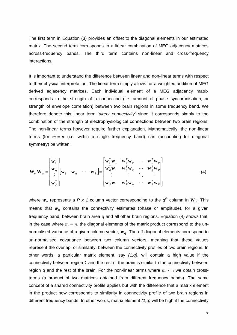
The non-linear terms however require further explanation. Mathematically, the non-linear
terms (for 𝑚 = 𝑛 (i.e. within a single frequency band) can (accounting for diagonal
symmetry) be written:
P
T
Pq
T
P
T
P
P
T
T
q
T
q
P
T
q
TT
Pq
T
P
T
q
T
mm
wwwwww
wwwwww
wwwwww
www
w
w
w
WW
1
1
1111
1
1
(4)
where 𝒘𝑞 represents a P x 1 column vector corresponding to the qth column in 𝐖𝑚. This
means that 𝒘𝑞 contains the connectivity estimates (phase or amplitude), for a given
frequency band, between brain area q and all other brain regions. Equation (4) shows that,
in the case where 𝑚 = 𝑛, the diagonal elements of the matrix product correspond to the un-
normalised variance of a given column vector, 𝒘𝑞. The off-diagonal elements correspond to
un-normalised covariance between two column vectors, meaning that these values
represent the overlap, or similarity, between the connectivity profiles of two brain regions. In
other words, a particular matrix element, say (1,q), will contain a high value if the
connectivity between region 1 and the rest of the brain is similar to the connectivity between
region q and the rest of the brain. For the non-linear terms where 𝑚 ≠ 𝑛 we obtain cross-
terms (a product of two matrices obtained from different frequency bands). The same
concept of a shared connectivity profile applies but with the difference that a matrix element
in the product now corresponds to similarity in connectivity profile of two brain regions in
different frequency bands. In other words, matrix element (1,q) will be high if the connectivity

8
between region 1 and the rest of the brain in frequency band A is similar to connectivity
between region q and the rest of the brain in frequency band B. Overall, the non-linear term
gives information about the potential contribution of shared electrophysiological connectivity
profiles (within and between frequency bands) to fMRI networks. We therefore term this non-
linear contribution ‘shared connectivity’.
Finally, note that as a further simplification for Equation (3), we consider an error matrix 𝐄
instead of the remainder R (= remainder of higher order terms) in order to compensate for
the unexplained portion of the approximation. This error matrix, E, contains an offset for all
non-diagonal elements, where 𝐄 = 𝑐(𝒖𝒖𝑇) and 𝒖 being the all-one vector and 𝑐 a scalar
coefficient (similar to the approach in (Meier et al., 2016)).
3) Methods
We used MEG and fMRI data obtained from two different datasets and research centres.
3.1) Subjects: dataset 1
Dataset 1 was acquired at the Sir Peter Mansfield Magnetic Resonance Centre, University of
Nottingham. Thirty-one healthy control subjects (age 27.4±6.4 (mean and standard
deviation), 40% female) with no history of neurological impairment were originally enrolled
and scanned as part of the University of Nottingham’s Multi-modal Imaging Study in
Psychosis. A number of subjects were excluded due to insufficient coverage in fMRI. This
resulted in a total of 15 participants (age 27.7±6.5 (mean and standard deviation), 60%
female) in the final analysis. The study was approved by the University of Nottingham
Medical School Ethics Committee, and all subjects gave written informed consent prior to
participation.
3.2) MEG data collection and pre-processing: dataset 1
MEG data were acquired using the third order synthetic gradiometer configuration of a 275
channel CTF MEG system (MISL, Coquitlam, Canada), at a sampling rate of 600Hz and
using a 150Hz low pass anti-aliasing filter. Magnetic fields were recorded during a task-free,
eyes-open condition for 10 minutes in a supine position. Subjects were asked to fixate on a
red cross throughout. Three coils were attached to the participant’s head as fiducial markers
at the nasion, left and right preauricular points. These coils were energised continuously
throughout acquisition to allow localisation of the head relative to the geometry of the MEG
sensor array. Before MEG acquisition, the surface of the participant’s head was digitised
using a 3D digitiser (Polhemus Inc., Vermont). Subsequent surface matching of the digitised
head shape to an equivalent head shape extracted from an anatomical magnetic resonance
9
(MR) image (see below for acquisition details) allowed coregistration of brain anatomy to
MEG sensor geometry.
Following collection, MEG data were inspected for artefacts generated by, for example, the
magnetomyogram, magnetooculogram and magnetocardiogram. Any trials deemed to
contain excessive interference generated via such sources were removed. In addition, trials
in which the participant was found to have moved more than 7 mm from their starting
position were also removed.
An atlas-based beamforming approach was adopted to project MEG sensor level data into
source-space (Hillebrand and Barnes, 2005; Hillebrand et al., 2012). The cortex was
parcellated into 78 individual regions according to the automated anatomical labelling (AAL)
atlas (Tzourio-Mazoyer et al., 2002). This was done by registering each subject’s anatomical
MR image to an MNI template and labelling all cortical voxels according to the 78 cortical
ROIs (Gong et al., 2009). Subsequently, an inverse registration to anatomical subject space
was performed. A beamformer (Robinson et al., 2012) was then employed to generate a
single signal representative of electrophysiological activity within each of these AAL regions.
To achieve this, for each region, first the centre of mass was derived. Voxels were then
defined on a regular 4 mm grid covering the entire region, and the beamformer estimated
timecourse of electrical activity was derived for each voxel. To generate a single timecourse
representing the whole region, denoted by �̂�𝑅(𝑡), individual voxel signals were weighted
according to their distance from the centre of mass such that,
�̂�𝑅(𝑡) = ∑ 𝑒𝑥𝑝(−𝑟𝑖
2
400⁄ )𝑖 �̂�𝑖(𝑡), (5)
where 𝑖 represents a count over all voxels within the AAL region, �̂�𝑖(𝑡) represents the
beamformer projected timecourse for voxel 𝑖, and 𝑟𝑖 denotes the distance (measured in
millimetres) to the centre of mass of the region. Note that the Gaussian weighting function
ensures that the regional timecourse �̂�𝑅(𝑡) was biased towards the centre of the region. The
full width at half maximum of the weighting was ~17mm.
To calculate the individual �̂�𝑖(𝑡), a scalar beamformer was used (Robinson et al., 2012).
Covariance was computed within a 1–150 Hz frequency window and a time window
spanning the whole experiment (excluding those trials removed due to interference)
(Brookes et al., 2008). Regularisation was applied to the data covariance matrix using the
10
Tikhonov method with a regularisation parameter equal to 5% of the maximum eigenvalue of
the unregularised covariance matrix. The forward model was based upon a dipole
approximation (Sarvas, 1987) and a multiple local sphere head model (Huang, 1999) fitted to
the MRI scalp surface as extracted from the co-registered MRI. Dipole orientation was
determined using a non-linear search for optimum signal to noise ratio (SNR, here computed
as the pseudo-Z value (Robinson et al., 2012)). Beamformer time-courses were sign-flipped
where necessary in order to account for the arbitrary polarity introduced by the beamformer
source orientation estimation.
This complete process resulted in 78 electrophysiological time-courses each representative
of a separate AAL region. This approach was applied to each subject individually.
3.3) fMRI data collection and pre-processing: dataset 1
MRI data were collected using a 7T-MRI system (Philips Achieva) with a volume transmit
and 32 channel receive head coil. The anatomical MR image (used for MEG source
reconstruction as well as fMRI processing) was acquired using an MPRAGE sequence (1
mm isotropic resolution, TE = 3 ms, TR = 7 ms, flip angle = 8˚). Bias fields were corrected
using SPM8 and brain extraction for the MPRAGE was achieved using the Brain Extraction
Tool (BET v2.1, FSL (FMRIB's Software Library, http://www.fmrib.ox.ac.uk/fsl)) (Smith et al.,
2004). Resting-state fMRI data were acquired using a gradient-echo echo planar imaging
sequence (TR = 2s, TE = 25ms, flip angle = 75 ˚, voxel dimensions = 2x2x2 mm3, 150
volume acquisitions). Participants were asked to keep their eyes open during the scan and
to fixate on a cross presented on a back projection screen and viewed through a mirror. Data
were motion corrected using SPM8 (Ashburner et al., 1999). Subject-specific masks of grey
matter, white matter, and cerebrospinal fluid (CSF) were obtained via automatic
segmentation of the MPRAGE data (FAST v4.1 FSL (Smith, 2002)).
The AAL atlas was used to parcellate the brain into the same 78 regions of interest (ROI) as
used for connectivity analysis in the MEG data (Gong et al., 2009). The fMRI data were
registered to the corresponding MPRAGE image, which was in turn registered to the MNI-
152 template brain (FLIRT v5.5, FSL, (Smith et al., 2004)). Inverse transformations were
calculated and used to register a grey matter mask and the AAL ROIs to the functional
space for each subject. These masks were then combined, to exclude white matter and CSF
voxels from further analysis. In order to maintain consistency between the fMRI and MEG
pipeline, a weighted average fMRI signal was computed to obtain a single signal for every
ROI. This was done using the function in Equation (5). See SI Figure S1 for comparison with
unweighted average over voxels in a ROI, which showed no measurable difference in
11
connectivity between the two approaches. We then regressed out average cerebrospinal
fluid signal, average white matter signal, motion and 2nd order polynomials (i.e. low
frequency trends) from each regional BOLD timecourse using a general linear model in order
to remove non-neuronal signals. Note that the effect of ordering (averaging and then
regressing out nuisance variables or vice versa) was assessed; the results can be found in
SI Figure S2. The effect of average translational motion during the fMRI scan on the average
functional connectivity was also assessed (Spearman correlation R=0.01, p=0.9).
3.4) Dataset 2
Dataset 2 was acquired at the VU Medical Centre (VUmc), VU University, Amsterdam.
Twenty-one healthy control subjects with no history of neurological impairment (age
42.5±10.3 (mean and standard deviation), 65.1% female) were scanned as part of an
ongoing multiple sclerosis study (Tewarie et al., 2015). The study was approved by the
Ethics Review Board of the VUmc and all subjects gave written informed consent prior to
participation. The data collection and pre-processing steps of the second dataset are
described in a previous paper (Tewarie et al., 2015) and in the supplementary material. This
dataset was used here for validation of the Taylor coefficients obtained from dataset 1. The
main differences to dataset 1 with respect to MEG were 1) The instrument manufacturer (a
306 channel Elekta-NeuroMag system was employed) and 2) A peak voxel approach was
employed, meaning that the voxel with maximum power in each AAL region was used as
representative time-series for each ROI (as distinct from the Gaussian weighting). For fMRI,
there were more pipeline differences between the two datasets: 1) A 3T MRI system, rather
than a 7T system, was used. 2) We employed non-linear registration rather than linear
registration. 3) Spatial smoothing was used, and high-pass filtering rather than polynomial
regression was employed. 4) We omitted regression of average cerebrospinal fluid signal,
average white matter signal and motion parameters. 5) We computed an unweighted
average over voxels across each AAL region rather than a weighted average to derive a
representative time signal for a ROI.
3.5) Construction of fMRI/MEG networks
For each subject’s fMRI data, we computed pairwise Pearson correlation coefficients
between all possible 78 fMRI AAL signal pairs in order to obtain a symmetric 78x78 fMRI
network, described by its weighted adjacency matrix. Negative correlation values were left
intact. For MEG, we evaluated two different intrinsic modes of functional connectivity; a
phase based and an amplitude based measure. Specifically, the phase lag index (PLI) (Stam
et al., 2007) and the average envelope correlation (AEC) (Brookes et al., 2011a) were
computed between all possible pairs of beamformer projected regional time-series to obtain
12
symmetric 78x78 MEG networks for each subject. Note that this was done independently
within 5 separate frequency bands (delta (1-4Hz), theta (4-8Hz), alpha (8-13Hz), beta (13-
30Hz), gamma (30-48)). The PLI is a metric that captures the asymmetry of the phase
difference distribution of two time-series (see SI for further details), whereas the AEC
computes the correlation between the envelope of two time-series (see SI for further details;
(Brookes et al., 2012b; Hipp et al., 2012)). Note that PLI is inherently robust to source
leakage artifact. An orthogonalisation procedure (as in (Brookes et al., 2012b)) was
employed for AEC to ensure that adjacency matrices were not dominated by the leakage
artefact. Overall applying these metrics to the data resulted in 11 adjacency matrices per
subject; 5 MEG based PLI matrices; 5 MEG based AEC matrices, and a single fMRI matrix.
These 11 separate adjacency matrices were averaged across subjects and taken forward for
further analysis. The rationale for the latter is that averaging across subjects will lead to a
reduction of noise in the adjacency matrices.
3.6) Taylor series combination of weighted adjacency matrices
Figure 1: Flow chart of the analysis pipeline. For both MEG and fMRI we averaged the connectivity
matrices across subjects to obtain one group averaged connectivity matrix. For MEG, this was done
for each frequency band and connectivity metric separately. The MEG matrices displayed here
correspond to the AEC measurement obtained from the first dataset. We then followed a step-by-step
approach to approximate group averaged fMRI networks based upon MEG matrices (level 1). We
included: individual frequency bands for each metric separately (model a); multiple frequency bands
in a linear combination for each metric separately (model b), multiple frequency bands in a linear plus
non-linear combination for each metric separately, (cross-terms excluded) (model c); Equivalent to
model c but now with the cross-terms included (model d), multiple frequency bands and metrics in a
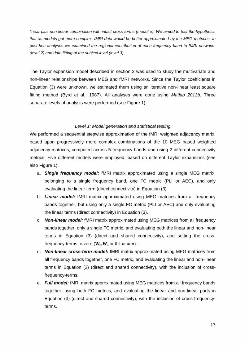
13
linear plus non-linear combination with intact cross-terms (model e). We aimed to test the hypothesis
that as models got more complex, fMRI data would be better approximated by the MEG matrices. In
post-hoc analyses we examined the regional contribution of each frequency band to fMRI networks
(level 2) and data fitting at the subject level (level 3).
The Taylor expansion model described in section 2 was used to study the multivariate and
non-linear relationships between MEG and fMRI networks. Since the Taylor coefficients in
Equation (3) were unknown, we estimated them using an iterative non-linear least square
fitting method (Byrd et al., 1987). All analyses were done using Matlab 2013b. Three
separate levels of analysis were performed (see Figure 1).
Level 1: Model generation and statistical testing
We performed a sequential stepwise approximation of the fMRI weighted adjacency matrix,
based upon progressively more complex combinations of the 10 MEG based weighted
adjacency matrices, computed across 5 frequency bands and using 2 different connectivity
metrics. Five different models were employed, based on different Taylor expansions (see
also Figure 1):
a. Single frequency model: fMRI matrix approximated using a single MEG matrix,
belonging to a single frequency band, one FC metric (PLI or AEC), and only
evaluating the linear term (direct connectivity) in Equation (3).
b. Linear model: fMRI matrix approximated using MEG matrices from all frequency
bands together, but using only a single FC metric (PLI or AEC) and only evaluating
the linear terms (direct connectivity) in Equation (3).
c. Non-linear model: fMRI matrix approximated using MEG matrices from all frequency
bands together, only a single FC metric, and evaluating both the linear and non-linear
terms in Equation (3) (direct and shared connectivity), and setting the cross-
frequency-terms to zero (𝐖𝑚𝐖𝑛 = 0 if 𝑚 ≠ 𝑛).
d. Non-linear cross-term model: fMRI matrix approximated using MEG matrices from
all frequency bands together, one FC metric, and evaluating the linear and non-linear
terms in Equation (3) (direct and shared connectivity), with the inclusion of cross-
frequency-terms.
e. Full model: fMRI matrix approximated using MEG matrices from all frequency bands
together, using both FC metrics, and evaluating the linear and non-linear parts in
Equation (3) (direct and shared connectivity), with the inclusion of cross-frequency-
terms.
14
For models a-e above, the success of combined MEG matrices in predicting the fMRI matrix
was evaluated using a goodness-of-fit measure (R2).
We aimed to test two separate hypotheses:
1) MEG derived matrices, combined using all of the Taylor based models listed above,
predict a significant amount of variance in the fMRI matrix.
2) Moving to progressively more complex models (i.e. adding extra terms) significantly
improves prediction of the fMRI matrix.
In order to test these two hypotheses statistically, we employed a permutation approach in
which pseudo-matrices were generated. To obtain these pseudo-matrices we first performed
an eigenvalue decomposition of the real MEG derived matrices. Each eigenvector was then
randomised using a phase based technique (O'Neill et al., 2015; Prichard and Theiler, 1994)
(see appendix for further details). Reconstruction of the matrix post-randomisation yielded a
pseudo-matrix, similar in mathematical structure to the genuine adjacency matrices, but not
reflecting genuine MEG derived functional connectivity. Using these pseudo-matrices we
performed the following tests:
Test 1: To test hypothesis 1 we employed 1000 iterations of a permutation test (Nichols
and Holmes, 2002). On each iteration, a new set of 10 MEG pseudo matrices were
generated (each based upon the 10 genuine MEG derived matrices). They were
combined using the Taylor expansion for all models (a-e above), and the extent to which
they could predict the fMRI matrix was measured via the R2 value. This generated an
empirical null distribution based upon 1000 R2 values denoting the extent to which fMRI
connectivity could be predicted by pseudo-matrices. Comparison of this null distribution
with the genuine R2 value (from the real MEG matrices) then allowed calculation of a p-
value representing the probability that variance explained in fMRI by models a-e above
could have occurred by chance. Results were considered significant at a p-value of up to
0.05, corrected for multiple comparisons (Bonferroni) for the 5 separate tests over all five
models.
Testing hypothesis 2 is non-trivial, since it is always the case that adding more terms to a
model would likely improve variance explained. Two separate tests were run:
Test 2a: We first derived R2 values from each of the models (a-e) using real MEG
derived matrices. A gradient was measured representing the rate of improvement of R2
with increasing model complexity. Across 1000 iterations, we then constructed a null
distribution where this same gradient was measured, but using ‘sham’ R2 values derived
from pseudo-matrices. Note that for the ‘sham’ R2 values we would also expect an
improvement in variance explained with increasing model complexity, and therefore a
positive gradient (since adding additional terms usually leads to more variance
15
explained). However rejection of the null hypothesis would suggest that the rate of
improvement observed in real data did not occur by chance. Comparison of this
empirical null distribution with the genuine gradient allowed calculation of a p-value.
Results were considered significant at p<0.05.
Test 2b: For each of the 3 increments in model complexity (1: moving from a single
frequency to a linear model; 2: moving from a linear to a non-linear model; 3: moving
from a non-linear to a non-linear plus cross term model) we tested whether each step
generated a significant increase in R2. To do this, we first measured the difference in R2
between successive models using the MEG derived matrices. Again over 1000
iterations, we then measured the same difference using pseudo-matrices, thus
constructing a null distribution. Comparison of the null distribution with the genuine R2
difference allowed calculation of a p-value. Results were considered significant at a p-
value of less than 0.05, corrected for multiple comparisons (Bonferroni) for the 3
separate tests.
These three separate tests (1a, 2a, 2b) allowed direct testing of our two primary hypotheses.
Finally, in order to further validate our Taylor models, we measured correlation in the Taylor
parameters (i.e. am, bmn from Equation (3)) derived via application of the models to dataset 1
and dataset 2. Here, we reasoned that if the models used were genuinely reflective of an
MEG to fMRI network mapping, then the parameters would be significantly correlated across
these two completely independent datasets.
Level 2: The contribution of each frequency band
Given the prior knowledge that MEG networks show frequency specific structure, we
expected to see the same patterns in the prediction of fMRI networks. Therefore, we
examined the contribution of each MEG frequency band separately to the fMRI network by
inspecting the regional connections explained by each band. Results were based on the
approximation from our single frequency model (model a), and the percentage of
connections shown was based on the obtained R2 (e.g. for R2 = 0.1, top 10% of connections
displayed). These analyses were only done for model a since the end results of estimations
from the other models were obtained by a weighted sum of all frequencies.
Level 3: Individual subject analysis
The most accurate model from level 1a-d was used within each individual subject in order to
address how well MEG weighted adjacency matrices computed within a single individual can
predict their fMRI counterpart. PLI and AEC obtained results were compared using a Mann-
Whitney U test. In order to assess this statistically, we performed permutation analysis
(Nichols and Holmes, 2002). We reasoned that if the two modalities contained subject
16
specific information, then the MEG derived networks from subject A would be a better
predictor of the fMRI network from subject A, compared to, for example, the MEG networks
from subject B. To this end, we swapped MEG networks randomly across subjects to get
unmatched pairs of MEG and fMRI networks, from which a null-distribution of R2 values was
generated (N = 1000 permutations). The genuine R2 was compared against this null
distribution using a significance level of 5%.
4) Results
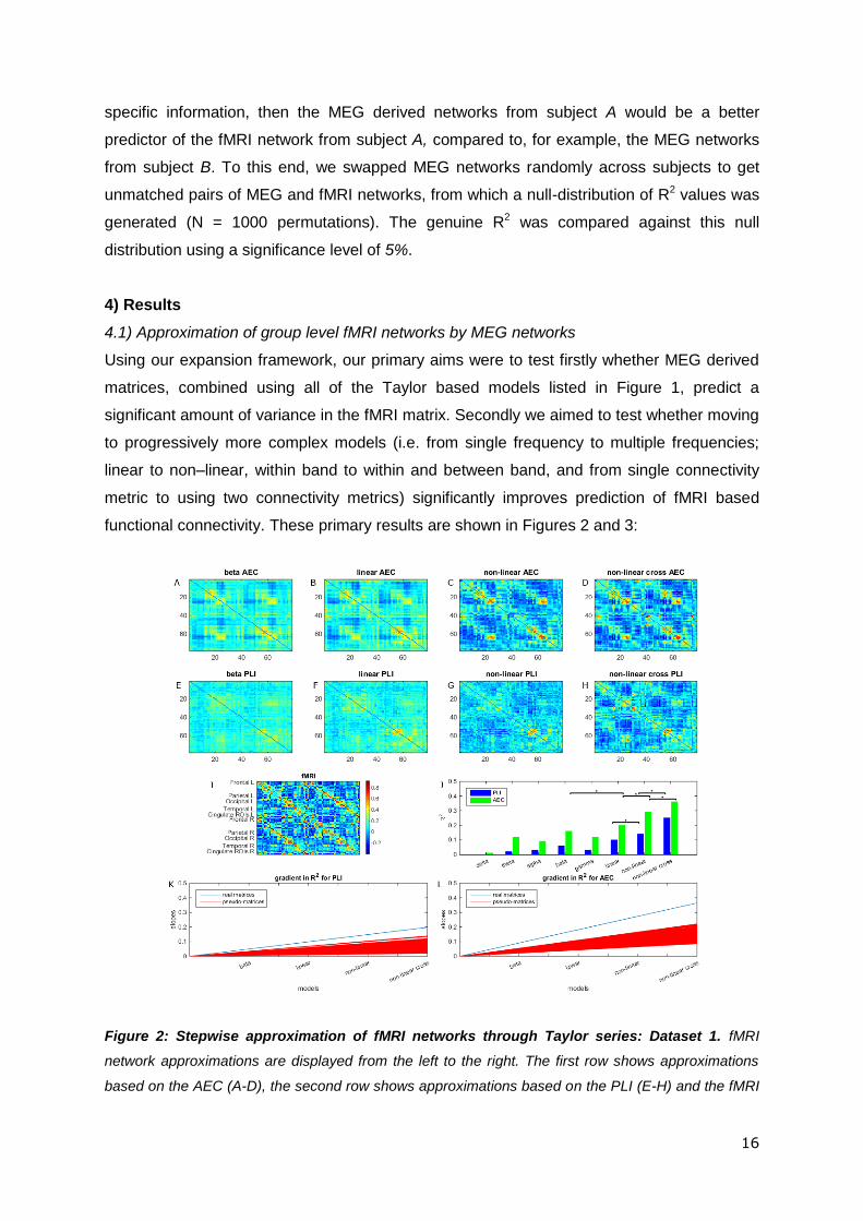
4.1) Approximation of group level fMRI networks by MEG networks
Using our expansion framework, our primary aims were to test firstly whether MEG derived
matrices, combined using all of the Taylor based models listed in Figure 1, predict a
significant amount of variance in the fMRI matrix. Secondly we aimed to test whether moving
to progressively more complex models (i.e. from single frequency to multiple frequencies;
linear to non–linear, within band to within and between band, and from single connectivity
metric to using two connectivity metrics) significantly improves prediction of fMRI based
functional connectivity. These primary results are shown in Figures 2 and 3:
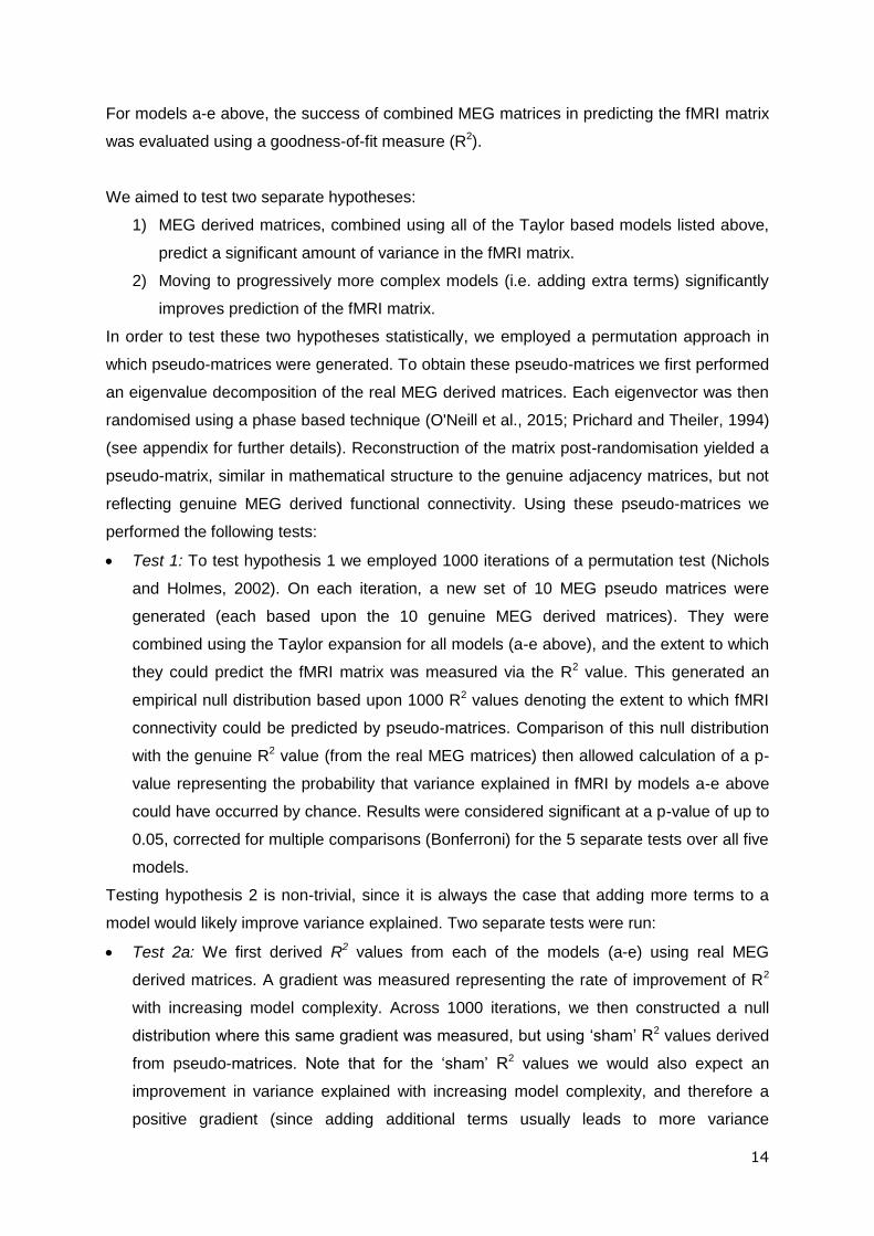
Figure 2: Stepwise approximation of fMRI networks through Taylor series: Dataset 1. fMRI
network approximations are displayed from the left to the right. The first row shows approximations
based on the AEC (A-D), the second row shows approximations based on the PLI (E-H) and the fMRI
17
network is displayed in the third row (I) together with a colour bar that is the same for all the matrices
shown. The ROIs are ordered according to (Gong et al., 2009). Results are shown, from left to right,
for the single frequency model (A, E), the linear model (B, F), the non-linear model (C, G), and the
non-linear cross-term model (D, H). In the third row, the bar chart shows the R2 values using either
combinations of AEC matrices (green) or PLI matrices (blue) (J). A clear improvement in explained
variance can be seen as more terms are included in the model, i.e. when moving from the specific
frequency band predictions, to the approximations that include multiple frequency bands, nonlinearity
and cross-terms. This is the case for both the AEC and PLI. These improvements are significant
beyond chance, as can be seen by the results of the permutation tests; here * denotes statistical
significance (p<0.015; Bonferroni corrected for three tests; test 2b). Note that only the best single
frequency model (beta band) was included for the analysis). This stepwise improvement is also
apparent from the estimated fMRI matrices (first and second row), with the best approximations in the
right hand column (E, H). This can be seen from the increasing number of strong connections near
the diagonal and the two off-diagonals. A gradient for the genuine rate of improvement of R2 (blue)
with increasing model complexity and rate of improvement from 1000 permutations (red) is depicted in
(K) for PLI (test 2a; p<0.001) and in (L) for AEC (test 2a; p<0.001).
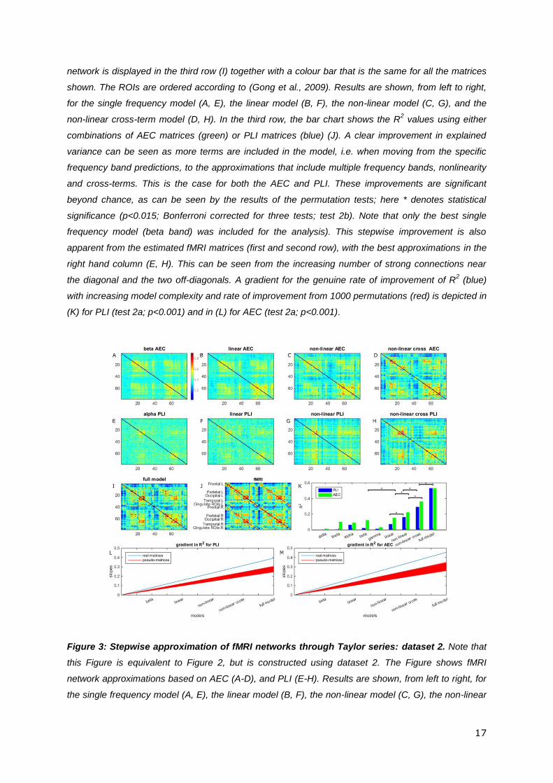
Figure 3: Stepwise approximation of fMRI networks through Taylor series: dataset 2. Note that
this Figure is equivalent to Figure 2, but is constructed using dataset 2. The Figure shows fMRI
network approximations based on AEC (A-D), and PLI (E-H). Results are shown, from left to right, for
the single frequency model (A, E), the linear model (B, F), the non-linear model (C, G), the non-linear
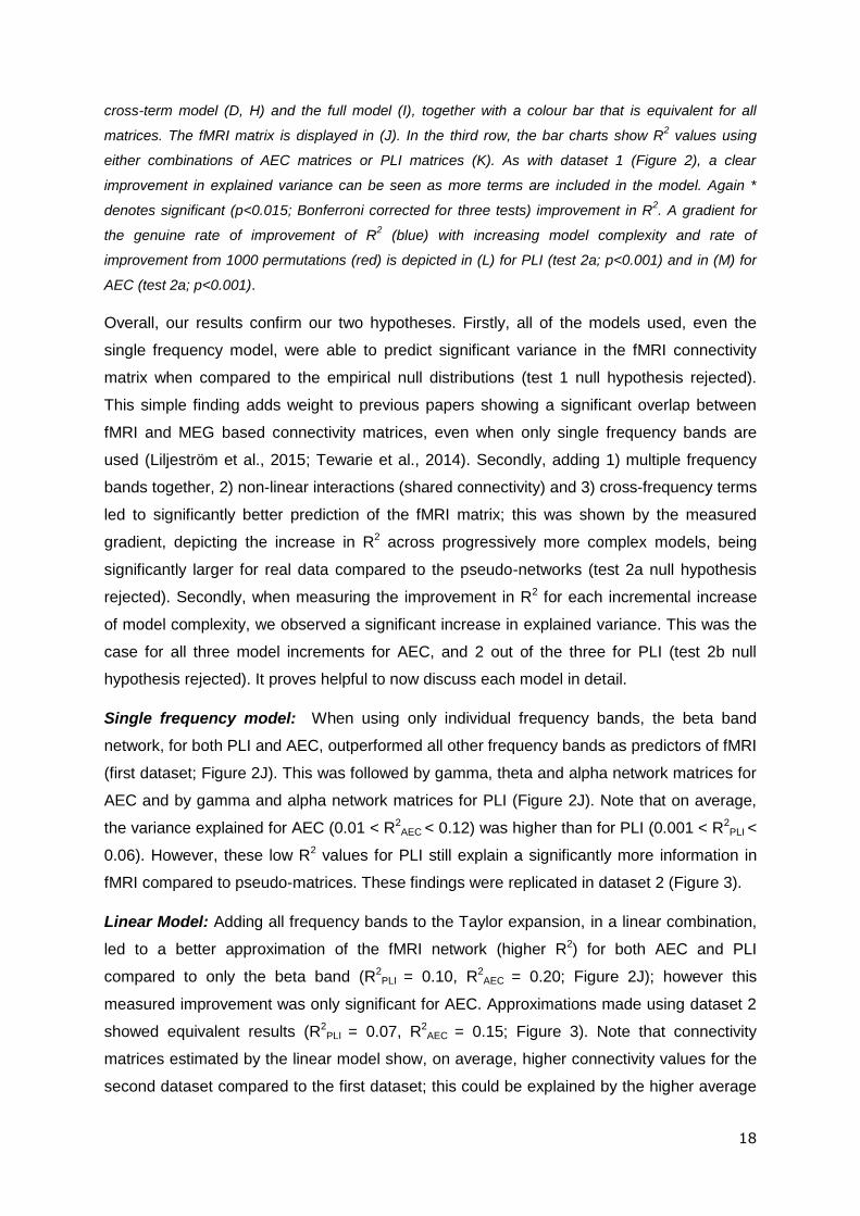
18
cross-term model (D, H) and the full model (I), together with a colour bar that is equivalent for all
matrices. The fMRI matrix is displayed in (J). In the third row, the bar charts show R2 values using
either combinations of AEC matrices or PLI matrices (K). As with dataset 1 (Figure 2), a clear
improvement in explained variance can be seen as more terms are included in the model. Again *
denotes significant (p<0.015; Bonferroni corrected for three tests) improvement in R2. A gradient for
the genuine rate of improvement of R2 (blue) with increasing model complexity and rate of
improvement from 1000 permutations (red) is depicted in (L) for PLI (test 2a; p<0.001) and in (M) for
AEC (test 2a; p<0.001).
Overall, our results confirm our two hypotheses. Firstly, all of the models used, even the
single frequency model, were able to predict significant variance in the fMRI connectivity
matrix when compared to the empirical null distributions (test 1 null hypothesis rejected).
This simple finding adds weight to previous papers showing a significant overlap between
fMRI and MEG based connectivity matrices, even when only single frequency bands are
used (Liljeström et al., 2015; Tewarie et al., 2014). Secondly, adding 1) multiple frequency
bands together, 2) non-linear interactions (shared connectivity) and 3) cross-frequency terms
led to significantly better prediction of the fMRI matrix; this was shown by the measured
gradient, depicting the increase in R2 across progressively more complex models, being
significantly larger for real data compared to the pseudo-networks (test 2a null hypothesis
rejected). Secondly, when measuring the improvement in R2 for each incremental increase
of model complexity, we observed a significant increase in explained variance. This was the
case for all three model increments for AEC, and 2 out of the three for PLI (test 2b null
hypothesis rejected). It proves helpful to now discuss each model in detail.
Single frequency model: When using only individual frequency bands, the beta band
network, for both PLI and AEC, outperformed all other frequency bands as predictors of fMRI
(first dataset; Figure 2J). This was followed by gamma, theta and alpha network matrices for
AEC and by gamma and alpha network matrices for PLI (Figure 2J). Note that on average,
the variance explained for AEC (0.01 < R2AEC
< 0.12) was higher than for PLI (0.001 < R2PLI
<
0.06). However, these low R2 values for PLI still explain a significantly more information in
fMRI compared to pseudo-matrices. These findings were replicated in dataset 2 (Figure 3).
Linear Model: Adding all frequency bands to the Taylor expansion, in a linear combination,
led to a better approximation of the fMRI network (higher R2) for both AEC and PLI
compared to only the beta band (R2PLI
= 0.10, R2AEC
= 0.20; Figure 2J); however this
measured improvement was only significant for AEC. Approximations made using dataset 2
showed equivalent results (R2PLI
= 0.07, R2AEC
= 0.15; Figure 3). Note that connectivity
matrices estimated by the linear model show, on average, higher connectivity values for the
second dataset compared to the first dataset; this could be explained by the higher average
19
connectivity in the fMRI matrix and/or the shorter window length used for the second dataset,
which can bias the AEC/PLI towards higher values. The confidence intervals of the
estimated Taylor coefficients for datasets 1 and 2 overlapped (Figure S3 and S4) and the
coefficients themselves showed significant correlation for both functional connectivity metrics
(rPLI(6) = 0.86 p = 0.03; rAEC(6) = 0.93 p = 0.006), indicating robustness of the mapping
across two independent datasets.
Non-linear model: We evaluated the Taylor coefficients corresponding to both linear and
non-linear terms in order to investigate potential contribution of shared electrophysiogical
connectivity to fMRI. To exclude cross-frequency interactions, we removed the cross-terms
in Equation (3) (i.e. all 𝑚 ≠ 𝑛). A significant increase in explained variance was observed for
both AEC and PLI compared to including linear terms only (R2PLI
= 0.14, R2AEC
= 0.29; Figure
2C, G). The second dataset showed equivalent results (R2PLI
= 0.16, R2AEC
= 0.22). There
was significant correlation between the Taylor coefficients for datasets 1 and 2 for AEC
(rAEC(11) = 0.76 p = 0.007) indicating robustness of the mapping. However this was not the
case for PLI, rPLI(11) = 0.49 and p = 0.14)
Non-linear model with cross-terms: We repeated the non-linear model, but with cross-
terms retained, which allows examination of the contribution of cross-frequency shared
connectivity to fMRI. Adding cross-frequency terms led to significantly better fMRI network
approximations for both dataset 1 (R2PLI
= 0.25, R2AEC
= 0.36; Figure 2J) and dataset 2 (R2PLI
= 0.29, R2AEC
= 0.36; Figure 3K), for both PLI and AEC, compared to the approximation when
cross-terms were ignored. The Taylor coefficients and their confidence intervals for the
approximation based on the AEC again largely overlapped and correlated significantly
(rAEC(30) = 0.48, p = 0.007; Figure S5). For PLI this was not the case (rPLI(30) = 0.26, p =
0.15; Figure S6) since the Taylor coefficients of the first dataset displayed large confidence
intervals. For all analysis levels up to the linear cross-term model we analysed whether we
could observe standard resting state networks (RSNs ) in the whole brain approximations as
credibility check for our results (e.g. default mode-, sensorimotor-, salience-, fronto-parietal-,
executive-, and the visual-network). The clearest RSN patterns could be observed for AEC
in the approximations based on the non-linear cross-term model (see Figure S7).
Full Model: Finally, we assessed whether adding the two modes of connectivity (AEC and
PLI) would improve our approximation. Since estimated parameters for PLI were associated
with large confidence intervals in the non-linear cross-term model for dataset 1, we restricted
this analysis to dataset 2. Note that adding PLI and AEC network matrices together into
Equation (3) resulted in ten different matrices, and therefore 110 Taylor coefficients to
estimate. Given the number of matrix elements (𝑁2−𝑁
2= 3003), the number of coefficients is
20
still relatively small so that overfitting based on numerous parameters is not an issue. After
evaluation of Equation (3) we obtained an R2 = 0.53 (Figures 3I and 3K). Although the
current fit involved estimation of 110 coefficients, the confidence intervals were still small
and did not become unstable, as was the case for the analysis with PLI (non-linear cross-
term model) for dataset 1 (Figure S8).
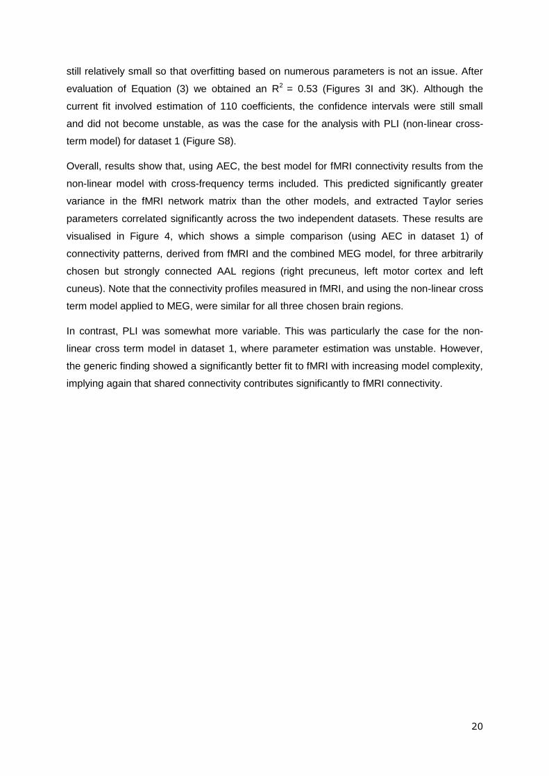
Overall, results show that, using AEC, the best model for fMRI connectivity results from the
non-linear model with cross-frequency terms included. This predicted significantly greater
variance in the fMRI network matrix than the other models, and extracted Taylor series
parameters correlated significantly across the two independent datasets. These results are
visualised in Figure 4, which shows a simple comparison (using AEC in dataset 1) of
connectivity patterns, derived from fMRI and the combined MEG model, for three arbitrarily
chosen but strongly connected AAL regions (right precuneus, left motor cortex and left
cuneus). Note that the connectivity profiles measured in fMRI, and using the non-linear cross
term model applied to MEG, were similar for all three chosen brain regions.
In contrast, PLI was somewhat more variable. This was particularly the case for the non-
linear cross term model in dataset 1, where parameter estimation was unstable. However,
the generic finding showed a significantly better fit to fMRI with increasing model complexity,
implying again that shared connectivity contributes significantly to fMRI connectivity.
21
Figure 4: Estimated fMRI connections for individual regions. Arbitrary thresholded fMRI
connections for three regions (right precuneus, left motor cortex and left cuneus) are shown in (A) on
a template mesh. Panel (B) shows connectivity from the same seed regions based on the non-linear
cross-term model, obtained with AEC.
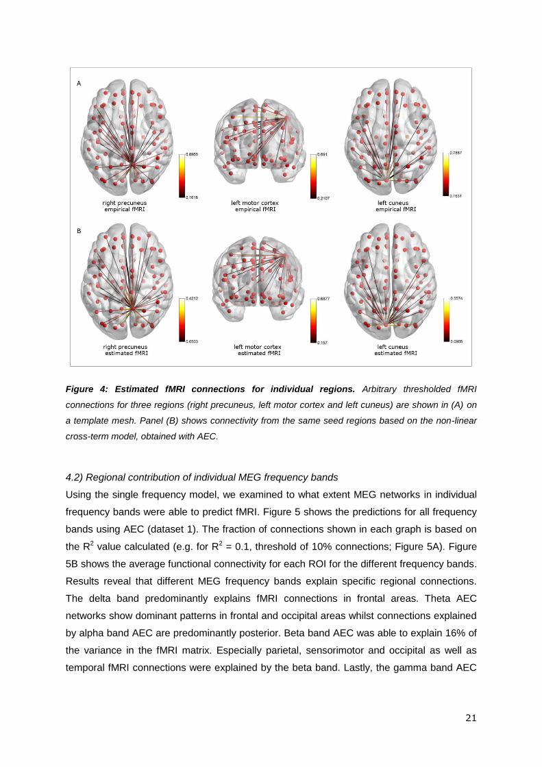
4.2) Regional contribution of individual MEG frequency bands
Using the single frequency model, we examined to what extent MEG networks in individual
frequency bands were able to predict fMRI. Figure 5 shows the predictions for all frequency
bands using AEC (dataset 1). The fraction of connections shown in each graph is based on
the R2 value calculated (e.g. for R2 = 0.1, threshold of 10% connections; Figure 5A). Figure
5B shows the average functional connectivity for each ROI for the different frequency bands.
Results reveal that different MEG frequency bands explain specific regional connections.
The delta band predominantly explains fMRI connections in frontal areas. Theta AEC
networks show dominant patterns in frontal and occipital areas whilst connections explained
by alpha band AEC are predominantly posterior. Beta band AEC was able to explain 16% of
the variance in the fMRI matrix. Especially parietal, sensorimotor and occipital as well as
temporal fMRI connections were explained by the beta band. Lastly, the gamma band AEC
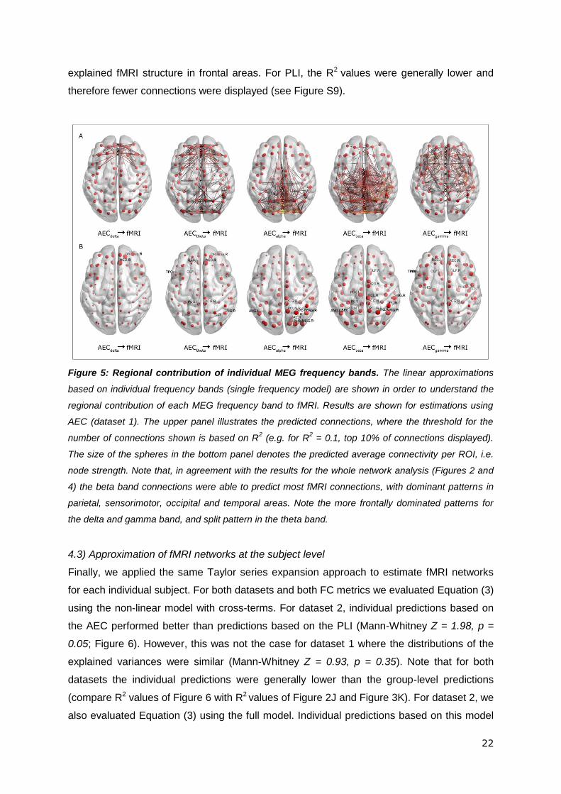
22
explained fMRI structure in frontal areas. For PLI, the R2 values were generally lower and
therefore fewer connections were displayed (see Figure S9).
Figure 5: Regional contribution of individual MEG frequency bands. The linear approximations
based on individual frequency bands (single frequency model) are shown in order to understand the
regional contribution of each MEG frequency band to fMRI. Results are shown for estimations using
AEC (dataset 1). The upper panel illustrates the predicted connections, where the threshold for the
number of connections shown is based on R2 (e.g. for R
2 = 0.1, top 10% of connections displayed).
The size of the spheres in the bottom panel denotes the predicted average connectivity per ROI, i.e.
node strength. Note that, in agreement with the results for the whole network analysis (Figures 2 and
4) the beta band connections were able to predict most fMRI connections, with dominant patterns in
parietal, sensorimotor, occipital and temporal areas. Note the more frontally dominated patterns for
the delta and gamma band, and split pattern in the theta band.
4.3) Approximation of fMRI networks at the subject level
Finally, we applied the same Taylor series expansion approach to estimate fMRI networks
for each individual subject. For both datasets and both FC metrics we evaluated Equation (3)
using the non-linear model with cross-terms. For dataset 2, individual predictions based on
the AEC performed better than predictions based on the PLI (Mann-Whitney Z = 1.98, p =
0.05; Figure 6). However, this was not the case for dataset 1 where the distributions of the
explained variances were similar (Mann-Whitney Z = 0.93, p = 0.35). Note that for both
datasets the individual predictions were generally lower than the group-level predictions
(compare R2 values of Figure 6 with R2 values of Figure 2J and Figure 3K). For dataset 2, we
also evaluated Equation (3) using the full model. Individual predictions based on this model
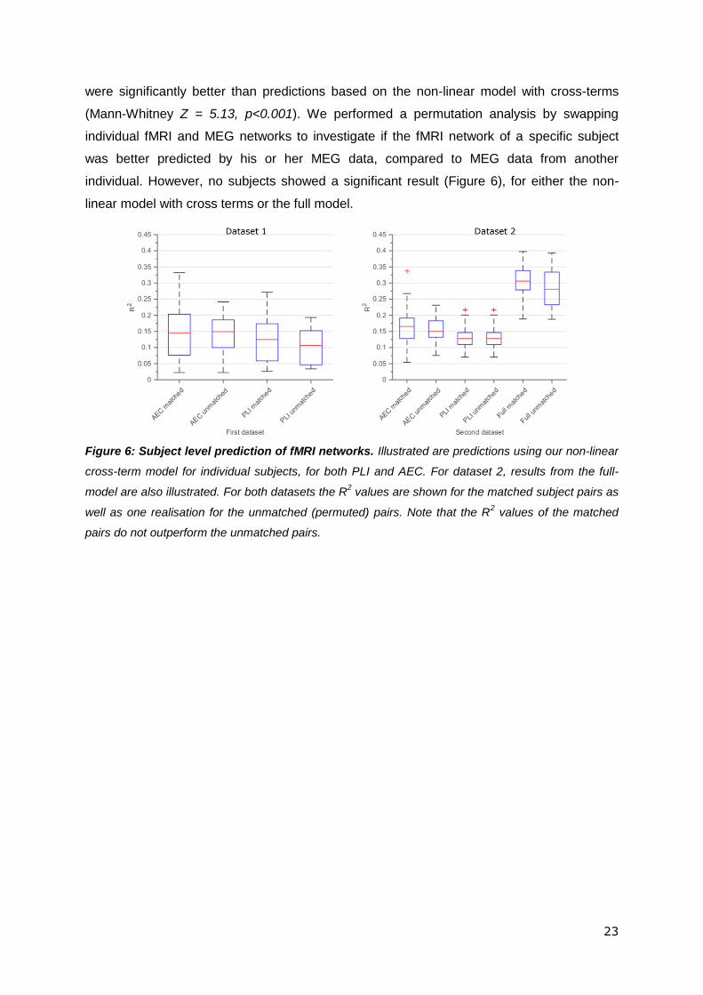
23
were significantly better than predictions based on the non-linear model with cross-terms
(Mann-Whitney Z = 5.13, p<0.001). We performed a permutation analysis by swapping
individual fMRI and MEG networks to investigate if the fMRI network of a specific subject
was better predicted by his or her MEG data, compared to MEG data from another
individual. However, no subjects showed a significant result (Figure 6), for either the non-
linear model with cross terms or the full model.
Figure 6: Subject level prediction of fMRI networks. Illustrated are predictions using our non-linear
cross-term model for individual subjects, for both PLI and AEC. For dataset 2, results from the full-
model are also illustrated. For both datasets the R2 values are shown for the matched subject pairs as
well as one realisation for the unmatched (permuted) pairs. Note that the R2 values of the matched
pairs do not outperform the unmatched pairs.
24
5) Discussion
In this study we investigated the relationship between electrophysiological and
haemodynamic networks, using a unique mathematical framework based upon the
assumption that the relationship between MEG and fMRI can be considered as a
mathematical function that can be analysed using a multivariate Taylor series. This
framework allowed us to integrate MEG data from multiple frequency bands and connectivity
metrics, together with linear and non-linear interaction terms, to predict fMRI networks. Our
main finding is that, although single frequency band MEG derived networks explain
significant variance in the fMRI network matrix, the accuracy of predicted fMRI networks
drastically improved when we considered the multivariate, linear, non-linear and cross-
frequency combinations of MEG features.
Using a single frequency model, we were able to find spectral specificity in regional fMRI
connections. Overall, the beta frequency band was the best predictor of fMRI connections in
both AEC and PLI and this finding is in agreement with earlier studies that have generally
shown significant agreement between fMRI and MEG beta band derived resting state
networks (see (Hall et al., 2014) for a review). Here (Figure 5) we have shown that parietal,
sensorimotor, occipital and temporal fMRI connections were well explained by MEG beta
band networks. Interestingly however, frontal connections in fMRI were better explained by
the theta and gamma frequency bands, whereas the alpha band predominantly explained
occipital/parietal connectivity. Anterior-posterior connections were observed in both the
alpha and theta bands, which has also been shown in a previous directed connectivity study
(Hillebrand et al., 2015). The presence of frequency specific regional connections, and their
regional distribution, is in line with recent work on the relationship between MEG and fMRI
(Hipp and Siegel, 2015). Overall this implies that fMRI must be seen as an integral of
multiple electrophysiological networks that occur on a variety of temporal scales.
The spatial inhomogeneity in MEG connectivity across-frequency bands suggests that
integrating multiple frequencies into a single description, using a linear model, would
improve prediction of fMRI. We used our Taylor model to show that, for envelope based
networks, this was indeed the case with a significant improvement in R2 when using a linear
combination of frequency bands. Therefore, fMRI networks may well result from a
combination of frequency bands, where each separate band adds regionally specific
information (Mantini et al., 2007). In regions where two frequency bands show similarity, for
example in occipital areas where alpha and beta connections overlap, an fMRI connection
could be considered as a weighted sum across those bands. Whilst PLI showed
25
improvement in R2 between the single frequency and the linear model, this failed to reach
significance. It is important to note that the estimated Taylor coefficients for the linear model
suggested that all frequency bands were represented, with no disproportionally high
coefficients, and no bands that could be neglected. This said, delta band connectivity
consistently contributed the least to fMRI. Importantly, the linear contribution of separate
frequency bands to the fMRI predictions was consistent between both datasets; this was
shown by both overlap in estimated Taylor coefficients as well as a significant correlation
between them. This result is extremely important as it underlines the robustness of our
mapping approach.
Adding non-linearity to the Taylor expansion significantly improved our approximation of
fMRI networks; this was true for both AEC and PLI. Importantly, this was not simply the
result of adding increased model complexity, since this was accounted for in our statistical
testing. The non-linear models included quadratic terms for each individual frequency band
as well as cross-terms between frequency bands. Here the independent addition of both
generated a significant improvement in fMRI prediction. The non-linear terms effectively
measure covariance between the neuronal connectivity profiles of separate regions (see
Equation (4)). The physical interpretation of the non-linear terms helps explain why their
addition improves the prediction of fMRI matrices: If two regions are electrophysiologically
interacting with similar areas, i.e. share the same connectivity profile, then it is likely that
their energy demands (i.e. their BOLD signals) are influenced in a similar fashion by those
shared connections. This likely increases the temporal correlation between BOLD signals,
and hence increases haemodynamic functional connectivity. The effect of shared
connectivity profiles on BOLD correlations also extends to cross-frequency terms. The
reader should note that the cross-frequency terms in our model do not contain direct cross-
frequency coupling between regions (e.g. a direct link between, for example, alpha in region
1 and gamma in region 2, as is often derived in, e.g. phase-amplitude coupling (Aru et al.,
2015; Jensen and Colgin, 2007)). Rather, our cross-frequency terms correspond to shared
connectivity patterns between independent networks existing within different frequency
bands. Their interpretation is therefore similar to that for non-linear terms within frequency
bands. Overall, our result suggests that BOLD connectivity results from not only direct
neuronal connectivity (i.e. an electrophysiological connection between the two regions in
question) but also shared connectivity profiles both within and between frequency bands.
This important result should be considered in future multi-modal connectivity studies.
In our Taylor series approximations, we also evaluated the role of the different intrinsic
coupling modes (phase (PLI) and amplitude (AEC)). Separate analysis for the AEC and PLI
26
revealed that AEC derived networks were better predictors for fMRI than PLI derived
networks. This was the case for all models (single frequency, linear and non-linear (with and
without cross-terms), and for both datasets). This result is also in agreement with previous
work on phase versus amplitude based interhemispheric sensorimotor network coupling
(Brookes et al., 2011a). The reason for this might be twofold: Firstly, the AEC networks
show more spatial structure than the PLI networks, which have a more random appearance
(see Figures S10 and S11 for spatial structure of the MEG matrices). This higher noise
would likely lead to less explained variance for the PLI estimations. The more random
appearance of PLI could result from multiple effects. This could be related to the fact that
larger phase differences are needed for AEC than for PLI in order to be able to detect a
functional connection (Hipp et al., 2012), and therefore the AEC matrices might contain more
false negative values and PLI more false-positive values, leading to a more structured
network for AEC. The more random appearance of PLI compared to AEC is certainly a
consistent feature of all data in this study, and future investigation using 1) voxel rather than
regional time-courses and 2) non-stationary rather than stationary connectivity might shed
light on this observation. A second possible reason for the close relationship between AEC
and fMRI may be that AEC is based on the envelopes of a time-series, which evolves on a
slower time-scale than the phase information; it may therefore be more closely related to the
BOLD signal. This said, combining AEC and PLI does add information in terms of explaining
fMRI networks: Using our full model, we combined AEC and PLI in a multivariate non-linear
approximation and this led to a higher explained variance than an approximation based on
AEC alone (or PLI alone), indicating that fMRI networks also reflect the sum of amplitude
and phase interactions. However, note that a multivariate non-linear approximation with two
connectivity measures only gave a maximum R2 of 0.5.It is possible that addition of higher
order terms would improve the approximation, or that the unexplained variance in fMRI is the
result of non-neuronal signal (Birn et al., 2008), noise in the MEG and fMRI measurements,
or differences in the spatially inhomogeneous signal-to-noise ratio of both modalities.
Finally, our analysis included approximation of fMRI networks at the individual subject level.
Using our non-linear model with cross terms included, we were able to predict variance in
fMRI connectivity matrices within individual subjects, although these approximations were
not as good (in terms of variance explained) as their group level equivalent. In addition,
results suggested that a subject’s own MEG networks were no better at predicting their fMRI
than MEG networks derived from different subjects. The reason for this is unclear: it could be
that, since connectivity matrices are so well matched across individuals, any inter-individual
differences are lost in noise. In fact, a previous study supports this lack of subject specificity
between fMRI and MEG networks at the global level (Hipp and Siegel, 2015). However, it is
27
also important to note that relatively poor within subject reliability of MEG connectivity
measurements has been shown previously. For example, Wens et al (Wens et al., 2014)
show that whilst group level static connectivity within several well-known distributed
networks is stable, there is significant variability at the individual subject level. Such
variability may originate from a number of sources including artefacts in the MEG data,
source modelling and connectivity estimators. Given such findings of large inter-individual
differences, it is not necessarily surprising that our individual measures do not offer extra
insight in predicting fMRI measurements. This said, ultimately, if techniques like the one
presented here are to be useful clinically, then we must derive means to ensure their
robustness in individuals. Further effort is thus needed in this area.
Methodological considerations
The key assumption underlying our model is that the relationship between MEG and fMRI
can be described by an analytical multivariate mathematical function. Although we did not
verify that our function is indeed analytical, there is good reason to expect that our
assumption is valid. Firstly, our fitted Taylor coefficients were highly stable across multiple
iterations of the fitting algorithm. Secondly, our fitting using real MEG derived adjacency
matrices consistently outperformed equivalent fitting using the pseudo-matrices; this also
showed that our obtained increase in goodness-of-fit values was not simply the result of
increased model complexity. Finally, when deriving our Taylor coefficients using two
completely independent multi-subject datasets, we observed significant correlation between
the fitted Taylor coefficients, showing definite structure to the estimated parameters that
relate directly to the function itself. This critical final point shows the robustness of our fitting;
given the significant differences between the two datasets in terms of both acquisition and
analysis, it is very comforting that entirely different processing pipelines yield significantly
correlated mapping parameters which are not affected by scanner type or processing
pipeline. It should of course be noted that neither correlation nor overlap of estimated
parameters were perfect. Also the adjacency matrices between the datasets differed.
Indeed, both the imperfection of the overlap and the difference in matrices could be due to
differences in analysis pipelines, data acquisition, MRI scanner type/magnetic field strength,
MEG system type, eyes-closed versus eyes-open condition during MEG acquisition and
even gender and age differences between the cohorts used for the datasets. This difference
between datasets also hampered our use of cross-validation analysis, which is a procedure
whereby the estimated parameters from one dataset are applied on another dataset to check
for generalisation of a model. Here, it appeared that there was more common mode
interference in dataset 2, leading to generally higher connectivity estimates in fMRI (likely a
result of lower magnetic field strength and different analysis pipeline). This means that the

28
range of the correlation coefficients was reduced in dataset 2, with genuine physiological
variation across the brain occupying a smaller range in dataset 2 compared to dataset 1.
This indicates that a straightforward swap of Taylor coefficients between datasets is not
applicable, but correlation between Taylor coefficients is, since the correlation is not affected
by the magnitude of parameters, only the pattern.
29
6) Conclusion
In conclusion, we have, for the first time, employed a multivariate Taylor expansion
framework to investigate the relationship between networks of functional connectivity
measured in MEG and fMRI. Our results show that the relationship between these two
modalities extends far beyond simple mapping of frequency specific MEG networks to fMRI.
In fact, fMRI connections are a reflection of direct neuronal connectivity, summed across
multiple frequency bands, superimposed upon shared neuronal connectivity profiles within
and between frequency bands as well as the summation of multiple modes of connectivity.
Further exploration of non-linear and cross-frequency interactions will therefore shed new
light on distributed networks in the task positive and resting states, and their perturbation in
multiple pathologies.
7) Appendix: Construction of pseudo-MEG-connectivity matrices
Core to the statistical test applied in this paper is construction of null distributions using
pseudo-matrices. For these null distributions to be realistic, the mathematical structure of the
pseudo-matrices must mimic effectively the genuine structure of resting state MEG
adjacency matrices. To explain this, consider first the example of measuring correlation
between time series: If time series are temporally smooth, the effective number of degrees of
freedom is reduced. This means a high correlation coefficient may not necessarily imply
significant correlation because as smoothness is increased, high correlation is more likely to
occur by chance. The same applies to our matrices: the real MEG and fMRI matrices exhibit
natural smoothness due to the logical ordering of brain regions in the AAL atlas. If that same
spatial smoothness is not maintained in the pseudo-matrices, (for example if pseudo-
matrices were generated by random shuffling of the order of AAL regions) correlation
coefficients measured between a pseudo-matrix and the fMRI matrix will always be lower.
This would lead to a biased null distribution and artefactual assignment of significance. In
order to solve this problem we must construct pseudo-matrices with an inherently smooth
spatial structure which mimics the genuine MEG derived matrices. To do this we employ a
methodology based upon eigenvalue decomposition and phase randomisation. First assume
that the original MEG derived adjacency matrix is denoted as 𝐖𝑓. Eigenvalue decomposition
allows this to be deconstructed such that,
𝐖𝑓 = 𝐔𝐒𝐔𝑇 (A1)
30
where 𝐒 is a diagonal matrix whose elements contain the eigenvalues of 𝐖𝑓 and the
columns of 𝐔 contain the associated eigenvectors, 𝒖𝑖, where 1 ≤ 𝑖 ≤ 78, so that 𝐔 =
[𝒖1 … 𝒖78] (recall we have 78 AAL regions). We next manipulate the eigenvectors, 𝒖𝑖, in
a meaningful way in order to define a new pseudo-matrix with similar structure to 𝐖𝑓. First
note that all 𝒖𝑖 are 78 element vectors, with a single element for every region, thus we can
write 𝒖𝑖 = 𝒖𝑖(𝑟) where r represents brain region. Fourier transformation of 𝒖𝑖(𝑟) gives:
𝒇𝑖(𝑘𝑟) = 𝑨(𝑘𝑟)𝑒𝑖∅(𝑘𝑟) (A2)
where 𝑨(𝑘𝑟) represents the Fourier amplitudes and ∅(𝑘𝑟) represents the Fourier phases.
Note that, although the Fourier conjugate dimension, 𝑘𝑟, is not physically meaningful, it can
be thought of as representing spatial frequency across the 78 ordered AAL brain regions. To
manipulate the eigenvectors, we employ an approach used by Prichard et al (Prichard and
Theiler, 1994) based upon phase randomisation. We first construct phase randomised
eigenvectors in Fourier space as:
𝒈𝑖(𝑘𝑟) = 𝑨(𝑘𝑟)𝑒𝑖(∅(𝑘𝑟)+𝜽(𝑘𝑟)) (A3)
where 𝜃(𝑘𝑟) contains random numbers sampled from a uniform distribution between 0 and
2π. Inverse Fourier transform of 𝒈𝑖(𝑘𝑟) gives 𝒗𝑖(𝑟), the phase randomised eigenvectors for
all 78 AAL regions. It should be noted that phase randomisation in this way maintains the
spatial frequencies (hence smoothness across AAL regions) in the eigenvector, but destroys
the phase information. Application of this methodology to all eigenvectors allows
construction of a new randomised set of eigenvectors so that 𝐕 = [𝒗1 … 𝒗78]. The final
pseudo-matrix can then be constructed as:
𝐖𝑝𝑠𝑒𝑢𝑑𝑜 = 𝐕𝐒𝐕𝑇 (A4)
Multiple realisations of 𝐖𝑝𝑠𝑒𝑢𝑑𝑜 can be generated based upon different realisations of 𝜽(𝑘𝑟).
Figure A1A shows the effect of phase randomisation on a single eigenvector. The blue trace
shows a single eigenvector taken from a genuine MEG (alpha band AEC) adjacency matrix,
whilst the green trace shows the phase randomised version. In Figure A1B, the left hand
panel shows the same genuine MEG adjacency matrix whilst the right hand panel shows a
phase randomised pseudo-matrix
31
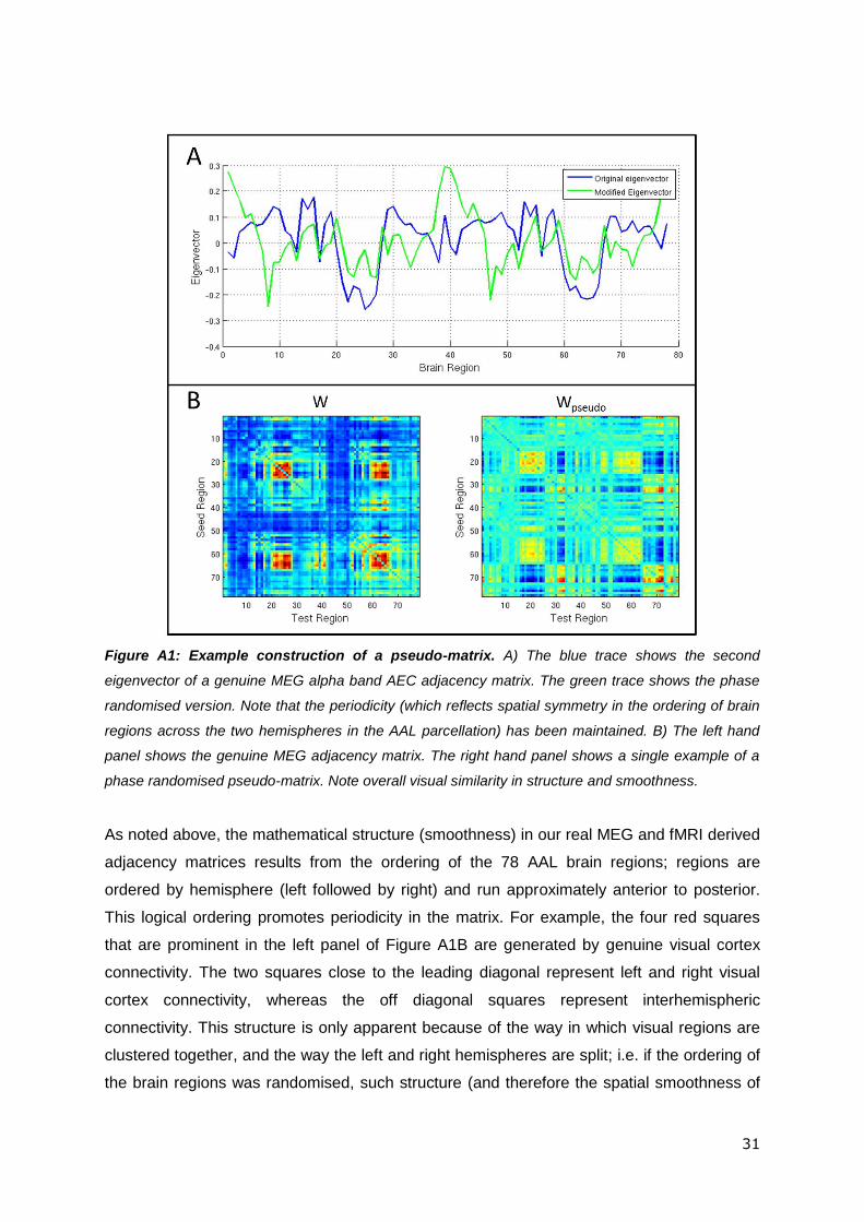
Figure A1: Example construction of a pseudo-matrix. A) The blue trace shows the second
eigenvector of a genuine MEG alpha band AEC adjacency matrix. The green trace shows the phase
randomised version. Note that the periodicity (which reflects spatial symmetry in the ordering of brain
regions across the two hemispheres in the AAL parcellation) has been maintained. B) The left hand
panel shows the genuine MEG adjacency matrix. The right hand panel shows a single example of a
phase randomised pseudo-matrix. Note overall visual similarity in structure and smoothness.
As noted above, the mathematical structure (smoothness) in our real MEG and fMRI derived
adjacency matrices results from the ordering of the 78 AAL brain regions; regions are
ordered by hemisphere (left followed by right) and run approximately anterior to posterior.
This logical ordering promotes periodicity in the matrix. For example, the four red squares
that are prominent in the left panel of Figure A1B are generated by genuine visual cortex
connectivity. The two squares close to the leading diagonal represent left and right visual
cortex connectivity, whereas the off diagonal squares represent interhemispheric
connectivity. This structure is only apparent because of the way in which visual regions are
clustered together, and the way the left and right hemispheres are split; i.e. if the ordering of
the brain regions was randomised, such structure (and therefore the spatial smoothness of
32
the matrix) would be destroyed. In the phase randomisation approach, the periodicity (hence
smoothness) in the genuine eigenvector shown in Figure 1A (blue trace) (which results from
the cross hemisphere split in the AAL region ordering) is mimicked in the phase randomised
eigenvector (green trace). This is because the amplitudes of the Fourier components of the
eigenvector are maintained. However, the precise brain regions involved differ. Application
of this approach to all eigenvectors means that the spatial smoothness and periodicity,
inherent to the genuine MEG matrices, is also apparent in the pseudo-matrices. However
any genuine connectivity information is destroyed making them appropriate for null
distribution calculation.
8) Acknowledgements
This work was funded by a Medical Research Council New Investigator Research Grant
(MR/M006301/1) awarded to MJB. We also acknowledge Medical Research Council
Partnership Grant (MR/K005464/1). The Anne McLaren Fellowship programme has funded
MGB.
Data used were collected as part of the University of Nottingham Multimodal Imaging Study
in Psychosis. We therefore express our thanks to all those involved in data collection,
particularly Emma Hall and Jyothika Kumar. The work on the second dataset was partially
supported by a private sponsorship to the VUmc MS center Amsterdam. The VUmc MS
centre Amsterdam is sponsored through a program grant by the Dutch MS Research
Foundation (grant number 09-358d). We thank Menno Schoonheim for acquisition and pre-
processing of fMRI dataset 2. We especially thank Cornelis J. Stam for his feedback and
input that improved the paper.
33
9) REFERENCES
Aru, J., Aru, J., Priesemann, V., Wibral, M., Lana, L., Pipa, G., Singer, W., Vicente, R., 2015. Untangling cross-frequency coupling in neuroscience. Current opinion in neurobiology 31, 51-61.
Ashburner, J., Andersson, J.L., Friston, K.J., 1999. High-dimensional image registration using symmetric priors. Neuroimage 9, 619-628.
Baker, A.P., Brookes, M.J., Rezek, I.A., Smith, S.M., Behrens, T., Smith, P.J.P., Woolrich, M., 2014. Fast transient networks in spontaneous human brain activity. Elife 3, e01867.
Birn, R.M., Murphy, K., Bandettini, P.A., 2008. The effect of respiration variations on independent component analysis results of resting state functional connectivity. Human brain mapping 29, 740-750.
Brookes, M.J., Gibson, A.M., Hall, S.D., Furlong, P.L., Barnes, G.R., Hillebrand, A., Singh, K.D., Holliday, I.E., Francis, S.T., Morris, P.G., 2005. GLM-beamformer method demonstrates stationary field, alpha ERD and gamma ERS co-localisation with fMRI BOLD response in visual cortex. Neuroimage 26, 302-308.
Brookes, M.J., Hale, J.R., Zumer, J.M., Stevenson, C.M., Francis, S.T., Barnes, G.R., Owen, J.P., Morris, P.G., Nagarajan, S.S., 2011a. Measuring functional connectivity using MEG: methodology and comparison with fcMRI. Neuroimage 56, 1082-1104.
Brookes, M.J., Liddle, E.B., Hale, J.R., Woolrich, M.W., Luckhoo, H., Liddle, P.F., Morris, P.G., 2012a. Task induced modulation of neural oscillations in electrophysiological brain networks. Neuroimage 63, 1918-1930.
Brookes, M.J., Mullinger, K.J., Stevenson, C.M., Morris, P.G., Bowtell, R., 2008. Simultaneous EEG source localisation and artifact rejection during concurrent fMRI by means of spatial filtering. NeuroImage, 1090-1104
Brookes, M.J., Woolrich, M., Luckhoo, H., Price, D., Hale, J.R., Stephenson, M.C., Barnes, G.R., Smith, S.M., Morris, P.G., 2011b. Investigating the electrophysiological basis of resting state networks using magnetoencephalography. Proceedings of the National Academy of Sciences 108, 16783-16788.
Brookes, M.J., Woolrich, M.W., Barnes, G.R., 2012b. Measuring functional connectivity in MEG: a multivariate approach insensitive to linear source leakage. Neuroimage 63, 910-920.
Brown, J.W., Churchill, R.V., Lapidus, M., 1996. Complex variables and applications. McGraw-Hill New York.
Bullmore, E., Sporns, O., 2009. Complex brain networks: graph theoretical analysis of structural and functional systems. Nature Reviews Neuroscience 10, 186-198.
Byrd, R.H., Schnabel, R.B., Shultz, G.A., 1987. A trust region algorithm for nonlinearly constrained optimization. SIAM Journal on Numerical Analysis 24, 1152-1170.
de Pasquale, F., Della Penna, S., Snyder, A.Z., Lewis, C., Mantini, D., Marzetti, L., Belardinelli, P., Ciancetta, L., Pizzella, V., Romani, G.L., 2010. Temporal dynamics of spontaneous MEG activity in brain networks. Proceedings of the National Academy of Sciences 107, 6040-6045.
de Pasquale, F., Della Penna, S., Snyder, A.Z., Marzetti, L., Pizzella, V., Romani, G.L., Corbetta, M., 2012. A cortical core for dynamic integration of functional networks in the resting human brain. Neuron 74, 753-764.
Deco, G., Jirsa, V.K., McIntosh, A.R., 2011. Emerging concepts for the dynamical organization of resting-state activity in the brain. Nature Reviews Neuroscience 12, 43-56.
34
Engel, A.K., Fries, P., Singer, W., 2001. Dynamic predictions: oscillations and synchrony in top–down processing. Nature Reviews Neuroscience 2, 704-716.
Engel, A.K., Gerloff, C., Hilgetag, C.C., Nolte, G., 2013. Intrinsic coupling modes: multiscale interactions in ongoing brain activity. Neuron 80, 867-886.
Gong, G., He, Y., Concha, L., Lebel, C., Gross, D.W., Evans, A.C., Beaulieu, C., 2009. Mapping anatomical connectivity patterns of human cerebral cortex using in vivo diffusion tensor imaging tractography. Cerebral cortex 19, 524-536.
Hall, E.L., Robson, S.E., Morris, P.G., Brookes, M.J., 2014. The relationship between MEG and fMRI. Neuroimage 102, 80-91.
Hall, E.L., Woolrich, M.W., Thomaz, C.E., Morris, P.G., Brookes, M.J., 2013. Using variance information in magnetoencephalography measures of functional connectivity. Neuroimage 67, 203-212.
Hillebrand, A., Barnes, G.R., 2005. Beamformer analysis of MEG data. International review of neurobiology 68, 149-171.
Hillebrand, A., Barnes, G.R., Bosboom, J.L., Berendse, H.W., Stam, C.J., 2012. Frequency-dependent functional connectivity within resting-state networks: an atlas-based MEG beamformer solution. Neuroimage 59, 3909-3921.
Hillebrand, A., Tewarie, P., van Dellen , E., Yu , M., Carbo, E.W.S., Douw, L., Gouw, A.A., van Straaten, E.C.W., Stam, C., 2015. Direction of information flow in large-scale resting-state networks is frequency dependent. submitted.
Hipp, J.F., Hawellek, D.J., Corbetta, M., Siegel, M., Engel, A.K., 2012. Large-scale cortical correlation structure of spontaneous oscillatory activity. Nature neuroscience 15, 884-890.
Hipp, J.F., Siegel, M., 2015. BOLD fMRI Correlation Reflects Frequency-Specific Neuronal Correlation. Current Biology.
Huang, M.X., Mosher, J.C., Leahy, R.M., 1999. A sensor-weighted overlapping-sphere head model and exhaustive head model comparison for MEG. Physics in Medicine and Biology 44, 423-440.
Hutchison, R.M., Womelsdorf, T., Allen, E.A., Bandettini, P.A., Calhoun, V.D., Corbetta, M., Della Penna, S., Duyn, J.H., Glover, G.H., Gonzalez-Castillo, J., 2013. Dynamic functional connectivity: promise, issues, and interpretations. Neuroimage 80, 360-378.
Jensen, O., Colgin, L.L., 2007. Cross-frequency coupling between neuronal oscillations. Trends in cognitive sciences 11, 267-269.
Kollo, T., von Rosen, D., 2006. Advanced multivariate statistics with matrices. Springer Science & Business Media.
Larson-Prior, L.J., Oostenveld, R., Della Penna, S., Michalareas, G., Prior, F., Babajani-Feremi, A., Schoffelen, J.-M., Marzetti, L., de Pasquale, F., Di Pompeo, F., 2013. Adding dynamics to the Human Connectome Project with MEG. Neuroimage 80, 190-201.
Liljeström, M., Stevenson, C., Kujala, J., Salmelin, R., 2015. Task-and stimulus-related cortical networks in language production: Exploring similarity of MEG-and fMRI-derived functional connectivity. Neuroimage.
Logothetis, N.K., 2003. The underpinnings of the BOLD functional magnetic resonance imaging signal. The Journal of Neuroscience 23, 3963-3971.

35
Luckhoo, H., Hale, J.R., Stokes, M.G., Nobre, A.C., Morris, P.G., Brookes, M.J., Woolrich, M.W., 2012. Inferring task-related networks using independent component analysis in magnetoencephalography. Neuroimage 62, 530-541.
Mantini, D., Perrucci, M.G., Del Gratta, C., Romani, G.L., Corbetta, M., 2007. Electrophysiological signatures of resting state networks in the human brain. Proceedings of the National Academy of Sciences 104, 13170-13175.
Meier, J., Tewarie, P., Hillebrand, A., Douw, L., van Dijk, B., Stufflebeam, S.M., van Mieghem, P., 2016. A mapping between structural and functional brain networks. submitted.
Menon, V., Ford, J.M., Lim, K.O., Glover, G.H., Pfefferbaum, A., 1997. Combined event‐related fMRI and EEG evidence for temporal—parietal cortex activation during target detection. Neuroreport 8, 3029-3037.
Mullinger, K.J., Mayhew, S.D., Bagshaw, A.P., Bowtell, R., Francis, S.T., 2013. Poststimulus undershoots in cerebral blood flow and BOLD fMRI responses are modulated by poststimulus neuronal activity. Proceedings of the National Academy of Sciences 110, 13636-13641.
Musso, F., Brinkmeyer, J., Mobascher, A., Warbrick, T., Winterer, G., 2010. Spontaneous brain activity and EEG microstates. A novel EEG/fMRI analysis approach to explore resting-state networks. Neuroimage 52, 1149-1161.
Nichols, T.E., Holmes, A.P., 2002. Nonparametric permutation tests for functional neuroimaging: a primer with examples. Human brain mapping 15, 1-25.
O'Neill, G.C., Bauer, M., Woolrich, M.W., Morris, P.G., Barnes, G.R., Brookes, M.J., 2015. Dynamic recruitment of resting state sub-networks. Neuroimage 115, 85-95.
Prichard, D., Theiler, J., 1994. Generating surrogate data for time series with several simultaneously measured variables. Physical Review Letters 73, 951.
Robinson, S.E., Mandell, A.J., Coppola, R., 2012. Spatiotemporal imaging of complexity. Frontiers in Computational Neuroscience, doi: 10.3389/fncom.2012.00101.
Sarvas, J., 1987. Basic mathematical and electromagnetic concepts of the biomagnetic inverse problem. Physics in Medicine and Biology 32, 11 - 22.
Schölvinck, M.L., Leopold, D.A., Brookes, M.J., Khader, P.H., 2013. The contribution of electrophysiology to functional connectivity mapping. Neuroimage 80, 297-306.
Singh, K.D., 2012. Which “neural activity” do you mean? fMRI, MEG, oscillations and neurotransmitters. Neuroimage 62, 1121-1130.
Singh, K.D., Barnes, G.R., Hillebrand, A., Forde, E.M., Williams, A.L., 2002. Task-related changes in cortical synchronization are spatially coincident with the hemodynamic response. Neuroimage 16, 103-114.
Smith, S.M., 2002. Fast robust automated brain extraction. Human brain mapping 17, 143-155.
Smith, S.M., Jenkinson, M., Woolrich, M.W., Beckmann, C.F., Behrens, T.E., Johansen-Berg, H., Bannister, P.R., De Luca, M., Drobnjak, I., Flitney, D.E., 2004. Advances in functional and structural MR image analysis and implementation as FSL. Neuroimage 23, S208-S219.
Stam, C.J., Nolte, G., Daffertshofer, A., 2007. Phase lag index: assessment of functional connectivity from multi channel EEG and MEG with diminished bias from common sources. Human brain mapping 28, 1178-1193.
36
Stevenson, C.M., Wang, F., Brookes, M.J., Zumer, J.M., Francis, S.T., Morris, P.G., 2012. Paired pulse depression in the somatosensory cortex: associations between MEG and BOLD fMRI. Neuroimage 59, 2722-2732.
Tewarie, P., Hillebrand, A., van Dellen, E., Schoonheim, M., Barkhof, F., Polman, C., Beaulieu, C., Gong, G., van Dijk, B., Stam, C., 2014. Structural degree predicts functional network connectivity: A multimodal resting-state fMRI and MEG study. Neuroimage 97, 296-307.
Tewarie, P., Schoonheim, M.M., Schouten, D.I., Polman, C.H., Balk, L.J., Uitdehaag, B.M., Geurts, J.J., Hillebrand, A., Barkhof, F., Stam, C.J., 2015. Functional brain networks: linking thalamic atrophy to clinical disability in multiple sclerosis, a multimodal fMRI and MEG study. Human brain mapping 36, 603-618.
Tzourio-Mazoyer, N., Landeau, B., Papathanassiou, D., Crivello, F., Etard, O., Delcroix, N., Mazoyer, B., Joliot, M., 2002. Automated anatomical labeling of activations in SPM using a macroscopic anatomical parcellation of the MNI MRI single-subject brain. Neuroimage 15, 273-289.
Van Mieghem, P., 2010. Graph spectra for complex networks. Cambridge University Press.
Wens, V., Bourguignon, M., Goldman, S., Marty, B., Op de Beeck, M., Clumeck, C., Mary, A., Peigneux, P., Van Bogaert, P., Brookes, M.J., De Tiege, X., 2014. Inter- and Intra-Subject Variability of Neuromagnetic Resting State Networks. Brain Topogr.


