Physica A 392 (2013) 3441–3458
Contents lists available at SciVerse ScienceDirect
Physica A
journal homepage: www.elsevier.com/locate/physa
Pricing currency options in the mixed fractionalBrownian motionLin Sun ∗
School of Applied Mathematics, Guangdong University of Technology, Guangzhou, 510520, PR China
h i g h l i g h t s
• A pricing model for currency options in mixed fractional Brownian motions is provided.• Some Greeks and the estimator of volatility are also presented.• Empirical studies show that the proposed model is a reasonable one.
a r t i c l e i n f o
Article history:Received 3 December 2012Received in revised form 25 January 2013Available online 17 April 2013
Keywords:Mixed fractional Brownian motionQuasi-conditional expectationCurrency optionOption pricing
a b s t r a c t
This paper deals with the problem of pricing European currency options in the mixedfractional Brownian environment. Both the pricing formula and themixed fractional partialdifferential equation for European call currency options are obtained. Some Greeks and theestimator of volatility are also provided. Empirical studies and simulation results confirmthe theoretical findings and show that the mixed fractional Brownian pricing model is areasonable one.
© 2013 Elsevier B.V. All rights reserved.
1. Introduction
A currency option is a contract, which gives the owner the right, but not the obligation, to buy or sell the indicatedamount of foreign currency at a specified price within a specified period of time (American Option) or on a fixed date(European Option). Since the currency option can be used as a tool for investment and hedging, it is one of the best tools forcorporations or individuals to hedge against adverse movements in exchange rates, and the theoretical models for pricingcurrency options have been carried out.
The valuationmodel for European currency options was presented by Garman and Kohlhagen (G–K hereafter) [1]. In fact,G–K is considered the biggest success in pricing currency options both in theory and in applicability. Its biggest strengthis the possibility of estimating market volatility of an underlying asset generally as a function of price and time withoutdirect reference to specific investor characteristics like expected yield, risk aversionmeasures or utility functions. Its secondstrongest strength aspect is self replicating strategy or hedging. Despite its usefulness and popularity, however, the G–Ktheory entails some inconsistencies. It is well known that the model frequently misprices deep in-the-money and deep out-of-the-money currency options (see Ref. [2]). The reasons for this mispricing is that the G–Kmodel is built on some non-reallife assumptions about the market: (i) volatility is a constant over time; (ii) returns of log normally distributed underlyingassets are normally distributed; (iii) both the domestic and foreign riskfree rates are constants; (iv) markets are perfectly
∗ Tel.: +86 136 624 31136.E-mail addresses: [email protected], [email protected].
0378-4371/$ – see front matter© 2013 Elsevier B.V. All rights reserved.http://dx.doi.org/10.1016/j.physa.2013.03.055
3442 L. Sun / Physica A 392 (2013) 3441–3458
liquid and it is possible to purchase or sell any amount of stock or options or their fractions at any given time. Among theselimitations, themost important reasonwhy thismodelmay not be entirely satisfactory could be that currencies are differentfrom stocks in important respects, and the geometric Brownianmotion cannot capture the behavior of currency returns (seeRef. [3]). Since then, in order to avoid this drawback, many methodologies for pricing currency options have been proposedby using modifications of the G–K model, such as Refs. [4,5].
All this research above assumes that the logarithmic returns of the exchange rate are independent identically distributednormal random variables. However, in general, the assumptions of the Gaussianity and mutual independence of underlyingasset log returns would not hold. Moreover, the empirical research has also shown that the distributions of the logarithmicreturns in the financial market usually exhibit excess kurtosis with more probability mass near the origin and in the tailsand less in the flanks than would occur for normally distributed data (see Ref. [6]). That is to say the distributions of thelogarithmic returns of financial assets usually exhibit properties of self-similarity, heavy tails, long-range dependence inboth auto-correlations and cross-correlations, and volatility clustering [7–24]. In this situation, it is possible to use one ofthe fractal processes, namely fractional Brownian motion, to describe these phenomena [25–32]. However, the fractionalBrownian motion is neither a Markov process nor a semi-martingale (except in the Brownian motion case), and we cannotuse the usual stochastic calculus to analyze it. Although some research have testified that the purely fractional Black–Scholesmarket becomes arbitrage-free withWick-self-financing strategies (see Refs. [33,34]), Björk and Hult [35] showed recently,that the use of fractional Brownian motion in finance does not make much economic sense because, while Wick integrationleads to no-arbitrage, the definition of the corresponding self-financing trading strategies is quite restrictive and, forexample, in the setup of Ref. [36], the simple buy-and-hold strategy is not self-financing. Thus, the fractional market basedonWick integrals is considered a beautiful mathematical construct but with limited applicability in finance. From the aboveanalyses, it is quite evident that the classical Itô theory could not apply to fractional Brownianmotion and defining a suitablestochastic integral with respect to fractional Brownian motion is difficult. Actually, the main problem of applying fractionalBrownianmotion in finance is that fBm is not a semi-martingale. To get around this problemand to take into account the longmemory property, it is reasonable to use the mixed fractional Brownian motion (mfBm hereafter) to capture fluctuations ofthe financial asset (see Refs. [37,38]).
The mfBm is a family of Gaussian processes that is a linear combination of Brownian motion and fractional Brownianmotion. It is one special class of long memory processes when Hurst parameter H > 1/2. In economics the first work to usefractional Brownian motion was [39]. Cheridito [39] has proved that, for H ∈ (3/4, 1), the mixed model with dependentBrownianmotion and fractional Brownianmotion is equivalent to onewith Brownianmotion, and hence it is arbitrage-free.Recent additional applications have been documented in Ref. [38]. Recently, the paper [29] considers the problem of pricingequity warrants in mfBm. Since the publication of this beautiful paper, the mfBm has subsequently become a standardmethodology to capture the fluctuations of asset prices. Following the ideal of Refs. [39,29] throughout this paper, we shallassume that H ∈ (3/4, 1). Actually, some empirical studies have verified that this assumption is valid [40–45]. Althoughseveral warrant pricing models have been discussed in a warrant pricing context, applying mfBm to price currency optionshas not been done. In this paper, to capture the long-range dependence of interest rates [46] and to exclude the arbitrage inthe environment of fractional Brownian motion, we consider the problem of pricing currency options in mfBm.
The remainder of this paper is organized as follows. In Section 2, we briefly state the formal definitions and propertiesrelated to mfBm that will be used in the forthcoming sections. In Section 3, we prove some results regarding the quasi-conditional expectation. In Section 4, we provide an analytic pricing formula for the European foreign currency options inmfBm. Section 5 dealswith themixed fractional partial differential equation and discusses someGreeks of thismixedmodel.In order to apply our model into realistic contexts, the estimator of volatility parameter, which is required in our pricingmodel, is also addressed in the latter part of this section. Section 6 is devoted to empirical studies and simulations to showthe performance of the mfBmmodel. Section 7 draws the concluding remarks. Some technical details and the pricing modelin pure fractional Brownian environment are presented in the Appendix.
2. Preliminaries
In this section we will present some definitions and results that we will need for the rest of the paper. These results canbe found in the fundamental papers concerning the mfBm and fractional Itô integral: [47,48,39,49,38].
Definition 2.1. Amixed fractional Brownianmotion of parameters α, β andH is a linear combination of different fractionalBrownian motions, defined on the probability space (Ω,F , P) for any t ∈ R+ by:
MHt = αBt + βBH
t , (2.1)
where Bt is a Brownian motion, BHt is an independent fractional Brownian motion of Hurst parameter H ∈ (0, 1), α and β
are two real constants such that (α, β) = (0, 0).
Now recalling the results in Refs. [49,29], we shall present some properties by the following proposition.
Proposition 2.2. The mfBm MHt satisfies the following properties:
(i) MHt is a centered Gaussian process and not a Markovian one for all H ∈ (0, 1) \ 1/2;
L. Sun / Physica A 392 (2013) 3441–3458 3443
(ii) MH0 = 0 P-almost surely;
(iii) the covariation function of MHt (α, β) and MH
s (a, b) for any t, s ∈ R+ is given by
Cov(MHt ,M
Hs ) = α2(t ∧ s)+
β2
2(t2H + s2H − |t − s|2H);
(iv) the increments of MHt (α, β) are stationary and mixed-self-similar for any h > 0
MHht(α, β) , MH
t
αh
12 , βhH
,
where , means ‘‘to have the same law’’;(v) the increments of MH
t are positively correlated if 12 < H < 1, uncorrelated if H =
12 and negatively correlated if
0 < H < 12 ;
(vi) the increments of MHt are long-range dependent if, and only if H > 1
2 ;(vii) for all t ∈ R+
E[(MHt (α, β))
n] =
0, n = 2l + 1,(2l)!2ll!
(α2t + β2t2H)l, n = 2l.(2.2)
Proof. These properties are easily obtained based on Refs. [29,49].
It is obvious to conclude that secondmoment as well as increments correlation function can be used for anti-persistenceor long-range dependences detection.
3. Some relative results regarding the quasi-conditional expectation
In this section, we present some result regarding the quasi-conditional expectation that we will need for the rest of thepaper (see also in Ref. [29]). Now, let (Ω,F , P) be a probability field such that Bt is a Brownian motion with respect to Pand BH
t is an independent fractional Brownian motion with respect to P.
Lemma 3.1. For every 0 < t < T and σ ∈ C, we have
Et
eσBT+BHT
= eσ
Bt+BHt
+σ22 (T−t)+ σ2
2 (T2H
−t2H ), (3.1)
where Et denotes the quasi-conditional expectation with respect to the risk-neutral measure.
Lemma 3.2. Let f be a function such that Et [f (BT , BHT )] < ∞. Then for every 0 < t ≤ T and σ ∈ C,
EtfσBT + σBH
T
=
R
12π [σ 2(T − t + T 2H − t2H)]
exp
−
(x − σBt − σBHt )
2
2σ 2(T − t + T 2H − t2H)
f (x)dx.
Let f (x) = 1A(x). We can easily obtain the following corollary.
Corollary 3.3. Let A ∈ B(R). Then
Et [1A(σBT + σBHT )] =
R
12π [σ 2(T − t + T 2H − t2H)]
exp
−
(x − σBt − σBHt )
2
2σ 2(T − t + T 2H − t2H)
1A(x)dx.
Let θ, ω ∈ R. Now, we consider the process
Z∗
t = θB∗
t + ω(BHt )
∗= θBt + θ2t + ωBH
t + ω2t2H , 0 ≤ t ≤ T .
From the Girsanov theorem, there exists a measure P∗ such that Z∗t is a mfBm.Wewill denote E∗
t [·] the quasi-conditionalexpectation with respect to P∗. Consider
Xt = exp
−θBt −θ2
2t − ωBH
t −ω2
2t2H.
3444 L. Sun / Physica A 392 (2013) 3441–3458
Lemma 3.4. Let f be a function such that Et [f (θBT + ωBHT )] < ∞. Then for every t ≤ T ,
E∗
t [f (θBT + ωBHT )] =
1Xt
Et [f (θBT + ωBHT )XT ].
Theorem 3.5. The price at every t ∈ [0, T ] of a bounded FHT -measurable claim F ∈ L2 is given by
Ft = e−r(T−t)Et [F ],
where r represents the constant riskless interest rate.
4. The pricing model of currency options
The purpose of this section is to derive the pricing formula for a European option. The mixed fractional Black–Scholesequation is obtained and the sensitivity indicators are also analyzed in the latter part of this section.
Now consider a mixed fractional Black–Scholes currency market that has two investment possibilities:(i) a money market account:
dPt = rdPtdt, P0 = 1, 0 ≤ t ≤ T , (4.1)
where rd represents the domestic interest rate.(ii) a stock whose price satisfies the equation:
dSt = µStdt + σ StdBt + σ StdBHt , S0 = S > 0, 0 ≤ t ≤ T , (4.2)
where H is Hurst parameter satisfied H > 3/4.Making the change of variable Bt + BH
t =µ+rf −rd
σ+ Bt + BH
t , then under the risk-neutral measure we have that:
dSt = (rd − rf )Stdt + σ StdBt + σ StdBHt , S0 = S > 0, 0 ≤ t ≤ T , (4.3)
where rf is the foreign interest rate.Hence we obtain the solution of (4.3)
St = S0 exp
rd − rft + σ
Bt + BH
t
−
12σ 2t −
12σ 2t2H
. (4.4)
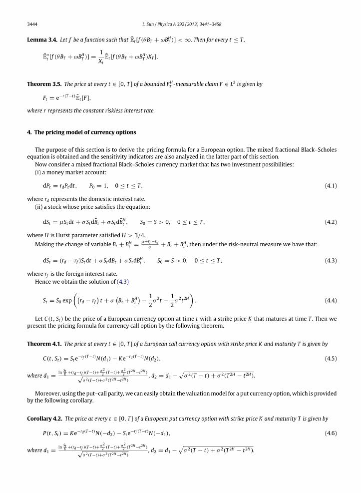
Let C(t, St) be the price of a European currency option at time t with a strike price K that matures at time T . Then wepresent the pricing formula for currency call option by the following theorem.
Theorem 4.1. The price at every t ∈ [0, T ] of a European call currency option with strike price K and maturity T is given by
C(t, St) = Ste−rf (T−t)N(d1)− Ke−rd(T−t)N(d2), (4.5)
where d1 =ln St
K +(rd−rf )(T−t)+ σ22 (T−t)+ σ2
2 (T2H
−t2H )√σ 2(T−t)+σ 2(T2H−t2H )
, d2 = d1 −σ 2(T − t)+ σ 2(T 2H − t2H).
Moreover, using the put–call parity, we can easily obtain the valuationmodel for a put currency option, which is providedby the following corollary.
Corollary 4.2. The price at every t ∈ [0, T ] of a European put currency option with strike price K and maturity T is given by
P(t, St) = Ke−rd(T−t)N(−d2)− Ste−rf (T−t)N(−d1), (4.6)
where d1 =ln St
K +(rd−rf )(T−t)+ σ22 (T−t)+ σ2
2 (T2H
−t2H )√σ 2(T−t)+σ 2(T2H−t2H )
, d2 = d1 −σ 2(T − t)+ σ 2(T 2H − t2H).
L. Sun / Physica A 392 (2013) 3441–3458 3445
5. Comparative statics analysis
Suppose that we have a currency option whose value V (t, St) depends only on t and St . It is not necessary at this stage tospecify whether V is a call or a put; indeed, V can be the value of a whole portfolio of different options. Then we shall statethe mixed fractional Black–Scholes partial differential equation by the following theorem.
Theorem 5.1. The price of a currency option with a bounded payoff f (ST ) is given by V (t, St)where V (t, S) is the solution of thePDE:
∂V∂t
+12σ 2S2
∂2V∂S2
+ Hσ 2t2H−1S2∂2V∂S2
+ (rd − rf )S∂V∂S
− rdV = 0.
After establishing the formula to calculate the valuation of currency options, in what follows, we will turn to discussthe properties of this pricing formula. In finance, Greeks measure the sensitivity of the option prices to a change inunderlying parameters which are price of the asset, interest rate, volatility and time decay. Hence Greeks are vital toolsin risk management and trading options without the knowledge of Greeks can result in heavy losses. In what follows, wewill discuss Greeks of our pricing model in detail.
Theorem 5.2. The Greeks are given by
∆ =∂C∂S
= e−rf (T−t)N(d1),
∇ =∂C∂K
= −e−rd(T−t)N(d2),
ρrd =∂C∂rd
= (T − t)Ke−rd(T−t)N(d2),
ρrf =∂C∂rf
= (T − t)Se−rf (T−t)N(d1),
Θ =∂C∂t
= −rdKe−rd(T−t)N(d2)−12e−rf (T−t) σ 2
+ 2Hσ 2t2H−1σ 2(T − t)+ σ 2(T 2H − t2H)
StN ′(d1),
+ rf e−rf (T−t)StN(d1),
Γ =∂2C∂S2
= e−rf (T−t) N ′(d1)
Stσ 2(T − t)+ σ 2(T 2H − t2H)
,
ϑσ =∂C∂σ
= e−rf (T−t) StN ′(d1)σ (T − t)σ 2(T − t)+ σ 2(T 2H − t2H)
.
It is clear that our mfBmmodel depends on Hurst parameter H . Hence we present the influence of this parameter in thefollowing theorem.
Theorem 5.3. The influence of the Hurst parameter can be written as
∂C∂H
= Se−rf (T−t)N ′(d1)σ 2(T 2H ln T − t2H ln t)σ 2(T − t)+ σ 2(T 2H − t2H)
.
Comparing the G–K model with our mixed fractional currency model, we have the conclusion that the differentparameters, Hurst exponent and volatility, should be estimated. However, the estimation of H has been extensively studied.The simplest andmost popularmethod is the so-called R/S analysis. Hence, we shall just focus on the estimation of volatility.
Theorem 5.4. Let 0 ≤ T1 < T2 be given, and suppose we choose a partition of this interval, T1 = t0 < t1 < · · · < tn = T2. LetSti denote the time series of observed prices. Then the volatility of the interval [T1, T2] is given by
σ 2=
1T2 − T1 + TH
2 − TH1
n−1j=0
log
Stj+i
Stj
2
. (5.1)
3446 L. Sun / Physica A 392 (2013) 3441–3458
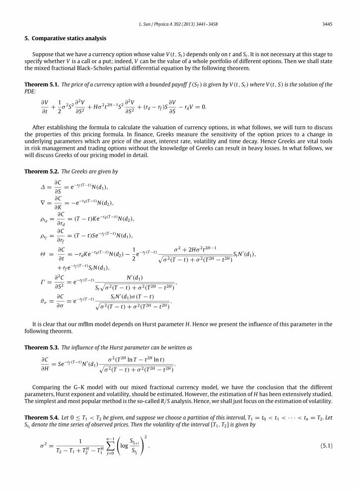
(a) Daily closing prices. (b) Daily log returns.
(c) Q–Q plot. (d) Probability density of the return.
Fig. 1. Some statistical figures of daily returns for the GBP/USD exchange rate from January 4th 2005 to March 15th 2006.
Table 1Summary statistics of the return for the GBP/USD exchange rate.
Minimum Maximum Median Mean Std. Dev. Skewness Kurtosis P-value
−0.016406 0.014957 −0.008110 −0.000265 0.005347 −0.191047 3.521724 0.0087
6. Implications for computing the valuation of currency option
After establishing the pricing model of currency options, in this section, for an illustration of the model derived inprevious sections, the proposed mfBm model is tested against the daily market price datum of China Merchant Bank’sGBP/USD call currency option. The data set used in the empirical application is the European currency call option for theBritish pound written on the US dollar, taken from the Website of China Merchant Bank. And the exchange rate quotationsutilized in our empirical investigation are extracted from the Wind Financial Database including GBP/USD spanning from01/04/2005 through 03/15/2006. Inwhat follows, wewill compute the call currency option prices using ourmodel andmakecomparisons with the results of existing valuation models.
Now,we turn to discuss the statistical properties of GBP/USD exchange rate. Fig. 1 provides some empirical data about theGBP/USD exchange rate. Specifically, Fig. 1(a) shows the daily closing values of GBP/USD exchange rate in the sample period.Fig. 1(b) illustrates the continuously compounded returns (the log returns) associated with the price series in Fig. 1(a). Incontrast to the price series in Fig. 1(a), the log returns appear to be quite stable over time. Fig. 1(c) presents the Q–Q figureduring the sample period. We can observe that the empirical distribution of log returns does in fact exhibit fat tails andclearly deviates from the normality assumption. From the visual evidence of a highly peaked and fat tailed distribution, wecan conclude that small and large movements in the empirical samples occur more likely compared to normally distributedlog returns.Moreover, the frequency distribution of daily log returns of the GBP/USD exchange rate during the sample periodis pictured in Fig. 1(d) and a normal distribution is depicted by the solid line. The empirical distributions are highly peakedcompared to the normal distribution.
To give a brief insight into the properties of the data and to find further evidence against the normality assumption,Table 1 tabulated the descriptive statistics of the return for the GBP/USD exchange rate in the sample period. The first,second, third, fourth and fifth columns contain the basic descriptive statistics for this time series. Moreover, Skewness,Kurtosis and P-value of Jarque–Bera test are also presented in this table.
Based on the sample kurtosis and skewnesswe test the null hypothesis that the data is drawn from a normal distribution.The null hypothesis is a joint hypothesis of the skewness being zero and the excess kurtosis being zero. The overall conclusionby looking into Table 1, when considering the full sample of log returns, is that we clearly reject the null hypothesis, that
L. Sun / Physica A 392 (2013) 3441–3458 3447
Sam
ple
Aut
ocor
rela
tion
–0.2
–0.15
–0.1
–0.05
0
0.05
0.1
0.15
0.2
0 5 10 15 20 25 30 35
Lag
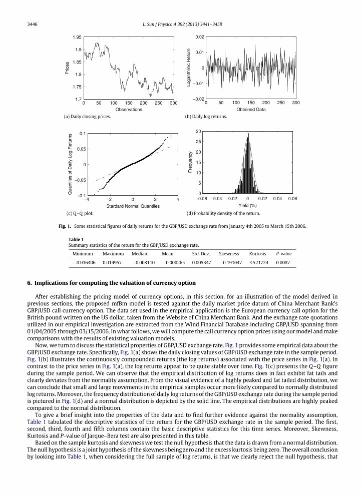
Fig. 2. The ACF plots of the returns of GBP/USD exchange rate from January 4th 2005 to March 15th 2006.
Table 2Results by different pricing models vs. actual market prices.
Exchange rate T − t PG–K PM–C PF–B PM–F PActual
1.213 0.214 0.02670 0.02668 0.02896 0.02955 0.030051.214 0.240 0.02728 0.02725 0.02901 0.03114 0.033491.215 0.250 0.02786 0.02783 0.02924 0.03246 0.034581.216 0.220 0.02846 0.02842 0.02955 0.03273 0.034591.217 0.195 0.02906 0.02910 0.03029 0.03330 0.032641.218 0.208 0.02966 0.02971 0.03103 0.03395 0.03360
the sample data of the GBP/USD exchange rate is from a normal distribution. This conclusion comes from the P-value ofJarque–Bera test. From Table 1, we can see that the P-value is below the default significance level of 5%. Hence we obtainthat the distribution of yield series is not a normal distribution, but a skew distribution.
In what follows, we turn to present an investigation of whether the GBP/USD exchange rate has long-range dependence.Fig. 2 plots the sample autocorrelation functions for the daily returns of GBP/USD exchange rate. From Fig. 2 we observe thatthe decay of autocorrelation function is veryweak. Thereforewemay obtain that the GBP/USD exchange rate has long-rangedependence.
Now, we present more information on the ChinaMerchant Bank’s GBP/USD call currency option. This was a three-monthcurrency call option with a strike price K = 1.21. The US and British risk-free interest rates are relatively stable over thesample period. The basic parameters are listed as follows: the 3-month volatility is about 9% using (5.1); the domestic 3-month is 4.93%; and the foreign 3-month interest rate is 2.71%. Based on the historical datum, we use the R/S analysismethodology to estimate the Hurst exponent H = 0.538. Next, we can compute the valuation of the GBP/USD call optionusing different pricing models with currency quotations lying in the closed interval of [1.213, 1.218]. The remaining timeto maturity T − t is updated according to the underlying asset. The results are presented in Table 2, where PActual denotesthe market price of GBP/USD currency option; PG–K denotes the price computed by the G–K model; PM–C denotes the pricesimulated by the Monte Carlo method; PF–B denotes the price computed according to the pure fBmmodel, and PM–F denotesthe price computed according to the mfBmmodel.
It is observed that the G–K model, the Monte Carlo simulation and the pure fBm model consistently underprice thecurrency option while the pricing results (the sixth column of Table 2) of formula (4.5) are closer to actual currency optionprices than the results of the other models. Furthermore, the complicated calculation of formula (4.5) can be computedeasily by a computer program. These factors indicate that our mfBm can capture the behavior of the exchange rate and ourcurrency pricing model has a good performance empirically.
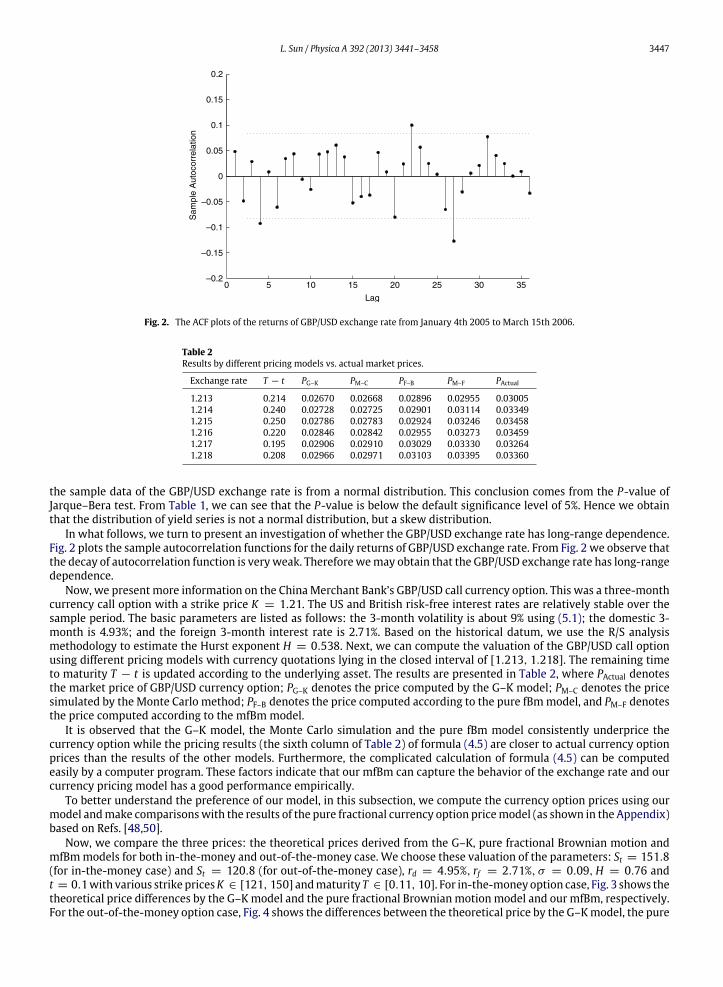
To better understand the preference of our model, in this subsection, we compute the currency option prices using ourmodel andmake comparisonswith the results of the pure fractional currency option pricemodel (as shown in the Appendix)based on Refs. [48,50].
Now, we compare the three prices: the theoretical prices derived from the G–K, pure fractional Brownian motion andmfBmmodels for both in-the-money and out-of-the-money case. We choose these valuation of the parameters: St = 151.8(for in-the-money case) and St = 120.8 (for out-of-the-money case), rd = 4.95%, rf = 2.71%, σ = 0.09,H = 0.76 andt = 0.1with various strike pricesK ∈ [121, 150] andmaturity T ∈ [0.11, 10]. For in-the-moneyoption case, Fig. 3 shows thetheoretical price differences by the G–Kmodel and the pure fractional Brownian motion model and our mfBm, respectively.For the out-of-the-money option case, Fig. 4 shows the differences between the theoretical price by the G–Kmodel, the pure
3448 L. Sun / Physica A 392 (2013) 3441–3458
Fig. 3. Relative difference among the G–K model, pure fBm model and mfBmmodel for the in-the-money case.
Fig. 4. Relative difference among the G–K model, pure fBm model and mfBmmodel for the out-the-money case.
fractional Brownianmotionmodel and ourmfBmmodel, respectively. In each figure, the vertical axis denotes the differencesbetween the two prices, and the horizontal axis denotes time to maturity and the strike price. These figures show that theprices by our mixed model are better fitted to the G–K prices than those by the pure fractional Brownian motion model forboth in-the-money and out-of-themoney cases. Hence,when compared to these figures, ourmfBmmodel seems reasonable.
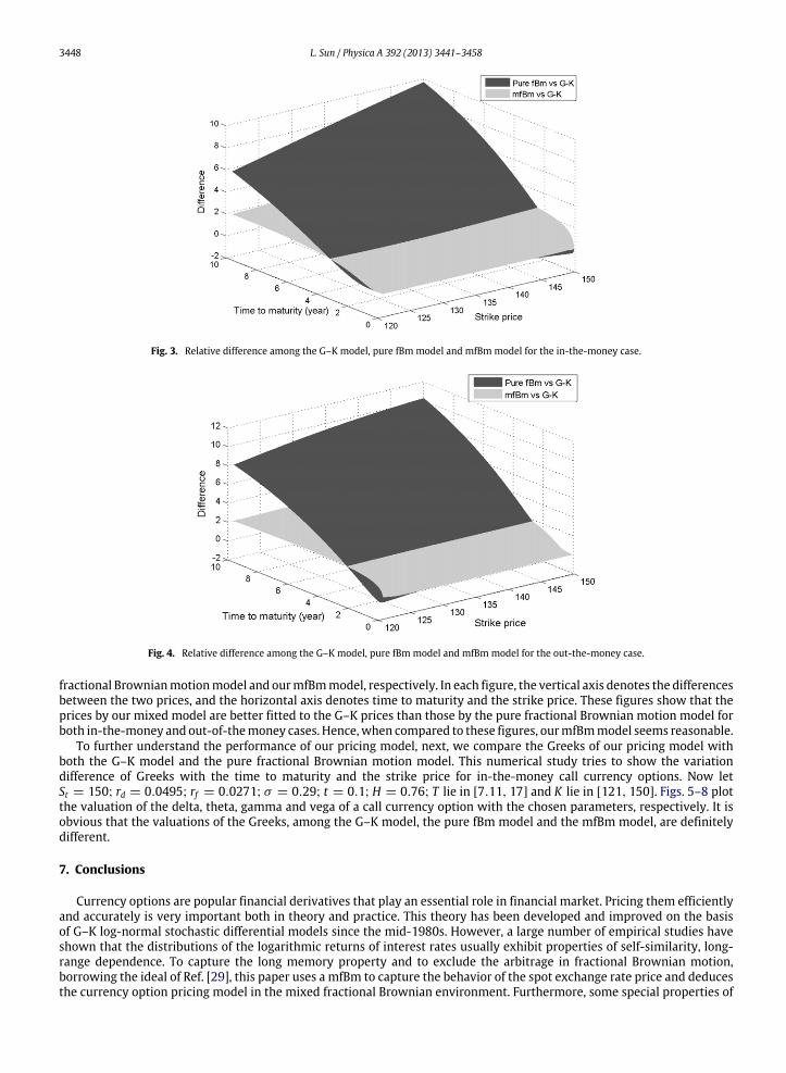
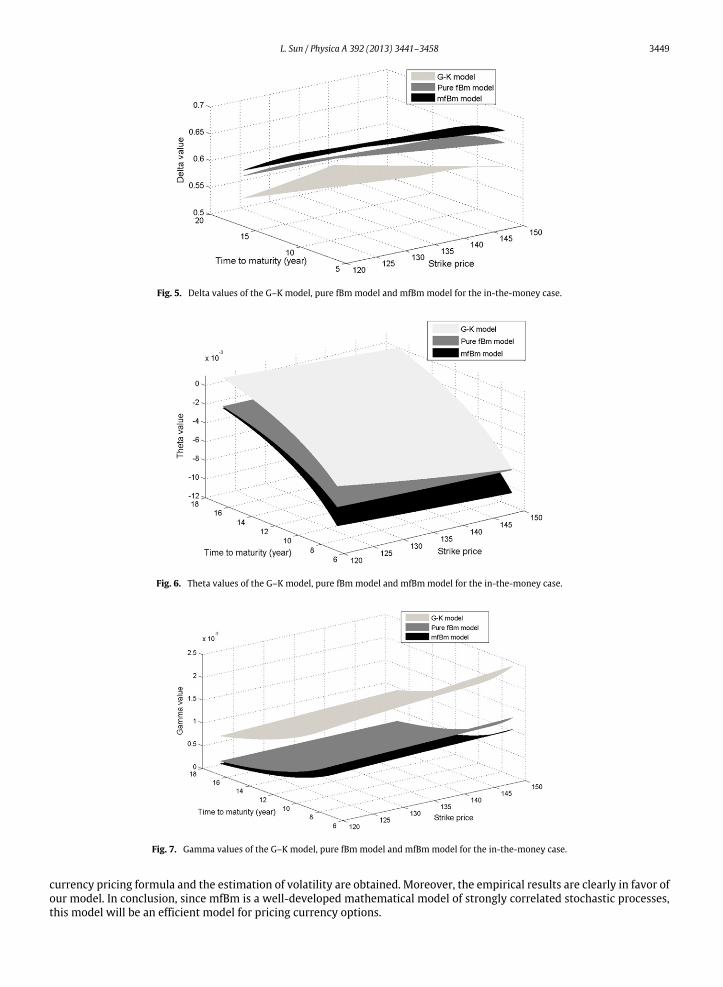
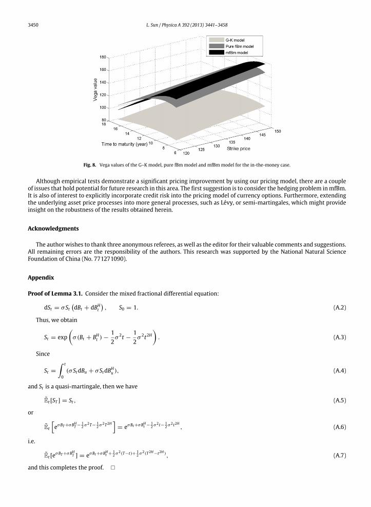
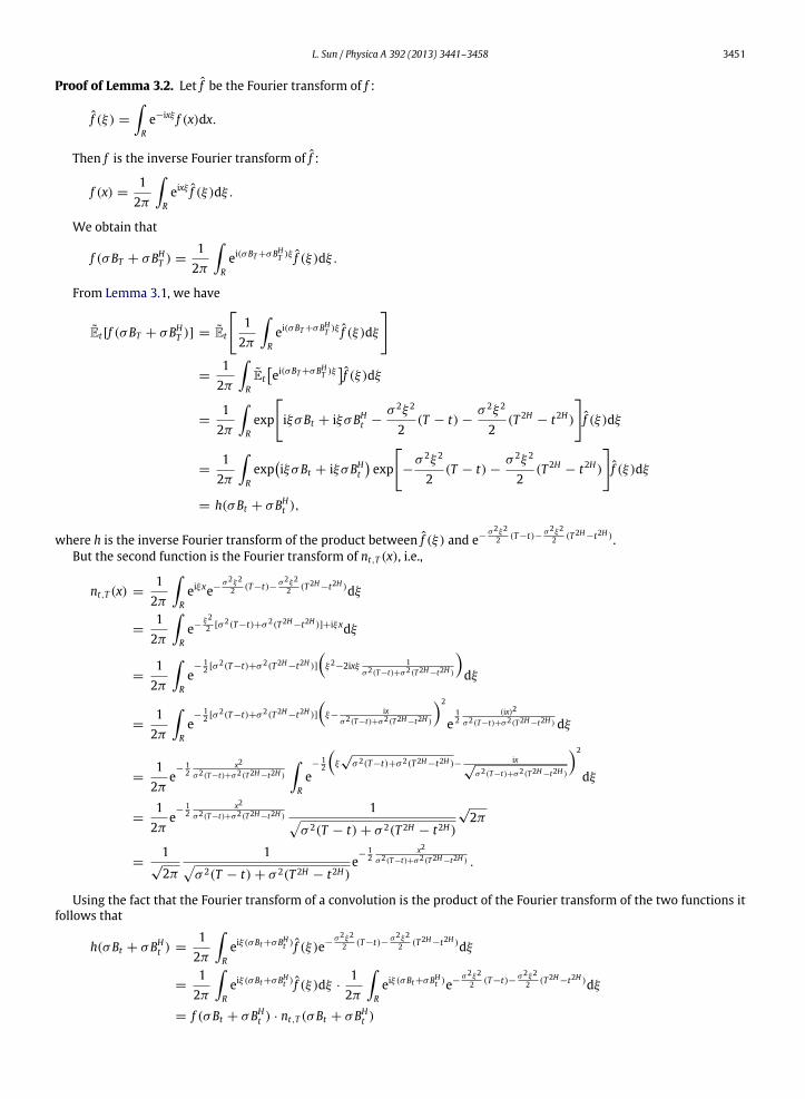
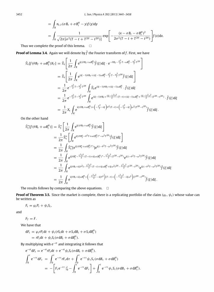
To further understand the performance of our pricing model, next, we compare the Greeks of our pricing model withboth the G–K model and the pure fractional Brownian motion model. This numerical study tries to show the variationdifference of Greeks with the time to maturity and the strike price for in-the-money call currency options. Now letSt = 150; rd = 0.0495; rf = 0.0271; σ = 0.29; t = 0.1;H = 0.76; T lie in [7.11, 17] and K lie in [121, 150]. Figs. 5–8 plotthe valuation of the delta, theta, gamma and vega of a call currency option with the chosen parameters, respectively. It isobvious that the valuations of the Greeks, among the G–K model, the pure fBm model and the mfBm model, are definitelydifferent.
7. Conclusions
Currency options are popular financial derivatives that play an essential role in financial market. Pricing them efficientlyand accurately is very important both in theory and practice. This theory has been developed and improved on the basisof G–K log-normal stochastic differential models since the mid-1980s. However, a large number of empirical studies haveshown that the distributions of the logarithmic returns of interest rates usually exhibit properties of self-similarity, long-range dependence. To capture the long memory property and to exclude the arbitrage in fractional Brownian motion,borrowing the ideal of Ref. [29], this paper uses a mfBm to capture the behavior of the spot exchange rate price and deducesthe currency option pricing model in the mixed fractional Brownian environment. Furthermore, some special properties of
L. Sun / Physica A 392 (2013) 3441–3458 3449
Fig. 5. Delta values of the G–K model, pure fBm model and mfBmmodel for the in-the-money case.
Fig. 6. Theta values of the G–K model, pure fBm model and mfBmmodel for the in-the-money case.
Fig. 7. Gamma values of the G–K model, pure fBm model and mfBmmodel for the in-the-money case.
currency pricing formula and the estimation of volatility are obtained. Moreover, the empirical results are clearly in favor ofour model. In conclusion, since mfBm is a well-developed mathematical model of strongly correlated stochastic processes,this model will be an efficient model for pricing currency options.
3450 L. Sun / Physica A 392 (2013) 3441–3458
Fig. 8. Vega values of the G–K model, pure fBm model and mfBmmodel for the in-the-money case.
Although empirical tests demonstrate a significant pricing improvement by using our pricing model, there are a coupleof issues that hold potential for future research in this area. The first suggestion is to consider the hedging problem inmfBm.It is also of interest to explicitly incorporate credit risk into the pricing model of currency options. Furthermore, extendingthe underlying asset price processes into more general processes, such as Lévy, or semi-martingales, which might provideinsight on the robustness of the results obtained herein.
Acknowledgments
The author wishes to thank three anonymous referees, as well as the editor for their valuable comments and suggestions.All remaining errors are the responsibility of the authors. This research was supported by the National Natural ScienceFoundation of China (No. 771271090).
Appendix
Proof of Lemma 3.1. Consider the mixed fractional differential equation:
dSt = σ StdBt + dBH
t
, S0 = 1. (A.2)
Thus, we obtain
St = expσ(Bt + BH
t )−12σ 2t −
12σ 2t2H
. (A.3)
Since
St =
t
0(σ StdBu + σ StdBH
u ), (A.4)
and St is a quasi-martingale, then we have
Et [ST ] = St , (A.5)
or
Et
eσBT+σBHT −
12 σ
2T−12 σ
2T2H
= eσBt+σBHt −
12 σ
2t− 12 σ
2t2H , (A.6)
i.e.
Et [eσBT+σBHT ] = eσBt+σBHt +
12 σ
2(T−t)+ 12 σ
2(T2H−t2H ), (A.7)
and this completes the proof.
L. Sun / Physica A 392 (2013) 3441–3458 3451
Proof of Lemma 3.2. Let f be the Fourier transform of f :
f (ξ) =
Re−ixξ f (x)dx.
Then f is the inverse Fourier transform of f :
f (x) =12π
Reixξ f (ξ)dξ .
We obtain that
f (σBT + σBHT ) =
12π
Rei(σBT+σBHT )ξ f (ξ)dξ .
From Lemma 3.1, we have
Et [f (σBT + σBHT )] = Et
12π
Rei(σBT+σBHT )ξ f (ξ)dξ
=12π
R
Etei(σBT+σBHT )ξ
f (ξ)dξ
=12π
Rexp
iξσBt + iξσBH
t −σ 2ξ 2
2(T − t)−
σ 2ξ 2
2(T 2H
− t2H)
f (ξ)dξ
=12π
Rexp
iξσBt + iξσBH
t
exp
−σ 2ξ 2
2(T − t)−
σ 2ξ 2
2(T 2H
− t2H)
f (ξ)dξ
= h(σBt + σBHt ),
where h is the inverse Fourier transform of the product between f (ξ) and e−σ2ξ2
2 (T−t)− σ2ξ22 (T2H−t2H ).
But the second function is the Fourier transform of nt,T (x), i.e.,
nt,T (x) =12π
Reiξxe−
σ2ξ22 (T−t)− σ2ξ2
2 (T2H−t2H )dξ
=12π
Re−
ξ22 [σ 2(T−t)+σ 2(T2H−t2H )]+iξxdξ
=12π
Re−
12 [σ 2(T−t)+σ 2(T2H−t2H )]
ξ2−2ixξ 1
σ2(T−t)+σ2(T2H−t2H )
dξ
=12π
Re−
12 [σ 2(T−t)+σ 2(T2H−t2H )]
ξ− ix
σ2(T−t)+σ2(T2H−t2H )
2
e12
(ix)2
σ2(T−t)+σ2(T2H−t2H ) dξ
=12π
e−
12
x2
σ2(T−t)+σ2(T2H−t2H )
Re−
12
ξ√σ 2(T−t)+σ 2(T2H−t2H )− ix√
σ2(T−t)+σ2(T2H−t2H )
2
dξ
=12π
e−
12
x2
σ2(T−t)+σ2(T2H−t2H )1
σ 2(T − t)+ σ 2(T 2H − t2H)
√2π
=1
√2π
1σ 2(T − t)+ σ 2(T 2H − t2H)
e−
12
x2
σ2(T−t)+σ2(T2H−t2H ) .
Using the fact that the Fourier transform of a convolution is the product of the Fourier transform of the two functions itfollows that
h(σBt + σBHt ) =
12π
Reiξ(σBt+σB
Ht ) f (ξ)e−
σ2ξ22 (T−t)− σ2ξ2
2 (T2H−t2H )dξ
=12π
Reiξ(σBt+σB
Ht ) f (ξ)dξ ·
12π
Reiξ(σBt+σB
Ht )e−
σ2ξ22 (T−t)− σ2ξ2
2 (T2H−t2H )dξ
= f (σBt + σBHt ) · nt,T (σBt + σBH
t )
3452 L. Sun / Physica A 392 (2013) 3441–3458
=
Rnt,T (σBt + σBH
t − y)f (y)dy
=
R
12π [σ 2(T − t + T 2H − t2H)]
exp
−
(x − σBt − σBHt )
2
2σ 2(T − t + T 2H − t2H)
f (x)dx.
Thus we complete the proof of this lemma.
Proof of Lemma 3.4. Again we will denote by f the Fourier transform of f . First, we have
Et [f (θBT + ωBHT )XT ] = Et
12π
Reiξ(θBT+ωBHT ) f (ξ)dξ · e−θBT−
θ22 T−ωBHT −
ω22 T2H
= Et
12π
Re(iξ−1)θBT+(iξ−1)ωBHT −
θ22 T−
ω22 T2H f (ξ)dξ
=12π
e−θ22 T−
ω22 T2H
R
Ete(iξ−1)θBT+(iξ−1)ωBHT · f (ξ)dξ
=12π
e−θ22 T−
ω22 T2H
Re(iξ−1)θBt+
(iξ−1)2θ22 (T−t)+(iξ−1)ωBHt +
(iξ−1)2ω22 (T2H−t2H )
· f (ξ)dξ
=12π
Xt
Reiξ(θBt+ωBHt )+
−ξ22 −iξ
θ2(T−t)+
−ξ22 −iξ
ω2(T2H−t2H )
f (ξ)dξ .
On the other hand
E∗
t [f (θBt + ωBHt )] = E∗
t
12π
Reiξ(θBT+ωBHT ) f (ξ)dξ
=
12π
E∗
t
Reiξ(θB
∗T−θ2T+ω(BHT )
∗−ω2T2H ) f (ξ)dξ
=
12π
R
E∗
t [eiξ(θB∗
T+ω(BHT )∗)
]eiξ(−θ2T−ω2T2H ) f (ξ)dξ
=12π
ReiξθB
∗t −
ξ2θ22 (T−t)+iξω(BHt )
∗−ξ2ω2
2 (T2H−t2H )eiξ(−θ2T−ω2T2H ) f (ξ)dξ
=12π
ReiξθBt+iξθ2t− ξ2θ2
2 (T−t)+iξωBHt +iξω2t2H−ξ2ω2
2 (T2H−t2H )eiξ(−θ2T−ω2T2H ) f (ξ)dξ
=12π
ReiξθBt+iξωBHt +
−ξ2θ2
2 −iξθ2(T−t)+
−ξ2ω2
2 −iξω2(T2H−t2H )
f (ξ)dξ .
The results follows by comparing the above equations.
Proof of Theorem 3.5. Since the market is complete, there is a replicating portfolio of the claim (ϕt , ψt) whose value canbe written as
Ft = ϕtPt + ψtSt ,
and
FT = F .
We have that
dFt = ϕt rPtdt + ψt(rStdt + σ StdBt + σ StdBHt )
= rFtdt + ψtSt(σdBt + σdBHt ).
By multiplying with e−rt and integrating it follows that
e−rtdFt = e−rt rFtdt + e−rtψtSt(σdBt + σdBHt ). t
0e−rτdFτ =
t
0e−rτ rFτdτ +
t
0e−rτψτ Sτ (σdBτ + σdBH
τ )
= −
Fτe−rτ
|t0 −
t
0e−rτdFτ
+
t
0e−rτψτ Sτ (σdBτ + σdBH
τ ).
L. Sun / Physica A 392 (2013) 3441–3458 3453
Consequently,
e−rtFt = F0 +
t
0e−rτψτ Sτ (σdBτ + σdBH
τ ). (A.8)
By the fractional Clark–Ocone theorem (see Ref. [38]) we have that
e−rtF = e−rT Et [F ] + e−rT T
0Eτ [Dτ F ](σdBτ + σdBH
τ ).
From the completeness of the market we get
Eτ [Dτ F ] = er(T−τ)ψτ Sτ .
So we have that
e−rtF = e−rT Et [F ] +
T
0e−rτψτ Sτ (σdBτ + σdBH
τ ).
It follows that
Et [e−rtF ] = e−rT Et [F ] + Et
T
0e−rτψτ Sτ (σdBτ + σdBH
τ )
.
Since T0 f (s, ω)(σdBτ + σdBH
τ ) is a quasi-Martingale, we have
Et [e−rtF ] = e−rT Et [F ] +
t
0e−rτψτ Sτ (σdBτ + σdBH
τ ). (A.9)
From (A.8) and (A.9), we obtain that
Ft = e−r(T−t)Et [F ].
Thus we complete the proof.
Proof of Theorem 4.1. Motivated from Theorem 3.5, a European call with maturity T and strike price K is theoreticallyequivalent to
C(t, St) = Et [e−rd(T−t)(ST − K)+]
= e−rd(T−t)EtST1[ST>K ]
− Ke−rd(T−t)Et
1[ST>K ]
.
We first consider Et [1[ST>K ]]. If we denote by
d∗
2 = lnKS
− (rd − rf )T +σ 2
2T +
σ 2
2T 2H .
From (4.4), we have
ST = S exp
rd − rfT + σ
BT + BH
T
−
12σ 2T −
12σ 2T 2H
. (A.10)
Hence
Et [1[ST>K ]] = Et [1[x>d∗2](σBT + σBH
T )]
=
+∞
d∗2
12π [σ 2(T − t)+ σ 2(T 2H − t2H)]
exp
−
(x − σBt − σBHt )
2
2[σ 2(T − t)+ σ 2(T 2H − t2H)]
dx
=
+∞
d∗2−σBt−σBHt√σ2(T−t)+σ2(T2H−t2H )
1√2π
e−z22 dz
=
σBt+σBHt −d∗2√σ2(T−t)+σ2(T2H−t2H )
−∞
1√2π
e−z22 dz
= N(d2).
3454 L. Sun / Physica A 392 (2013) 3441–3458
Here we are using the notation z2 =(x−σBt−σBHt )
2
σ 2(T−t)+σ 2(T2H−t2H ), then x > d∗
2 means z > d∗2−σBt−σBHt√
σ 2(T−t)+σ 2(T2H−t2H )and the last term
follows since σBt + σBHt = ln St
S − (rd − rf )t +σ 2
2 t +σ 2
2 t2H .Now, we consider Et [ST1[ST>K ]]. Consider the process
σB∗
t + σ(BHt )
∗= σ(Bt − σ t)+ σ(BH
t − σ t2H)
and we will denote
Xt = S expσBt + σBH
t −12σ 2t −
12σ 2t2H
. (A.11)
Hence we have Xt = e−rtSt .From Lemma 3.4, we have that
Et [ST1[ST>K ]] = erT Et [XT1[x>d∗2](σBT + σBH
T )]
= erTXt E∗
t [1[x>d∗2](σBT + σBH
T )]
= erTXt E∗
t
1[ST>K ]
.
But
ln ST = ln S + (rd − rf )T + σBT + σBHT −
12σ 2T −
12σ 2T 2H
= ln S + (rd − rf )T + σB∗
T + σ(BHT )
∗+
12σ 2T +
12σ 2T 2H .
If we denote d∗
1 = ln KS − (rd − rf )T −
12σ
2T −12σ
2T 2H , we get
E∗
t [1[ST>K ]] = E∗
t [1[x>d∗1](σB∗
T + σ(BHT )
∗)]
=
+∞
d∗1
12π [σ 2(T − t)+ σ 2(T 2H − t2H)]
exp
−
(x − σB∗t − σ(BH
t )∗)2
2[σ 2(T − t)+ σ 2(T 2H − t2H)]
dx
=
+∞
d∗1−σB∗t −σ(BHt )∗
√σ2(T−t)+σ2(T2H−t2H )
1√2π
e−z22 dz
=
σB∗t +σ(BHt )∗−d∗1√
σ2(T−t)+σ2(T2H−t2H )
−∞
1√2π
e−z22 dz
= N(d1).
The last term follows sinceσBt + σBHt = ln
StS
− (rd − rf )t +12σ 2t +
12σ 2t2H
σB∗
t + σ(BHt )
∗= σ(Bt − σ t)+ σ(BH
t − σ t2H).(A.12)
So
Et [ST1[ST>K ]] = e(rd−rf )TXtN(d1) = Ste(rd−rf )(T−t)N(d1). (A.13)
Thus we obtain the pricing formula.
Proof of Theorem 5.1. Let V (t, St) be the price of the currency derivative at a moment t and let Π be the portfolio value.Then we have
Πt = V (t, St)−1St .
Since
St = S0 expµT + σBT + σBH
T −12σ 2T −
12σ 2T 2H
. (A.14)
L. Sun / Physica A 392 (2013) 3441–3458 3455
Hence
DuSτ = SτDu
µτ + σBτ + σBH
τ −12σ 2τ −
12σ 2τ 2H
= Sτ [Du(σBτ )+ Du(σBH
τ )],
Dφu Sτ = Sτ
12σ + Hστ 2H−1
.
Then we obtain
dΠt = dV (t, St)−1dSt
=
∂V∂t
+12σ 2S2
∂2V∂S2
+ Hσ 2t2H−1S2∂2V∂S2
+ µS∂V∂S
dt +
∂V∂Sσ SdBt +
∂V∂Sσ SdBH
t
−∆(µStdt + σ StdBt + σ StdBHt )
=
∂V∂t
+12σ 2S2
∂2V∂S2
+ Hσ 2t2H−1S2∂2V∂S2
+ µS∂V∂S
−1µSt
dt
+
∂V∂Sσ S −1σ S
dBt +
∂V∂Sσ S −1σ S
dBH
t .
If we choose∆ =∂V∂S to eliminate the stochastic noise, then
dΠt =
∂V∂t
+12σ 2S2
∂2V∂S2
+ Hσ 2t2H−1S2∂2V∂S2
+ µS∂V∂S
−1µSdt. (A.15)
The return of an amount Πt invested in bank account equals rdΠtdt at time dt . For absence of arbitrage, these valuesmust be the same. Hence we have that this theorem follows.
Proof of Theorem 5.2. First, we derive a general formula. Let y be one of the influence factors. Then we have
∂C∂y
=∂Se−rf (T−t)
∂yN(d1)+ Se−rf (T−t) ∂N(d1)
∂y−∂Ke−rd(T−t)
∂yN(d2)− Ke−rd(T−t) ∂N(d2)
∂y.
But
∂N(d2)∂y
=1
√2π
e−d222∂d2∂y
=1
√2π
exp
−(d1 −
σ 2(T − t)+ σ 2(T 2H − t2H))2
2
∂d2∂y
=1
√2π
e−d212 exp
d1σ 2(T − t)+ σ 2(T 2H − t2H)
exp
−σ 2(T − t)+ σ 2(T 2H
− t2H)2
∂d2∂y
=1
√2π
e−d212 exp
ln
SK
+ (rd − rf )(T − t)
∂d2∂y
=1
√2π
e−d212SK
exp(rd − rf )(T − t)
∂d2∂y.
It follows that:
∂C∂y
=∂S∂y
N(d1)−∂Ke−rd(T−t)
∂yN(d2)+ Se−rf (T−t)N ′(d1)
∂σ 2(T − t)+ σ 2(T 2H − t2H)
∂y. (A.16)
Substituting in (A.16) we get the desired Greeks.
Proof of Theorem 5.3. We first differentiate C(St , t)with respect to H and get from Theorem 4.1
η =∂C∂H
= Se−rf (T−t)N ′(d1)∂σ 2(T − t)+ σ 2(T 2H − t2H)
∂H
= Se−rf (T−t)N ′(d1)σ 2(T 2H ln T − t2H ln t)σ 2(T − t)+ σ 2(T 2H − t2H)
.
Thus we prove this theorem.
3456 L. Sun / Physica A 392 (2013) 3441–3458
Proof of Theorem 5.4. Since
St = S0 expµt + σ
Bt + BH
t
−
12σ 2t −
12σ 2t2H
. (A.17)
We have
logStj+i
Stj=
µ−
12σ 2(tj+1 − tj)+ σ
Btj+1 − Btj
+ σ
BHtj+1
− BHtj
−
12σ 2(t2Hj+1 − t2Hj )
.
Then the sum of the squares of the log returns (realized volatility) is
n−1j=0
log
Stj+i
Stj
2
=
µ−
12σ 2(tj+1 − tj)+ σ
Btj+1 − Btj
+ σ
BHtj+1
− BHtj
−
12σ 2(t2Hj+1 − t2Hj )
2
. (A.18)
When the maximum step size ∥Π∥ = maxj=0,...,n−1(tj+1 − tj) is small, the right hand side of the above equation isapproximately equal to σ 2(T2 − T1 + TH
2 − TH1 ) and hence
σ 2≈
1T2 − T1 + TH
2 − TH1
n−1j=0
log
Stj+i
Stj
2
.
Thus we prove this theorem.
In what follows, we provide the derivation of European currency call option price based on Refs. [48,50].
Lemma A.1 ([50]). The price at every t ∈ [0, T ] of a bounded FHT -measurable claim Z(T , ω) ∈ L2(PH) is given by:
Z(t, ω) = e−r(T−t)EPH[Z(T , ω)|FH
t ]
where EPH[Z(T , ω)|FH
t ] denotes the quasi-conditional expectation with respect to the risk-neutral measure PH of Z(T , ω) on FHt .
Lemma A.2 ([50]). Let f be a function such that E[f (BH(T ))] < ∞. Then for every t ≤ T
E[f (BHT )|Ft ] =
R
12π(T 2H − t2H)
exp
−(x − BH
t )2
2(T 2H − t2H)
f (x)dx.
Let V (S(t), K , T , t, σ , rd, rf , ϕ) be the price of a European currency option at time t with a strike price K that matures attime T , then we obtain the following theorem.
Theorem A.3. The valuation of currency option V (St , K , T , t, σ , rd, rf ,H, ϕ), at time t (t ∈ [0, T ]), in a fractional Brownianmarket is described as follows
V (St , K , T , t, σ , rd, rf ,H, ϕ) = ϕ[Ste−rf (T−t)N(ϕd1)− Ke−rd(T−t)N(ϕd∗
2)],
d1 =ln(St/K)+ (rd − rf )(T − t)+
σ 2
2 (T2H
− t2H)
σ√T 2H − t2H
,
d2 = d1 − σT 2H − t2H ,
(A1)
where, ϕ = +1 for call options while ϕ = −1 for put options; N(·) is the cumulative normal distribution function.
Proof. Setting BHt =
µ+rf −rdσ
t+BHt and using the fractional Girsanov formula, we obtain that BH
t is a new fractional Brownianmotion under PH . From Lemma 1.5 of Ref. [50], we have
ST = St expσ(BH
T − BHt )+ µ (T − t)−
12σ 2 T 2H
− t2H.
Setting d2 =ln(K/St )−(rd−rf )(T−t)+ 1
2 σ2(T2H−t2H)+σ BHt
σand using Lemma A.2, we obtain
EPH[1[ST>K ]|FH
t ] = EPH[1
[d2<BHT <+∞](BH
T )|FHt ]
=
∞
d2
12π(T 2H − t2H)
exp
−
(x − BHt )
2
2(T 2H − t2H)
dx
=
BHt −d2√T2H−t2H
−∞
1√2π
exp
−z2
2
dz = N(d2),
L. Sun / Physica A 392 (2013) 3441–3458 3457
where 1[ST>K ] and 1[d2<BHT <+∞]
are indicator functions. Setting B∗Ht = BH
t − σ t2H and using fractional Girsanov formula,
we obtain that B∗Ht is a new fractional Brownian motion under P∗
H . Let Z(t, ω) = exp(σ BHt −
σ 2
2 t2H), then ST =
Ste(rd−rf )(T−t)Z(T , ω). From Lemmas A.1 and A.2, we obtain that
EPH[ST1[ST>K ]|FH
t ] = Ste(rd−rf )(T−t)EPH[Z(T , ω)1
[d2<BHT <+∞](BH
T )|FHt ]
= Ste(rd−rf )(T−t)EP∗H[1
[d1<B∗HT <+∞]
(B∗HT )|F
Ht ]
= Ste(rd−rf )(T−t) B∗Ht −d1√
T2H−t2H
−∞
1√2π
exp
−z2
2
dz
= Ste(rd−rf )(T−t)N(d1)
where d1 =ln(K/St )−(rd−rf )(T−t)− σ2
2 (T2H
−t2H )+σ BHtσ
.Based on Lemmas A.1 and A.2 and substituting results above, we have that the value of a European call currency option
can be written as
V (St , K , T , t, σ , rd, rf ,H, 1) = e−rd(T−t)EPH[(ST − K)+|FH
t ]
= e−rd(T−t)
EPH[ST1ST>K|FH
t ] − K · EPH[1ST>K|FH
t ]
= S(t)e−rf (T−t)N(d1)− Ke−rd(T−t)N(d2).
The derivation of a put option on pricing formula follows similar lines.
References
[1] M.B. Garman, S.W. Kohlhagen, Foreign currency option values, J. Int. Money Finance 2 (3) (1983) 231–237.[2] R. Cookson, Models of imperfection, Risk 5 (9) (1992) 55–60.[3] N. Ekvall, L.P. Jennergren, B. Näslund, Currency option pricingwithmean reversion and uncovered interest parity-a revision of the Garman–Kohlhagen
model, European J. Oper. Res. 100 (1997) 41–59.[4] P.B.N. Bollen, E. Rasiel, The Performance of alternative valuation models in the OTC currency options market, J. Int. Money Finance 22 (2003) 33–64.[5] G.C. Lim, G.M. Martin, V.L. Martin, Pricing currency options in the presence of time-varying volatility and non-normalities, J. Multinat. Finan. Manage.
16 (3) (2006) 291–314.[6] A.W. Lo, Long-term memory in stock market prices, Econometrica 59 (1991) 1279–1313.[7] Sónia R. Bentes, Rui Menezes, A. Diana Mendes, Long memory and volatility clustering: is the empirical evidence consistent across stock markets?
Physica A 387 (15) (2008) 3826–3830.[8] E. Berg, J. Lyhagen, Short and long-run dependence in Swedish stock returns, Appl. Financ. Econom. 8 (1998) 435–443.[9] B.M. Tabak, D.O. Cajueiro, The long-range dependence behavior of the term structure of interest rates in Japan, Physica A 350 (2005) 418–426.
[10] R.M. Mantegna, H.E. Stanley, An Introduction to Econophysics: Correlations and Complexity in Finance, Cambridge University Press, England, 2000.[11] B. Huang, C.W. Yang, The fractal structure in multinational stock returns, Appl. Econ. Lett. 2 (1995) 67–71.[12] D.O. Cajueiro, B.M. Tabak, Long-range dependence and multifractality in the term structure of LIBOR interest rates, Physica A 373 (2007) 603–614.[13] S.H. Kang, S.M. Yoon, Long memory properties in return and volatility: evidence from the Korean stock market, Physica A 385 (2007) 591–600.[14] S.H. Kang, S.M. Yoon, Long memory features in the high frequency data of the Korean stock market, Physica A 387 (2008) 5189–5196.[15] S.H. Kang, C. Cheong, S.M. Yoon, Long memory volatility in Chinese stock markets, Physica A 389 (2010) 1425–1433.[16] Y.D. Wang, Y. Wei, C.F. Wu, Cross-correlations between Chinese A-share and B-share markets, Physica A 389 (2010) 5468–5478.[17] Z. Ding, C.W.J. Granger, R.F. Engle, A long memory property of stock market returns and a new model, J. Empir. Finance 1 (1993) 83–106.[18] Y. Liu, P. Gopikrishnan, P. Cizeau, M. Meyer, C.-K. Peng, H.E. Stanley, The statistical properties of the volatility of price fluctuations, Phys. Rev. E 60
(1999) 1390–1400.[19] B. Podobnik, H.E. Stanley, Detrended cross-correlation analysis: a newmethod for analyzing two non-stationary time series, Phys. Rev. Lett. 100 (2008)
084102.[20] B. Podobnik, D. Horvatic, A.M. Petersen, H.E. Stanley, Cross-correlations between volume change and price change, Proc. Natl. Acad. Sci. USA 106 (2009)
22079–22084.[21] B. Podobnik, D. Wang, D. Horvatic, I. Grosse, H.E. Stanley, Time-lag cross-correlations in collective phenomena, Europhys. Lett. (EPL) 90 (2010) 68001.[22] D. Wang, B. Podobnik, D. Horvatic, H.E. Stanley, Quantifying and modeling long-range cross-correlations in multiple time series with applications to
world stock indices, Phys. Rev. E 83 (2011) 046121.[23] S. Arianos, A. Carbone, Cross-correlation of long-range correlated series, J. Stat. Mech. (2009) P03037.[24] A. Carbone, G. Castelli, H.E. Stanley, Time-dependent hurst exponent in financial time series, Physica A 344 (2004) 267–271.[25] X.T. Wang, E.H. Zhu, M.M. Tang, H.G. Yan, Scaling and long-range dependence in option pricing II: pricing European option with transaction costs
under the mixed Brownian fractional Brownian model, Physica A 389 (2010) 445–451.[26] X.T. Wang, Scaling and long range dependence in option pricing, IV: pricing European options with transaction costs under the multifractional
Black–Scholes model, Physica A 389 (2010) 789–796.[27] X.T. Wang, M. Wu, Z.M. Zhou, W.S. Jing, Pricing European option with transaction costs under the fractional long memory stochastic volatility model,
Physica A 391 (2012) 1469–1480.[28] W.L. Xiao, W.G. Zhang, W.J. Xu, X.L. Zhang, The valuation of equity warrants in a fractional Brownian environment, Physica A 391 (2012) 1742–1752.[29] W.L. Xiao,W.G. Zhang, X.L. Zhang, X.L. Zhang, Pricingmodel for equitywarrants in amixed fractional Brownian environment and its algorithm, Physica
A 391 (2012) 6418–6431.[30] W.L. Xiao, W.G. Zhang, X.L. Zhang, Y.L. Wang, Pricing currency options in a fractional Brownian motion with jumps, Econ. Model. 27 (2010) 935–942.[31] W.G. Zhang, W.L. Xiao, C.X. He, Equity warrants pricing model under fractional Brownian motion and an empirical study, Expert Syst. Appl. 36 (2009)
3056–3065.[32] A. Cartea, D. del-Castillo-Negrete, Fractional diffusion models of option prices in markets with jumps, Physica A 374 (2007) 749–763.[33] P. Cheridito, Arbitrage in fractional Brownian motion models, Finance Stoch. 7 (2003) 533–553.[34] B. Christian, J.E. Robert, Arbitrage in discrete version of the wick-fractional Black–Scholes market, Math. Oper. Res. 29 (2004) 935–945.
3458 L. Sun / Physica A 392 (2013) 3441–3458
[35] T. Björk, H. Hult, A note on Wick products and the fractional Black–Scholes model, Finance Stoch. 9 (2005) 197–209.[36] R.J. Elliott, J. Van der Hoek, A general fractional white noise theory and applications to finance, Math. Finance 13 (2003) 301–330.[37] C. EI-Nouty, The fractional mixed fractional Brownian motion, Statist. Probab. Lett. 65 (2003) 111–120.[38] Y. Mishura, Stochastic Calculus for Fractional Brownian Motions and Related Processes, Springer, 2008.[39] P. Cheridito, Mixed fractional Brownian motion, Bernoulli 7 (2001) 913–934.[40] M.C. Mariani, I. Florescu, M.P. Beccar Varela, E. Ncheuguim, Study of memory effects in international market indices, Physica A 389 (2010) 1653–1664.[41] Y.P. Ruan, W.X. Zhou, Long-term correlations and multifractal nature in the intertrade durations of a liquid Chinese stock and its warrant, Physica A
390 (2011) 1646–1654.[42] F. Serinaldi, Use and misuse of some Hurst parameter estimators applied to stationary and non-stationary financial time series, Physica A 389 (2010)
2770–2781. 10.[43] Y.D. Wang, Y. Wei, C.F. Wu, Detrended fluctuation analysis on spot and futures markets of west texas intermediate crude oil, Physica A 390 (2011)
864–875. 14.[44] W.L. Xiao, W.G. Zhang, W.D. Xu, Parameter estimation for fractional Ornstein–Uhlenbeck processes at discrete observation, Appl. Math. Model. 35
(2011) 4196–4207. 9.[45] L.Y. He, W.B. Qian, A Monte Carlo simulation to the performance of the R/S and V/S methods-statistical revisit and real world application, Physica A
391 (2012) 3770–3782. 16.[46] P.C. Ivanov, A. Yuen, B. Podobnik, Y. Lee, Common scaling patterns in intertrade times of US stocks, Phys. Rev. E 69 (2004) 056107.[47] T.E. Duncan, Y.Z. Hu, B. Pasik-Duncan, Stochastic calculus for fractional Brownian motion, I: theory, SIAM J. Control Optim. 38 (2000) 582–612.[48] Y. Hu, B. Øksendal, Fractional white noise calculus and application to finance, Infin. Dimens. Anal. Quantum Probab. Relat. Top. 6 (2003) 1–32.[49] M. Zili, On the mixed fractional Brownian motion, J. Appl. Math. Stoch. Anal. 2006, 1–9. Article ID 32435.[50] C. Necula, Option pricing in a fractional Brownianmotion environment,Working Paper of Acad. Econom. Stud., Bucharest, vol. 27, 2002, pp. 8079–8089.


