Probabilistic graphical models
course website: https://brendenlake.github.io/CCM-site/
email address for instructors: [email protected]
Brenden Lake & Todd Gureckis
Computational Cognitive Modeling
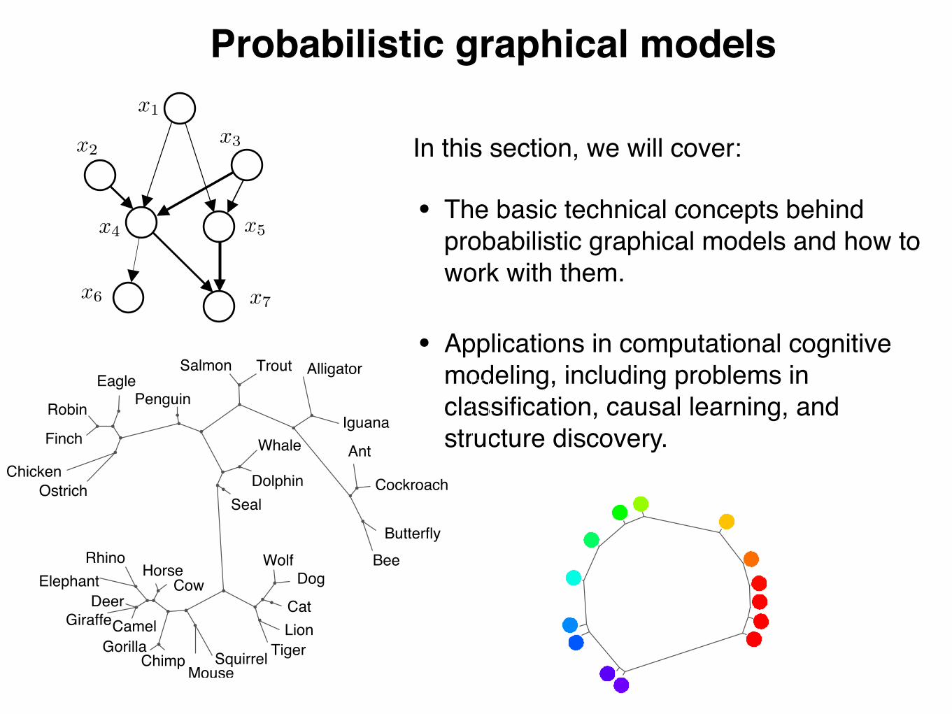
Probabilistic graphical models
• The basic technical concepts behind probabilistic graphical models and how to work with them.
• Applications in computational cognitive modeling, including problems in classification, causal learning, and structure discovery.
In this section, we will cover:
extent to which graphs with many clusters are penalized, and isfixed for all of our experiments. The normalizing constant forP(S!F) depends on the number of structures compatible with agiven form, and ensures that simpler forms are preferred when-
ever possible. For example, any chain Sc is a special case of a grid,but P(Sc!F ! chain) " P(Sc!F ! grid) because there are morepossible grids than chains given a fixed number of entities. Itfollows that P(Sc, F ! chain!D) " P(Sc, F ! grid!D) for any
NewYork
Bombay
Buenos Aires
Moscow
Sao Paulo
Mexico City
Jakarta
Tokyo
Lima
London
Bangkok
SantiagoLos Angeles
Berlin
Madrid
ChicagoVancouverToronto
Sydney
Perth
Anchorage
Cape Town
Nairobi
Vladivostok
Dakar
Kinshasa
Bogota
Honolulu
Wellington
CairoShanghai
Teheran
Irkutsk
Manila
Budapest
GinsburgBrennanScalia
Thomas
O'Connor
Kennedy
WhiteSouter
BreyerMarshallBlackmun Stevens Rehnquist
B
C
ElephantRhino Horse
Cow
CamelGiraffe
ChimpGorilla
MouseSquirrel Tiger
LionCat
DogWolf
SealDolphin
RobinEagle
Chicken
Salmon Trout
Bee
Iguana
Alligator
Butterfly
AntFinch
Penguin
Cockroach
Whale
Ostrich
Deer
E
A
D
Fig. 3. Structures learned from biological features (A), Supreme Court votes (B), judgments of the similarity between pure color wavelengths (C), Euclideandistances between faces represented as pixel vectors (D), and distances between world cities (E). For A–C, the edge lengths represent maximum a posteriori edgelengths under our generative model.
4
3
5
21
WolfowitzRicePowellAshcroftCheneyCard
1
Bush
MyersFeith
Armitage
Libby
DC
Whitman
Rumsfeld
111 321
23
A
P CAB R WL CABRMWRP
WFMR
6
CLCW
A
F
A B
Fig. 4. Structures learned from relational data (Upper) and the raw data organized according to these structures (Lower). (A) Dominance relationships among a troopof sooty mangabeys. The sorted data matrix has most of its entries above the diagonal, indicating that animals tend to dominate only the animals below them in theorder. (B) A hierarchy representing interactions between members of the Bush administration. (C) Social cliques representing friendship relations between prisoners.The sorted matrix has most of its entries along the diagonal, indicating that prisoners tend only to be friends with prisoners in the same cluster. (D) The Kula ringrepresenting armshell trade between New Guinea communities. The relative positions of the communities correspond approximately to their geographic locations.
Kemp and Tenenbaum PNAS ! August 5, 2008 ! vol. 105 ! no. 31 ! 10689CO
MPU
TER
SCIE
NCE
SPS
YCHO
LOG
YSE
ECO
MM
ENTA
RY
x1
x2x3
x4 x5
x6 x7
extent to which graphs with many clusters are penalized, and isfixed for all of our experiments. The normalizing constant forP(S!F) depends on the number of structures compatible with agiven form, and ensures that simpler forms are preferred when-
ever possible. For example, any chain Sc is a special case of a grid,but P(Sc!F ! chain) " P(Sc!F ! grid) because there are morepossible grids than chains given a fixed number of entities. Itfollows that P(Sc, F ! chain!D) " P(Sc, F ! grid!D) for any
NewYork
Bombay
Buenos Aires
Moscow
Sao Paulo
Mexico City
Jakarta
Tokyo
Lima
London
Bangkok
SantiagoLos Angeles
Berlin
Madrid
ChicagoVancouverToronto
Sydney
Perth
Anchorage
Cape Town
Nairobi
Vladivostok
Dakar
Kinshasa
Bogota
Honolulu
Wellington
CairoShanghai
Teheran
Irkutsk
Manila
Budapest
GinsburgBrennanScalia
Thomas
O'Connor
Kennedy
WhiteSouter
BreyerMarshallBlackmun Stevens Rehnquist
B
C
ElephantRhino Horse
Cow
CamelGiraffe
ChimpGorilla
MouseSquirrel Tiger
LionCat
DogWolf
SealDolphin
RobinEagle
Chicken
Salmon Trout
Bee
Iguana
Alligator
Butterfly
AntFinch
Penguin
Cockroach
Whale
Ostrich
Deer
E
A
D
Fig. 3. Structures learned from biological features (A), Supreme Court votes (B), judgments of the similarity between pure color wavelengths (C), Euclideandistances between faces represented as pixel vectors (D), and distances between world cities (E). For A–C, the edge lengths represent maximum a posteriori edgelengths under our generative model.
4
3
5
21
WolfowitzRicePowellAshcroftCheneyCard
1
Bush
MyersFeith
Armitage
Libby
DC
Whitman
Rumsfeld
111 321
23
A
P CAB R WL CABRMWRP
WFMR
6
CLCW
A
F
A B
Fig. 4. Structures learned from relational data (Upper) and the raw data organized according to these structures (Lower). (A) Dominance relationships among a troopof sooty mangabeys. The sorted data matrix has most of its entries above the diagonal, indicating that animals tend to dominate only the animals below them in theorder. (B) A hierarchy representing interactions between members of the Bush administration. (C) Social cliques representing friendship relations between prisoners.The sorted matrix has most of its entries along the diagonal, indicating that prisoners tend only to be friends with prisoners in the same cluster. (D) The Kula ringrepresenting armshell trade between New Guinea communities. The relative positions of the communities correspond approximately to their geographic locations.
Kemp and Tenenbaum PNAS ! August 5, 2008 ! vol. 105 ! no. 31 ! 10689
COM
PUTE
RSC
IEN
CES
PSYC
HOLO
GY
SEE
COM
MEN
TARY

Bayesian networks (“Bayes net”)
• Bayesian network: a directed graph that represents dependencies between random variables, giving a concise specification of a joint probability distribution.
• In a well-constructed network, an arrow indicates that two variables have a path of direct (causal) influence.
• Bayesian networks must be directed, acyclic graphs (DAGs), meaning that they have no cycles.
x1 x2
x3
Factorization of the joint distribution:
edge
node
x1 and x2 are parents of x3
P (x1, x2, x3) = P (x1)P (x2)P (x3|x1, x2)

x1
x2x3
x4 x5
x6 x7
P (x1, . . . , x7) = P (x1)P (x2)P (x3)P (x4|x1, x2, x3)
P (x5|x1, x3)P (x6|x4)P (x7|x4, x5)
Bayesian networks
P (X) =KY
i=1
P (xi|Parents(xi))
General formula for factorizing the joint distribution over a Bayes net:
Slide credit: Christopher Bishop
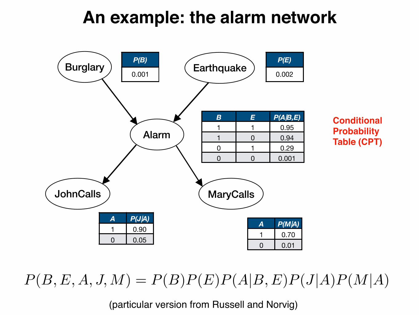
An example: the alarm network
Conditional Probability Table (CPT)
P (B,E,A, J,M) = P (B)P (E)P (A|B,E)P (J |A)P (M |A)
(particular version from Russell and Norvig)
Burglary Earthquake
Alarm
JohnCalls MaryCalls
P(B)
0.001
P(E)
0.002
B E P(A|B,E)1 1 0.951 0 0.940 1 0.290 0 0.001
A P(J|A)1 0.900 0.05
A P(M|A)1 0.700 0.01

P (B,E,A, J,M) = P (B)P (E)P (A|B,E)P (J |A)P (M |A)
Evaluating the joint probability of data
P (B = 0, E = 0, A = 1, J = 1,M = 1)
= P (B = 0)P (E = 0)P (A = 1|B = 0, E = 0)P (J = 1|A = 1)P (M = 1|A = 1)
= 0.999 ⇤ 0.998 ⇤ 0.001 ⇤ 0.9 ⇤ 0.7 = 0.00063
What is the probability that there is no burglary or earthquake, and yet the alarm rings and both John and Mary call?
We use the decomposed joint distribution to evaluate the probability of a setting of all of the variables.
Burglary Earthquake
Alarm
JohnCalls MaryCalls
P(B)
0.001
P(E)
0.002
B E P(A|B,E)1 1 0.951 0 0.940 1 0.290 0 0.001
A P(J|A)1 0.900 0.05
A P(M|A)1 0.700 0.01
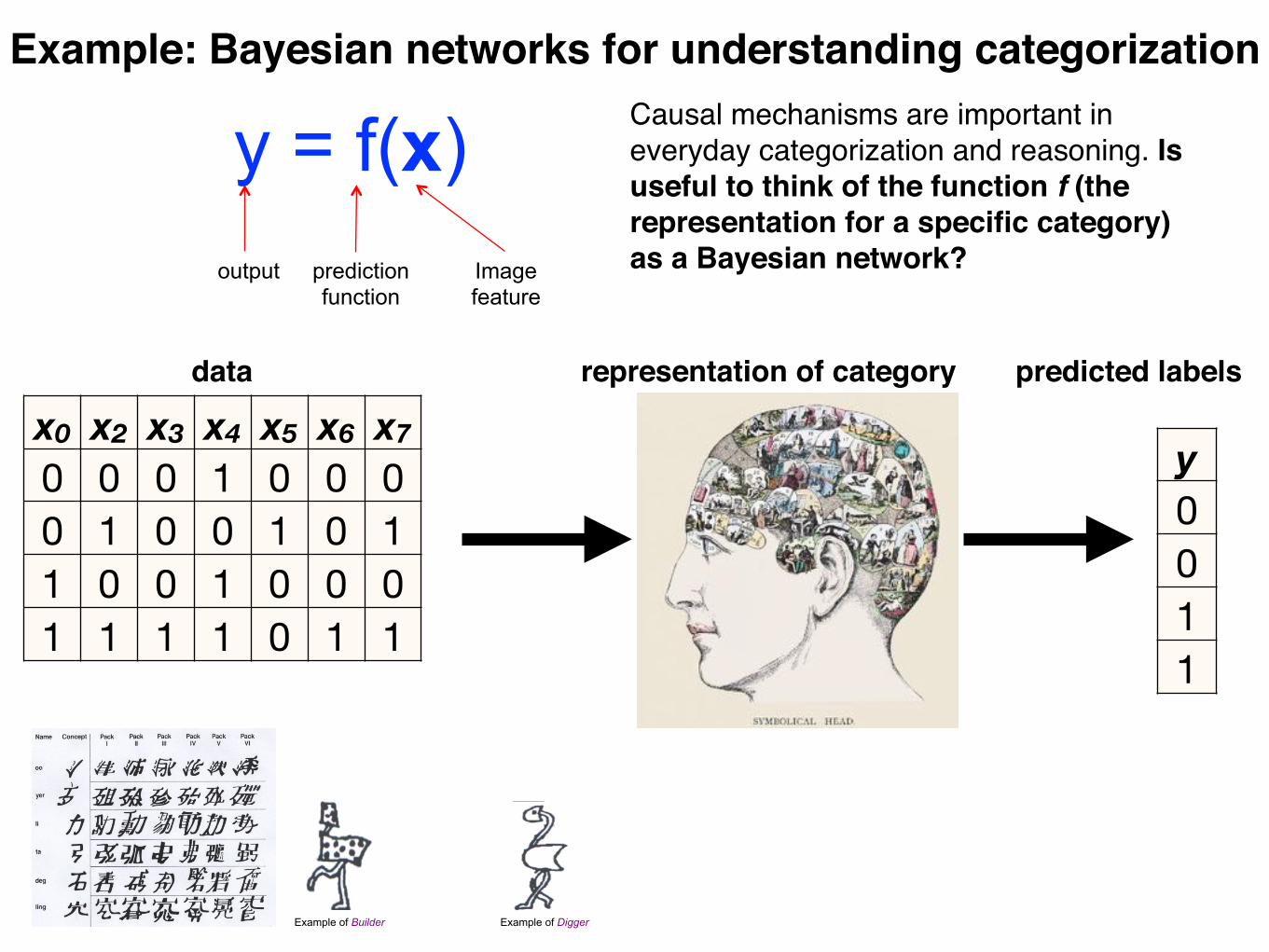
Example: Bayesian networks for understanding categorization
output prediction function
Image feature
y = f(x)
x0 x2 x3 x4 x5 x6 x70 0 0 1 0 0 00 1 0 0 1 0 11 0 0 1 0 0 01 1 1 1 0 1 1
y0011
Example of Builder Example of Digger
data representation of category predicted labels
Causal mechanisms are important in everyday categorization and reasoning. Is useful to think of the function f (the representation for a specific category) as a Bayesian network?
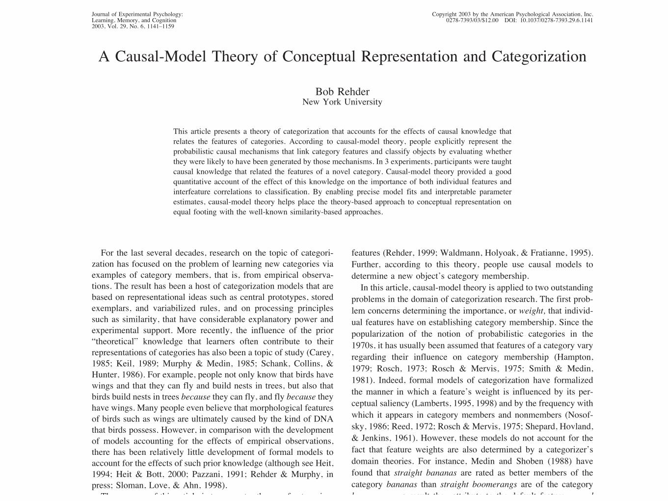
A Causal-Model Theory of Conceptual Representation and Categorization
Bob RehderNew York University
This article presents a theory of categorization that accounts for the effects of causal knowledge thatrelates the features of categories. According to causal-model theory, people explicitly represent theprobabilistic causal mechanisms that link category features and classify objects by evaluating whetherthey were likely to have been generated by those mechanisms. In 3 experiments, participants were taughtcausal knowledge that related the features of a novel category. Causal-model theory provided a goodquantitative account of the effect of this knowledge on the importance of both individual features andinterfeature correlations to classification. By enabling precise model fits and interpretable parameterestimates, causal-model theory helps place the theory-based approach to conceptual representation onequal footing with the well-known similarity-based approaches.
For the last several decades, research on the topic of categori-zation has focused on the problem of learning new categories viaexamples of category members, that is, from empirical observa-tions. The result has been a host of categorization models that arebased on representational ideas such as central prototypes, storedexemplars, and variabilized rules, and on processing principlessuch as similarity, that have considerable explanatory power andexperimental support. More recently, the influence of the prior“theoretical” knowledge that learners often contribute to theirrepresentations of categories has also been a topic of study (Carey,1985; Keil, 1989; Murphy & Medin, 1985; Schank, Collins, &Hunter, 1986). For example, people not only know that birds havewings and that they can fly and build nests in trees, but also thatbirds build nests in trees because they can fly, and fly because theyhave wings. Many people even believe that morphological featuresof birds such as wings are ultimately caused by the kind of DNAthat birds possess. However, in comparison with the developmentof models accounting for the effects of empirical observations,there has been relatively little development of formal models toaccount for the effects of such prior knowledge (although see Heit,1994; Heit & Bott, 2000; Pazzani, 1991; Rehder & Murphy, inpress; Sloman, Love, & Ahn, 1998).The purpose of this article is to present a theory of categoriza-
tion that accounts for the effects of theoretical knowledge, partic-ularly causal knowledge, that interrelates or links the features ofmany categories that people possess. According to causal-modeltheory, people’s knowledge of many categories includes not just arepresentation of a category’s features but also an explicit repre-sentation of the causal mechanisms that people believe link those
features (Rehder, 1999; Waldmann, Holyoak, & Fratianne, 1995).Further, according to this theory, people use causal models todetermine a new object’s category membership.In this article, causal-model theory is applied to two outstanding
problems in the domain of categorization research. The first prob-lem concerns determining the importance, or weight, that individ-ual features have on establishing category membership. Since thepopularization of the notion of probabilistic categories in the1970s, it has usually been assumed that features of a category varyregarding their influence on category membership (Hampton,1979; Rosch, 1973; Rosch & Mervis, 1975; Smith & Medin,1981). Indeed, formal models of categorization have formalizedthe manner in which a feature’s weight is influenced by its per-ceptual saliency (Lamberts, 1995, 1998) and by the frequency withwhich it appears in category members and nonmembers (Nosof-sky, 1986; Reed, 1972; Rosch & Mervis, 1975; Shepard, Hovland,& Jenkins, 1961). However, these models do not account for thefact that feature weights are also determined by a categorizer’sdomain theories. For instance, Medin and Shoben (1988) havefound that straight bananas are rated as better members of thecategory bananas than straight boomerangs are of the categoryboomerangs, a result they attribute to the default feature curvedoccupying a more theoretically central position in the conceptualrepresentation of boomerang as compared with banana (also seeKaplan & Murphy, 2000; Murphy & Allopenna, 1994; Pazzani,1991; Wattenmaker, Dewey, Murphy, & Medin, 1986). Keil(1989) found that second and fourth graders judged that animalswith transformed perceptual features retained their category mem-bership (e.g., a raccoon that is made skunk-like by being dyedblack, painted with a white stripe, and given a “sac of super smellyyucky stuff” is still a raccoon), a result Keil attributed to thechildren’s belief that the theoretically central (albeit hidden) fea-tures of the kind important for category membership had been leftunaltered (also see Gelman &Wellman, 1991; Rips, 1989). Rehderand Hastie (2001) showed that category features involved in manycausal relationships have more influence on category judgmentsthan other features (for related results, see Ahn, 1998; Ahn, Kim,Lassaline, & Dennis, 2000; Sloman et al., 1998).
I thank Patricia Berretty, Seth Chin-Parker, Reid Hastie, Evan Heit,Greg Murphy, Brian Ross, Cindy Sifonis, and two anonymous reviewersfor their comments on earlier versions of this article. Support for thisresearch was provided by Grants SBR-9816458 and SBR 97-20304 fromthe National Science Foundation and Grant R01 MH58362 from theNational Institute of Mental Health.Correspondence concerning this article should be addressed to Bob
Rehder, Department of Psychology, New York University, 6 WashingtonPlace, New York, New York 10003. E-mail: [email protected]
Journal of Experimental Psychology: Copyright 2003 by the American Psychological Association, Inc.Learning, Memory, and Cognition2003, Vol. 29, No. 6, 1141–1159
0278-7393/03/$12.00 DOI: 10.1037/0278-7393.29.6.1141
1141

Four binary featuresF1: High amounts of ACh neurotransmitter. F2: Long-lasting flight response. F3: Accelerated sleep cycle.F4: High body weight.
Artificial categorization task
Task: Learn and make predictions about a new category, e.g., “Lake Victoria Shrimp”
Base rate information: 75% of Lake Victoria Shrimp have each feature, e.g., 75% have feature F4
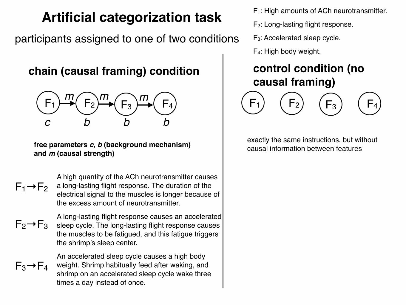
chain (causal framing) condition control condition (no causal framing)
A high quantity of the ACh neurotransmitter causes a long-lasting flight response. The duration of the electrical signal to the muscles is longer because of the excess amount of neurotransmitter.
A long-lasting flight response causes an accelerated sleep cycle. The long-lasting flight response causes the muscles to be fatigued, and this fatigue triggers the shrimp’s sleep center.
An accelerated sleep cycle causes a high body weight. Shrimp habitually feed after waking, and shrimp on an accelerated sleep cycle wake three times a day instead of once.
F1: High amounts of ACh neurotransmitter.
F2: Long-lasting flight response.
F3: Accelerated sleep cycle.
F4: High body weight.
F1→F2
F2→F3
F3→F4
free parameters c, b (background mechanism) and m (causal strength)
exactly the same instructions, but without causal information between features
Artificial categorization taskparticipants assigned to one of two conditions
F1 F2 F3 F4
c b b b
mmm F1 F2 F3 F4
probabilities are greater than 0, reflecting that the joint presence(or the joint absence) of two features directly connected by causalrelationships increased category membership ratings above andbeyond the presence (or absence) of each feature individually. Incomparison, in the control condition the six contrasts were allapproximately 0, indicating that correlations between features hadno influence on category membership ratings in that condition.A two-way ANOVA of these contrasts with condition (chain vs.
control) and contrast (!21, !32, !43, !31, !42, or !41) as factorsconfirmed that the pattern of contrasts differed between the twoconditions as indicated by a significant interaction between con-dition and contrast, F(5, 350) " 4.53, MSE " 0.00551, p # .001.In a separate analysis of the chain condition, the contrasts associ-ated with directly connected feature pairs (!21, !32, !43) weregreater than those associated with indirectly connected pairs (!31,!42, !41), F(1, 35) " 12.0, MSE " 0.00551, p # .001.Theoretical modeling. To demonstrate that the pattern of re-
sults in Experiment 1 is in accordance with the predictions ofcausal-model theory, the chain model of Figure 1B was fit to thecategorization ratings in the chain condition. That is, the values ofparameters c, m, b, and K that minimize the squared difference
between the ratings and the model likelihoods as computed by theequations in Table 3 was determined for each of the 36 chainparticipants. The parameter values averaged over participants arepresented in Table 5. The table also presents for each model thesquared error averaged over participants (Avg. SSE), and theroot-mean-square deviation (RMSD) averaged over participants(Avg. RMSD), where RMSD " SQRT(SSE/(N $ P)), N is thenumber of observations modeled (16), and P is the total number ofparameters in the model (4).According to causal-model theory, parameter m represents the
probability that a causal mechanism between two category featureswill operate (i.e., will bring about the presence of its effect) whenthe cause feature is present. Table 5 indicates an estimate ofparameter m of .120. That is, the fit of the chain model indicatesthat participants generated categorization ratings in a manner con-sistent with a belief in the presence of probabilistic causal mech-anisms arranged in a causal chain. To illustrate the chain model’ssensitivity to correlations between features directly linked bycausal mechanisms, its predicted ratings for exemplars 0000, 0101,1010, and 1111 are presented in Figure 3, superimposed on theempirical ratings. The chain model correctly predicted both thelower categorization ratings for those exemplars that possessedmany violations of causal knowledge (0101 and 1010) and thehigher categorization ratings for those exemplars that confirmedcausal knowledge (1111).To demonstrate the chain model’s fit directly in terms of feature
probabilities and correlations, I computed the probabilities andcorrelations implied by the chain model fit. That is, for eachparticipant the chain model predicts certain likelihoods for eachexemplar, and feature probabilities and interfeature contrasts canbe computed from these likelihoods. These probabilities and con-trasts were then averaged over participants and these averages arepresented in Figure 3B, superimposed on the empirical data. Fig-ure 3B confirms that the chain model was able to account for boththe weights associated with the individual features and the sensi-tivity to correlated features displayed by participants. Indeed, thechain model’s predicted ratings accounted for 97% of the variancein the average ratings.
Table 5Parameter Estimates and Measures of Fit of the Chain CausalModel to the Chain Conditions of Experiments 1–3
Parameters andmeasures
Experiment
1 2 3
M SE M SE M SE
c .598 .017 .525 .016m .120 .026 .402 .053 .266 .044b .521 .014 .384 .026 .464 .031K 815 25.3 642 42.1 403 20.7Average SSE 2157 2309 893Average RMSD 12.4 12.4 11.7R2 .97 .93 .97
Note. Average SSE " sum of squared error averaged over participants;Average RMSD " root-mean-square deviation averaged over participants.Parameter c was not estimated in Experiment 3.
Figure 3. Results from the chain and control conditions of Experiment 1.A: Categorization ratings for selected exemplars. B: Derived feature prob-abilities and interfeature correlations. Predictions of the chain model areshown in each panel.
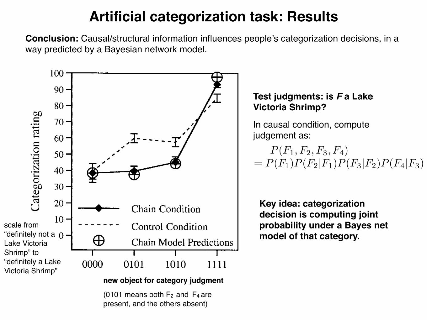
1148 REHDERArtificial categorization task: Results
scale from “definitely not a Lake Victoria Shrimp” to “definitely a Lake Victoria Shrimp”
Conclusion: Causal/structural information influences people’s categorization decisions, in a way predicted by a Bayesian network model.
new object for category judgment
(0101 means both F2 and F4 are present, and the others absent)
P (F1, F2, F3, F4)= P (F1)P (F2|F1)P (F3|F2)P (F4|F3)
Test judgments: is F a Lake Victoria Shrimp?
In causal condition, compute judgement as:
Key idea: categorization decision is computing joint probability under a Bayes net model of that category.

F1
F2
F3
F1
F2
F3
F2F4F4
Further work from Rehder and colleagues have studied categories with these alternative Bayes net structures…(e.g., Rehder and Hastie, 2001)
Causal structure matters in categorization judgments
F1 F2 F3 F4
c b b b
mmm
F1 F2 F3 F4
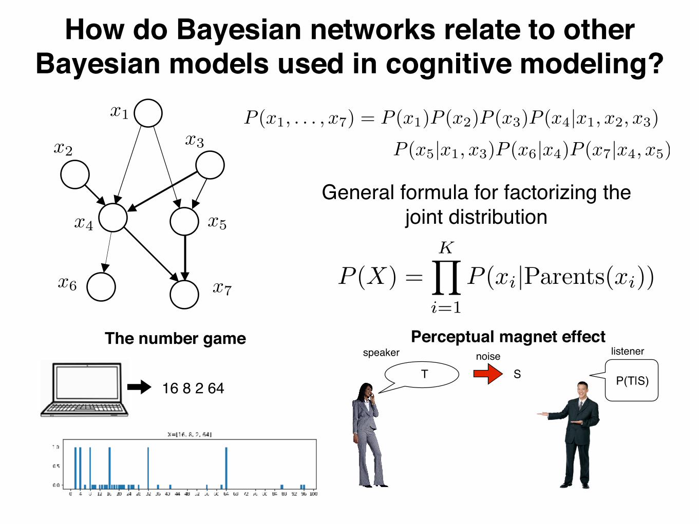
x1
x2x3
x4 x5
x6 x7
P (x1, . . . , x7) = P (x1)P (x2)P (x3)P (x4|x1, x2, x3)
P (x5|x1, x3)P (x6|x4)P (x7|x4, x5)
P (X) =KY
i=1
P (xi|Parents(xi))
General formula for factorizing the joint distribution
How do Bayesian networks relate to other Bayesian models used in cognitive modeling?
16 8 2 64
The number game
T Snoise
P(T|S)
The speaker makes an intended sound production T.Noise in the air perturbs T into S.The listener calculates the posterior P(T|S)
P (T |S) =P (S|T )P (T )
P (S)
noisespeech sound from
speakerperception
Bayesian model of speech perceptionspeaker listener
Perceptual magnet effect
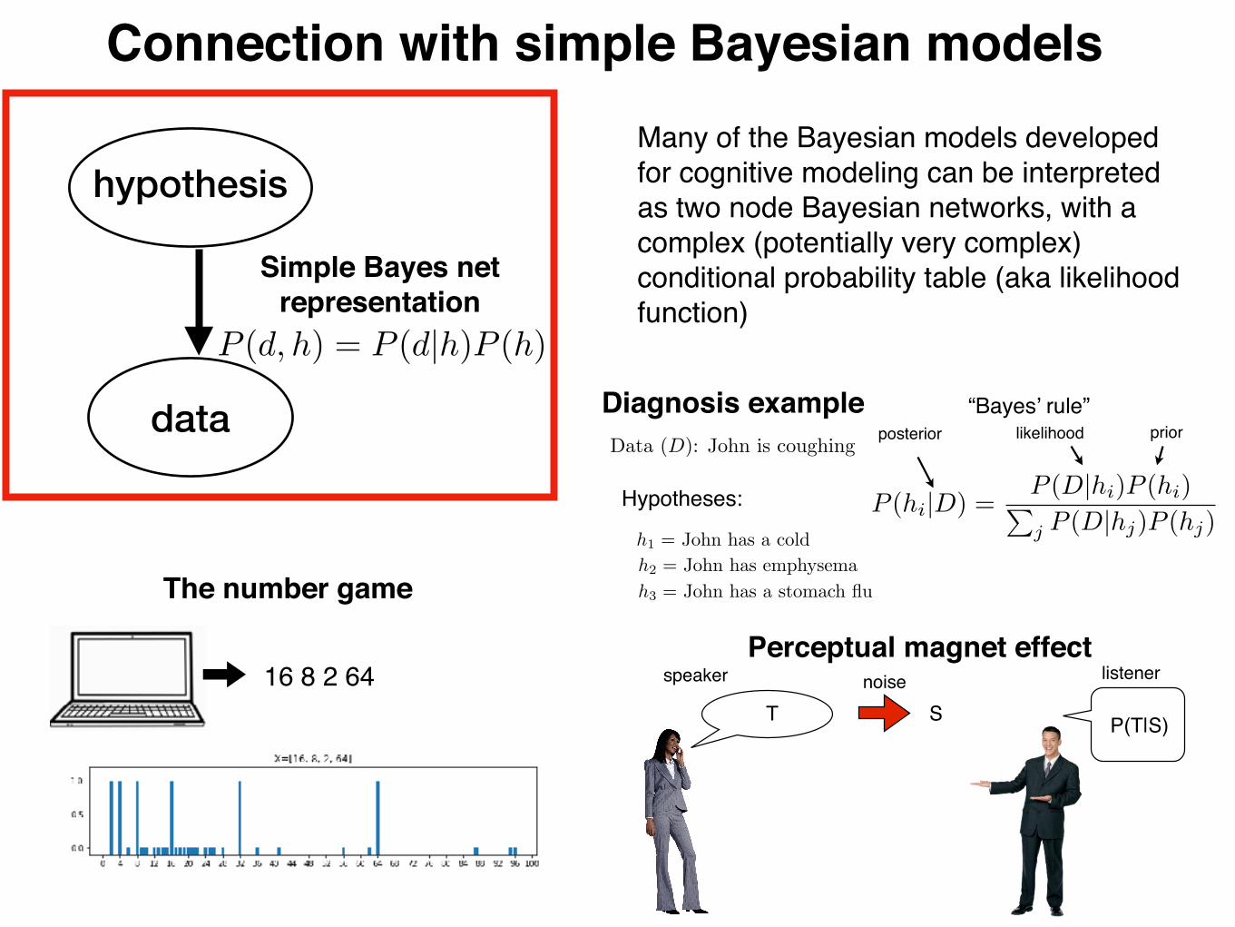
Data (D): John is coughing
h1 = John has a coldh2 = John has emphysemah3 = John has a stomach flu
Hypotheses:
Connection with simple Bayesian models
16 8 2 64
The number game
T Snoise
P(T|S)
The speaker makes an intended sound production T.Noise in the air perturbs T into S.The listener calculates the posterior P(T|S)
P (T |S) =P (S|T )P (T )
P (S)
noisespeech sound from
speakerperception
Bayesian model of speech perceptionspeaker listener
Diagnosis example
hypothesis
data
Simple Bayes net representation Bayesian inference for evaluating
hypotheses in light of data
Data (D): John is coughing
h1 = John has a coldh2 = John has emphysemah3 = John has a stomach flu
We want to calculate the posterior probabilities: P (h1|D), P (h2|D), and P (h3|D)
Hypotheses:
Which hypotheses should we believe, and with what certainty?
priorlikelihoodposterior
P (hi|D) =P (D|hi)P (hi)Pj P (D|hj)P (hj)
“Bayes’ rule”
Example from Josh Tenenbaum
Many of the Bayesian models developed for cognitive modeling can be interpreted as two node Bayesian networks, with a complex (potentially very complex) conditional probability table (aka likelihood function)
Perceptual magnet effect
P (d, h) = P (d|h)P (h)
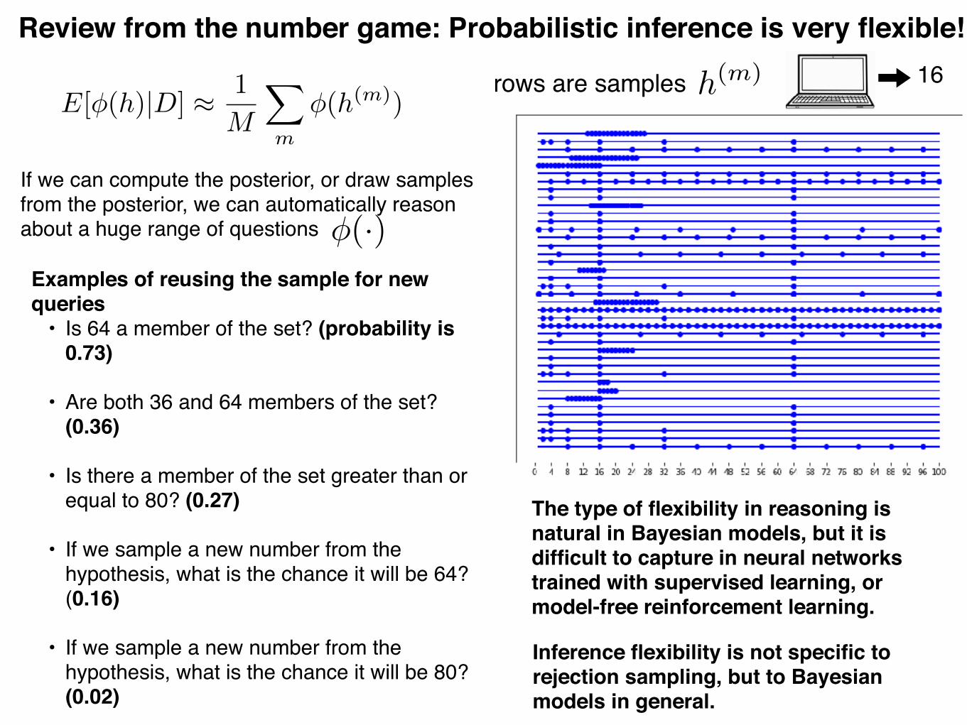
Review from the number game: Probabilistic inference is very flexible!
E[�(h)|D] ⇡ 1
M
X
m
�(h(m))
If we can compute the posterior, or draw samples from the posterior, we can automatically reason about a huge range of questions
rows are samples h(m)
Examples of reusing the sample for new queries
• Is 64 a member of the set? (probability is 0.73)
• Are both 36 and 64 members of the set? (0.36)
• Is there a member of the set greater than or equal to 80? (0.27)
• If we sample a new number from the hypothesis, what is the chance it will be 64? (0.16)
• If we sample a new number from the hypothesis, what is the chance it will be 80? (0.02)
�(·)
The type of flexibility in reasoning is natural in Bayesian models, but it is difficult to capture in neural networks trained with supervised learning, or model-free reinforcement learning.
Inference flexibility is not specific to rejection sampling, but to Bayesian models in general.
16
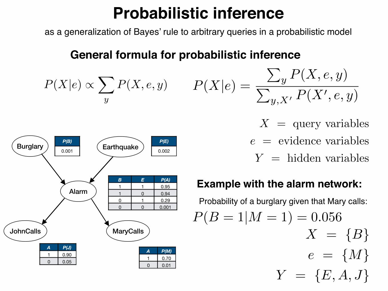
Probabilistic inferenceas a generalization of Bayes’ rule to arbitrary queries in a probabilistic model
General formula for probabilistic inference
P (X|e) /X
y
P (X, e, y)
X = query variables
e = evidence variables
Y = hidden variablesBurglary Earthquake
Alarm
JohnCalls MaryCalls
P(B)
0.001
P(E)
0.002
B E P(A)1 1 0.951 0 0.940 1 0.290 0 0.001
A P(J)1 0.900 0.05
A P(M)1 0.700 0.01
Example with the alarm network:
X = {B}e = {M}
Y = {E,A, J}
Probability of a burglary given that Mary calls:
P (X|e) =P
y P (X, e, y)P
y,X0 P (X 0, e, y)
P (B = 1|M = 1) = 0.056
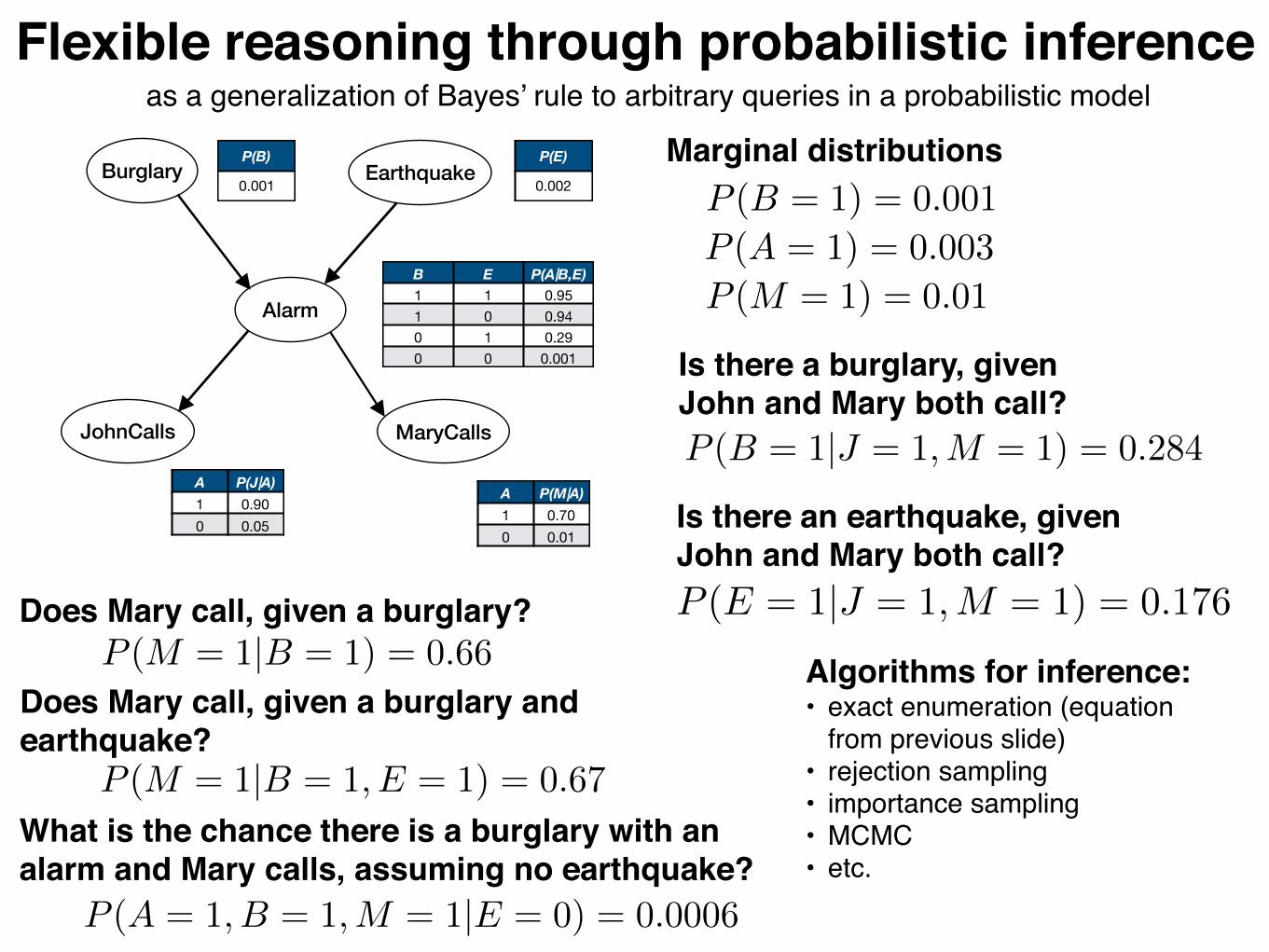
Flexible reasoning through probabilistic inferenceas a generalization of Bayes’ rule to arbitrary queries in a probabilistic model
P (M = 1) = 0.01P (A = 1) = 0.003P (B = 1) = 0.001
Marginal distributions
P (B = 1|J = 1,M = 1) = 0.284
Is there a burglary, given John and Mary both call?
Is there an earthquake, given John and Mary both call?P (E = 1|J = 1,M = 1) = 0.176
P (M = 1|B = 1) = 0.66Does Mary call, given a burglary?
P (M = 1|B = 1, E = 1) = 0.67
Does Mary call, given a burglary and earthquake?
P (A = 1, B = 1,M = 1|E = 0) = 0.0006
What is the chance there is a burglary with an alarm and Mary calls, assuming no earthquake?
Algorithms for inference:• exact enumeration (equation
from previous slide)• rejection sampling• importance sampling• MCMC• etc.
Burglary Earthquake
Alarm
JohnCalls MaryCalls
P(B)
0.001
P(E)
0.002
B E P(A|B,E)1 1 0.951 0 0.940 1 0.290 0 0.001
A P(J|A)1 0.900 0.05
A P(M|A)1 0.700 0.01
Burglary Earthquake
Alarm
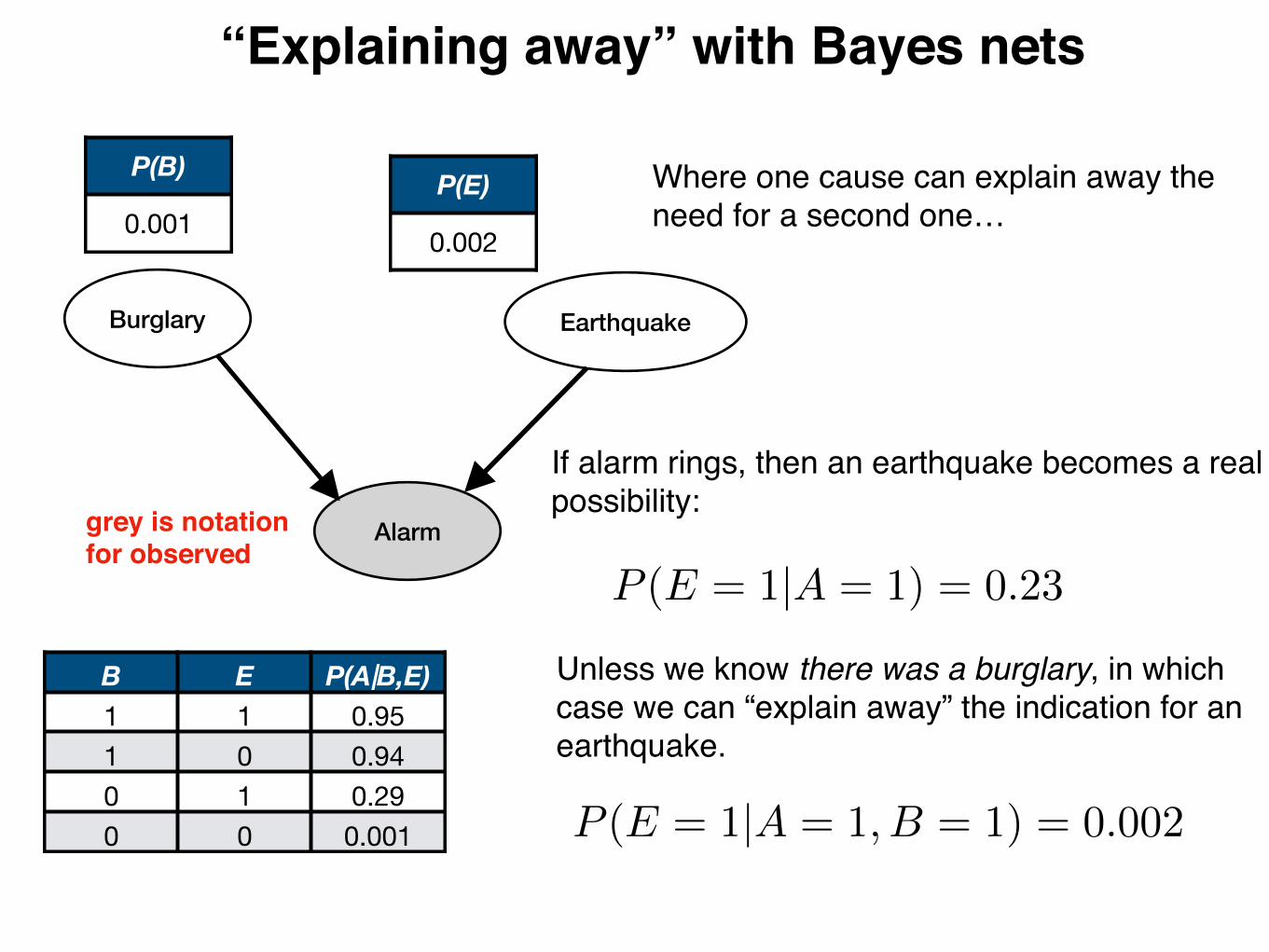
“Explaining away” with Bayes nets
grey is notation for observed
P(B)
0.001P(E)
0.002
B E P(A|B,E)1 1 0.951 0 0.940 1 0.290 0 0.001
P (E = 1|A = 1) = 0.23
P (E = 1|A = 1, B = 1) = 0.002
If alarm rings, then an earthquake becomes a real possibility:
Unless we know there was a burglary, in which case we can “explain away” the indication for an earthquake.
Where one cause can explain away the need for a second one…
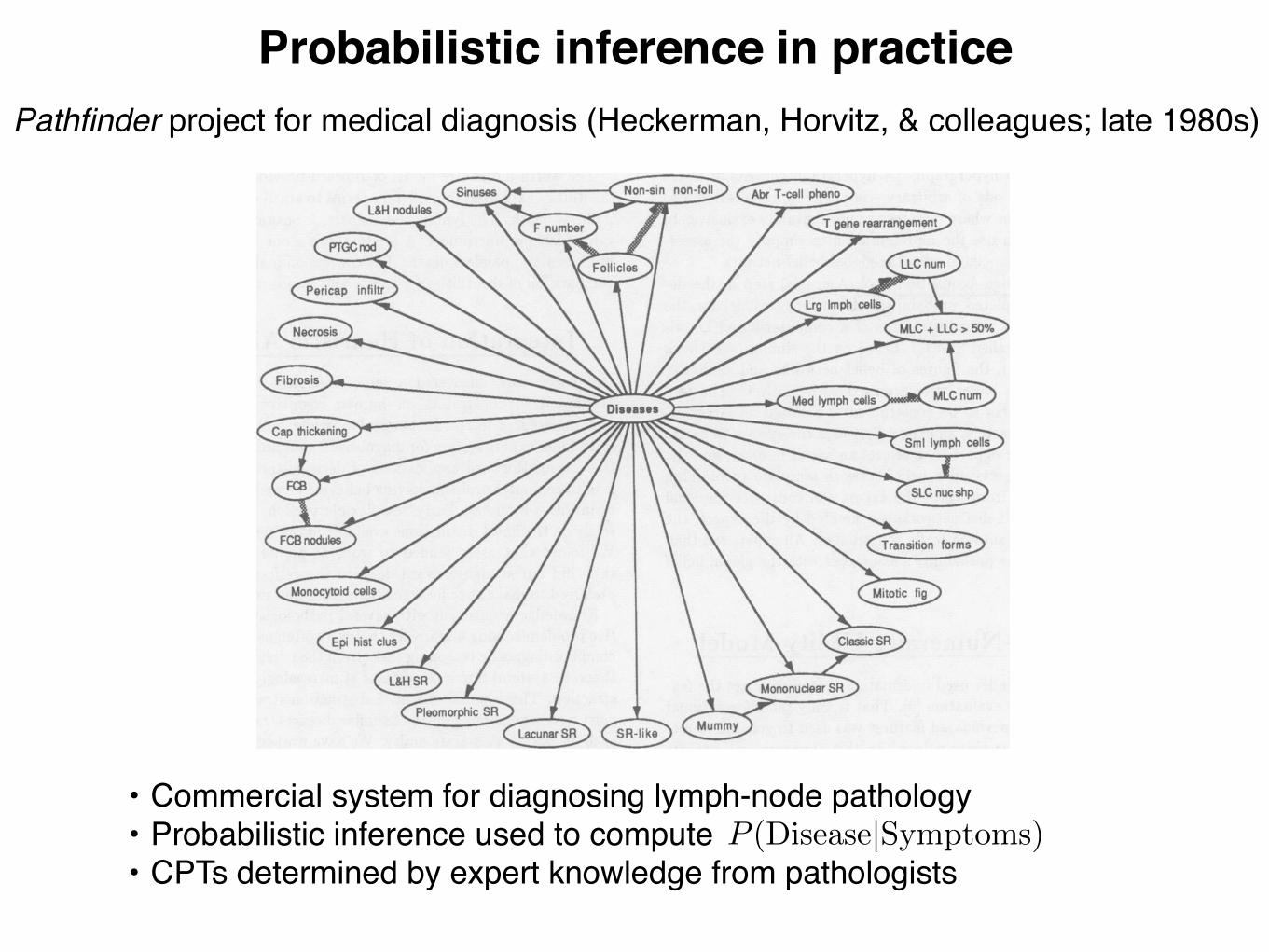
Probabilistic inference in practice
Figure 1: A portion of the Pathfinder belief network. The arcs from the disease node (center) to the features represents the influence of the diseasestate on the appearance of the features. The arcs among the features indicates probabilistic dependency among features. The wider arcs capturethe concept of irrelevancy.
Figure 2: A portion of the similarity graph for Pathfinder. (HD =Hodgkin's disease; NSHD = nodular-sclerosing Hodgkin's disease.)
Figure 3: The local belief network that captures the problem ofdifferentiating mixed-cellularity Hodgkin's disease from interfollicularHodgkin's disease. (F number = follicles number; Non-sin non-foll =nonsinus, nonfollicular areas.)
similarity network for lymph-node disease, was shown in Figure 1. Ithas been demonstrated that, provided the similarity network is com-pletely connected and several other technical conditions are met, theglobal belief network constructed from a similarity network is a validbelief network for the entire domain [5]. Thus, the similarity-networkrepresentation greatly facilitates the construction of large belief net-works. A similarity network allows an expert to decompose the task ofbuilding a large belief network into modular and relatively small sub-tasks. Using a similarity network, an expert can focus his attention onsmall dependency problems for actual clinical dilemmas. In the case oflymph-node pathology, the expert could not construct the global beliefnetwork without the aid of the similarity-network representation.
Several important features of the similarity-network representationare discussed in [5]. For example, similarity networks can be extendedto include local belief networks for sets of hypotheses that contain twoor more elements. Essentially, we need only to replace the similarity
205
----
._Ijixed callularitij HD vo lnterfollicular ___.
Pathfinder project for medical diagnosis (Heckerman, Horvitz, & colleagues; late 1980s)
• Commercial system for diagnosing lymph-node pathology• Probabilistic inference used to compute• CPTs determined by expert knowledge from pathologists
P (Disease|Symptoms)
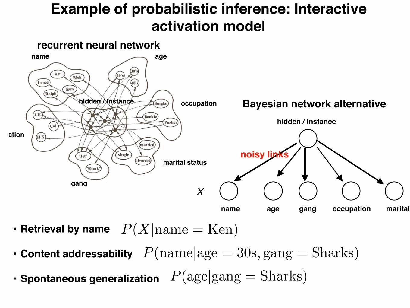
Example of probabilistic inference: Interactive activation model
Interactive activation model
name age
occupation
marital status
gang
education
hidden / instance
(McClelland, 1981)
• Each item is a unit with mutually excitatory connections to its properties• Properties are organized into pools of mutually inhibitory units (e.g., since a
person can’t be both in their 20’s and in their 30’s)recurrent neural network
name age occupation maritalgang
hidden / instance
Bayesian network alternative
noisy links
• Retrieval by name
• Content addressability
• Spontaneous generalization
P (X|name = Ken)
P (name|age = 30s, gang = Sharks)
P (age|gang = Sharks)
X

Conditional independence
x1 is independent of x2 given x3
P (x1|x2, x3) = P (x1|x3)
P (x1, x2|x3) = P (x1|x2, x3)P (x2|x3)
= P (x1|x3)P (x2|x3)
Equivalently
x1 ?? x2 | x3
Written as
(product rule)
Slide credit: Christopher Bishop
Alarm
JohnCalls MaryCalls
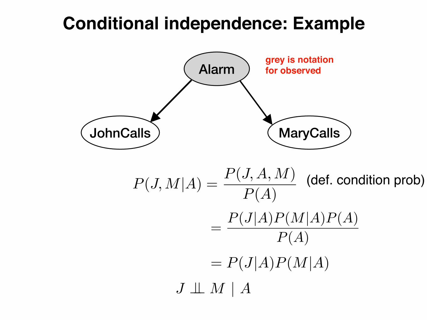
Conditional independence: Example
P (J,M |A) =P (J,A,M)
P (A)
= P (J |A)P (M |A)
J ?? M | A
grey is notation for observed
(def. condition prob)
=P (J |A)P (M |A)P (A)
P (A)
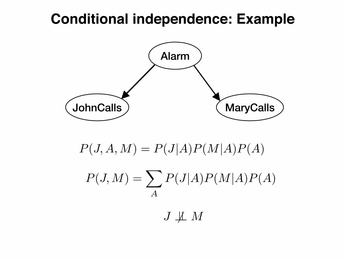
Alarm
JohnCalls MaryCalls
Conditional independence: Example
P (J,A,M) = P (J |A)P (M |A)P (A)
P (J,M) =X
A
P (J |A)P (M |A)P (A)
J 6?? M
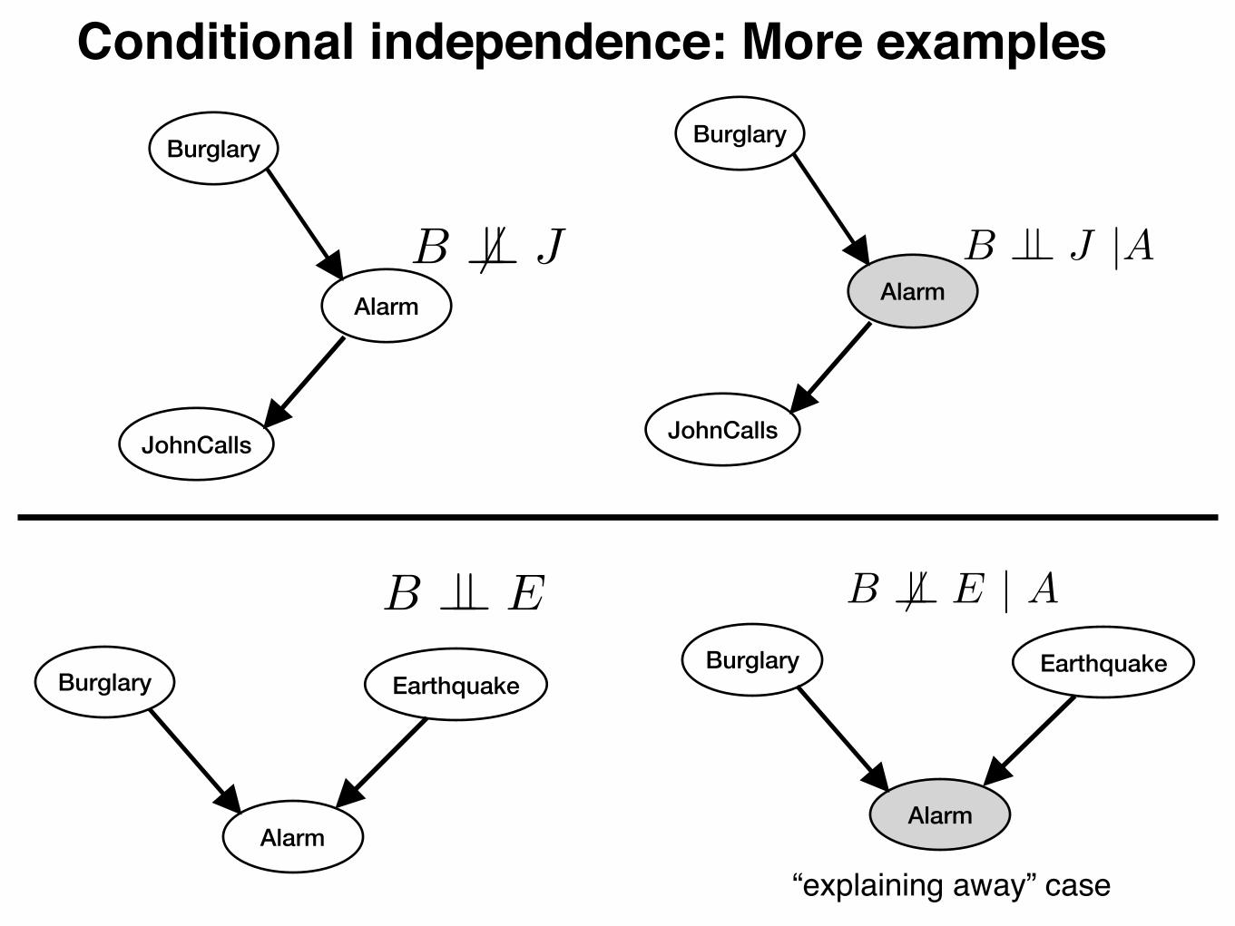
Conditional independence: More examples
Burglary
Alarm
JohnCalls
Burglary
Alarm
JohnCalls
B 6?? J B ?? J |A
Burglary Earthquake
Alarm
Burglary Earthquake
Alarm
B ?? E B 6?? E | A
“explaining away” case
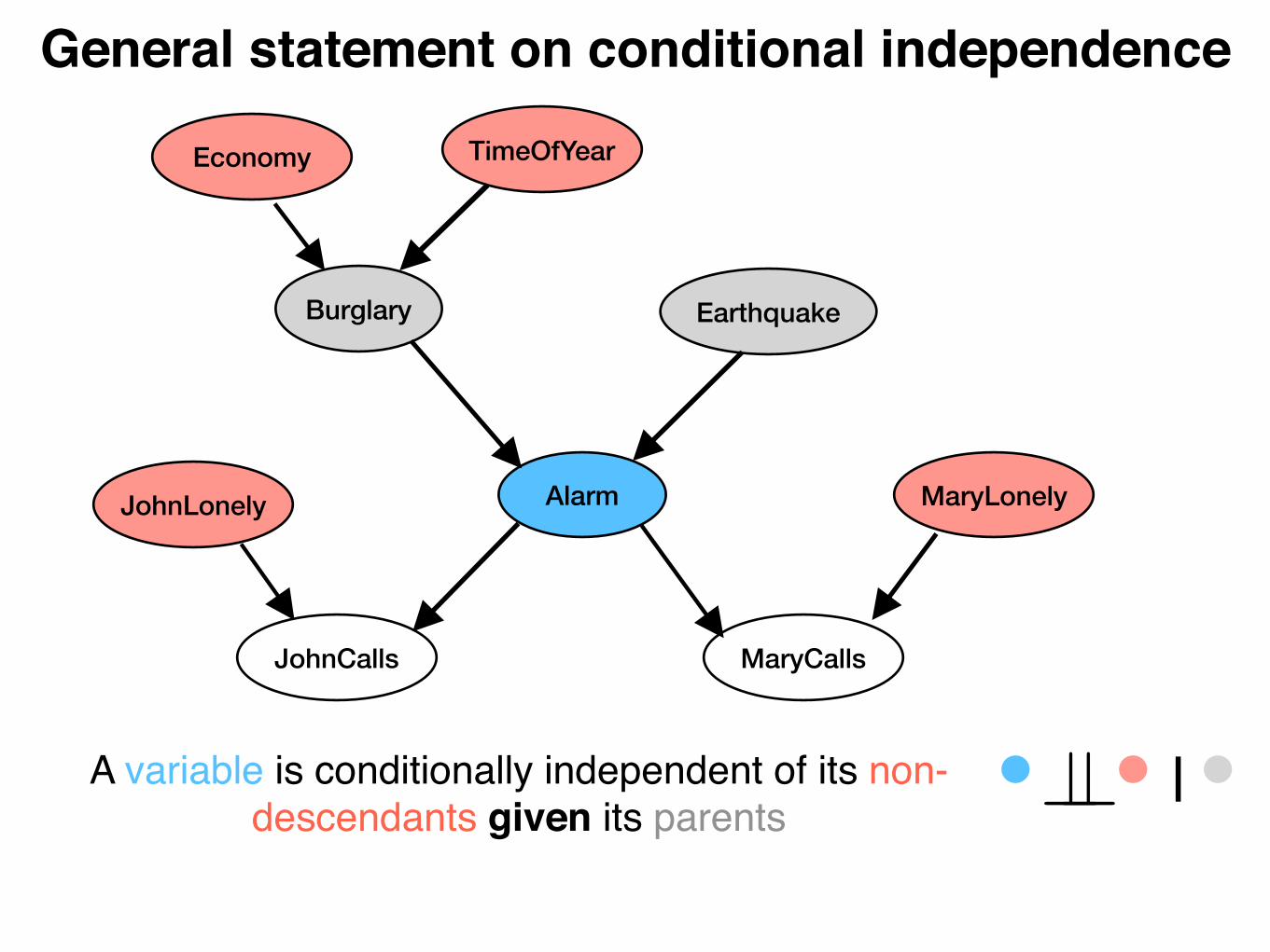
Burglary Earthquake
Alarm
JohnCalls MaryCalls
JohnLonely MaryLonely
Economy TimeOfYear
General statement on conditional independence
A variable is conditionally independent of its non-descendants given its parents ?? |
Burglary Earthquake
Alarm
JohnCalls MaryCalls
JohnLonely MaryLonely
Economy TimeOfYear
General statement on conditional independence
A variable is conditionally independent of its non-descendants given its parents ??
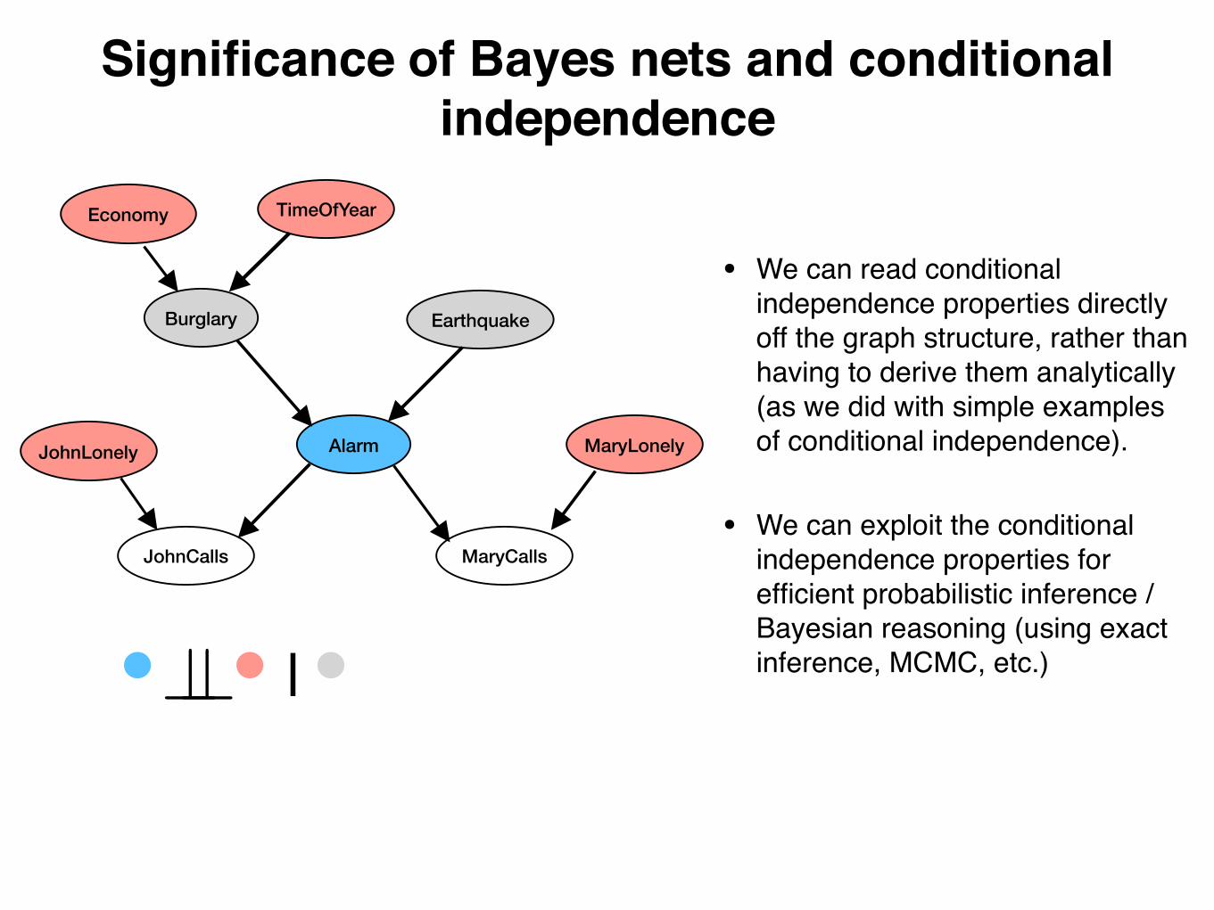
Significance of Bayes nets and conditional independence
?? |
• We can read conditional independence properties directly off the graph structure, rather than having to derive them analytically (as we did with simple examples of conditional independence).
• We can exploit the conditional independence properties for efficient probabilistic inference / Bayesian reasoning (using exact inference, MCMC, etc.)

Learning Bayesian networks: Parameter learning
P (B,E,A, J,M) = P (B)P (E)P (A|B,E)P (J |A)P (M |A)
✓ : parameters (numbers in CPTs)
S : graph structure
D : data set
argmax✓
X
i
logP (D(i)|✓;S)
B E A J M1 0 1 0 10 0 0 0 00 0 0 0 1
example empirical data set D
more rows like this….
D(1)
D(2)
D(N)…
maximum likelihood parameter learning:
straightforward solution: we can fit CPTs independently, and each CPT is very intuitive (simply count the relevant occurrences of a variable given its parents)
Known structure (e.g., consulting experts, prior knowledge), but unknown parameters
Burglary Earthquake
Alarm
JohnCalls MaryCalls
P(B)
0.001
P(E)
0.002
B E P(A|B,E)1 1 0.951 0 0.940 1 0.290 0 0.001
A P(J|A)1 0.900 0.05
A P(M|A)1 0.700 0.01
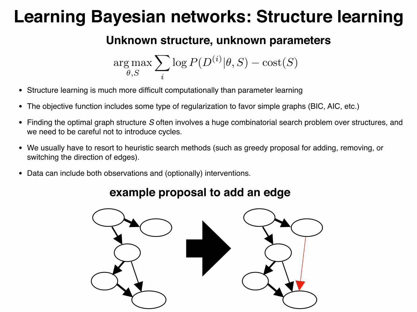
Learning Bayesian networks: Structure learningUnknown structure, unknown parameters
• Structure learning is much more difficult computationally than parameter learning
• The objective function includes some type of regularization to favor simple graphs (BIC, AIC, etc.)
• Finding the optimal graph structure S often involves a huge combinatorial search problem over structures, and we need to be careful not to introduce cycles.
• We usually have to resort to heuristic search methods (such as greedy proposal for adding, removing, or switching the direction of edges).
• Data can include both observations and (optionally) interventions.
argmax✓,S
X
i
logP (D(i)|✓, S)� cost(S)
example proposal to add an edge
Burglary
Earthquake
Alarm
JohnCallsMaryCalls
Burglary
Earthquake
Alarm
JohnCalls
MaryCalls
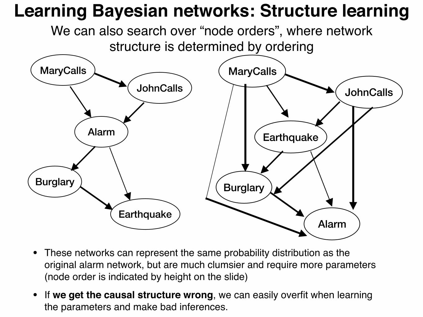
We can also search over “node orders”, where network structure is determined by ordering
• These networks can represent the same probability distribution as the original alarm network, but are much clumsier and require more parameters (node order is indicated by height on the slide)
• If we get the causal structure wrong, we can easily overfit when learning the parameters and make bad inferences.
Learning Bayesian networks: Structure learning
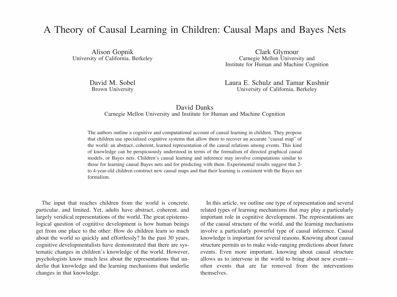
A Theory of Causal Learning in Children: Causal Maps and Bayes Nets
Alison GopnikUniversity of California, Berkeley
Clark GlymourCarnegie Mellon University and
Institute for Human and Machine Cognition
David M. SobelBrown University
Laura E. Schulz and Tamar KushnirUniversity of California, Berkeley
David DanksCarnegie Mellon University and Institute for Human and Machine Cognition
The authors outline a cognitive and computational account of causal learning in children. They proposethat children use specialized cognitive systems that allow them to recover an accurate “causal map” ofthe world: an abstract, coherent, learned representation of the causal relations among events. This kindof knowledge can be perspicuously understood in terms of the formalism of directed graphical causalmodels, or Bayes nets. Children’s causal learning and inference may involve computations similar tothose for learning causal Bayes nets and for predicting with them. Experimental results suggest that 2-to 4-year-old children construct new causal maps and that their learning is consistent with the Bayes netformalism.
The input that reaches children from the world is concrete,particular, and limited. Yet, adults have abstract, coherent, andlargely veridical representations of the world. The great epistemo-logical question of cognitive development is how human beingsget from one place to the other: How do children learn so muchabout the world so quickly and effortlessly? In the past 30 years,cognitive developmentalists have demonstrated that there are sys-tematic changes in children’s knowledge of the world. However,psychologists know much less about the representations that un-derlie that knowledge and the learning mechanisms that underliechanges in that knowledge.
In this article, we outline one type of representation and severalrelated types of learning mechanisms that may play a particularlyimportant role in cognitive development. The representations areof the causal structure of the world, and the learning mechanismsinvolve a particularly powerful type of causal inference. Causalknowledge is important for several reasons. Knowing about causalstructure permits us to make wide-ranging predictions about futureevents. Even more important, knowing about causal structureallows us to intervene in the world to bring about new events—often events that are far removed from the interventionsthemselves.
Alison Gopnik, Laura E. Schulz, and Tamar Kushnir, Department ofPsychology, University of California, Berkeley; Clark Glymour and DavidDanks, Department of Philosophy, Carnegie Mellon University, and Insti-tute for Human and Machine Cognition, Pensacola, Florida; David M.Sobel, Department of Cognitive and Linguistic Science, Brown University.Earlier versions and portions of this article were presented at the meet-
ings of the International Congress on Logic, Methodology, and Philosophyof Science, Krakow, Poland, August 1999; the Rutgers Conference on theCognitive Basis of Science, New Brunswick, NJ, September 1999; theEuropean Society for Philosophy and Psychology meeting, Freiburg, Ger-many, August 2001; the Society for Philosophy and Psychology meeting,Edmonton, Alberta, Canada, June 2002; the Society for Research in ChildDevelopment meeting, Minneapolis, MN, April 2001; and the NeuralInformation Processing Systems meeting, Whistler, British Columbia,Canada, December 2001; and in seminars at the University of Chicago, theCalifornia Institute of Technology, Stanford University, the University ofSanta Cruz, the Santa Fe Institute, and in the Cognitive Science Programand Department of Statistics at the University of California, Berkeley.This research was supported in part by grants from the University of
California, Berkeley, and the Institute of Human Development; by NationalScience Foundation Grant DLS0132487 to Alison Gopnik; by NationalScience Foundation and National Aeronautics and Space Administration
Grants NCC2-1377 and NCC2-1399 to Clark Glymour; by National Insti-tute of Health Awards F31MH12047 to David M. Sobel andF31MH66538-01A1 to Tamar Kushnir; by a National Science Foundationfellowship to Laura E. Schulz; and by McDonnell Foundation support toDavid Danks.Conversations with Steve Palmer, Lucy Jacobs, Andrew Meltzoff, Josh
Tenenbaum, Thierry Nazzi, John Campbell, Peter Godfrey-Smith, HenryWellman, Peter Spirtes, John Watson, Daniel Povinelli, Stuart Russell, andthe Bayes net reading group all played an important role in shaping theseideas, and we are grateful. Jitendra Malik and Marty Banks providedhelpful insights and examples from vision science. Patricia Cheng madeextremely helpful and thorough comments on several drafts of this article.Susan Carey also was very helpful in the revision process. We are alsograteful to Christine Schaeffer and Beverly Slome for help in conductingthe experiments and to the participants in our studies and their parents andteachers.Correspondence concerning this article should be addressed to Alison
Gopnik, who is at the Center for Advanced Study in the BehavioralSciences, 75 Alta Road, Stanford, CA 94305-8090, through June 1, 2004.After June 1, 2004, correspondence should be addressed to Alison Gopnik,Department of Psychology, University of California, Berkeley, CA 94720.E-mail: [email protected]
Psychological Review Copyright 2004 by the American Psychological Association, Inc.2004, Vol. 111, No. 1, 3–32 0033-295X/04/$12.00 DOI: 10.1037/0033-295X.111.1.3
3
The results of these experiments rule out many possible hypoth-eses about children’s causal learning. Because children did notactivate the detector themselves, they could not have solved thesetasks through operant conditioning or through trial-and-error learn-ing. The blickets and nonblickets were perceptually indistinguish-able, and both blocks were in contact with the detector, so childrencould not have solved the tasks through their substantive priorknowledge about everyday physics.The “make it stop” condition in this experiment also showed
that children’s inferences went beyond classical conditioning, sim-ple association, or simple imitative learning. Children not onlyassociated the word and the effect, they combined their priorcausal knowledge and the new causal knowledge they inferredfrom the dependencies to create a brand-new intervention that theyhad never witnessed before. As we mentioned above, this kind ofnovel intervention is the hallmark of a causal map. It is interestingthat there is, to our knowledge, no equivalent of this result in thevast animal conditioning literature, although such an experimentwould be easy to design. Would Pavlov’s dogs, for example,intervene to silence a bell that led to shock, if they had simplyexperienced an association between the bell and the shock but hadnever intervened in this way before?In all these respects, children seemed to have learned a new
causal map. Moreover, this experiment showed that children werenot using simple frequencies to determine the causal structure ofthis map but were using more complex patterns of conditionaldependence. However, this experiment was consistent with all fourlearning models we described above, including the causal inter-pretation of the RW model.
Inference from indirect evidence: Backward blocking. In thenext study we wanted to see whether children’s reasoning wouldextend to even more complex types of conditional dependence and,in particular, if children would reason in ways that went beyondcausal RW. There are a number of experimental results that argueagainst the RW model for adult human causal learning. One suchphenomenon is “backward blocking” (Shanks, 1985; Shanks &Dickinson, 1987; Wasserman & Berglan, 1998). In backwardblocking, learners decide whether an object causes an effect byusing information from trials in which that object never appears.Sobel and colleagues (Sobel, Tenenbaum, & Gopnik, in press)
have demonstrated backward blocking empirically in young chil-dren. In one experiment (Sobel et al., in press, Experiment 2), 3-and 4-year-olds were introduced to the blicket detector in the samemanner as in the Gopnik et al. (2001) experiments. They were toldthat some blocks were blickets and that blickets make the machinego. In a pretest, children saw that some blocks, but not others,made the machine go, and the active objects were labeled asblickets. Then children were shown two new blocks (A and B).In one condition, the control, inference condition, A and B were
placed on the detector together twice, and the detector respondedboth times. Then children observed that Object A did not activatethe detector by itself. In the other condition, the backward blockingcondition, children saw that two new blocks, A and B, activatedthe detector together twice. Then they observed that Block A didactivate the detector by itself. In both conditions, children werethen asked whether each block was a blicket and were asked tomake the machine go (see Figure 13).
Figure 12. Procedure used in Gopnik et al. (2001, Experiment 3).
22 GOPNIK ET AL.
A B
D
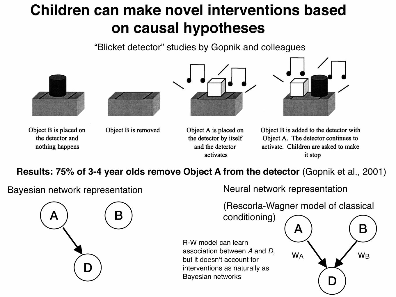
Children can make novel interventions based on causal hypotheses
“Blicket detector” studies by Gopnik and colleagues
Bayesian network representation Neural network representation
(Rescorla-Wagner model of classical conditioning)
A B
D
wA wB
R-W model can learn association between A and D, but it doesn’t account for interventions as naturally as Bayesian networks
Results: 75% of 3-4 year olds remove Object A from the detector (Gopnik et al., 2001)
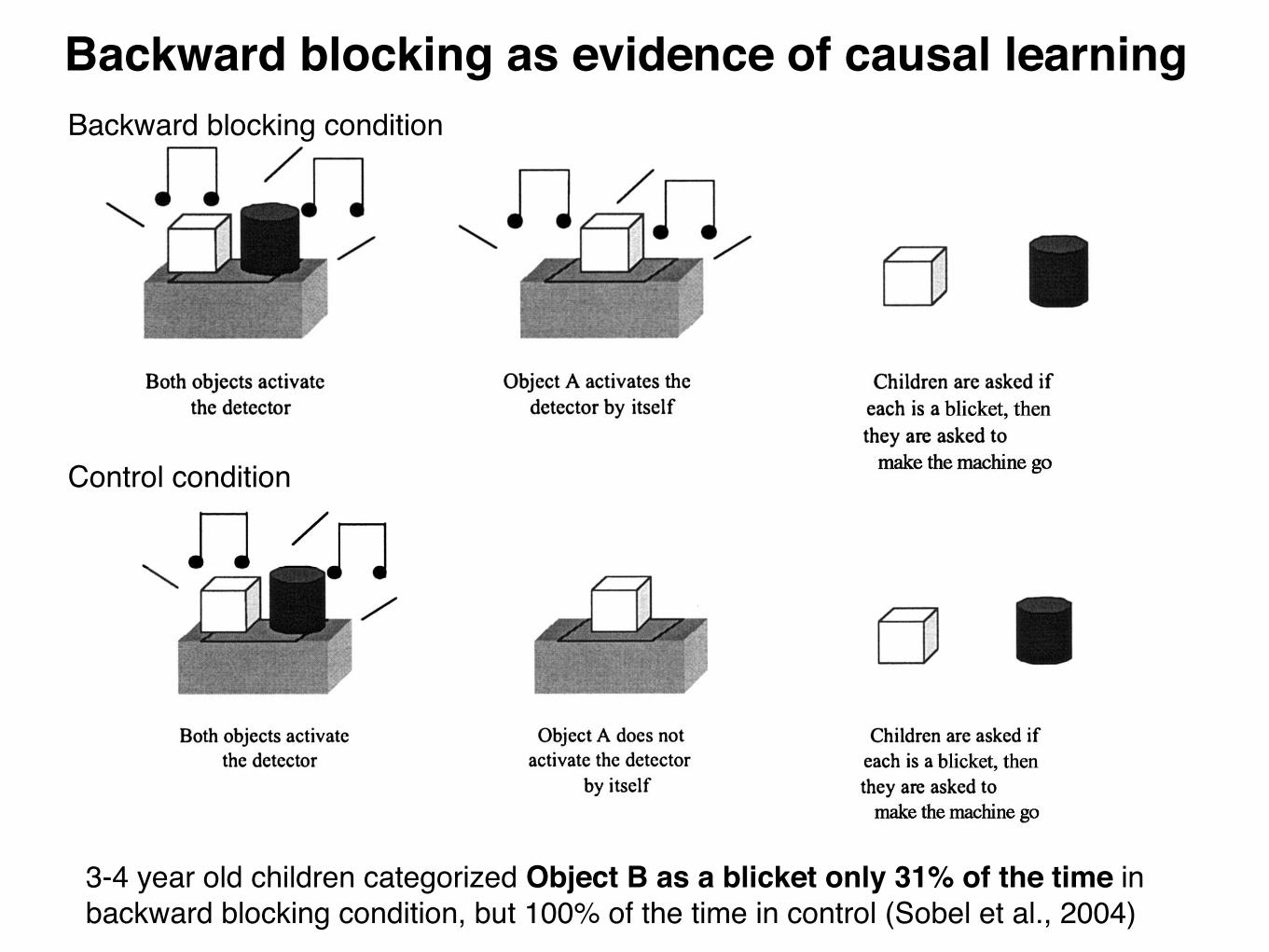
In the control, inference condition, children said that Object Awas a blicket only 6% of the time and always said that Object Bwas a blicket (100% of the time), significantly more often. Per-formance on the backward blocking condition was quite different:Children categorized Object A as a blicket 99% of the time.However, the critical question was how children would categorizeObject B. Overall, children categorized Object B as a blicket only31% of the time. In fact, even the youngest children categorizedObject B as a blicket significantly less often in the backwardblocking condition (50% of the time) than they did in the one-cause condition (100% of the time). In summary, children asyoung as 3 years old made different judgments about the causalpower of Object B, depending on what happened with Object A.They used the information from trials that just involved A to maketheir judgment about B.Children responded in a similar way to the “make it go” inter-
vention question. This question was analogous to the “make itstop” question in Gopnik et al. (2001). Children had never seen theexperimenter place the B block on the detector by itself in eithercondition. Nevertheless, in the inference condition they placed thisblock on the detector by itself 84% of the time. In the backwardblocking condition they did so 19% of the time, significantly lessoften, and significantly less often than they placed the A block onthe detector by itself (64% of the time).What would the various learning models predict about this
problem? In the pretest, children are shown that some blocks areblickets (about half the blocks, in fact). Children then have thefollowing data in the following sequence.Inference
1. A absent, B absent, E absent
2. A present, B present, E present
3. A present, B present, E present
4. A present, B absent, E absent
Backward blocking
1. A absent, B absent, E absent
2. A present, B present, E present
3. A present, B present, E present
4. A present, B absent, E present
According to the RW model, both A and B are positivelyassociated with E (the effect). The last trial, Trial 4, shouldstrengthen or weaken the association with A but should have noeffect on the association with B, because B is absent. If thatassociation is sufficiently strong, subjects should conclude thatboth A and B cause E. In particular, B should be equally stronglyassociated with E in the inference condition and the backwardblocking condition.In contrast, both Cheng’s (1997) learning rule, with a suitable
choice of focal sets, and constraint-based and Bayesian learningmethods yield a qualitative difference between A and B in thebackward blocking condition. In the RW model, the effect or lackof effect of the A block by itself has no influence on the judgmentabout B, but it has a crucial effect in these other models.According to Cheng’s (1997) methods, if the focal set for A in
the backward blocking condition consists of Cases 1 and 4 (so B
Figure 13. Procedure used in Sobel et al. (in press, Experiment 2).
23CAUSAL MAPS
Backward blocking as evidence of causal learning
3-4 year old children categorized Object B as a blicket only 31% of the time in backward blocking condition, but 100% of the time in control (Sobel et al., 2004)
In the control, inference condition, children said that Object Awas a blicket only 6% of the time and always said that Object Bwas a blicket (100% of the time), significantly more often. Per-formance on the backward blocking condition was quite different:Children categorized Object A as a blicket 99% of the time.However, the critical question was how children would categorizeObject B. Overall, children categorized Object B as a blicket only31% of the time. In fact, even the youngest children categorizedObject B as a blicket significantly less often in the backwardblocking condition (50% of the time) than they did in the one-cause condition (100% of the time). In summary, children asyoung as 3 years old made different judgments about the causalpower of Object B, depending on what happened with Object A.They used the information from trials that just involved A to maketheir judgment about B.Children responded in a similar way to the “make it go” inter-
vention question. This question was analogous to the “make itstop” question in Gopnik et al. (2001). Children had never seen theexperimenter place the B block on the detector by itself in eithercondition. Nevertheless, in the inference condition they placed thisblock on the detector by itself 84% of the time. In the backwardblocking condition they did so 19% of the time, significantly lessoften, and significantly less often than they placed the A block onthe detector by itself (64% of the time).What would the various learning models predict about this
problem? In the pretest, children are shown that some blocks areblickets (about half the blocks, in fact). Children then have thefollowing data in the following sequence.Inference
1. A absent, B absent, E absent
2. A present, B present, E present
3. A present, B present, E present
4. A present, B absent, E absent
Backward blocking
1. A absent, B absent, E absent
2. A present, B present, E present
3. A present, B present, E present
4. A present, B absent, E present
According to the RW model, both A and B are positivelyassociated with E (the effect). The last trial, Trial 4, shouldstrengthen or weaken the association with A but should have noeffect on the association with B, because B is absent. If thatassociation is sufficiently strong, subjects should conclude thatboth A and B cause E. In particular, B should be equally stronglyassociated with E in the inference condition and the backwardblocking condition.In contrast, both Cheng’s (1997) learning rule, with a suitable
choice of focal sets, and constraint-based and Bayesian learningmethods yield a qualitative difference between A and B in thebackward blocking condition. In the RW model, the effect or lackof effect of the A block by itself has no influence on the judgmentabout B, but it has a crucial effect in these other models.According to Cheng’s (1997) methods, if the focal set for A in
the backward blocking condition consists of Cases 1 and 4 (so B
Figure 13. Procedure used in Sobel et al. (in press, Experiment 2).
23CAUSAL MAPS
Backward blocking condition
Control condition
Neural network representation
A B
D
wA wB
In the control, inference condition, children said that Object Awas a blicket only 6% of the time and always said that Object Bwas a blicket (100% of the time), significantly more often. Per-formance on the backward blocking condition was quite different:Children categorized Object A as a blicket 99% of the time.However, the critical question was how children would categorizeObject B. Overall, children categorized Object B as a blicket only31% of the time. In fact, even the youngest children categorizedObject B as a blicket significantly less often in the backwardblocking condition (50% of the time) than they did in the one-cause condition (100% of the time). In summary, children asyoung as 3 years old made different judgments about the causalpower of Object B, depending on what happened with Object A.They used the information from trials that just involved A to maketheir judgment about B.Children responded in a similar way to the “make it go” inter-
vention question. This question was analogous to the “make itstop” question in Gopnik et al. (2001). Children had never seen theexperimenter place the B block on the detector by itself in eithercondition. Nevertheless, in the inference condition they placed thisblock on the detector by itself 84% of the time. In the backwardblocking condition they did so 19% of the time, significantly lessoften, and significantly less often than they placed the A block onthe detector by itself (64% of the time).What would the various learning models predict about this
problem? In the pretest, children are shown that some blocks areblickets (about half the blocks, in fact). Children then have thefollowing data in the following sequence.Inference
1. A absent, B absent, E absent
2. A present, B present, E present
3. A present, B present, E present
4. A present, B absent, E absent
Backward blocking
1. A absent, B absent, E absent
2. A present, B present, E present
3. A present, B present, E present
4. A present, B absent, E present
According to the RW model, both A and B are positivelyassociated with E (the effect). The last trial, Trial 4, shouldstrengthen or weaken the association with A but should have noeffect on the association with B, because B is absent. If thatassociation is sufficiently strong, subjects should conclude thatboth A and B cause E. In particular, B should be equally stronglyassociated with E in the inference condition and the backwardblocking condition.In contrast, both Cheng’s (1997) learning rule, with a suitable
choice of focal sets, and constraint-based and Bayesian learningmethods yield a qualitative difference between A and B in thebackward blocking condition. In the RW model, the effect or lackof effect of the A block by itself has no influence on the judgmentabout B, but it has a crucial effect in these other models.According to Cheng’s (1997) methods, if the focal set for A in
the backward blocking condition consists of Cases 1 and 4 (so B
Figure 13. Procedure used in Sobel et al. (in press, Experiment 2).
23CAUSAL MAPS
A B
D
A B
D
A B
D
A B
D
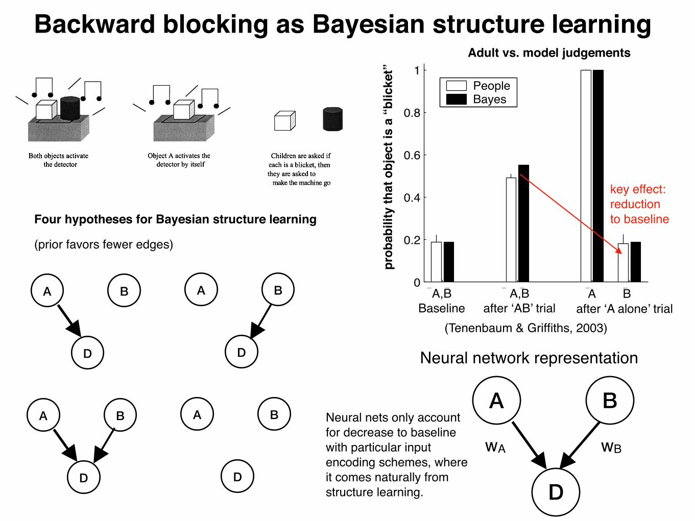
Four hypotheses for Bayesian structure learning
(prior favors fewer edges)
Backward blocking as Bayesian structure learning
Neural nets only account for decrease to baseline with particular input encoding schemes, where it comes naturally from structure learning.
X1X2
X1 X1
E E
h11 h00X2 X2
X(0)
E(1)
Z(1)
V(1)
E(0)
Z(0)
V(0)
E(n)
Z(n)
V(n)
...
...
t=0 t=1 t=n
hh1
0
presentabsent
E E
h h0110
X2X1
(a)
doorstate
vibrationalenergy
(b) blockposition
noise
time
Figure 1: Hypothesis spaces of causal Bayes nets for (a) the blicket detector and (b) themechanical vibration domains.
B1,B2 B1,B2 B1 B20
0.2
0.4
0.6
0.8
1(a)
Baseline After "12" trial
After "1 alone"
trial
B1,B2 B1,B2 B1 B20
0.2
0.4
0.6
0.8
1(b)
Baseline After "12" trial
After "1 alone"
trial
B1,B2,B3 B1,B2 B3 B1 B2,B30
0.2
0.4
0.6
0.8
1(c)
Baseline After "12" trial
After "13" trial
PeopleBayes
Figure 2: Human judgments and model predictions (based on Figure 1a) for one-shot back-wards blocking with blickets, when blickets are (a) rare or (b) common, or (c) rare and onlyobserved in ambiguous combinations. Bar height represents the mean judged probabilitythat an object has the causal power to activate the detector.
0.1 0.3 0.9 2.7 8.12
3
4
5
6
Time (sec)
Cau
sal s
treng
th
X = 15 X = 7 X = 3 X = 1
0.1 0.3 0.9 2.7 8.12
3
4
5
6
Time (sec)
P( h
1| T
, X)
0.1 0.3 0.9 2.7 8.12
3
4
5
6
Time (sec)
P( h
1| T
, X)
Figure 3: Probability of a causal connection between two events: a block dropping onto abeam and a trap door opening. Each curve corresponds to a different spatial gap betweenthese events; each x-axis value to a different temporal gap . (a) Human judgments. (b)Predictions of the dynamic Bayes net model (Figure 1b). (c) Predictions of the spatiotem-poral decay model.
A,BBaseline
A,Bafter ‘AB’ trial after ‘A alone’ trial
A B
Adult vs. model judgements
prob
abili
ty th
at o
bjec
t is
a “b
licke
t”
(Tenenbaum & Griffiths, 2003)
key effect: reduction to baseline
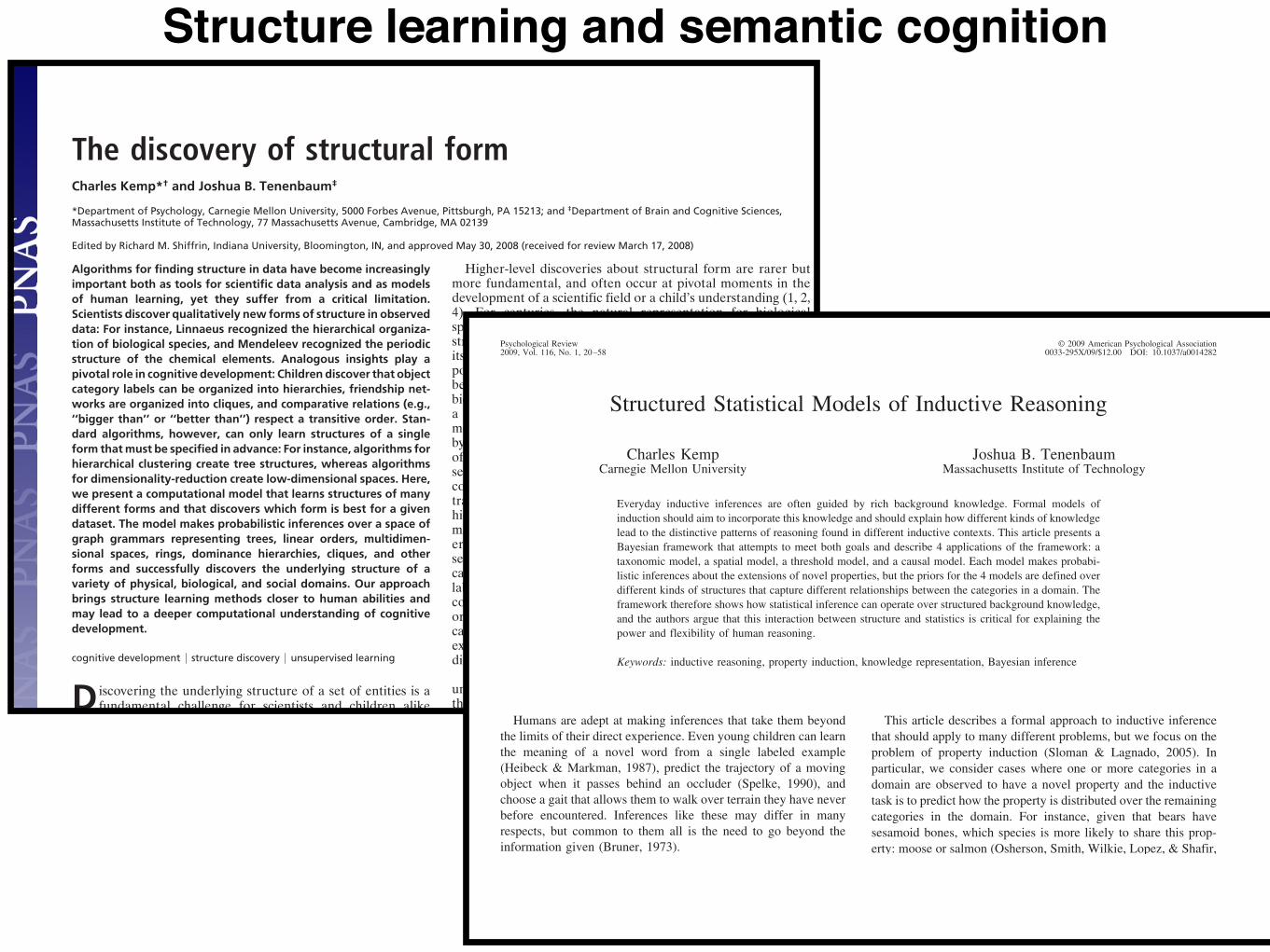
Structure learning and semantic cognition
The discovery of structural formCharles Kemp*† and Joshua B. Tenenbaum‡
*Department of Psychology, Carnegie Mellon University, 5000 Forbes Avenue, Pittsburgh, PA 15213; and ‡Department of Brain and Cognitive Sciences,Massachusetts Institute of Technology, 77 Massachusetts Avenue, Cambridge, MA 02139
Edited by Richard M. Shiffrin, Indiana University, Bloomington, IN, and approved May 30, 2008 (received for review March 17, 2008)
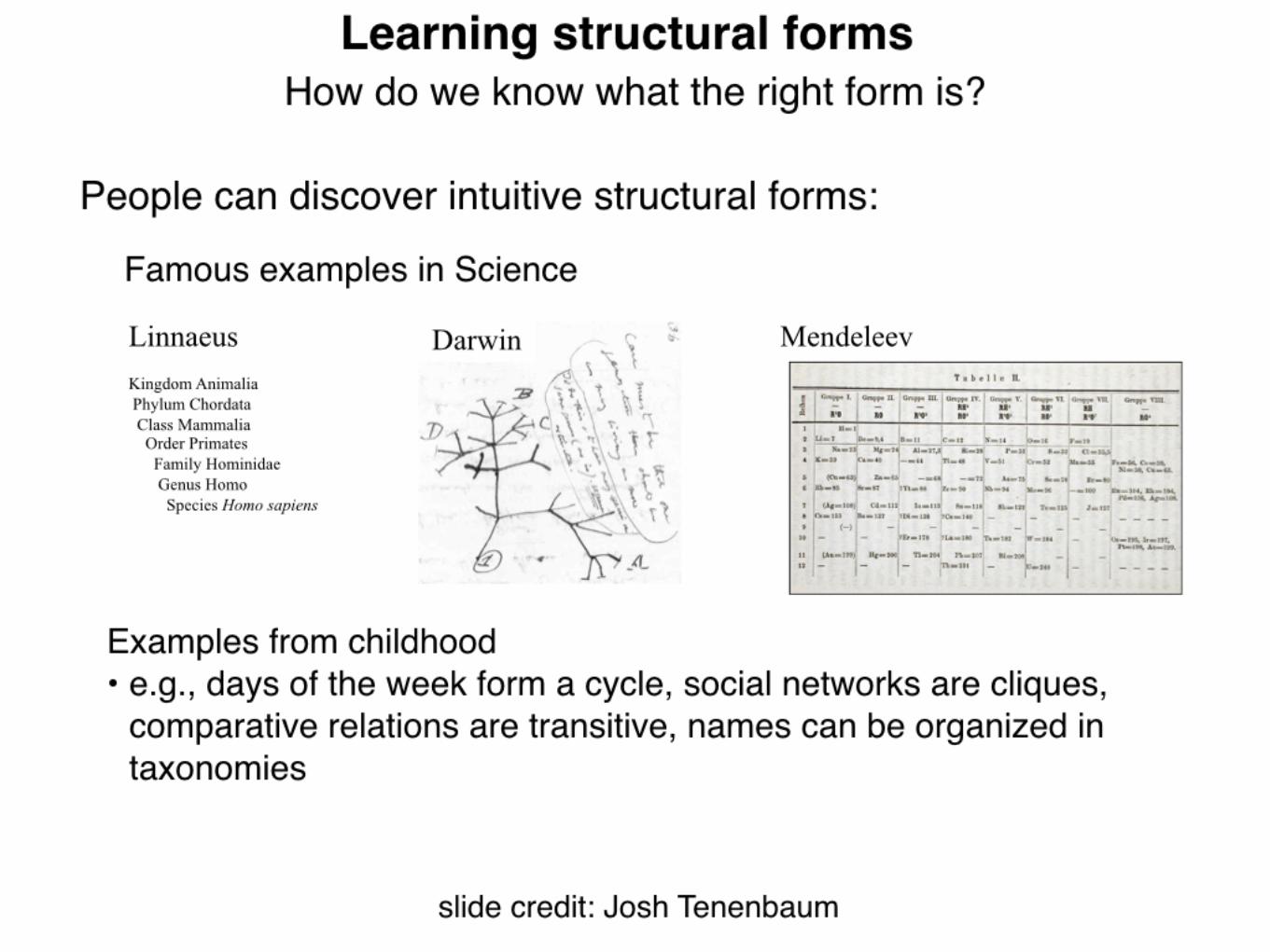
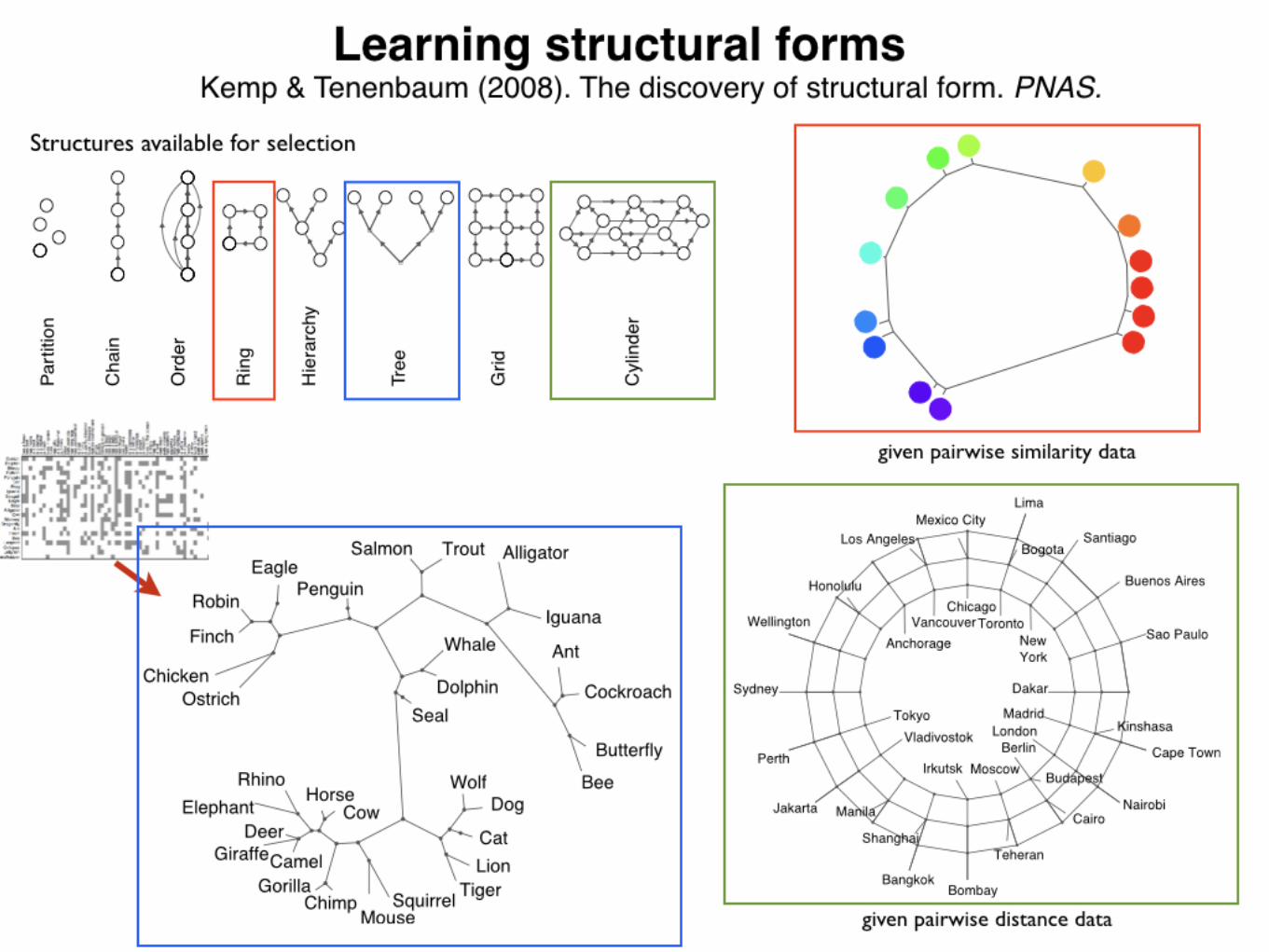
Algorithms for finding structure in data have become increasinglyimportant both as tools for scientific data analysis and as modelsof human learning, yet they suffer from a critical limitation.Scientists discover qualitatively new forms of structure in observeddata: For instance, Linnaeus recognized the hierarchical organiza-tion of biological species, and Mendeleev recognized the periodicstructure of the chemical elements. Analogous insights play apivotal role in cognitive development: Children discover that objectcategory labels can be organized into hierarchies, friendship net-works are organized into cliques, and comparative relations (e.g.,‘‘bigger than’’ or ‘‘better than’’) respect a transitive order. Stan-dard algorithms, however, can only learn structures of a singleform that must be specified in advance: For instance, algorithms forhierarchical clustering create tree structures, whereas algorithmsfor dimensionality-reduction create low-dimensional spaces. Here,we present a computational model that learns structures of manydifferent forms and that discovers which form is best for a givendataset. The model makes probabilistic inferences over a space ofgraph grammars representing trees, linear orders, multidimen-sional spaces, rings, dominance hierarchies, cliques, and otherforms and successfully discovers the underlying structure of avariety of physical, biological, and social domains. Our approachbrings structure learning methods closer to human abilities andmay lead to a deeper computational understanding of cognitivedevelopment.
cognitive development ! structure discovery ! unsupervised learning
D iscovering the underlying structure of a set of entities is afundamental challenge for scientists and children alike
(1–7). Scientists may attempt to understand relationships be-tween biological species or chemical elements, and children mayattempt to understand relationships between category labels orthe individuals in their social landscape, but both must solveproblems at two distinct levels. The higher-level problem is todiscover the form of the underlying structure. The entities maybe organized into a tree, a ring, a dimensional order, a set ofclusters, or some other kind of configuration, and a learner mustinfer which of these forms is best. Given a commitment to oneof these structural forms, the lower-level problem is to identifythe instance of this form that best explains the available data.
The lower-level problem is routinely confronted in science andcognitive development. Biologists have long agreed that treestructures are useful for organizing living kinds but continue todebate which tree is best—for instance, are crocodiles bettergrouped with lizards and snakes or with birds (8)? Similar issuesarise when children attempt to fit a new acquaintance into a setof social cliques or to place a novel word in an intuitive hierarchyof category labels. Inferences like these can be captured bystandard structure-learning algorithms, which search for struc-tures of a single form that is assumed to be known in advance(Fig. 1A). Clustering or competitive-learning algorithms (9, 10)search for a partition of the data into disjoint groups, algorithmsfor hierarchical clustering (11) or phylogenetic reconstruction(12) search for a tree structure, and algorithms for dimension-ality reduction (13, 14) or multidimensional scaling (15) searchfor a spatial representation of the data.
Higher-level discoveries about structural form are rarer butmore fundamental, and often occur at pivotal moments in thedevelopment of a scientific field or a child’s understanding (1, 2,4). For centuries, the natural representation for biologicalspecies was held to be the ‘‘great chain of being,’’ a linearstructure in which every living thing found a place according toits degree of perfection (16). In 1735, Linnaeus famously pro-posed that relationships between plant and animal species arebest captured by a tree structure, setting the agenda for allbiological classification since. Modern chemistry also began witha discovery about structural form, the discovery that the ele-ments have a periodic structure. Analogous discoveries are madeby children, who learn, for example, that social networks areoften organized into cliques, that temporal categories such as theseasons and the days of the week can be arranged into cycles, thatcomparative relations such as ‘‘longer than’’ or ‘‘better than’’ aretransitive (17, 18) and that category labels can be organized intohierarchies (19). Structural forms for some cognitive domainsmay be known innately, but many appear to be genuine discov-eries. When learning the meanings of words, children initiallyseem to organize objects into nonoverlapping clusters, with onecategory label allowed per cluster (20); hierarchies of categorylabels are recognized only later (19). When reasoning aboutcomparative relations, children’s inferences respect a transitiveordering by the age of 7 but not before (21). In both of thesecases, structural forms appear to be learned, but children are notexplicitly taught to organize these domains into hierarchies ordimensional orders.
Here, we show that discoveries about structural form can beunderstood computationally as probabilistic inferences aboutthe organizing principles of a dataset. Unlike most structure-learning algorithms (Fig. 1 A), the model we present can simul-taneously discover the structural form and the instance of thatform that best explain the data (Fig. 1B). Our approach canhandle many kinds of data, including attributes, relations, andmeasures of similarity, and we show that it successfully discoversthe structural forms of a diverse set of real-world domains.
Any model of form discovery must specify the space ofstructural forms it is able to discover. We represent structuresusing graphs and use graph grammars (22) as a unifyinglanguage for expressing a wide range of structural forms (Fig.2). Of the many possible forms, we assume that the mostnatural are those that can be derived from simple generativeprocesses (23). Each of the first six forms in Fig. 2 A can begenerated by using a single context-free production thatreplaces a parent node with two child nodes and specifies howto connect the children to each other and to the neighbors of
Author contributions: C.K. and J.B.T. designed research; C.K. performed research; and C.K.and J.B.T. wrote the paper.
The authors declare no conflict of interest.
This article is a PNAS Direct Submission.†To whom correspondence should be addressed. E-mail: [email protected].
Freely available online through the PNAS open access option.
See Commentary on page 10637.
This article contains supporting information online at www.pnas.org/cgi/content/full/0802631105/DCSupplemental.
© 2008 by The National Academy of Sciences of the USA
www.pnas.org"cgi"doi"10.1073"pnas.0802631105 PNAS ! August 5, 2008 ! vol. 105 ! no. 31 ! 10687–10692
COM
PUTE
RSC
IEN
CES
PSYC
HOLO
GY
SEE
COM
MEN
TARY
Structured Statistical Models of Inductive Reasoning
Charles KempCarnegie Mellon University
Joshua B. TenenbaumMassachusetts Institute of Technology
Everyday inductive inferences are often guided by rich background knowledge. Formal models ofinduction should aim to incorporate this knowledge and should explain how different kinds of knowledgelead to the distinctive patterns of reasoning found in different inductive contexts. This article presents aBayesian framework that attempts to meet both goals and describe 4 applications of the framework: ataxonomic model, a spatial model, a threshold model, and a causal model. Each model makes probabi-listic inferences about the extensions of novel properties, but the priors for the 4 models are defined overdifferent kinds of structures that capture different relationships between the categories in a domain. Theframework therefore shows how statistical inference can operate over structured background knowledge,and the authors argue that this interaction between structure and statistics is critical for explaining thepower and flexibility of human reasoning.
Keywords: inductive reasoning, property induction, knowledge representation, Bayesian inference
Humans are adept at making inferences that take them beyondthe limits of their direct experience. Even young children can learnthe meaning of a novel word from a single labeled example(Heibeck & Markman, 1987), predict the trajectory of a movingobject when it passes behind an occluder (Spelke, 1990), andchoose a gait that allows them to walk over terrain they have neverbefore encountered. Inferences like these may differ in manyrespects, but common to them all is the need to go beyond theinformation given (Bruner, 1973).
Two different ways of going beyond the available informationcan be distinguished. Deductive inferences draw out conclusionsthat may have been previously unstated but were implicit in thedata provided. Inductive inferences go beyond the available data ina more fundamental way and arrive at conclusions that are likelybut not certain given the available evidence. Both kinds of infer-ences are of psychological interest, but inductive inferences appearto play a more central role in everyday cognition. We have alreadyseen examples related to language, vision, and motor control, andmany other inductive problems have been described in the litera-ture (Anderson, 1990; Holland, Holyoak, Nisbett, & Thagard,1986).
This article describes a formal approach to inductive inferencethat should apply to many different problems, but we focus on theproblem of property induction (Sloman & Lagnado, 2005). Inparticular, we consider cases where one or more categories in adomain are observed to have a novel property and the inductivetask is to predict how the property is distributed over the remainingcategories in the domain. For instance, given that bears havesesamoid bones, which species is more likely to share this prop-erty: moose or salmon (Osherson, Smith, Wilkie, Lopez, & Shafir,1990; Rips, 1975)? Moose may seem like the better choice becausethey are more similar biologically to bears, but different propertiescan lead to different patterns of inference. For example, given thata certain disease is found in bears, it may seem more likely that thedisease is found in salmon than in moose—perhaps the bearspicked up the disease from something they ate.
As these examples suggest, inferences about different propertiescan draw on very different kinds of knowledge. A psychologicalaccount of induction should answer at least two questions—what isthe nature of the background knowledge that supports induction,and how is that knowledge combined with evidence to yield aconclusion? The first challenge is to handle the diverse forms ofknowledge that are relevant to different problems. For instance,inferences about an anatomical property like sesamoid bones maybe guided by knowledge about the taxonomic relationships be-tween biological species, but inferences about a novel disease maybe guided by ecological relationships between species, such aspredator–prey relations. The second challenge is to explain howthis knowledge guides induction. For instance, we need to explainhow knowledge about ecological relationships (“bears eatsalmon”) is combined with evidence (“salmon have a disease”) toarrive at a conclusion (“bears are likely to carry the disease”).
Existing accounts of property induction usually emphasize justone of the questions we have identified. Theory-based approaches(Carey, 1985; Murphy & Medin, 1985) focus on the first questionand attempt to characterize the knowledge that supports induction.Studies in this tradition have established that induction often drawson intuitive theories, or systems of rich conceptual knowledge, and
Charles Kemp, Department of Psychology, Carnegie Mellon University;Joshua B. Tenenbaum, Department of Brain and Cognitive Science, Mas-sachusetts Institute of Technology.
This work was supported in part by the Air Force Office of ScientificResearch under contracts FA9550-05-1-0321 and FA9550-07-2-0351.Charles Kemp was supported by the William Asbjornsen Albert MemorialFellowship, and Joshua B. Tenenbaum was supported by the Paul E.Newton Chair. Many of the ideas in this article were developed in collab-orations with Neville Sanjana, Patrick Shafto, Elizabeth Baraff-Bonawitz,and John Coley. We thank Erik Sudderth and Bob Rehder for valuablediscussions, Sergey Blok and collaborators for sharing data described inBlok et al. (2007), and Steven Sloman for sharing his copy of the featuredata described in Osherson et al. (1991).
Correspondence concerning this article should be sent to Charles Kemp,5000 Forbes Avenue, Baker Hall 340T, Pittsburgh, PA 15217. E-mail:[email protected]
Psychological Review © 2009 American Psychological Association2009, Vol. 116, No. 1, 20–58 0033-295X/09/$12.00 DOI: 10.1037/a0014282
20

© 2003 Nature Publishing Group
314 | APRIL 2003 | VOLUME 4 www.nature.com/reviews/neuro
R E V I EW S
children’s experience, and the coding of experience forthe network finesses some important issues. However,we argue that the training data capture two essential fea-tures. First, many types of naturally occurring thingshave a hierarchical similarity structure, as Quilliannoticed; and second, from exposure to examples ofobjects children learn just what the similarities are andhow they can be exploited.
The Rumelhart model can show how learning canshape not only overt responses, but also internal repre-sentations. A special set of internal or hidden units,labelled ‘representation’ units, was included between theinput units for the individual concepts and the largegroup of hidden units that combine the concept andrelation information. When the network is initialized,the patterns of activation on the representation units areweak and random, owing to the random initial connec-tion weights, but gradually these patterns become differentiated, recapitulating the general-to-specificprogression seen in many developmental studies. Thesimulation results in FIG. 4 show that patterns represent-ing the different concepts are similar at the beginningof training, but gradually become differentiated inwaves. One wave of differentiation separates plants fromanimals. The next waves differentiate birds from fish,and trees from flowers. Later waves differentiate theindividual objects. The process is continuous, but thereare periods of stability punctuated by relatively rapidtransitions also seen in many other developmentalmodels54,56,59, reminiscent of the seemingly stage-likecharacter of many aspects of cognitive development62.
Rumelhart focused on showing how this networkrecapitulates Quillian’s hierarchical representation ofconcepts, but in a different way than Quillian envi-sioned it — in the pattern of similarities and differencesamong the internal representations of the various con-cepts, rather than in the form of explicit ‘ISA’ links. Thischaracteristic of the model is clearly brought out in thehierarchical clustering analysis of the representations ofthe concepts (FIG. 4b). Rumelhart also showed how thenetwork could generalize what it knows about familiarconcepts to new ones. He introduced the network to anew concept,‘sparrow’, by adding a new input unit with0-valued connections to the representation units. Hethen presented the network with the input–output pair‘sparrow–ISA–bird/animal/living thing’. Only the con-nection weights from ‘sparrow’ to the representationunits were allowed to change. As a result, ‘sparrow’ pro-duced a pattern of activation similar to that already usedfor the robin and the canary. Rumelhart then tested theresponses of the network to other questions about thesparrow, by probing with the inputs ‘sparrow–CAN’,‘sparrow–HAS’ and ‘sparrow–IS’. In each case the net-work activated output units corresponding to sharedcharacteristics of the other birds in the training set(CAN grow, CAN move, CAN fly; HAS skin, HASwings, HAS feathers), and produced very low activationof output units corresponding to attributes not charac-teristic of any animals. Attributes varying between thebirds and attributes possessed by other animals receivedintermediate degrees of activation. This behaviour is a
compared to the correct output (activation of ‘grow’,‘move’,‘fly’ and ‘sing’ should be 1, and activation of otheroutput units should be 0). The connection weights arethen adjusted to reduce the difference between the tar-get and the obtained activations. The set of trainingexperiences includes one for each concept–relation pair,with the target specifying all valid completions consis-tent with FIG. 1.
The network is trained through many epochs or suc-cessive sweeps through the set of training examples.Only small adjustments to the connection weights aremade after each example is processed, so that learning isvery gradual — akin to the process we believe occurs indevelopment, as children experience items and theirproperties through day-to-day experience. Of course,the tiny training set used is not fully representative of
Skin
Roots
Gills
Scales
Feathers
Wings
Petals
Bark
Sing
Yellow
Fly
Swim
Move
Grow
Red
Green
Tall
Living
Pretty
Salmon
Sunfish
Canary
Robin
Daisy
Rose
Oak
Pine
Flower
Bird
Flower
Tree
Animal
Living thing
Plant
Relation
Attribute
Item
ISA
IS
CAN
HAS
Salmon
Sunfish
Canary
Robin
Daisy
Rose
Oak
PineHiddenRepresentation
Figure 3 | Our depiction of the connectionist network used by Rumelhart60,61. The networkis used to learn propositions about the concepts shown in FIG. 1. The entire set of units used inthe network is shown. Inputs are presented on the left, and activation propagates from left toright. Where connections are indicated, every unit in the pool on the left (sending) side projects toevery unit on the right (receiving) side. An input consists of a concept–relation pair; the input‘canary CAN’ is represented by darkening the active input units. The network is trained to turn onall those output units that represent correct completions of the input pattern. In this case, thecorrect units to activate are ‘grow’, ‘move’, ‘fly’ and ‘sing’. Subsequent analysis focuses on theconcept representation units, the group of eight units to the right of the concept input units.Adapted, with permission, from REF. 61 © (1993) MIT Press.
Review: A neural network model of semantic cognition
• Network is trained to answer queries involving an item (e.g., “Canary”) and a relation (e.g., “CAN”), outputting all attributes that are true of the item/relation pair (e.g., “grow, move, fly, sing”)
• Trained with stochastic gradient descent, as we learned about in this lecture
• The model helps us to understand the broad-to-specific pattern of differentiation in children’s cognitive development
• It also helps us to understand the specific-to-general deterioration in semantic dementia

property induction as probabilistic inference:
P (fY = 1|fX = 1) Y = {horses}
X = {cows, seals}
f : T9 hormones
Question: “Given that cows and seals have T9 hormones, how likely is it that horses do?”
Alternative: Property induction as probabilistic inference in a probabilistic graphical model
Features!
Horse!Cow!
Chimp!Gorilla!Mouse!Squirrel!Dolphin!
Seal!Rhino!
Elephant!
f (1) f (m)f (2), ...,
Structure
Data f (k)
S
argmaxS
p(S|f (1), ..., f (k)) �mY
i=1
p(f (i)|S)p(S)
Find structure S that maximizes the objective function:
Features!
Horse!Cow!
Chimp!Gorilla!Mouse!Squirrel!Dolphin!
Seal!Rhino!
Elephant!
f (1) f (m)f (2), ...,
dolphin
squirrel
seal
elephant
rhino
chimp
gorilla
mouse
(Gaussian Markov Random Fieldwith latent variables)
observed variable(object)
latent variable
Key
Likelihood favors fit to the data
Prior favors sparse graphs
Structural sparsity algorithm for discovering organizing structure in data
(Lake, Lawrence, & Tenenbaum, under review)?!
?!?!?!?!?!
?!?!
Features! New property!
?
Horse!Cow!
Chimp!Gorilla!Mouse!
Squirrel!Dolphin!
Seal!Rhino!
Elephant!
Property induction
“Given that cows and seals have T9 hormones, how likely is it that horses do?”
Features for Elephant: ‘gray’, ‘hairless’, ‘toughskin’, ‘big’, ‘bulbous’, ‘longleg’, ‘tail’, ‘chewteeth’, ‘tusks’, ‘smelly’, ‘walks’, ‘slow’, ‘strong’, ‘muscle’, ‘fourlegs’,…
f (1)f (m)f (2), ...,
new property
background data graphical model structure learning
property induction as prob. inference
Bayesian modeling roadmap
Features for Elephant: ‘gray’, ‘hairless’, ‘toughskin’, ‘big’, ‘bulbous’, ‘longleg’, ‘tail’, ‘chewteeth’, ‘tusks’, ‘smelly’, ‘walks’, ‘slow’, ‘strong’, ‘muscle’, ‘fourlegs’,…
P (fY = 1|fX = 1)

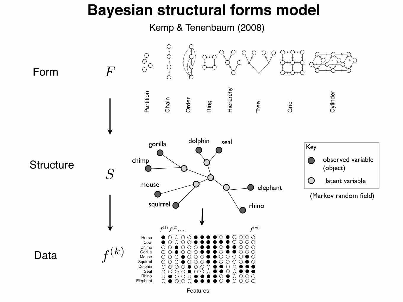
Structure
Data f (k)
S
Features!
Horse!Cow!
Chimp!Gorilla!Mouse!Squirrel!Dolphin!
Seal!Rhino!
Elephant!
f (1) f (m)f (2), ...,
dolphin
squirrel
seal
elephant
rhino
chimp
gorilla
mouse
(Markov random field)
observed variable(object)
latent variable
Key
Bayesian structural forms model
Form
the
pare
ntno
de.
Fig.
2B
–Dsh
ows
how
thre
eof
thes
epr
oduc
tions
gene
rate
chai
ns,o
rder
s,an
dtr
ees.
Mor
eco
mpl
exfo
rms,
incl
udin
gm
ultid
imen
sion
alsp
aces
and
cylin
ders
,can
bege
nera
ted
byco
mbi
ning
thes
eba
sic
form
sor
byus
ing
mor
eco
mpl
expr
oduc
tions
.It
isst
riki
ngth
atth
esi
mpl
egr
amm
ars
inFi
g.2A
gene
rate
man
yof
the
stru
ctur
alfo
rmsd
iscu
ssed
byps
ycho
logi
sts(
24)a
ndas
sum
edby
algo
rith
msf
orun
supe
rvis
edle
arni
ngor
expl
orat
ory
data
anal
ysis
.Par
titio
ns(9
,25)
,cha
ins
(26)
,ord
ers
(1,2
5,27
),ri
ngs(
28,2
9),t
rees
(1,1
2,30
),hi
erar
chie
s(31
,32)
and
grid
s(33
)re
cur
agai
nan
dag
ain
info
rmal
mod
els
acro
ssm
any
diff
eren
tlit
erat
ures
.To
high
light
just
one
exam
ple,
Inhe
lder
and
Piag
et(1
)su
gges
tth
atth
eel
emen
tary
logi
calo
pera
tions
inch
ildre
n’s
thin
king
are
foun
ded
ontw
ofo
rms:
acl
assi
ficat
ion
stru
ctur
eth
atca
nbe
mod
eled
asa
tree
and
ase
riat
ion
stru
ctur
eth
atca
nbe
mod
eled
asan
orde
r.T
hepo
pula
rity
ofth
efo
rms
inFi
g.2
sugg
ests
that
they
are
usef
ulfo
rde
scri
bing
the
wor
ld,a
ndth
atth
eysp
ring
tom
ind
natu
rally
whe
nsc
ient
ists
seek
form
alde
-sc
ript
ions
ofa
dom
ain.
The
prob
lem
offo
rmdi
scov
ery
can
now
bepo
sed.
Giv
enda
taD
abou
ta
finite
set
ofen
titie
s,w
ew
ant
tofin
dth
efo
rmF
and
the
stru
ctur
eS
ofth
atfo
rmth
atbe
stca
ptur
eth
ere
latio
nshi
psbe
twee
nth
ese
entit
ies.
We
take
apr
obab
ilist
icap
proa
ch,
and
defin
ea
hier
arch
ical
gene
rativ
em
odel
(34)
that
spec
ifies
how
the
data
are
gene
rate
dfr
oman
unde
rlyi
ngst
ruct
ure,
and
how
this
stru
ctur
eis
gene
rate
dfr
oman
unde
rlyi
ngfo
rm(F
ig.1
B).
We
then
sear
chfo
rth
est
ruct
ure
San
dfo
rmF
that
max
imiz
eth
epo
ster
ior
prob
abili
ty
P!S,
F!D
"#
P!D
!S"P
!S!F
"P!F
".[1
]
P(F)
isa
unifo
rmdi
stri
butio
nov
erth
efo
rms
unde
rco
nsid
er-
atio
n(F
ig.2
).St
ruct
ure
Sis
acl
uste
rgr
aph,
anin
stan
ceof
one
ofth
efo
rms
inFi
g.2,
whe
reth
eno
des
repr
esen
tcl
uste
rsof
entit
ies(
Fig.
4Ash
owsa
clus
terg
raph
with
the
form
ofan
orde
r).
The
prio
rP(
S!F)
favo
rsgr
aphs
whe
rek,
the
num
ber
ofcl
uste
rs,
issm
all:
P(S!
F)#
!kif
Sis
com
patib
lew
ithF,
and
P(S!
F)$
0ot
herw
ise
[see
supp
ortin
gin
form
atio
n(S
I)A
ppen
dix
for
the
defin
ition
ofco
mpa
tibili
ty].
The
para
met
er!
dete
rmin
esth
e
croco
dilebat
gorill
a
ostric
hro
bin
turtle
snak
ePCA,
MDS
Hierarchical
clustering
robin
ostric
h
croco
dile
snak
etur
tlebat
gorill
a
Unidimensional
scaling
ostric
hgorill
a
croco
dile
turtle
robin
bat
snak
e
bat
ostric
hro
bin turtle
gorill
acro
codil
esn
ake
croco
dile turtle
snak
e
robin
ostric
hgo
rilla
bat
gorill
asn
ake
turtle
bat
robin
ostric
hcro
codil
e
gorill
a bat
turtle
sn
ake
croco
dile
robi n
os
trich
f 1 f 2
f 3 f 4
f 5 f 10
0 ......
...
gorill
a bat
turtle
sn
ake
croco
dile
robi n
os
tric h
f 1 f 2
f 3 f 4
f 5 f 10
0 ......
...
Clustering
Data
Stru
cture
Form
Tree
Circumplex
models
A
Minimum
B
spanning
tree
robin
ostric
h
croco
dile
snak
etur
tlebat
gorill
a
Fig.
1.Fi
ndin
gst
ruct
ure
inda
ta.(
A)S
tand
ard
stru
ctur
ele
arni
ngal
gori
thm
sse
arch
for
repr
esen
tati
ons
ofa
sing
lefo
rmth
atis
fixe
din
adva
nce.
Show
nhe
rear
em
etho
dsth
atdi
scov
ersi
xdi
ffer
entk
inds
ofst
ruct
ures
give
na
mat
rix
ofbi
nary
feat
ures
.(B)
Ahi
erar
chic
alm
odel
that
disc
over
sthe
form
Fan
dth
est
ruct
ure
Sth
atbe
stac
coun
tfo
rth
eda
taD
.The
mod
else
arch
esfo
rth
efo
rman
dst
ruct
ure
that
join
tly
max
imiz
eP(
S,F!
D)#
P(D
!S)P
(S!F
)P(F
). D
⇒⇒⇒⇒⇒ ⇒⇒ ⇒ ⇒ ⇒
C
St ru
ctur a
l Fo r
m
Gene
rativ
ep
roce
ss
Pa rt i
tio n
⇒
Chai n
⇒
Orde
r ⇒
Ring
⇒
Hier
arch
y ⇒
Tr ee
⇒
Gr id
Chai n
Ch
ai n
Cylin
der
Chai n
Ri
ng
AB
∏ ∏
Fig.
2.A
hypo
thes
issp
ace
ofst
ruct
ural
form
s.(A
)Eig
htst
ruct
ural
form
sand
the
gene
rati
vepr
oces
sest
hatp
rodu
ceth
em.O
pen
node
srep
rese
ntcl
uste
rsof
obje
cts:
Ahi
erar
chy
has
obje
cts
loca
ted
inte
rnal
ly,b
uta
tree
may
only
have
obje
cts
atit
sle
aves
.Th
efi
rst
six
proc
esse
sar
eno
de-r
epla
cem
ent
grap
hgr
amm
ars.
Each
gram
mar
uses
asi
ngle
prod
ucti
on,
and
each
prod
ucti
onsp
ecifi
esho
wto
repl
ace
apa
rent
node
wit
htw
och
ildno
des.
The
seed
fore
ach
gram
mar
isa
grap
hw
ith
asi
ngle
node
(inth
eca
seof
the
ring
,thi
sno
deha
sa
self
-link
).(B
–D)
Gro
win
gch
ains
,or
ders
,an
dtr
ees.
At
each
step
inea
chde
riva
tion
,the
pare
ntan
dch
ildno
des
are
show
nin
gray
.The
grap
hge
ner-
ated
atea
chst
epis
ofte
nre
arra
nged
befo
reth
ene
xtst
ep.I
nB,
for
inst
ance
,th
eri
ghts
ide
ofth
efi
rsts
tep
and
the
left
side
ofth
ese
cond
step
are
iden
tica
lgr
aphs
.The
red
arro
ws
inea
chpr
oduc
tion
repr
esen
tal
ledg
esth
aten
ter
orle
ave
apa
rent
node
.W
hen
appl
ying
the
orde
rpr
oduc
tion
,al
lno
des
that
prev
ious
lyse
nta
link
toth
epa
rent
node
now
send
links
tobo
thch
ildre
n.
1068
8!
ww
w.p
nas.
org"
cgi"
doi"
10.1
073"
pnas
.080
2631
105
Kem
pan
dTe
nenb
aum
F
Kemp & Tenenbaum (2008)
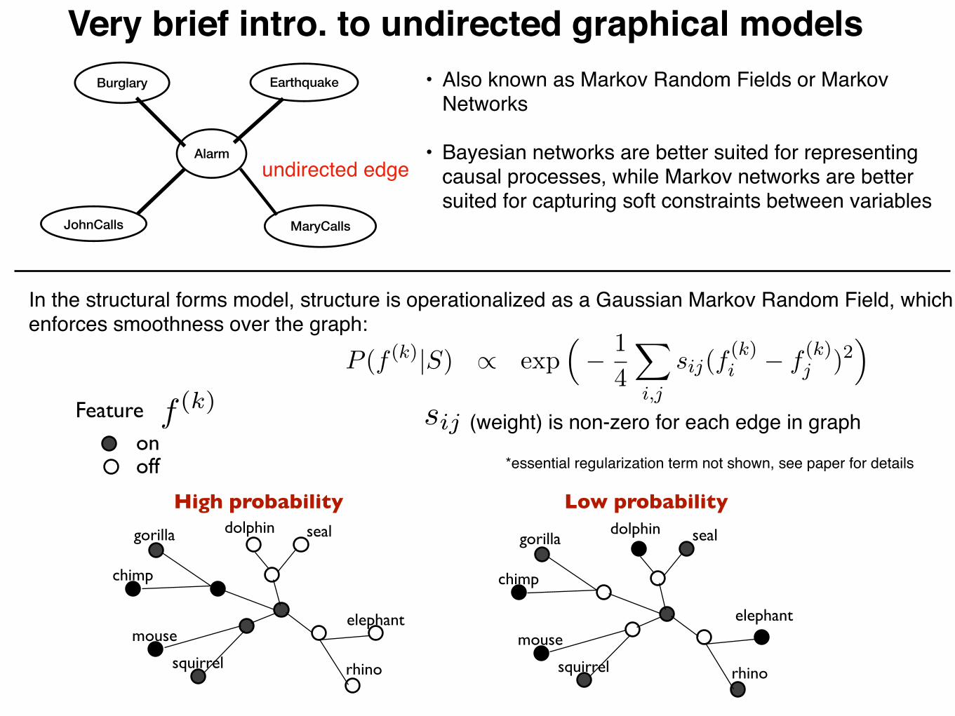
dolphin
squirrel
seal
elephant
rhino
chimp
gorilla
mouse
dolphin
squirrel
seal
elephant
rhino
chimp
gorilla
mouse
Feature f (k)
onoff
High probability Low probability
Very brief intro. to undirected graphical modelsBurglary Earthquake
Alarm
JohnCalls MaryCalls
• Also known as Markov Random Fields or Markov Networks
• Bayesian networks are better suited for representing causal processes, while Markov networks are better suited for capturing soft constraints between variables
In the structural forms model, structure is operationalized as a Gaussian Markov Random Field, which enforces smoothness over the graph:
given by �S and its diagonal elements are
�ii =X
j
sij .
A generative model for features can then be written as
P (f (k)|S) / exp⇣� 1
4
X
i,j
sij(f(k)i � f
(k)j )2
⌘
= exp⇣� 1
2f(k)>�f
(k)⌘.
This equation highlights why the model favors features that are smooth across the graph. Features
are probable when connected objects i and j (sij > 0) have a similar value. The stronger the
connection sij (meaning the larger its value), the more important it is for the feature values to
match. As pointed out in Zhu et al. (2003), this distribution is not proper, since adding a constant
value to the feature vector does not change its probability. Therefore following Zhu et al. (2003),
we define the matrix J = �+ 1�2 I and use
P (f (k)|S,�2) / exp⇣� 1
2f(k)>
Jf(k)
⌘, (1)
which results in a proper density. This distribution is an nt dimensional Gaussian with zero mean
P (f (k)|S,�2) = N
⇣f(k)|0, J�1
⌘
=1
(2⇡)nt/2|J |�1/2exp
⇣� 1
2f(k)>
Jf(k)
⌘.
This generative model for features can also be derived from a maximum entropy formulation, as
shown in Lawrence (2011, 2012). This distribution over features is nearly the same as in the
structural forms model, except the forms model adds the diagonal term 1�2 only to the observed
nodes.
This distribution is also known as a Gaussian Markov Random Field (Koller & Friedman, 2009).
The undirected graph S (and equivalently the precision matrix J) instantiates a set of conditional
2
sij (weight) is non-zero for each edge in graph
undirected edge
*essential regularization term not shown, see paper for details
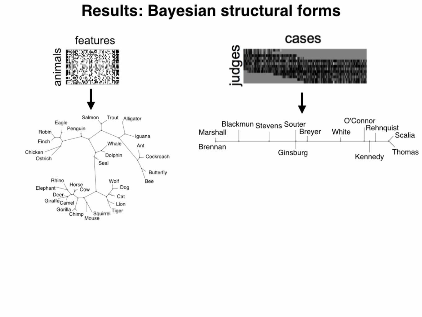
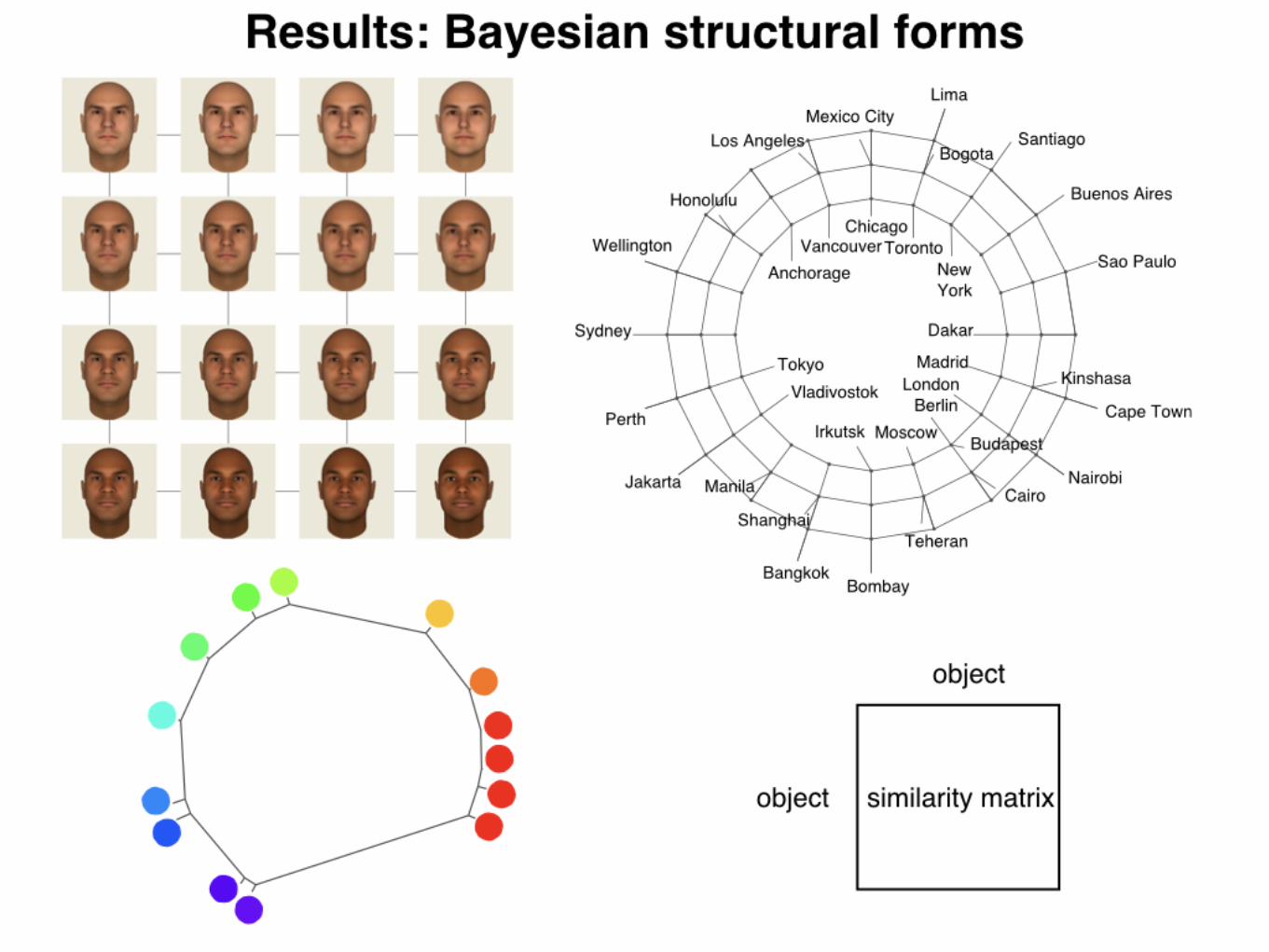
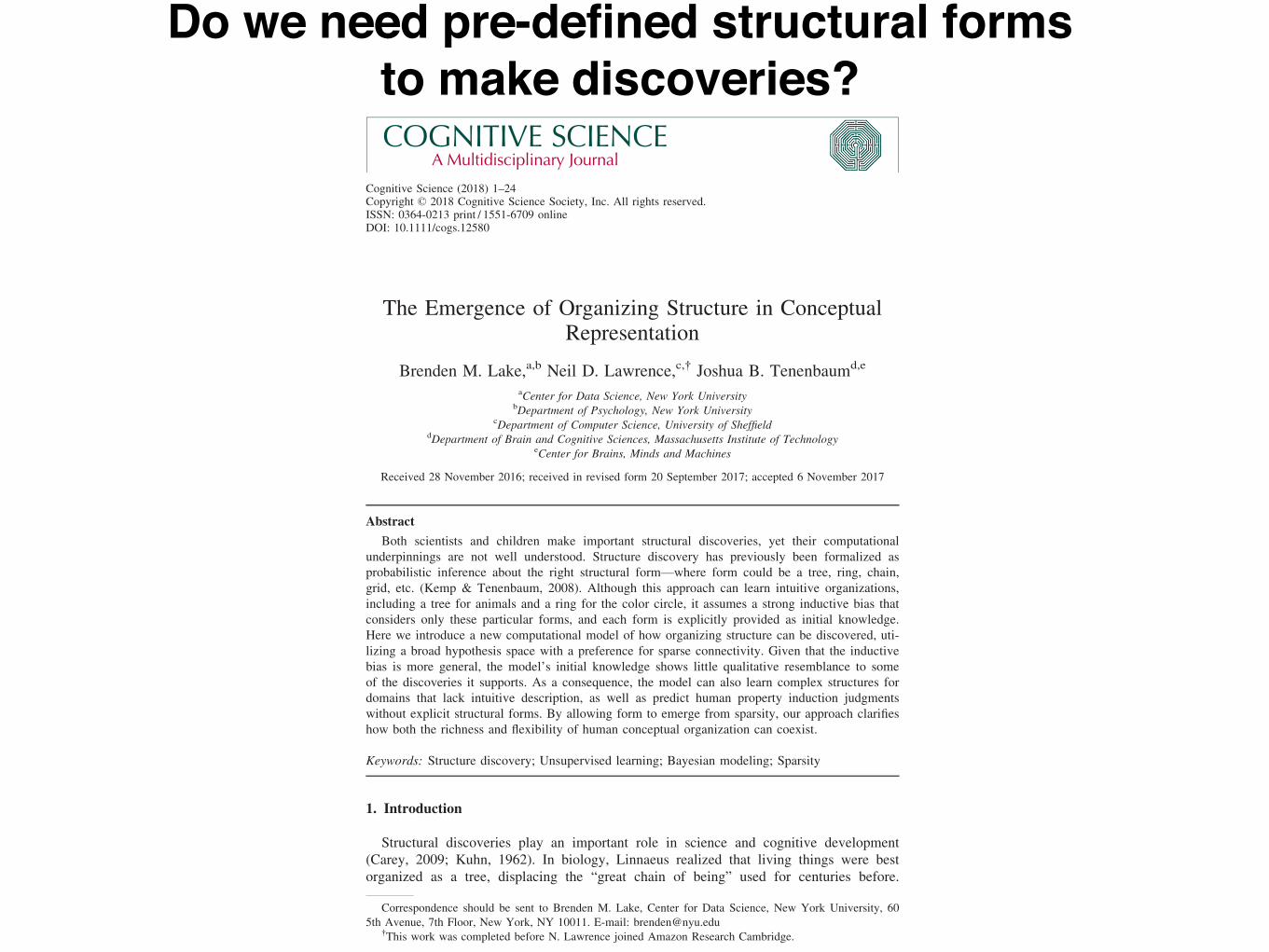
Cognitive Science (2018) 1–24Copyright © 2018 Cognitive Science Society, Inc. All rights reserved.ISSN: 0364-0213 print / 1551-6709 onlineDOI: 10.1111/cogs.12580
The Emergence of Organizing Structure in ConceptualRepresentation
Brenden M. Lake,a,b Neil D. Lawrence,c,† Joshua B. Tenenbaumd,e
aCenter for Data Science, New York UniversitybDepartment of Psychology, New York University
cDepartment of Computer Science, University of SheffielddDepartment of Brain and Cognitive Sciences, Massachusetts Institute of Technology
eCenter for Brains, Minds and Machines
Received 28 November 2016; received in revised form 20 September 2017; accepted 6 November 2017
Abstract
Both scientists and children make important structural discoveries, yet their computationalunderpinnings are not well understood. Structure discovery has previously been formalized asprobabilistic inference about the right structural form—where form could be a tree, ring, chain,grid, etc. (Kemp & Tenenbaum, 2008). Although this approach can learn intuitive organizations,including a tree for animals and a ring for the color circle, it assumes a strong inductive bias thatconsiders only these particular forms, and each form is explicitly provided as initial knowledge.Here we introduce a new computational model of how organizing structure can be discovered, uti-lizing a broad hypothesis space with a preference for sparse connectivity. Given that the inductivebias is more general, the model’s initial knowledge shows little qualitative resemblance to someof the discoveries it supports. As a consequence, the model can also learn complex structures fordomains that lack intuitive description, as well as predict human property induction judgmentswithout explicit structural forms. By allowing form to emerge from sparsity, our approach clarifieshow both the richness and flexibility of human conceptual organization can coexist.
Keywords: Structure discovery; Unsupervised learning; Bayesian modeling; Sparsity
1. Introduction
Structural discoveries play an important role in science and cognitive development(Carey, 2009; Kuhn, 1962). In biology, Linnaeus realized that living things were bestorganized as a tree, displacing the “great chain of being” used for centuries before.
Correspondence should be sent to Brenden M. Lake, Center for Data Science, New York University, 605th Avenue, 7th Floor, New York, NY 10011. E-mail: [email protected]
†This work was completed before N. Lawrence joined Amazon Research Cambridge.
Do we need pre-defined structural forms to make discoveries?
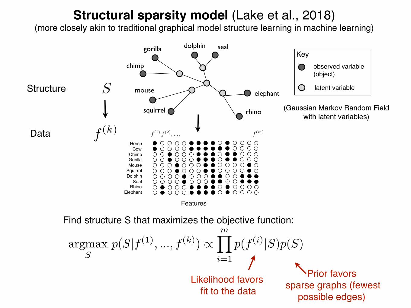
Structure
Data f (k)
S
argmaxS
p(S|f (1), ..., f (k)) �mY
i=1
p(f (i)|S)p(S)
Find structure S that maximizes the objective function:
Features!
Horse!Cow!
Chimp!Gorilla!Mouse!Squirrel!Dolphin!
Seal!Rhino!
Elephant!
f (1) f (m)f (2), ...,
dolphin
squirrel
seal
elephant
rhino
chimp
gorilla
mouse
(Gaussian Markov Random Fieldwith latent variables)
observed variable(object)
latent variable
Key
Likelihood favors fit to the data
Prior favors sparse graphs (fewest
possible edges)
Structural sparsity model (Lake et al., 2018)(more closely akin to traditional graphical model structure learning in machine learning)
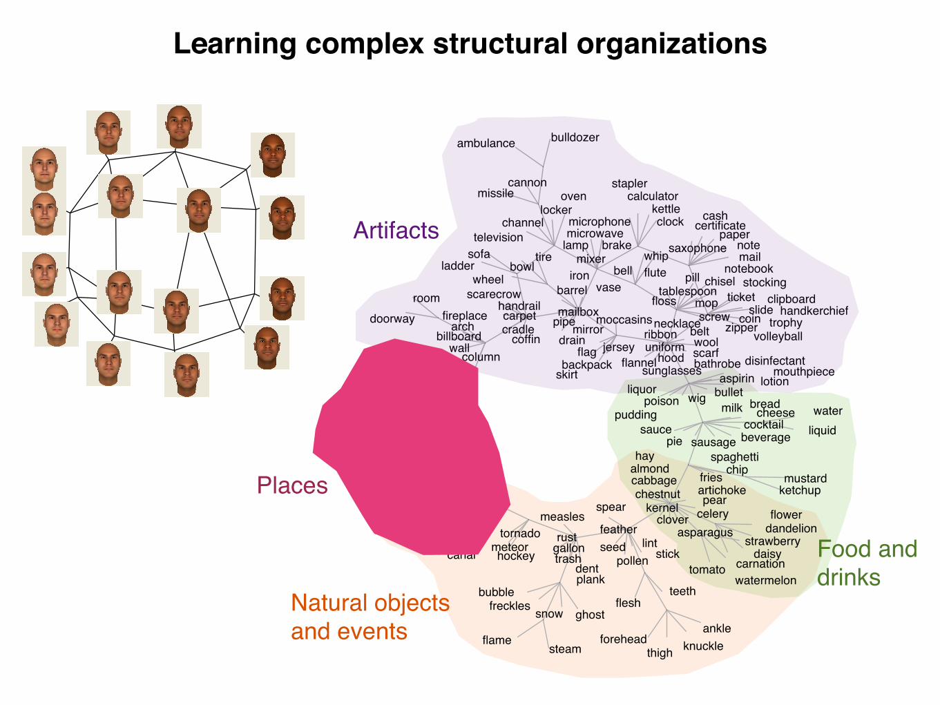
Artifacts
forest
mouthpiece
boy
asparagus
cannon
celery
coin
flag
brake
sausage
plank
farm
lambrattlesnake
salmon
liquor
hyena
museum
ketchupspear
microwave
flute
hay
ticket
meteor
doorway
spaghetti
belt
flower
flame
carnation
tornado
sunglasses
ghost
bullet
artichoke
scarfdrain
oak
slide
bathrobe
snow
arch
freckles
television
ribbon
clipboard
flesh
bay
fries
forehead
wall
lion
oven
lintdandelion
elephant
tire
stadium
leopard
necklace
bubble
watermelon
steam
backpack
ladderwhip
water
jersey
rust
trash
chip
calf
bell
bulldozer
trophy
beverage
tomato
certificate rabbitlocker dolphin
teeth
measles
tablespoon
clock
zippermirror
dinosaurstapler
stick
missile
feather
aspirinwig
pipe
fly
cocktail
buffalo
octopus
tigerchannel
chisel
paper
pond
fireplace
skirt
pet
handrail
calculator
uniform
mop
glacier
daisy
cradlebillboard
crocodile
trout
ankle
rhinoceros
person
disinfectant
floss
clover
village
coffin
donkey
lotion
roomstockingiron
kettle
pig
column
mustard
carpet
rainstorm
pill
saucepie
barrel
milk
kernel
thigh
hood
sofa
wool
puddingdock
gorilla
wheel
hut
jail
ambulance
strawberry
haddock
pollen
peacock
saxophone note
liquid
screw
canal
walrus
mixer
microphone
handkerchief
flannel
hen
mailbox
bowl
salamander
meadow
volleyball
scarecrow
cabbage
moccasins
vase
dent
poison
gallon
bedroombuilding
world pear
bread
basement
cash
notebook
chestnut
knuckle
almond
wolf
hockey
lamp
seed
cheesestable
sewerPlaces
Natural objects and events
Food and drinks
1
2
3
4
5
6
7
8
9
1011
12
13
1415
16
Learning complex structural organizations
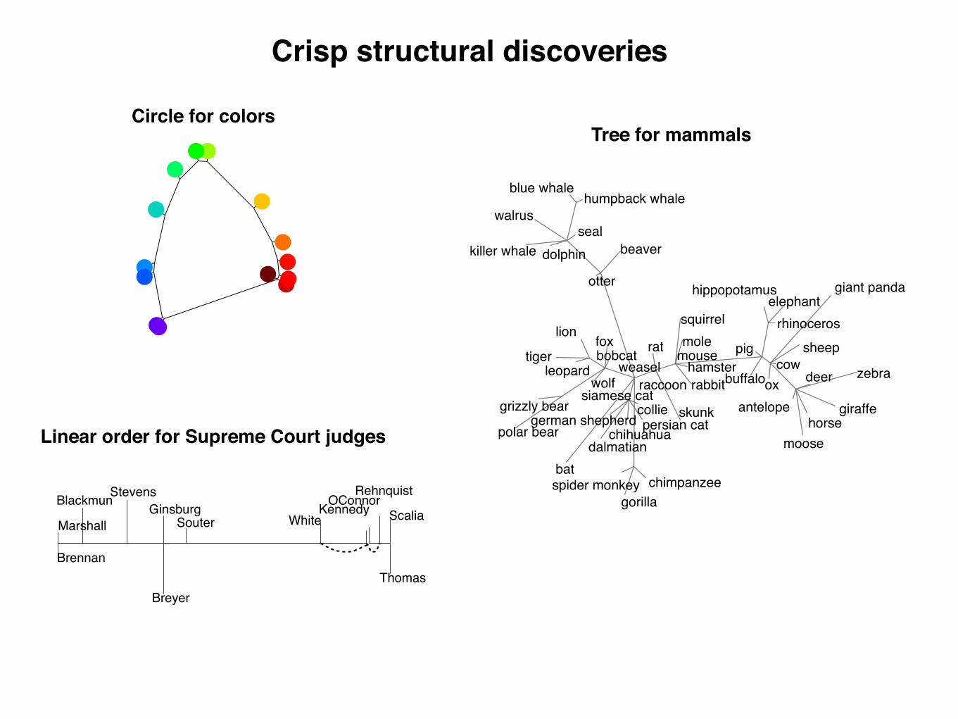
antelope
grizzly bear
killer whale
beaver
dalmatian
persian cat
horse
german shepherd
blue whale
siamese cat
skunk
mole
tiger
hippopotamus
leopard
moose
spider monkeyhumpback whale
elephant
gorilla
ox
fox
sheep
seal
chimpanzee
hamster
squirrel
rhinoceros
rabbitbat giraffe
wolf
chihuahua
ratweasel
otter
buffalo
zebra
giant panda
deer
bobcat
pig
lion mousepolar bear
collie
walrus
raccoon
cow
dolphin
gorilla
bat
giraffe
otter
cow
antelope
grizzly bear
killer whale
beaver
dalmatian
persian cathorse
german shepherd
blue whale
siamese cat
skunkmole
tiger
hippopotamus
leopard
moose
spider monkey
humpback whale
elephant
ox
fox
sheep
seal
chimpanzee
hamstersquirrel
rhinocerosrabbit
wolf
chihuahua
ratweasel
buffalozebra
giant pandadeerbobcat
pig
lion
mouse
polar bear
collie
walrus
raccoon
dolphin
A B
C D
antelope
grizzly bear
killer whale
beaver
dalmatianpersian cat
horse
german shepherd
blue whale
siamese cat
skunk
mole
tiger
hippopotamus
leopard
moose
spider monkey
humpback whale
elephant
gorilla
ox
fox
sheep
seal
chimpanzee
hamstersquirrel
rhinoceros
rabbit
bat
giraffe
wolf
chihuahua
ratweasel
otter
buffalo
zebragiant panda
deer
bobcat
pig
lion
mousepolar bearcollie
walrus
raccoon
cow
dolphin
antelopegrizzly bear
killer whale beaver
dalmatianpersian cat horsegerman shepherd
blue whale
siamese catskunk
moletiger
hippopotamus
leopard
moose
spider monkey
humpback whale
elephant
gorilla
ox
fox sheep
seal
chimpanzee
hamster
squirrel rhinoceros
rabbit
bat
giraffe
wolf
chihuahua
ratweasel
otter
buffalo zebra
giant panda
deerbobcat pig
lionmouse
polar bearcollie
walrus
raccooncow
dolphin
Figure 7: Learned structures to represent the mammals data set. Structural sparsity with � = 8(A), tree-based structural form (B), 2D spatial structural form (C), and structural sparsity with� = 1 (D). Stronger edges are displayed as shorter.
� Osherson Osherson Minneapolis Houston Allhorse mammals cities
1 0.94 0.87 0.70 0.59 0.712 0.95 0.86 0.70 0.58 0.714 0.93 0.84 0.70 0.61 0.716 0.91 0.89 0.69 0.51 0.688 0.89 0.91 0.69 0.51 0.68
Table 3: Correlations between how people and the structural sparsity model judge inductivestrength, for several tasks concerning mammals and cities. Rows of the table indicate di↵erentvalues of the sparsity parameter �.
21
Marshall
Brennan
WhiteBlackmun
RehnquistStevens OConnorScaliaKennedy
Souter
Thomas
Ginsburg
Breyer
Linear order for Supreme Court judges
Circle for colorsTree for mammals
Crisp structural discoveries
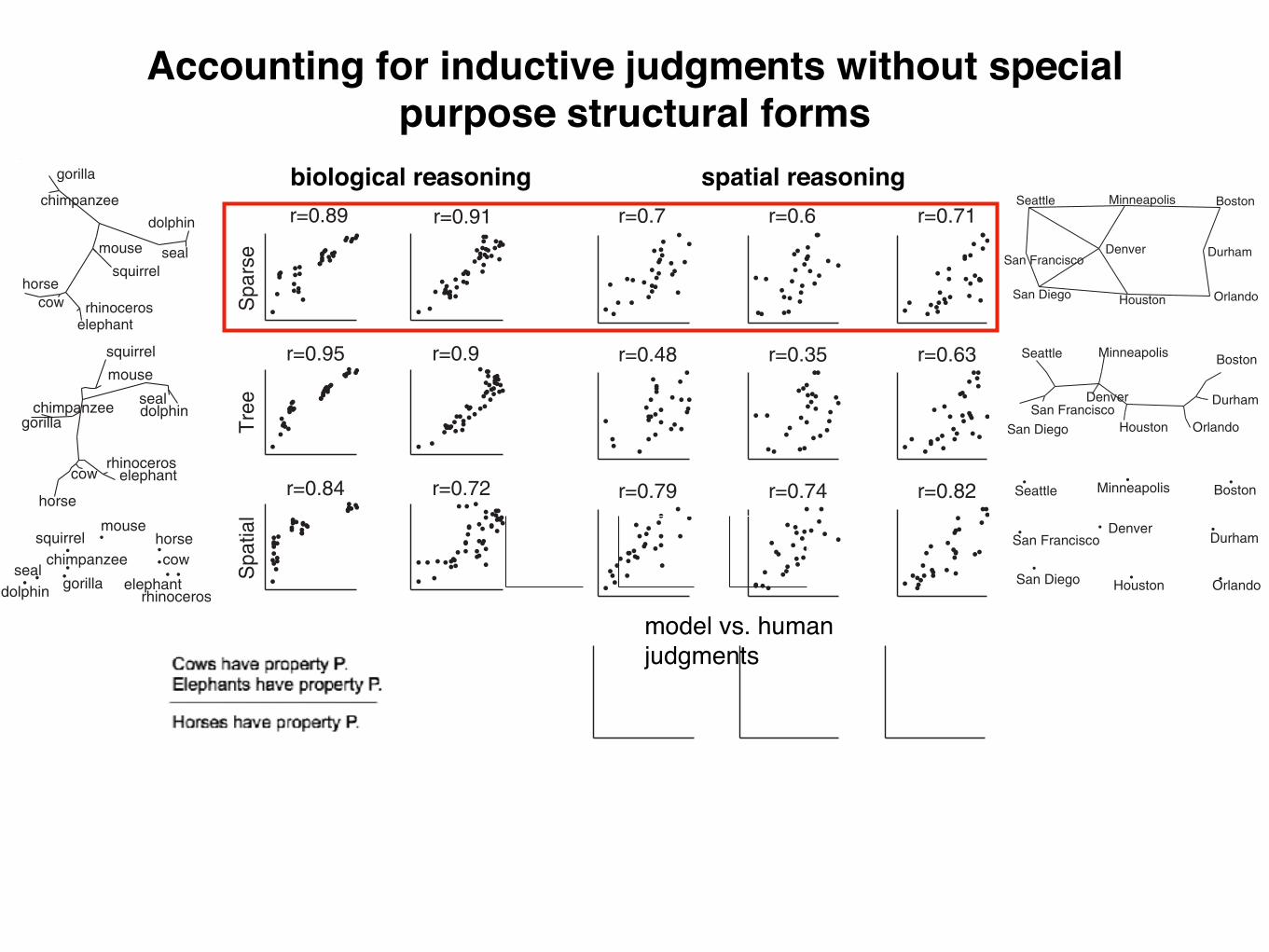
Σ, using distances in a 2D space
Rij ¼1
2pexpð# 1
rjjxi # xjjjÞ; ð4Þ
where xi is the 2D location of object i and ||xi # xj|| is the Euclidean distancebetween two objects.
• Raw covariance. The raw covariance model was either identical to the similaritymatrix or R ¼ 1
mDDT where D is the rescaled feature matrix.
5.3. Data sets for property induction
The property induction data concerning mammals, including the Osherson horse andOsherson mammals tasks, were reported in Osherson et al. (1990). Judgments concerned10 species: horse, cow, chimp, gorilla, mouse, squirrel, dolphin, seal, and rhino. Partici-pants were shown arguments of the form “Cows and chimps require biotin for hemoglo-bin synthesis. Therefore, horses require biotin for hemoglobin synthesis.” The Oshersonhorse set contains 36 two-premise arguments with the conclusion “horse,” and themammals set contains 45 three-premise arguments with the conclusion “all mammals.”Participants ranked each set of arguments in increasing strength by sorting cards.
Denver
Houston
Minneapolis
San Diego
San Francisco
Seattle
horse
elephantgorillaseal
chimpanzeesquirrel
mouse
cow
dolphin
horse
elephant
gorilla
sealchimpanzee
squirrel
rhinoceros
mouse
cow
dolphinDenver
Minneapolis
San DiegoSan Francisco
Seattle
Denver
Houston
Minneapolis
Durham
San Diego
San Francisco
Seattleiv) iv) i)
ii)
iii)
horse
elephant
gorilla
seal
chimpanzee
squirrel
rhinoceros
mouse
cow
dolphin
r=0.7 r=0.6 r=0.71
r=0.48 r=0.35 r=0.63
r=0.79 r=0.74 r=0.82
r=0.89 r=0.81 r=0.86
r=0.89
Spa
rse
r=0.91
r=0.95
Tre
e
r=0.9
r=0.84
Spa
tial
r=0.72
r=0.81
Osherson
Raw
r=0.8
Osherson
i)
ii)
iii)
(A) (B)
Boston
Durham
Boston
Houston Orlando
Durham
Boston
Orlando
rhinoceros Minneapolis Houston All citieshorse mammals Orlando
Fig. 6. Comparing models and human responses regarding property induction for mammals (A) and cities(B). A dot in (iv) is an inductive argument; for instance, the bottom-left dot for the “Osherson horse” dataset is the argument “dolphins and seals have this property, therefore horses do.” Each dot represents a differ-ent set of premises, followed by the conclusion category labeled on the x-axis (horse, all mammals, Min-neapolis, Houston, or all cities). Argument strength for the models (x-axis) is plotted against mean rank ofstrength across participants (y-axis), with the correlation coefficient r shown above. Predictions were com-pared for different types of structures, including those learned with structural sparsity (i), trees (ii), and 2Dspaces (iii). The arguments about mammals mention only the 10 mammals shown in (A), although predictionswere made by using the full structures learned for 50 mammals. Here only the subtrees (or space) that con-tains the pairwise paths between these 10 mammals are shown.
B. M. Lake, N. D. Lawrence, J. B. Tenenbaum / Cognitive Science (2018) 15
Σ, using distances in a 2D space
Rij ¼1
2pexpð# 1
rjjxi # xjjjÞ; ð4Þ
where xi is the 2D location of object i and ||xi # xj|| is the Euclidean distancebetween two objects.
• Raw covariance. The raw covariance model was either identical to the similaritymatrix or R ¼ 1
mDDT where D is the rescaled feature matrix.
5.3. Data sets for property induction
The property induction data concerning mammals, including the Osherson horse andOsherson mammals tasks, were reported in Osherson et al. (1990). Judgments concerned10 species: horse, cow, chimp, gorilla, mouse, squirrel, dolphin, seal, and rhino. Partici-pants were shown arguments of the form “Cows and chimps require biotin for hemoglo-bin synthesis. Therefore, horses require biotin for hemoglobin synthesis.” The Oshersonhorse set contains 36 two-premise arguments with the conclusion “horse,” and themammals set contains 45 three-premise arguments with the conclusion “all mammals.”Participants ranked each set of arguments in increasing strength by sorting cards.
Denver
Houston
Minneapolis
San Diego
San Francisco
Seattle
horse
elephantgorillaseal
chimpanzeesquirrel
mouse
cow
dolphin
horse
elephant
gorilla
sealchimpanzee
squirrel
rhinoceros
mouse
cow
dolphinDenver
Minneapolis
San DiegoSan Francisco
Seattle
Denver
Houston
Minneapolis
Durham
San Diego
San Francisco
Seattleiv) iv) i)
ii)
iii)
horse
elephant
gorilla
seal
chimpanzee
squirrel
rhinoceros
mouse
cow
dolphin
r=0.7 r=0.6 r=0.71
r=0.48 r=0.35 r=0.63
r=0.79 r=0.74 r=0.82
r=0.89 r=0.81 r=0.86
r=0.89S
pars
er=0.91
r=0.95
Tre
e
r=0.9
r=0.84
Spa
tial
r=0.72
r=0.81
Osherson
Raw
r=0.8
Osherson
i)
ii)
iii)
(A) (B)
Boston
Durham
Boston
Houston Orlando
Durham
Boston
Orlando
rhinoceros Minneapolis Houston All citieshorse mammals Orlando
Fig. 6. Comparing models and human responses regarding property induction for mammals (A) and cities(B). A dot in (iv) is an inductive argument; for instance, the bottom-left dot for the “Osherson horse” dataset is the argument “dolphins and seals have this property, therefore horses do.” Each dot represents a differ-ent set of premises, followed by the conclusion category labeled on the x-axis (horse, all mammals, Min-neapolis, Houston, or all cities). Argument strength for the models (x-axis) is plotted against mean rank ofstrength across participants (y-axis), with the correlation coefficient r shown above. Predictions were com-pared for different types of structures, including those learned with structural sparsity (i), trees (ii), and 2Dspaces (iii). The arguments about mammals mention only the 10 mammals shown in (A), although predictionswere made by using the full structures learned for 50 mammals. Here only the subtrees (or space) that con-tains the pairwise paths between these 10 mammals are shown.
B. M. Lake, N. D. Lawrence, J. B. Tenenbaum / Cognitive Science (2018) 15
Σ, using distances in a 2D space
Rij ¼1
2pexpð# 1
rjjxi # xjjjÞ; ð4Þ
where xi is the 2D location of object i and ||xi # xj|| is the Euclidean distancebetween two objects.
• Raw covariance. The raw covariance model was either identical to the similaritymatrix or R ¼ 1
mDDT where D is the rescaled feature matrix.
5.3. Data sets for property induction
The property induction data concerning mammals, including the Osherson horse andOsherson mammals tasks, were reported in Osherson et al. (1990). Judgments concerned10 species: horse, cow, chimp, gorilla, mouse, squirrel, dolphin, seal, and rhino. Partici-pants were shown arguments of the form “Cows and chimps require biotin for hemoglo-bin synthesis. Therefore, horses require biotin for hemoglobin synthesis.” The Oshersonhorse set contains 36 two-premise arguments with the conclusion “horse,” and themammals set contains 45 three-premise arguments with the conclusion “all mammals.”Participants ranked each set of arguments in increasing strength by sorting cards.
Denver
Houston
Minneapolis
San Diego
San Francisco
Seattle
horse
elephantgorillaseal
chimpanzeesquirrel
mouse
cow
dolphin
horse
elephant
gorilla
sealchimpanzee
squirrel
rhinoceros
mouse
cow
dolphinDenver
Minneapolis
San DiegoSan Francisco
Seattle
Denver
Houston
Minneapolis
Durham
San Diego
San Francisco
Seattleiv) iv) i)
ii)
iii)
horse
elephant
gorilla
seal
chimpanzee
squirrel
rhinoceros
mouse
cow
dolphin
r=0.7 r=0.6 r=0.71
r=0.48 r=0.35 r=0.63
r=0.79 r=0.74 r=0.82
r=0.89 r=0.81 r=0.86
r=0.89
Spa
rse
r=0.91
r=0.95
Tre
e
r=0.9
r=0.84
Spa
tial
r=0.72
r=0.81
Osherson
Raw
r=0.8
Osherson
i)
ii)
iii)
(A) (B)
Boston
Durham
Boston
Houston Orlando
Durham
Boston
Orlando
rhinoceros Minneapolis Houston All citieshorse mammals Orlando
Fig. 6. Comparing models and human responses regarding property induction for mammals (A) and cities(B). A dot in (iv) is an inductive argument; for instance, the bottom-left dot for the “Osherson horse” dataset is the argument “dolphins and seals have this property, therefore horses do.” Each dot represents a differ-ent set of premises, followed by the conclusion category labeled on the x-axis (horse, all mammals, Min-neapolis, Houston, or all cities). Argument strength for the models (x-axis) is plotted against mean rank ofstrength across participants (y-axis), with the correlation coefficient r shown above. Predictions were com-pared for different types of structures, including those learned with structural sparsity (i), trees (ii), and 2Dspaces (iii). The arguments about mammals mention only the 10 mammals shown in (A), although predictionswere made by using the full structures learned for 50 mammals. Here only the subtrees (or space) that con-tains the pairwise paths between these 10 mammals are shown.
B. M. Lake, N. D. Lawrence, J. B. Tenenbaum / Cognitive Science (2018) 15Accounting for inductive judgments without special purpose structural forms
spatial reasoningbiological reasoning
model vs. human judgments
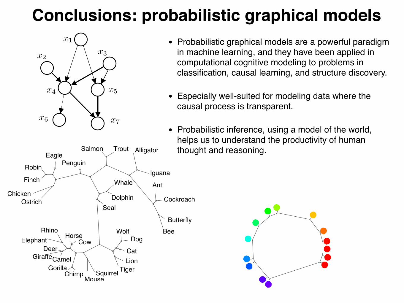
Conclusions: probabilistic graphical models• Probabilistic graphical models are a powerful paradigm
in machine learning, and they have been applied in computational cognitive modeling to problems in classification, causal learning, and structure discovery.
• Especially well-suited for modeling data where the causal process is transparent.
• Probabilistic inference, using a model of the world, helps us to understand the productivity of human thought and reasoning.
extent to which graphs with many clusters are penalized, and isfixed for all of our experiments. The normalizing constant forP(S!F) depends on the number of structures compatible with agiven form, and ensures that simpler forms are preferred when-
ever possible. For example, any chain Sc is a special case of a grid,but P(Sc!F ! chain) " P(Sc!F ! grid) because there are morepossible grids than chains given a fixed number of entities. Itfollows that P(Sc, F ! chain!D) " P(Sc, F ! grid!D) for any
NewYork
Bombay
Buenos Aires
Moscow
Sao Paulo
Mexico City
Jakarta
Tokyo
Lima
London
Bangkok
SantiagoLos Angeles
Berlin
Madrid
ChicagoVancouverToronto
Sydney
Perth
Anchorage
Cape Town
Nairobi
Vladivostok
Dakar
Kinshasa
Bogota
Honolulu
Wellington
CairoShanghai
Teheran
Irkutsk
Manila
Budapest
GinsburgBrennanScalia
Thomas
O'Connor
Kennedy
WhiteSouter
BreyerMarshallBlackmun Stevens Rehnquist
B
C
ElephantRhino Horse
Cow
CamelGiraffe
ChimpGorilla
MouseSquirrel Tiger
LionCat
DogWolf
SealDolphin
RobinEagle
Chicken
Salmon Trout
Bee
Iguana
Alligator
Butterfly
AntFinch
Penguin
Cockroach
Whale
Ostrich
Deer
E
A
D
Fig. 3. Structures learned from biological features (A), Supreme Court votes (B), judgments of the similarity between pure color wavelengths (C), Euclideandistances between faces represented as pixel vectors (D), and distances between world cities (E). For A–C, the edge lengths represent maximum a posteriori edgelengths under our generative model.
4
3
5
21
WolfowitzRicePowellAshcroftCheneyCard
1
Bush
MyersFeith
Armitage
Libby
DC
Whitman
Rumsfeld
111 321
23
A
P CAB R WL CABRMWRP
WFMR
6
CLCW
A
F
A B
Fig. 4. Structures learned from relational data (Upper) and the raw data organized according to these structures (Lower). (A) Dominance relationships among a troopof sooty mangabeys. The sorted data matrix has most of its entries above the diagonal, indicating that animals tend to dominate only the animals below them in theorder. (B) A hierarchy representing interactions between members of the Bush administration. (C) Social cliques representing friendship relations between prisoners.The sorted matrix has most of its entries along the diagonal, indicating that prisoners tend only to be friends with prisoners in the same cluster. (D) The Kula ringrepresenting armshell trade between New Guinea communities. The relative positions of the communities correspond approximately to their geographic locations.
Kemp and Tenenbaum PNAS ! August 5, 2008 ! vol. 105 ! no. 31 ! 10689
COM
PUTE
RSC
IEN
CES
PSYC
HOLO
GY
SEE
COM
MEN
TARY
x1
x2x3
x4 x5
x6 x7
extent to which graphs with many clusters are penalized, and isfixed for all of our experiments. The normalizing constant forP(S!F) depends on the number of structures compatible with agiven form, and ensures that simpler forms are preferred when-
ever possible. For example, any chain Sc is a special case of a grid,but P(Sc!F ! chain) " P(Sc!F ! grid) because there are morepossible grids than chains given a fixed number of entities. Itfollows that P(Sc, F ! chain!D) " P(Sc, F ! grid!D) for any
NewYork
Bombay
Buenos Aires
Moscow
Sao Paulo
Mexico City
Jakarta
Tokyo
Lima
London
Bangkok
SantiagoLos Angeles
Berlin
Madrid
ChicagoVancouverToronto
Sydney
Perth
Anchorage
Cape Town
Nairobi
Vladivostok
Dakar
Kinshasa
Bogota
Honolulu
Wellington
CairoShanghai
Teheran
Irkutsk
Manila
Budapest
GinsburgBrennanScalia
Thomas
O'Connor
Kennedy
WhiteSouter
BreyerMarshallBlackmun Stevens Rehnquist
B
C
ElephantRhino Horse
Cow
CamelGiraffe
ChimpGorilla
MouseSquirrel Tiger
LionCat
DogWolf
SealDolphin
RobinEagle
Chicken
Salmon Trout
Bee
Iguana
Alligator
Butterfly
AntFinch
Penguin
Cockroach
Whale
Ostrich
Deer
E
A
D
Fig. 3. Structures learned from biological features (A), Supreme Court votes (B), judgments of the similarity between pure color wavelengths (C), Euclideandistances between faces represented as pixel vectors (D), and distances between world cities (E). For A–C, the edge lengths represent maximum a posteriori edgelengths under our generative model.
4
3
5
21
WolfowitzRicePowellAshcroftCheneyCard
1
Bush
MyersFeith
Armitage
Libby
DC
Whitman
Rumsfeld
111 321
23
A
P CAB R WL CABRMWRP
WFMR
6
CLCW
A
F
A B
Fig. 4. Structures learned from relational data (Upper) and the raw data organized according to these structures (Lower). (A) Dominance relationships among a troopof sooty mangabeys. The sorted data matrix has most of its entries above the diagonal, indicating that animals tend to dominate only the animals below them in theorder. (B) A hierarchy representing interactions between members of the Bush administration. (C) Social cliques representing friendship relations between prisoners.The sorted matrix has most of its entries along the diagonal, indicating that prisoners tend only to be friends with prisoners in the same cluster. (D) The Kula ringrepresenting armshell trade between New Guinea communities. The relative positions of the communities correspond approximately to their geographic locations.
Kemp and Tenenbaum PNAS ! August 5, 2008 ! vol. 105 ! no. 31 ! 10689
COM
PUTE
RSC
IEN
CES
PSYC
HOLO
GY
SEE
COM
MEN
TARY
Excellent textbook for deeper reading


