
Propensity Score Adjustment for UnmeasuredConfounding in Observational Studies
Lawrence C. McCandless
Sylvia Richardson
Nicky G. Best
Department of Epidemiology and Public Health, Imperial College London, UK.
Version of March 2008
Corresponding author:
Lawrence McCandlessResearch Associate in BiostatisticsDepartment of Epidemiology and Public HealthFaculty of MedicineImperial College LondonNorfolk PlaceLondon UK W2 [email protected]: 077 9545 7264www.imperial.ac.uk/medicine/people/l.mccandless/
1

Abstract
Adjusting for several unmeasured confounders is a challenging problem in the analysis of obser-
vational data. Information about unmeasured confounders is sometimes available from external
validation data, such as surveys or secondary samples drawn from the same source population.
In principal, the validation permits us to recover information about the missing data, but the
difficulty is in eliciting a valid model for nuisance distribution of the unmeasured confounders.
Motivated by a British study of the effects of trihalomethane exposure on full-term low birth-
weight, we describe a flexible Bayesian procedure for adjusting for a vector of unmeasured
confounders using external validation data. We summarize the unmeasured confounders with a
scalar summary score using the propensity score methodology of Rosenbaum and Rubin. The
score has the property that it breaks the dependence between the exposure and unmeasured
confounders within levels of measured confounders. To adjust for unmeasured confounding in a
Bayesian analysis, we need only update and adjust for the summary score during Markov chain
Monte Carlo simulation. We demonstrate that trihalomethane exposure is associated with in-
creased risk of full-term low birthweight, and this association persists even after adjusting for
eight unmeasured confounders. Empirical results from simulation illustrate that our proposed
method eliminates bias from several unmeasured confounders, even in small samples.
Keywords: Confounding; Bias; Observational studies; propensity scores, causal inference
Running title: Adjustment for Unmeasured Confounders.
2

1. Introduction
Statistical methods for adjusting for unmeasured confounding in observational studies have been
studied extensively in recent years [1–6]. A popular strategy is to work from the assumption that
there is a single binary unmeasured confounder. In regression analysis, this gives a parametric
model for the observed data, averaging over the distribution of the unmeasured confounder. The
resulting model is nonidentifiable and indexed by so-called bias parameters that characteristic
the confounding effect of the missing covariate. To adjust for unmeasured confounding, the
investigator uses sensitivity analysis and computes inferences over a range of possible values for
the bias parameters. A Bayesian approach is also possible where uncertainty about bias param-
eters is incorporated into the analysis as prior information [1, 7, 8]. The posterior distribution
for the exposure effect summarizes uncertainty from unmeasured confounding in addition to
random error.
In practice we may have complicated patterns of missing confounders, and the assumption
of a binary unmeasured confounder may be simplistic. One estimation strategy is to model the
unmeasured confounders as missing data within a Bayesian framework [1, 9]. We model the joint
distribution of the data and unmeasured confounders. Inference proceed via posterior updating
of the unmeasured confounders using Markov chain Monte Carlo (MCMC) in a manner akin to
multiple imputation. But the difficulty with this approach is in eliciting a satisfactory model
for the distribution of the unmeasured confounders. They may be high dimensional, correlated
and either continuous or categorical. Parametric models may give inadequate representations
of complex patterns of missing data.
In this article, we consider the case where supplementary information on unmeasured con-
founding is available from external validation data. Examples include survey data or secondary
3

samples from the population under study. Thus our setting is observational studies where there
is bias from missing data, which we alleviate by synthesising different sources of empirical ev-
idence. We distinguish between the primary data which denotes the original dataset and the
validation data which denotes a smaller sample of units drawn from the same source population
and with complete information about missing variables. The motivation for this work is the
intuitive idea that it should be possible to develop a flexible procedure for using the validation
data in order to recover information about the confounding effect of missing covariates.
The problem of combining inference for primary and validation data for control of unmea-
sured confounding has been studied in the context of two-stage sampling designs. Schill et
al. [10], Breslow et al. [11] review two stage sampling methods for control of confounding
and other biases in observational studies. Fully parametric methods for adjusting for multiple
unmeasured confounders from validation data are available [12–16]. These approaches can be
somewhat restrictive because they require that the unmeasured confounders follow a specific
family of multivariate distributions. Alternatively, Chatterjee et al. [17] reviews techniques
which use density estimates of the distribution of the unmeasured confounders in the validation
data. There is also a large literature on adjusting for missing covariates via design-based esti-
mators derived from estimating equations. These circumvent the need for a parametric model
for missing covariates by calculating inferences using sampling weights. See Schill et al. [10]
and Breslow et al. [11] for details.
In this article we describe a Bayesian method for adjusting for multiple unmeasured con-
founders using external validation data. We use the idea of propensity scores, originally in-
troduced by Rosenbaum and Rubin [18]. The method can be a used in settings where the
confounders are either continuous and categorical with correlated components. We summarize
4
the unmeasured confounders using a scalar summary score, which can be interpreted as the
propensity score adjusted for measured confounders. The score has the property that it breaks
the association between the exposure and unmeasured confounders, within levels of measured
confounders. To adjust for unmeasured confounding using Bayesian techniques, we need only up-
date and adjust for the summary score during Markov chain Monte Carlo simulation. Modelling
variation in the outcome variable within levels of the unmeasured confounders is unnecessary.
To illustrate the problem of unmeasured confounding, Section 2 begins by describing a large
epidemiological investigation of the effect of trihalomethanes, a water disinfection by-product, on
risk of low birthweight in England. The primary data are obtained from United Kingdom Birth
Registry which benefits from a large sample size but has only limited information on factors
influencing birthweight such as maternal smoking and ethnicity. Rich covariate information
on eight unmeasured confounders is taken from validation data from the Millennium cohort
study. In Section 3, we describe a method for adjusting for unmeasured confounding using
propensity score techniques. We outline the model, prior distributions and an algorithm for
posterior simulation. Technical details concerning the propensity score and confounder control
are given in the Appendix. We apply the method in Section 4 and show that trihalomethane
exposure is associated with increased risk of low birthweight even after adjusting unmeasured
confounding. Furthermore, uncertainty from unmeasured confounding accounts for nearly 30%
of the total posterior uncertainty of the exposure effect. A brief simulation study in Section 5
illustrates that interval estimates which ignore this uncertainty will give inferences which are
falsely precise. Section 6 concludes with a discussion.
2. Example: Estimating the Effect of Trihalomethanes on Low
5

Birth Weight
To illustrate the problem of unmeasured confounding, we consider the example of an ob-
servational study of the relationship between trihalomethanes, a water disinfection by-product,
and risk of full-term low birth weight in the United Kingdom [19]. Pregnant mothers are be
exposed to trihalomethanes in a variety of different ways including bathing, drinking water or
swimming. Published investigations of adverse birth outcomes related to trihalomethane ex-
posure have yielded contradictory findings with some studies reporting increased risk of low
birthweight, while others showing no association [19]. Low birth weight is rare and any in-
creased risk due with trihalomethane exposure it is likely to be small. Furthermore, exposure
assessment is prone to measurement error and published studies are often missing information
on important confounders []. These study characteristics are likely to mask any true association.
In the present investigation, we consider the data from a previous study by Toledano et
al. [19, 20]. Information was collected for 9060 births between 2000 and 2001 in the region of
North West England serviced by a single water utility company. Birth records from the United
Kingdom National Births Registry were linked to estimates of trihalomethane water concentra-
tions using maternal residence at birth. Following the terminology given in the introduction,
we call this dataset the primary data. The National Births Registry data have the advantage of
capturing information on all births in the population under study. But it contains only limited
information on mother and infant characteristics which may impact birth weight. Complete
details on the data are given by [19, 20].
Let Y be an indicator variable for the outcome under study, taking value one if an infant
has full term low birth weight, and zero otherwise. Full term low birthweight is defined as a
gestational age greater than 37 weeks in combination with a birthweight less than 2.5kg. In
6

this investigation, the quantity Y for each of the 9060 subjects is obtained is obtained from
the data and model of Molitor et al. [16] as a single imputation of the outcome variable. To
model exposure to trihalomethanes, we let X be an indicator variable taking value one for a
concentration greater than ≥ 60µmol/L and zero otherwise. Let C denote a vector of p = 5
confounding variables that are contained in the primary data. These include indicator variables
for mother’s age (≤ 20, 20-24, 25-29, 30-34, ≥ 35), and an indicator variable if the baby gender
is male.
To explore the association between X and Y in the primary data, we fit a logistic regression of
Y on X while adjusting for C. The results are presented in Table 1 under the heading “NAIVE”.
We see a an odds ratio of 2.27 with 95% CI (1.68, 3.06) indicating that trihalomethane exposure
is associated with a sizeable increase in risk of full term low birth weight.
A difficulty with this analysis is that the effect estimate is likely to be biased from unmeasured
confounding. Owing to the limited number of variables in the primary data, there is limited
information on factors that influence birth weight, including maternal smoking, ethnicity or
income. Trihalomethane concentrations may vary by neighbourhood income level. Without
appropriate adjustment for confounding, the risk patterns between exposure groups may be an
artifact of systematic differences in characteristics between populations.
In this investigation, information about unmeasured confounders is available from external
validation data. The United Kingdom Millennium Cohort Study [20] contains survey information
on mothers and infants born during the period 2000-2001 when the primary data were collected.
The data are a disproportionately stratified sample based on ethnicity and income of place of
residence. Following Molitor et al. [20] we link the survey data with that of the National Birth
Registry to obtain partial information about unmeasured confounders for 1115 out of a possible
7

9060 births. Thus the primary data have sample size m = 7945, while the validation data have
sample size m = 1115. We let U be a q = 8 vector of eight unmeasured confounders including;
indicator for lone parent family, number of live children for mother, maternal smoking, alcohol
consumption , body mass index prior to pregnancy, ethnicity (three categories), income (ordinal
with three levels calculated from tertiles in the population), and indicator variable for the mother
having high school diploma.
Denote the primary data as {(Yi, Xi, Ci, Ui)| for i ∈ 1 : m = 7945} and the validation data
as {(Yj, Xj, Cj, Uj)| for j ∈ 1 : m = 1115}. The quantity Ui is completely unobserved. To
study the impact of unmeasured confounding, Table 2 presents odds ratios for the association
between Yj and Xj when adjusting for Cj alone, versus adjusting for Cj and Uj. In the first
column of Table 2, we fit weighted logistic regression of Yj on Xj and Cj using the survey
weights supplied in the documentation of the validation data in order to correct for non-random
sampling. The odds ratio is equal to 2.52 with 95% CI (1.03, 6.15). In the second column we fit
the same regression, but adjust for both Cj and Uj and obtain 2.43 (0.95, 6.24). The exposure
effect estimates are similar, but the interval estimate in the fully adjusted analysis is wider and
crosses zero. Furthermore, smoking and ethnicity are important predictors of low birth weight.
Thus Table 2 indicates that the components of U play an important role in explaining
variation in the outcome. Valid inference from the primary data may require adjustment for
unmeasured confounding. As discussed in the introduction, a standard analytic approach is to
model the unmeasured confounders as missing data. But this is challenging because the com-
ponents of Uj are correlated binary variables which depend on Xj and possibly Cj. In Section
3, we present Bayesian procedure for summarizing and adjusting for the confounding effect of
Ui using propensity scores.
8

3. Bayesian Adjustment for Unmeasured Confounding (BAYES).
We present a method for Bayesian adjustment for unmeasured confounding using external
validation data, which we henceforth call by the acronym BAYES. The BAYES method uses
the idea of propensity scores, described by Rosenbaum and Rubin [18], in order to build a scalar
summary of Ui which is included as a covariate in a regression model for the outcome. In Sec-
tion 3.1 that follows, we describe a model for unmeasured confounding. We model the density
function P (Y,X, U |C) and integrate over the unmeasured U . This gives likelihood functions for
the primary data and validation data that can be used for Bayesian inference. A family of prior
distributions for model parameters is given in Section 3.2. Section 3.3 describes an algorithm for
sampling from the posterior distribution using MCMC. This permits us to calculate estimates
of the exposure effect which adjusts unmeasured confounders.
3.1 Models
3.1.1 A Model When There Is No Unmeasured Confounding
Suppose that (Yi, Xi, Ci, Ui) and (Yj, Xj, Cj, Uj) for i ∈ 1 : n and j ∈ 1 : m are identically
distributed observations drawn from the same population with probability density function
P (Y,X, C, U). Building on the Bayesian propensity score analysis of McCandless et al [21], we
model the conditional density P (Y,X|C, U) using a pair of logistic regression models:
Logit[P (Y = 1|X, C, U)] = βX + ξT C + ξT g{Z(U)} (1)
Logit[P (X = 1|C, U)] = γT C + Z(U), (2)
where Z(U) = γT U .
Equation (1) is a model for the outcome and includes a exposure effect parameter β and a
linear term for the covariates C with regression coefficients ξ = (ξ0, . . . , ξp). Equation (2) models
9

the probability of exposure, which depends on the measured and unmeasured confounders via
the regression coefficients γ = (γ0, . . . , γp) and γ = (γ1, . . . , γq). To ease modelling of regression
intercept terms, we set the first component of C equal to one, so that C is a (p + 1)× 1 vector.
In equations (1) and (2), the quantity Z(U) = γT U is a scalar summary of U , which can
be interpreted as the propensity score adjusted for C. To illustrate, the propensity score on
the log odds scale is defined as Logit[P (X = 1|C, U)], according to the original definition of
Rosenbaum and Rubin [18]. From equation (2), this quantity follows a regression model and is
given by γT C + γT U . If we condition on C, then quantity γT C is a constant intercept term. In
the Appendix, we prove that Z(U) has the property that
X ⊥⊥ U |C, Z(U). (3)
This result is analogous to Theorem 1 of Rosenbaum and Rubin [18]. It says that within levels
of C, conditioning on Z(U) forces independence between X and U . Variability in X due to U
is mediated entirely through Z(U). The summary score Z(U) breaks the association between
the unmeasured confounders and exposure.
In Theorem 2 of the Appendix, we prove that if there is no unmeasured confounding condi-
tional on (C, U), then equation (3) implies that there is no unmeasured confounding conditional
on (C, Z(U)). This means that exposure effect measures computed from the marginal density
P (Y |X, C, Z(U)) have a causal interpretation. To control for confounding bias due to U , it
suffices to stratify on (C, Z(U)). We can estimate the exposure effect by using models which
assume that Y ⊥⊥ U |X, C, Z(U).
Accordingly, equation (1) includes the quantity Z(U) as a covariate in a regression model
for the outcome via a linear predictor g{.}. For the trihalomethane data example, we let
g{a} =∑l
j=0 ξjgj{a} where the quantities gj{.} are natural cubic spline basis functions with
10

l = 3 knots (q1, q2, q3) and regression coefficients ξ = (ξ0, ξ1, ξ2, ξ3) [22]. This gives a smooth yet
flexible relationship between Z(U) and outcome within levels of X and C. The choice of l = 3
knots reflects a trade off between smoothness and complexity. See Austin and Mamdani [22]
for a detailed discussion of regression modelling strategies which use the propensity score as a
regression covariate.
We could alternatively control confounding from C and U by fitting the outcome model
Logit[P (Y = 1|X, C, U)] = βX + ξT g{Z(U,C)} (4)
where Z(U,C) = Logit[P (X = 1|U,C)] = γT C + γT U . This is a standard approach to control-
ling confounding, and it does not distinguish between measured and unmeasured confounders
in calculating the propensity score. However, an advantage of using equation (1) rather than
equation (4) is that it allows direct modelling of variability in Y arising from C. We include
a linear term “... + ξT C + ..” while summarizing the contribution of U using the Z(U). This
is appropriate in the present context because C is measured while U is not. Furthermore, the
summary score Z(U) has the appealing property that in the special case when γ = 0 in equation
(2), then Z(U) is equal to the log odds of the propensity score. In this case, U is the only
confounder for the effect of X on Y , and equation (1) reduces to standard regression adjustment
for the propensity score, as advocated by Rosenbaum and Rubin [18].
3.1.2 A Model for Unmeasured Confounding
In the primary data, the quantities Yi, Xi and Ci are observed in the registry data while Ui
is not. Equations (1) and (2) define the density P (Y,X|C, U), and we can use it to calculate
11

the marginal model for P (Y,X|C) integrating over U . We have
P (Y,X|C) = E{P (Y, U,X|C)}
=
∫P (Y |X, C, U)P (X|C, U)P (U |C)dU, (5)
where P (Y |X, C, U) and P (X|U,C) are given in equations (1) and (2). To complete the speci-
fication, we require a model for U given C.
One simplification is to assume that C and U are marginally independent, meaning that
P (U |C) = P (U). In this case, we can model P (U) using the empirical distribution of U1, . . . , Um
from the validation data alone. We may approximate
P (Y,X|C) ≈ 1
m
m∑j=1
P (Y |X, C, Uj)P (X|Uj, C). (6)
Using this approach, we model P (Y,X|C) = E{P (Y, U,X|C)} as the empirical average of
P (Y |X, C, Uj)P (X|Uj, C) over replicates Uj. An advantage of this representation is that it
requires no parametric model for the distribution of Uj. It can be used regardless of whether
the components of Uj are correlated and contain both continuous and categorical variables.
In practice, measured and unmeasured confounders are likely to be correlated, and the as-
sumption that P (U |C) = P (U) will be implausible. Because the components of U are categori-
cal in the trihalomethane data, it would be possible to assign a parametric model for P (U |C).
Nonetheless, previous authors have argued that ignoring these correlations leads to inferences
which are conservative under fairly general settings. Fewell et al. [23] study the impact of
confounding from multiple unmeasured variables using simulations. The authors show that
when measured and unmeasured variables are correlated this tends to reduced unmeasured con-
founding. Adjusting for measured variables has the secondary effect of partially adjusting for
unmeasured variables. This reasoning is also discussed by Schneeweiss [2].
12

In contrast to equation (5), previously proposed methods of sensitivity analysis for unmea-
sured confounding favour models of the form
P (Y |X, C) =
∫P (Y |X, C, U)P (U |X, C)dU,
which require models for P (U |X, C) [6–8, 24, 25]. The approach of equation (5) applies Bayes
rule to P (U |X, C) in order to switch the conditional dependence. The advantage is that the
model for P (X|C, U) comes “for free” in a propensity score analysis controlling for C and U .
Thus propensity score methods offer unique advantages in settings with unmeasured confound-
ing. Dimension reduction of covariates in regression modelling, simplifies missing data modelling
when some covariates are partially observed.
3.1.3 Bias Parameters and Nonidentifiability.
In equations (1) and (2), the parameters ξ, γ model the relationship between the unmeasured
confounder U and the data Y , X, C. We call these quantities bias parameters in the sense that
they model bias from unmeasured confounding. If the parameters γ or ξ are large in magnitude
then this means that U contains powerful confounders [26].
The model for the primary data given in equation (6) is nonidentifiable. To illustrate, suppose
that that validation data has sample size m = 1. Then equation (6) is becomes
P (Y,X|C) ≈
[exp(Y (βX + ξT C + ξT g{Z(U∗)}))1 + exp(βX + ξT C + ξT g{Z(U∗)})
] [exp(X(γT C + γT U∗}))1 + exp(γT C + γT U∗)
],
where U∗ is a known fixed quantity taken from the validation data. The conditional distribution
of Y given X and C cannot distinguish between the quantity ξ0 and ξT g{Z(U)} because they
both serve as regression intercept terms. We can only estimate the sum ξ0 + ξT g{Z(U)}. Simi-
larly, we cannot distinguish between γ0 and γT U . When U is unobserved, the density P (Y,X|C)
13

can arise from different and indistinguishable patters of unmeasured confounding and baseline
prevalences of Y and X.
If the bias parameters ξ and γ are known a priori, then the model for the primary data in
equation (6) is identifiable. The quantities ξT g{Z(U)} and γT U are known offsets in the density
P (Y,X|C). We can calculate the maximum likelihood estimate for (β, ξ, γ) from the likelihood
function for the primary data, given by
n∏i=1
P (Yi, Xi|Ci). (7)
Consequently, an alternative frequentist approach to adjusting for unmeasured confounding
would be to plug in estimates for the bias parameters ξ and γ into the model for P (Y,X|C)
in equation (6) and then maximize the resulting likelihood to estimate (β, ξ, γ). This approach
to external adjustment forms the basis of sensitivity analysis and is conceptually similar to the
procedure described by Rosenbaum and Rubin [3]. We revisit this maximum likelihood approach
in Section 4 and compare it to the BAYES method.
3.2 Prior Distributions
We assign proper independent normal priors to β, ξ, ξ, γ, γ.
α, β, ξ1, . . . , ξp, ξi, . . . , ξp, γ1, . . . , γp, γi, . . . , γp ∼ N
{0,
(log(15)
2
)}
The priors models the belief that the odds ratio for the exposure effect β is not overly large and
lies between 1/15 and 15 with probability 95%. Similarly, the priors make analagous modelling
assumptions about the prior magnitude for the association between Y and C, Z(U) given X,
and also the association between C, U and X.
14

3.3 Posterior Simulation
Let data denote the both the primary and validation data {(Yi, Xi, Ci); for n = 1 : n} and
{(Yi, Xi, Ci); for n = 1 : n and }, respectively. Inferences from BAYES are obtained from the
posterior density P (β, ξ, ξ, γ, γ|data), which we sample from using MCMC simulation techniques.
We have
P (β, ξ, ξ, γ, γ|data) ∝{ n∏
i=1
P (Yi, Xi|Ci)}×
{ m∏j=1
P (Yj, Xj|Cj, Uj)}
×P (β, ξ, ξ, γ, γ)
where the products over i and j are the likelihood functions for the primary and validation data,
respectively, and P (β, ξ, ξ, γ, γ) is the prior density for β, ξ, ξ, γ and γ.
We sample from P (α, β, ξ, ξ, γ, γ|data) by updating from the conditional distributions for
[β, ξ, ξ|γ, γ, data] and [γ, γ|β, ξ, ξ, data] using the Metropolis Hastings algorithm. To update
from [β, ξ, ξ|γ, γ, data], we use a proposal distribution based on a random walk which updates
each component β, ξ0, . . . , ξp, ξ1, . . . ξk one at a time using a mean zero normal disturbance.
Multivariate updating from [γ, γ|β, ξ, ξ, data] is accomplished using the algorithm described in
McCandless et al [21].
A difficulty with this sampling scheme is that the likelihood for the primary data is expensive
to compute. It requires calculating P (Yi, Xi|Ci, Uj) over all combinations of i and j. Alterna-
tively, we can recognise that the expression for P (Y,X|C) in (6) is a sample mean estimate of
E{P (Y, U,X|C)}. We can use a quadrature estimate
P (Y,X|C) =M∑
k=1
ωk
[exp{Y (βX + ξT C + ξT g{Zk})}1 + exp{βX + ξT C + ξT g{Zk}}
] [exp{X(γT C + Zk)}1 + exp{γT C + Zk}
](8)
based on a histogram of γT U1, . . . γT Um. The quantities Zk are the interval midpoints in the
histogram and ωk are the bin frequencies. In applications we find this summation much faster
15

to calculate compared to equation (6) because it requires far fewer evaluations of P (Y,X|C, U).
4. Analysis Results for the Trihalomethane Data
4.1 Bayesian Adjustment for Unmeasured Confounding (BAYES).
Before applying the BAYES method to the trihalomethane data, we set a priori values for
the knots used define the linear predictor g{.} in equation (1). Following McCandless et al
[21], we fit the logistic regression model given in equation (2) to the validation using maximum
likelihood to estimate the bias parameter γ. The estimated CPS, computed by evaluating
{γT Uj, for j ∈ 1 : m}, range from -0.1 to 2.0 with median equal 0.35 and interquartile range
(0.41, 0.67). Three knots are chosen as 0.41, 0.51 and 0.67 to define approximate quartiles for
the true distribution of the CPS.
We then apply BAYES to the data by sampling from the posterior density P (β, ξ, ξ, γ, γ|data).
As discussed in Section 2, the validation data in the Millennium Cohort Study are collected
through disproportionately stratified sampling, with survey weights supplied with the accompa-
nying documentation. We calculate the quantities in equations (6) and (8) by weighting the Uj
using the survey weights. We then obtain a single MCMC chain of length 100 000 after suitable
burn-in and thin the chain to retain 10 000 sample.
Figures 2 and 3 illustrate MCMC chains for model parameters and indicate that convergence
is not ideal. Interestingly, convergence of the parameters β, ξ, γ is much better than for the bias
parameters ξ and γ. These results are somewhat expected because the model for unmeasured
confounding is only weakly identifiable. As argued in Section 3.1.3, because U is unmeasured in
the primary data, there is little information to distinguish between the intercept ξ0 and linear
predictor ξT g{Z(U)}. Similarly, the MCMC sampler cannot distinguish between γ0 and γT U .
16

Sampler convergence problems are also reported in other contexts using non-identifiable models
[27, 28].
We argue that the mixing of β, ξ and γ is satisfactory for computing posterior summaries,
and that poor convergence of ξ and γ is not a serious concern. The reason is because the overall
model fit for the primary and validation data is unaffected by poor mixing. To illustrate, Figure
3 presents the mixing of the deviance, given by
−2 log
[n∏
i=1
P (Yi, Xi|Ci)
]×
[m∏
j=1
P (Yj, Xj|Cj, Uj)
],
calculated at each MCMC iteration. The deviance is a measure of overall model fit [9], with
low values correspond to better fitting. We see in Figure 3 that the deviance values are stable
across MCMC iterations. Poor convergence of the bias parameters has a modest impact on
model fit. Because the convergence the MCMC chain for β, ξ and γ is satisfactory, we can use
it to calculate valid posterior summaries.
Table 2 presents the results of the analysis under the heading “BAYES”, which contain
posterior means and 95% credible intervals for the exposure effect and covariate effects. We
see that adjustment for unmeasured confounding has a sizable impact on estimation of the
exposure effect. Trihalomethane exposure is associated with increased risk of low birthweight,
with odds ratio 1.96, 95% CI (1.32,2.92), and these inferences are robust to adjustment for eight
unmeasured confounders. The BAYES point estimate for β is shifted towards zero relative to
the NAIVE analysis which ignores unmeasured confounding. This results make sense because,
in Table 1, we see that when analyzing the validation data alone, adjustment for Cj and Uj
drives the estimate of β towards zero compared an analysis ignoring Uj.
The interval estimate for the exposure effect calculated from BAYES is longer than for
NAIVE, with length 1.60 versus 1.37. This result seems puzzling at first because an analysis of
17

the primary and validation data combined intuitively ought to yield less posterior uncertainty
compared to a NAIVE analysis of the primary data alone. Nonetheless, the NAIVE analysis
ignores bias uncertainty about unmeasured confounding. If there is bias in the registry data,
then the NAIVE interval estimates will be falsely precise without nominal 95% coverage lev-
els. McCandless et al. [21] investigate the frequentist performance of Bayesian credible interval
which model bias from unmeasured confounding.
4.2 Maximum Likelihood Estimation to Adjust for Unmeasured Con-
founding
For comparison, we also apply a method for adjusting for unmeasured confounding which
does not use Bayesian techniques. We call the method FREQ, meaning frequentist adjustment
for unmeasured confounding, and we define the method as follows. First, fit the regression
models in equations (1) and (2) in the validation data alone and compute maximum likelihood
estimates of the bias parameters ξ and γ. This is straightforward because Uj is observed.
Next, we substitute the point estimates into the likelihood function for the primary data, given
in equations (6) and (7), and maximize it with respect to (β, ξ, γ) using a Newton Raphson
algorithm. Estimated standard errors for are (β, ξ, γ) obtained from the observed information
matrix.
FREQ is as a fast analogue of BAYES. The validation data is used as a source of information
about bias parameter, but there is no simultaneous analysis of multiple datasets. There is no
propagation of uncertainty in the bias parameters through the analysis. We expect that interval
estimates for the exposure effect calculated from FREQ may be falsely precise. FREQ can also
be used as a diagnostic procedure to determine if BAYES is worthwhile. If FREQ and NAIVE
18

give markedly different inferences, then this indicates that unmeasured confounding is important
and BAYES is worthwhile. Both methods use the same knots (q1, q2, q3) in the linear predictor
g{.}.
The results of applying FREQ to the trihalomethane data are given in the third column of
Table 2. Comparing FREQ and BAYES, we can see that inferences are similar in the sense
that both estimates of the exposure effect are driven towards zero relative the NAIVE analysis.
Trihalomethane exposure is associated with risk of full term low birthweight. The association is
robust even after having adjusted for the eight unmeasured confounders in the validation data.
BAYES interval estimate for β are wider than for FREQ. Additionally, the FREQ interval
estimate for β has exactly the same length as the NAIVE estimate on the log odds scale. While
FREQ corrects for unmeasured confounding using the same models as BAYES, the method
ignores uncertainty in the bias parameters. It assumes that the bias parameters ξ and γ are
known exactly. In contrast, BAYES models and propagates uncertainty through the analysis.
This has a large impact on the length of interval estimates.
One strategy for reconciling the difference between BAYES and FREQ is to study the effect
of admitting uncertainty in the bias parameters the posterior variance of β. Using the relation
V ar[A] = E{V ar[A|B]}+ V ar{E[A|B]}, we can write
V ar[β] = E{V ar[β, ξ, γ|ξ, γ]}+ V ar{E[β, ξ, γ|ξ, γ]}, (9)
where expectations and variances are over posterior uncertainty in model parameters. This
gives an ANOVA type decomposition where the first term models uncertainty in β within bias
parameters, while the second term models uncertainty between bias parameters [29]. Denote
Vbetween = V ar{E[β, ξ, γ|ξ, γ]} and Vwithin = E{V ar[β, ξ, γ|ξ, γ]}. When the quantities ξ and
γ are known a priori, as is assume in FREQ, then Vbetween is equal to zero and the posterior
19
variance of β reduces to Vwithin. Conversely, when we admit uncertainty in the bias parameters,
then Vbetween is non-zero.
The ratio
Vbetween
Vbetween + Vwithin
models the proportion of uncertainty in β that is attributable to bias. As the sample size n
increase, the quantity Vwithin will tend to zero, while Vbetween remains constant. Thus the ratio
illustrates how bias uncertainty tends to dominate total uncertainty asymptotically in observa-
tional studies with bias from unmeasured confounding. Further discussion is given by Gustafson
[29]) and Greenland [1]. We can get a rough estimate of the ratio by comparing the width of
the 95% interval estimates for the exposure effect on the log odds scale. For BAYES the width
is 0.79 versus 0.60 for FREQ. Thus in the trihalomethane data, uncertainty from unmeasured
confounding accounts for nearly one third of the total posterior uncertainty for the exposure
effect. FREQ and NAIVE substantially under report the this uncertainty.
5. The Performance of BAYES and FREQ in Synthetic Data
The preceding analysis motivates questions about the performance of the BAYES in more
general settings. For example, is the scalar Z(U) from equation (1) an adequate summary
of U , giving unconfounded exposure effect estimates? Does modelling uncertainty in the bias
parameters give meaningful improvement in the coverage probability of interval estimates? A
further issue is the sample size m of the validation data. If m is small, then we might expect
that BAYES and FREQ will break down because they fail to recover the marginal distribution
of propensity scores in the source population. We explore these issues using simulations by
analyzing synthetic datasets which contain confounding from multiple unmeasured variables.
20
5.1 Simulation Design
We generate and analyze ensembles of 100 pairs of synthetic datasets, where each pair consists
of primary data with n = 1000 and validation data with m = 100, 250, 500 or 1000. We consider
the case where there are four measured confounders and four additional unmeasured confounders
(thus C is a 5× 1 vector and U is 4× 1). Primary data (n = 1000) and validation data (m =75,
100, 250, 500 and 1000) are generated using the following algorithm:
1. Simulate {Ci, Cj} for i ∈ 1 : n, j ∈ 1 : m, and also {Ui, Uj} for i ∈ 1 : n, j ∈ 1 : m, where
each component of Ci, Cj, Ui, Uj is independent and identically distributed as a N(0,1)
random variable.
2. For fixed γ0, . . . , γ4 = 0.1, and γ1, . . . , γ4 = 0.2, simulate {Xi, Xj} for i ∈ 1 : n, j ∈ 1 : m
for using the logistic regression model of equation (2).
3. For fixed β = 0, ξ0, . . . , ξ4 = 0.1 and ξ1, . . . , ξ4 = 0.2, simulate {Yi, Yj} for i ∈ 1 : n, j ∈ 1 :
m for using the model
Logit[P (Y = 1|X, C, U)] = βX + ξT C + ξT U.
Note that the first component of Ci and Cj is equal to one so that γ0 and ξ0 are regression
intercept terms.
We fix β = 0 to model the setting where there is no exposure effect. The choice for ξ, ξ, γ, γ
models moderate but realistic log odds ratios that are encountered in epidemiologic investigations
[30]. The bias parameters γ and ξ govern the association between the unmeasured confounder
and the treatment and outcome respectively. Setting γ and ξ to be large in magnitude induces
bias from unmeasured confounding.
21
We analyze the 100 pairs of datasets across for each combination of n and m using BAYES,
FREQ and NAIVE to obtain point and 80% interval estimates of the exposure effect β. Sampler
convergence is assessed using separate trial MCMC runs.
5.2 Results
Figure 4 summarizes the performance of BAYES, FREQ and NAIVE analyses of 100 syn-
thetic datasets. The upper three panels quantify bias and efficiency of point estimates for the
exposure effect β = 0, as a function of m the sample size in the validation data. The lower three
panels quantify coverage probability and average length of 80% interval estimates for β.
For the NAIVE analysis, estimates of β should perform poorly because the method ignores
unmeasured confounding. This is apparent in Figure 3. In the top right panel, the blue curve lies
far from zero indicating that NAIVE estimates are badly biased. The blue curve is flat and does
not depend on m because the NAIVE analysis ignores the validation completely. Similarly, in
the lower right panel, the blue curve hovers below 60%, indicating that the coverage probability
of NAIVE interval estimates is far below the nominal level of 80%.
In contrast, BAYES and FREQ eliminate unmeasured confounding over a wide range of
values for m. In the upper panels, we see that the blue curves hover near zero. BAYES and
FREQ are essentially unbiased for all m under consideration. Summarizing the four unmeasured
confounders using the summary score Z(U) appears to reduce confounding. We do not consider
the case where m < 100 corresponding to validation data which is less than 10% the size of the
primary data with n = 1000. The reason is because the validation data contain little information
about the bias parameters. The model for the primary data given in equation (6) is only weakly
identifiable. Sampler convergence deteriorates and point estimates of ξ, γ are highly variable.
22

There is little information available for adjustment for unmeasured confounding.
The lower panels of Figure 3 summarize the performance of interval estimates for the exposure
effect β. BAYES interval estimates have improved coverage probability compared to FREQ
or NAIVE. As m tends to zero, the coverage probability of FREQ drops off more sharply
compared to BAYES. Ignoring uncertainty in the bias parameters appears to adversely affects
interval estimation when the validation data is small. We note that the difference in coverage
estimates for BAYES versus FREQ is modest compared to the simulation standard errors.
However, reducing the standard errors by one half requires a fourfold increase in the number of
simulations, which is prohibitively expensive.
Somewhat surprisingly, inferences from BAYES may actually be more efficient than FREQ
or NAIVE. As expected, when the validation data is small BAYES interval estimates are wider.
This is consistent with intuition and the analysis of the trihalomethane data. Modelling un-
certainty in the bias parameters gives an increase in uncertainty in the exposure effect. But
for large m BAYES intervals are actually shorter than FREQ or NAIVE. Furthermore, BAYES
point estimates of β have smaller variance. Intuitively, the validation data contain information
about β which is ignored by FREQ. In equation (9), the quantity Vwithin tends to decrease
while the bias uncertainty Vbias increases. The resulting posterior variance for β is smaller than
the large sample variance from either FREQ or NAIVE. This reinforces the notion that a joint
analysis of the primary and validation data may be preferable. In Figure 3, there appears to
be little reason to choose FREQ over BAYES. When the validation data is small, FREQ will
under report uncertainty, and when the validation data is large FREQ will suffer on efficiency.
23
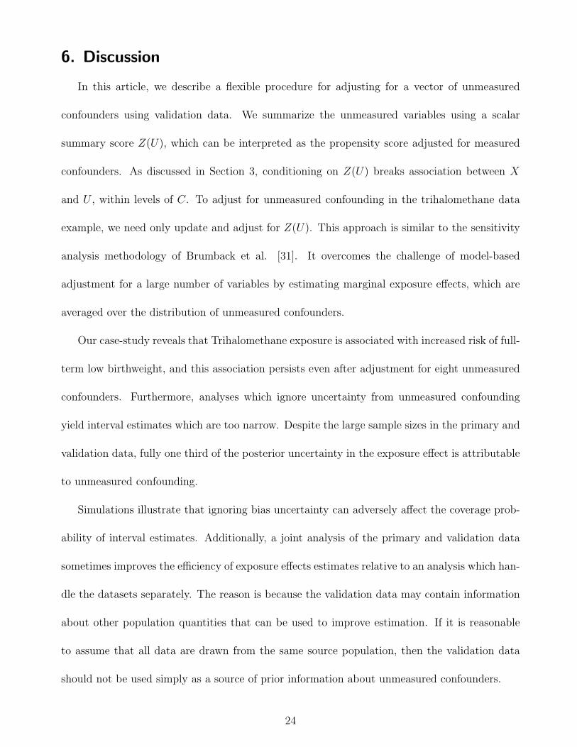
6. Discussion
In this article, we describe a flexible procedure for adjusting for a vector of unmeasured
confounders using validation data. We summarize the unmeasured variables using a scalar
summary score Z(U), which can be interpreted as the propensity score adjusted for measured
confounders. As discussed in Section 3, conditioning on Z(U) breaks association between X
and U , within levels of C. To adjust for unmeasured confounding in the trihalomethane data
example, we need only update and adjust for Z(U). This approach is similar to the sensitivity
analysis methodology of Brumback et al. [31]. It overcomes the challenge of model-based
adjustment for a large number of variables by estimating marginal exposure effects, which are
averaged over the distribution of unmeasured confounders.
Our case-study reveals that Trihalomethane exposure is associated with increased risk of full-
term low birthweight, and this association persists even after adjustment for eight unmeasured
confounders. Furthermore, analyses which ignore uncertainty from unmeasured confounding
yield interval estimates which are too narrow. Despite the large sample sizes in the primary and
validation data, fully one third of the posterior uncertainty in the exposure effect is attributable
to unmeasured confounding.
Simulations illustrate that ignoring bias uncertainty can adversely affect the coverage prob-
ability of interval estimates. Additionally, a joint analysis of the primary and validation data
sometimes improves the efficiency of exposure effects estimates relative to an analysis which han-
dle the datasets separately. The reason is because the validation data may contain information
about other population quantities that can be used to improve estimation. If it is reasonable
to assume that all data are drawn from the same source population, then the validation data
should not be used simply as a source of prior information about unmeasured confounders.
24

A limitation of our method is that it ignores variability in the empirical estimate of equation
(6). While this quantity is unbiased for P (Y,X|C) in equation (5), it may have high variance.
Supplying more validation data will alleviate this problem, but also at issue is the dimension of U
and the nature of the dependence of P (Y |X, C, U)P (X|C, U) on U . If the bias parameters ξ and
γ are large in magnitude, meaning that U contains powerful confounders, then the variability of
P (Y |X, C, U)P (X|C, U) will increase. To capture this variability, one extension of our method
would be to model uncertainty in the quantity in equation using a Bayesian bootstrap [9].
Appendix
Parallelling arguments by Rosenbaum and Rubin [18], we detail the theoretical behind using
the summary score Z(U) in equations (1) and (2) for control of unmeasured confounders. For the
trihalomethane data, let Y{1} and Y{0} denote potential outcomes for birth weight for an infant
[32]. The quantity Y{1} models the birth weight when the mother is exposed to trihalomethane
≥ 60µ/L, and takes value one if the infant has full term low birth weight and zero otherwise.
The quantity Y{0} models the corresponding potential outcome for birth weight assuming the
mother has trihalomethane less than 60µ/L. Let
Y = Y{X} =
Y{1} if X = 1
Y{0} if X = 0
denote the observed potential outcome. Following convention for causal inference in observa-
tional data, we assume that there is no interference between units and that conditional on (C, U),
there is no unmeasured confounding, meaning that (Y{1}, Y{0}) ⊥⊥ X|(C, U) [32]. This implies
that
P (Y |X, C, U) = P (Y{X}|X, C, U) = P (Y{X}|C, U)
25

for X = 0, 1. Effect measures computed from P (Y |X, C, U) have a causal interpretation.
Theorem 1: Assume that the model in equation (2) is correct, where Z(U) = γT U . Then
X ⊥⊥ U |C, Z(U).
Proof: Following Rosenbaum and Rubin [18] Theorem 1, it suffices to show that P (X =
1|U,C, Z(U)) = P (X = 1|C, Z(U)). We have E{P (X = 1|U,C, Z(U))|Z(U), C} = E{(1 +
exp(γT C + Z(U))−1|Z(U), C} = (1 + exp(γT C + Z(U))−1. When Z(U) is fixed, then the right
hand side does not depend on U , proving the identity.
In principle, this result could be generalized to exposure models other than that given in
equation (2). Any function of U , denoted Z(U), will satisfy equation (3) provided that P (X =
1|C, U) depends on U only through Z(U).
The following theorem shows that effect measures computed from the conditional distribu-
tion P (Y |X, C, Z(U)) have a causal interpretation. To control for confounding bias due to U ,
it suffices to stratify on (C, Z(U)). We can estimate the exposure effect by using models which
assume that Y ⊥⊥ U |X, C, Z(U).
Theorem 2: Assume that (Y{1}, Y{0}) ⊥⊥ X|(C, U) and that X ⊥⊥ U |C, Z(U), then (Y{1}, Y{0}) ⊥
⊥ X|(C, Z(U)).
Proof: Again, following Theorem 3 of Rosenbaum and Rubin [18], we show that
P (X = 1|Y0, Y1, C, Z(U)) = P (X = 1|C, Z(U)) = P (X = 1|C, U).
26

We have
P (X = 1|Y0, Y1, C, Z(U)) = E{P (X = 1|Y0, Y1, C, Z(U), U)|Y0, Y1, C, Z(U)}
= E{P (X = 1|Y0, Y1, C, U)|Y0, Y1, C, Z(U)} (10)
= E{P (X = 1|C, U)|Y0, Y1, C, Z(U)} (11)
= E{(1 + exp(γT C + Z(U))−1|Y0, Y1, C, Z(U)}
= (1 + exp(γT C + Z(U))−1
= P (X = 1|C, U).
Equation (10) holds because Z(U) is a function of U , while equation (11) holds because (Y{1}, Y{0}) ⊥
⊥ X|(C, U).
References
[1] S. Greenland. Multiple bias modelling for analysis of observational data (with discussion).
J R Stat Soc Ser A, 168:267–306, 2005.
[2] S. Schneeweiss. Sensitivity analysis and external adjustment for unmeasured confounders in
epidemiologic database studies of therapeutics. Pharmacoepidemiol Drug Saf, 15:291–303,
2006.
[3] P.R. Rosenbaum and D.B. Rubin. Assessing sensitivity to an unobserved binary covariate
in an observational study with binary outcome. J R Stat Soc Ser B, 45:212–8, 1983.
[4] T.J. VanderWeele. The sign of the bias of unmeasured confounding. Biometrics, 2007.
[5] T. Sturmer, S. Schneeweiss, J. Avorn, and R.J. Glynn. Adjusting Effect Estimates for
27
Unmeasured Confounding with Validation Data using Propensity Score Calibration. Am J
Epidemiol, 162:279–289, 2005.
[6] D.Y. Lin, B.M Psaty, and R.A. Kronmal. Assessing the sensitivity of regression results to
unmeasured confounders in observational studies. Biometrics, 54:948–63, 1998.
[7] L. C. McCandless, P. Gustafson, and A. R. Levy. A sensitivity analysis using information
about measured confounders yielded improved assessments of uncertainty from unmeasured
confounding. J Clin Epidemiol (in press).
[8] L.C. McCandless, P. Gustafson, and A.R. Levy. Bayesian sensitivity analysis for unmea-
sured confounding in observational studies. Stat Med, 26:2331–47, 2007.
[9] A. Gelman, J.B. Carlin, H.S. Stern, and D.B. Rubin. Bayesian Data Analysis, 2nd edition.
Chapman Hall/CRC, New York, 2004.
[10] W. Schill and K. Drescher. Logistic analysis of studies with two-stage sampling: A com-
parison of four approaches. Stat Med, 16:117–132, 1997.
[11] N.E. Breslow and R. Hulobkov. Weighted likelihood, pseudo-likelihood and maximum
likelihood methods for logistic regression analysis of two-stage data. Stat Med, 16:103–116,
1997.
[12] S. Wacholder and CR Weinberg. Flexible Maximum Likelihood Methods for Assessing Joint
Effects in Case-Control Studies with Complex Sampling. Biometrics, 50:350–357, 1994.
[13] L. Yin, R. Sundberg, X. Wang, and D.B. Rubin. Control of confounding through secondary
samples. Stat Med, 25:3814–25, 2006.
28

[14] S.J.P. Haneuse and J.C. Wakefield. Hierarchical Models for Combining Ecological and
CaseControl Data. Biometrics, 63:128–136, 2007.
[15] C. Jackson, N. B. Best, and S. Richardson. Hierarchical related regression for combining
aggregate and individual data in studies of socio-economic disease risk factors. J R Stat
Soc Ser A, 171:159–78, 2008.
[16] J. Molitor, C. Jackson, N. B. Best, and S. Richardson. Using Bayesian graphical models to
model biases in observational studies and to combine multiple data sources: Application to
low birth-weight and water disinfection by-products. (under review).
[17] N. Chatterjee, Y.H. Chen, and N.E. Breslow. A pseudoscore estimator for regression prob-
lems with two-phase sampling. J Am Stat Assoc, 98:158–169, 2003.
[18] P.R. Rosenbaum and D.B. Rubin. The central role of the propensity score in observational
studies for causal effects. Biometrika, 70:41–57, 1983.
[19] M.B. Toledano, M.J. Nieuwenhuijsen, N. Best, H. Whitaker, P. Hambly, C. de Hoogh,
J. Fawell, L. Jarup, and P. Elliott. Relation of Trihalomethane Concentrations in Public
Water Supplies to Stillbirth and Birth Weight in Three Water Regions in England. Environ
Health Perspect, 113:225–232, 2005.
[20] N.T. Molitor, C. Jackson, S. Richardson, and Best N. Bayesian graphical models for com-
bining mismatched data from multiple sources: Application to low birth-weight and water
disinfection by-products. Under review.
[21] L. C. McCandless, P. Gustafson, and P. C. Austin. Bayesian propensity score analysis for
observational data. (Under review).
29

[22] P.C. Austin and M.M. Mamdani. A comparison of propensity score methods: A case-study
estimating the effectiveness of post-AMI statin use. Stat Med, 25:2084–106, 2005.
[23] Z. Fewell, D. Smith, and J. A. C. Sterne. The Impact of Residual and Unmeasured Con-
founding in Epidemiologic Studies: A Simulation Study. Am J Epidemiol, 166:646, 2007.
[24] S. Greenland. The impact of prior distributions for uncontrolled confounding and response
bias: A case study of the relation of wire codes and magnetic fields to childhood leukaemia.
J Am Stat Assoc, 98:47–54, 2003.
[25] S. Schneeweiss, R.J. Glynn, E.H. Tsai, J. Avorn, and D.H. Solomon. Adjusting for unmea-
sured confounders in pharmacoepidemiologic claims data using external information: The
example of cox2 inhibitors and myocardial infarction. Epidemiol, 16:17–24, 2005.
[26] M.A. Hernan, S. Hernandez-Diaz, M.M. Werler, and Mitchell A.A. Causal knowledge as a
prerequisite for confounding evaluation: An application to birth defects epidemiology. Am
J Epidemiol, 155:176–84, 2002.
[27] P. Gustafson. On model expansion, model contraction, identifiability, and prior information:
two illustrative scenarios involving mismeasured variables. Stat Sci, (in press), 2005.
[28] A. Gelman. Parameterization and Bayesian Modeling. J Am Stat Assoc, 99:537–546, 2004.
[29] P. Gustafon. Sample size implications when biases are modelled rather than ignored. J R
Stat Soc Ser A, 169:883–902, 2006.
[30] V. Viallefont, A.E. Raftery, and S. Richardson. Variable selection and Bayesian model
averaging in case-control studies. Stat Med, 20:3215–3230, 2001.
30

[31] B.A. Brumback, M.A. Hernan, S. Haneuse, and J.M. Robins. Sensitivity analyses for
unmeasured confounding assuming a marginal structural model for repeated measures.
Statistics in Medicine, 23:749–767, 2004.
[32] J.K. Lunceford and M. Davidian. Stratification and weighting via the propensity score in
estimation of causal treatment effects: A comparative study. Stat Med, 23:2937–60, 2004.noindent
Table 1: Odds ratios (95% interval estimates) for the association between covariates and risk offull-term low birthweight.
Description Odds ratio (95% interval estimate)NAIVE BAYES FREQ
Trihalomethanes exp(β) 2.27 (1.68, 3.06) 2.03 (1.37, 2.93) 2.08 (1.54, 2.81)> 60µg/L
Mother’s age≤ 20 exp(ξ1) 0.35 (0.16, 0.77) 0.32 (0.15, 0.66) 0.34 (0.16, 0.76)20 - 24 exp(ξ2) 1.86 (1.29, 2.66) 1.76 (1.24, 2.47) 1.88 (1.30 , 2.68)25 - 29∗ . 1.0 1.0 1.030 - 34 exp(ξ3) 0.67 (0.42, 1.05) 0.61 (0.40, 0.95) 0.66 (0.42, 1.05)≥ 35 exp(ξ4) 0.89 (0.53, 1.47) 0.87 (0.53, 1.40) 0.89 (0.53, 1.47)
Male baby exp(ξ5) 0.87 (0.65, 1.16) 0.84 (0.64, 1.12) 0.86 (0.64, 1.15)∗ Reference group
31

Table 2: Odds ratios (95% interval estimates) for the association between covariates and risk offull-term low birthweight in the MCS data alone (m = 1333).
Description Odds ratio (95% interval estimate)Adjusting for Cj only Adjusting for Cj and Uj
Trihalomethane > 60µg/L 2.52 (1.03, 6.15) 2.39 (0.94, 6.11)
Mother’s age≤ 20 0.54 (0.08, 3.47) 0.27 (0.04, 1.88)20 - 24 1.81 (0.66, 4.97) 0.99 (0.33, 2.98)25 - 29∗ 1.0 1.030 - 34 0.37 (0.09, 1.48) 0.52 (0.12, 2.18)≥ 35 0.79 (0.19, 3.19) 1.31 (0.30, 5.73)
Male baby 0.92 (0.39, 2.13) 0.80 (0.33, 1.92)
Lone parent family . 1.20 (0.38, 3.80)Number of live children . 0.86 (0.69, 1.07)Smoking during pregancy . 4.08 (1.34, 12.40)Non-white etnicity . 3.88 (1.00, 15.11)Alcohol during pregancy . 1.77 (0.97, 3.22)Body mass index† (Kg/m2) . 0.75 (0.38, 1.49)Income (1=Low, 2=Med, 3=High) . 0.44 (0.17, 1.18)High school diploma . 1.07 (0.43, 2.68)∗ Reference group† Measured prior to pregnancy
32
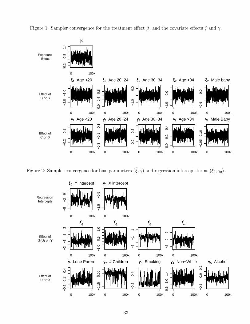
Figure 1: Sampler convergence for the treatment effect β, and the covariate effects ξ and γ.
Exposure Effect
0.2
0.8
1.4
ββ
0 100k
Effect of C on Y
−2.
0−
1.0
ξξ1 Age <20
0 100k
0.0
0.4
0.8
ξξ2 Age 20−24
0 100k
−1.
00.
0
ξξ2 Age 30−34
0 100k
−1.
00.
0
ξξ2 Age >34
0 100k
−0.
60.
0
ξξ2 Male baby
0 100k
Effect of C on X
−0.
20.
1
γγ1 Age <20
0 100k
−0.
3−
0.1
0.1
γγ2 Age 20−24
0 100k
0.0
0.2
γγ2 Age 30−34
0 100k
0.0
0.2
0.4
γγ2 Age >34
0 100k
−0.
050.
10
γγ2 Male Baby
0 100k
Figure 2: Sampler convergence for bias parameters (ξ, γ) and regression intercept terms (ξ0, γ0).
Regression Intercepts
−5
−2
0
ξξ0 Y intercept
0 100k
−1.
5−
0.5
γγ0 X intercept
0 100k
Effect of Z(U) on Y
−3
−1
13
ξξ~
1
0 100k
−1.
00.
52.
0
ξξ~
2
0 100k
−3
−1
1
ξξ~
3
0 100k
−2
02
ξξ~
4
0 100k
Effect of U on X
−0.
20.
10.
4
γγ~1 Lone Parent
0 100k
−0.
150.
00
γγ~2 # Children
0 100k
−0.
20.
4
γγ~3 Smoking
0 100k
0.6
1.0
1.4
γγ~4 Non−White
0 100k
−0.
30.
00.
2
γγ~5 Alcohol
0 100k
33

Figure 3: Sampler convergence the deviance evaluated over MCMC iterations of (β, ξ, ξ, γ, γ).
1423
014
260
Deviance
0 50k 100k
34

Fig
ure
4:Per
form
ance
ofpoi
nt
and
inte
rval
esti
mat
esfo
rth
eex
pos
ure
effec
tβ
calc
ula
ted
usi
ng
eith
erB
AY
ES,FR
EQ
orN
AIV
E.T
he
top
pan
els
des
crib
eth
ebia
s(s
imula
tion
stan
dar
der
ror
(SE
)<
0.02
)an
dva
rian
ce(S
E<
0.00
6)of
poi
nt
esti
mat
es.
The
bot
tom
pan
els
des
crib
eth
eco
vera
gepro
bab
ility
(SE
<4%
)an
dle
ngt
h(S
E<
0.00
7)of
80%
inte
rval
esti
mat
es.
BA
YE
S
025
050
010
00
−0.0500.050.10.15
00.0250.05
Bias
FR
EQ
025
050
010
00
−0.0500.050.10.15
00.0250.05
NA
IVE
025
050
010
00
−0.0500.050.10.15
00.0250.05
Variance
m −
Sam
ple
Siz
e of
Val
idat
ion
Dat
a
025
050
010
00
50%60%70%80%90%
0.50.60.70.80.9
Coverage Probability
m −
Sam
ple
Siz
e of
Val
idat
ion
Dat
a
025
050
010
00
50%60%70%80%90%
0.50.60.70.80.9
m −
Sam
ple
Siz
e of
Val
idat
ion
Dat
a
025
050
010
0050%60%70%80%90%
0.50.60.70.80.9
Average Interval Length
35


