
Quality Choice: Effects of Trade, Transportation Cost, and Relative
Country Size.1
Volodymyr Lugovskyy
(Georgia Institute of Technology)
Alexandre Skiba
(University of Wyoming)
November 2009
We introduce a generalized iceberg transportation cost, which combines per-unit and ad-valorem
components, into a monopolistic competition model of trade with endogenous quality choice. In
equilibrium, quality of exports increases in per-unit component of the iceberg due to an Alchian-
Allen effect. Because of this firms in smaller countries that export larger share of their output
choose higher quality. Next we show empirically on the sample of US imports that larger
countries tend to export lower priced goods especially in those industries where transportation
cost has a larger per-unit component.
JEL F1, R1
1 We thank David Hummels, Johannes Moenius, Richard Pomfret, the seminar audiences at Purdue U,U of
Wyoming, GA Tech, Kyiv School of Economics, and the participants of the 2009 EITI Conference in Tokyo, and
2009 EITG Conference in Melbourne.

1
1. Introduction
Krugman (1979) describes how specialization can occur within an increasing returns to
scale industry or even within a differentiated product. An important implication of his seminal
work lies in a formal description of the home market effect. It states that specialization due to
increasing returns can be detected by the relationship between the quantity of exports and the
market size. More than proportional correlation indicates that larger countries specialize in the
increasing returns sector.
Further pursuing this line of research, Schott (2004) and Hallak (2003) detect substantial
within-product specialization and point out that rich countries specialize in the higher quality
products. In particular, Schott’s results highlight considerable vertical international
specialization even within the most narrowly defined product categories.
This paper contributes to existing literature by showing theoretically and confirming
empirically that smaller countries have comparative advantage in producing higher priced and
higher quality goods. The key factor of our result is the non-ad-valorem nature of transportation
cost. If at least a part of transportation cost does not depend on the value of the good, the relative
price of the higher price goods is lower for importing destinations. As first pointed out by
Alchian and Allen, it creates an incentive to “ship the good apples out.” We combine these ideas
in a model where generalized transportation costs and quality are jointly determined. In such
setup, the smaller the domestic market relative to the rest of the world, the higher are the
incentives for an individual producer to “grow better apples” because higher share of its output is
subject to the Alchian-Allen effect.
Variation in unit value is not accounted for by traditional model of trade with product
differentiation and increasing returns to scale. In those models specialization manifests itself as

2
the home-market effect. Hanson and Xiang (2004) show theoretically and confirm empirically
that the strength of the home market effect prominently depends on the ad valorem size of
transportation cost. The ad valorem incidence of transportation is however different for goods of
different unit values. Hummels and Skiba (2004) show that transportation costs are less than
one-to-one proportional to the unit value of shipped goods and therefore lead to changes in
relative demands because higher priced goods have lower ad valorem equivalent of
transportation costs (the Alchian-Allen effect). As a result, countries tend to export higher priced
goods to more remote destinations. In this paper we integrate insights from the previous
literature to investigate whether the nature of the transportation costs affects specialization in the
models of trade in differentiated goods produced under increasing returns to scale.
We introduce a generalized iceberg transportation cost into a monopolistic competition
model of trade with endogenous quality choice. In doing so, we retain analytical simplicity of
the traditional iceberg assumption but allow for both a per-unit and an ad valorem component of
transportation costs. The resulting model predicts a systematic negative relation between
country size and export prices. In equilibrium, quality increases in per-unit component of the
iceberg and in firm’s export share. This is because the firms that export more of their output face
a stronger incentive to upgrade quality as larger share of their output incurs transportation cost.
In the corner equilibrium with one-way trade in the differentiated sector, both the export share
and quality decrease in the exporter country size.
Intuitively, country size matters relatively less when transportation costs are lower. So, if
higher priced goods face lower ad valorem transportation cost, the location of the higher
transportation cost industry is more sensitive to the transportation cost. Our theory can be
anecdotally intuited by notorious examples of small countries specializing in high quality goods
3
such as Swiss watches, Belgian chocolate, or Vietnamese Kopi Luwak coffee. Japanese photo
lenses.
In the empirical exercise we first estimate industry level transportation cost functions to
determine the degree to which transportation costs co-vary with the product unit value. Next
using a sample of US imports we show empirically that larger countries tend to export lower
priced goods. The negative effect of market size on the price of exports is stronger in those
industries where transportation costs have a larger per-unit component. This finding raises a
possibility that increasing returns play a larger role in explaining international trade than
previously thought. This is because the customary approach that uses value of trade to identify
the home market effects might underestimate the effect of country size on exports because price
and quantity are effected in opposite directions. This supposition is borne out by the data.
According to our estimates home market effect is present in about a quarter to a third more
industries when volume of exports is measured by quantity rather than value.
2. Theoretical Framework
We augment Samuelson iceberg transportation cost to investigate the relation between
country size and quality choice in the presence of Alchian-Allen effect. In particular, we extend
the well-known home-market effect model of Helpman and Krugman (1985) to the case of
endogenous quality choice and augmented transportation cost. The major novelty is that the
augmented transportation cost includes a per-unit component, which creates an incentive for
exporters to upgrade quality due to Alchian-Allen effect. The incentive is stronger in a smaller
country, given that in a smaller country firms devote larger share of the output to exports. As a

4
result, the smaller country will produce and export higher price and higher quality differentiated
goods.
2.1. Preferences and Production
The world consists of two countries, Home and Foreign, with population L and L*, ,
respectively. We set up the model from Home’s perspective. Preferences of a representative
consumer are defined over a numeraire good 0q and many differentiated goods:
(1) ( )( ) ( )/ 11 /1
0 k kkU q q
µσ σσ σµ λ
−−− =
∑ 1σ > ,
where kq is consumption of the kth
good, and kλ is a corresponding quality multiplier.
Labor is the only factor of production and is supplied inelastically. Each consumer is
endowed with one unit of labor. The numeraire sector is characterized by perfect competition and
constant returns to scale. One unit of labor can produce w units of the numeraire in Foreign and 1
unit in Home. The numeraire is traded at zero cost. We assume that the numeraire sector is large
enough for both countries to have strictly positive output of the numeraire. The introduction of the
numeraire in the model simplifies the balance of trade calculation and ties the wage to productivity
in the numeraire sector.
Differentiated varieties are produced by monopolistically competitive firms. The cost
function is characterized by a fixed labor requirement α , and a marginal labor requirement kc ,
which is a function of a chosen quality kλ and productivity parameters A>0 and Z>02:
(2) ( ) ( )1/ exp /k k
c A Zλ= .
2 This type of unit labor function was first introduced by Flamm and Helpman (1987). A similar function in
conjunction with CES preferences is used by Hummels and Klenow (2005).

5
2.2. Augmented Transportation Cost
It is difficult to derive a structural functional form of the transportation cost. For
example, if we focus on the vessel mode of transportation, international shipping is a
sophisticated technology which includes both fixed and variable cost components. The fixed
cost component is a function of port infrastructure, where the variable cost depends on distance,
volume of trade, and good-specific characteristics (Hummels, Lugovskyy and Skiba; 2009).
Our goal is to suggest a functional form which would capture both ad-valorem and per-
unit components of transportation cost, and, at the same time, would preserve the analytical
simplicity and tractability. For this purpose, we assume a part of transportation cost to be
incurred in terms of the final good (ad-valorem component) and part in terms of units of labor
(per-unit component). In particular, to transport one unit of the differentiated good k it takes
( )1ϕ − units of the good and u units of labor.
The shippers are paid by producers with the final good at the market factory gate price.
Due to labor mobility assumption, the labor employed in shipping industry is rewarded at the
market wage w, which corresponds to ( ) ( )1 /k
cσ σ− units of the final good k at the market
price. Shipping industry is characterized by perfect competition, zero profits, and pricing its
services at marginal cost of shipping.
The total shipping charge, f, expressed in terms of the numeraire is
(3) ( )1k k
f p uwϕ= − + .
The elasticity of the augmented shipping charge with respect to price varies between 0 and 1:
(4)
1
ln 1 11
ln 1
k
k k
d f u
d p c
σ
σ ϕ
− −
= + −
.

6
As 0u → , the transportation cost converges to Samuelson iceberg and the elasticity approaches
to 1. Alternatively, as 1ϕ → , the elasticity approaches 0, since the transportation cost converges
to the per-unit cost. If we abstract from extremes, the elasticity is between 0 and 1, which
signifies that both per-unit and ad-valorem components play an important role in the total
transportation charge. These considerations are important for estimating the functional form of
the total transportation cost in the empirical section.
In the model, on the other hand, we would like to preserve the tractability of the
transportation function. For this purpose, we express transportation cost in ad-valorem terms.
Under the above assumptions, the augmented iceberg cost function of delivering a differentiated
good k from Home to Foreign is:
(5) 1
1 kk
k k
f u
p c
στ ϕ
σ
−= + = + .
Note that, contrary to the traditional Samuelson iceberg, the augmented iceberg is a
function of the marginal cost of production. In particular, it is decreasing in the marginal cost,
meaning that higher price goods have lower ad-valorem cost of transportation. Given the
positive correlation between price and quality, the augmented iceberg implies that a higher
quality good faces a lower ad-valorem transportation cost.
2.3. Quality in Autarky Equilibrium
In autarky, the profit-maximizing quality level is equal to the productivity parameter Z:
(6) autarkyZλ = .
3
3 This a partial case of equilibrium with trade in which the export share is equal to zero. The corresponding
derivations are given in the next subsection.

7
2.4 Quality in Trade Equilibrium
Consider the profit function of a firm producing kQ units of differentiated good k in
Home:
(7) ( )1k k k k fk k hsk k k kp Q ES p Q ES c Qπ τ α= − + − − ,
where kp and fk
p are the prices charged by firm k in Home and in Foreign, respectively;
kES is the share of exported quantity in the firm’s output;
kτ is the generalized iceberg transportation cost [defined by (5)];
α and kc are the fixed and marginal unit labor requirements, respectively;
w is the wage in Home.
By solving the profit maximizing problem with respect to kQ and kλ , we can find the optimal
quality level:
(8) 1 kk k
k
u cZ ESλ
τ
= −
,
where ( )k ku c τ is positively correlated with the share of the per-unit component in the total
iceberg cost. Note that if the share of exports is equal to zero, as in autarky, the result coincides
with (6). If kES is non-decreasing in kλ , the optimal quality choice, kλ , is unique, since both
sides of the above equation increase with kλ .4
The next two observations are expressed as lemmas.
Lemma 1: If and only if transportation cost contains a per unit part, exporters produce higher
price and higher quality goods than non-exporters.5
4 The Export Share will be shown to be non-decreasing in quality in the next subsection.
5 Though stemming from different set-up, exporters produce higher price and higher quality goods also in Baldwin
and Harrigan (2008) model.

8
Proof: Follows directly from (8).■
Intuitively, a negative correlation between the marginal cost of production and ad-
valorem transportation costs provides an additional incentive for exporters to produce higher
quality goods. This correlation is negative only in the presence of the per-unit part of
transportation cost, and it does not affect non-exporters.
Lemma 2: The equilibrium price and quality of exported goods increase with the per unit part
of transportation cost and with the share of exports.
Proof: Follows directly from (8).■
From (8), the magnitude of the (negative) effect of quality on the generalized iceberg
increases with per-unit component u. Consequently, the larger the share of per-unit part in the
total transportation cost, the stronger is the incentive to produce higher quality good. Moreover,
since export share increases the weight of transportation cost in overall profit calculation [see
equation (7)], it also increases the incentive to invest in higher quality.
2.5. Firm-Level Export Share
While quality increases with the firm-level export share, the export share in itself is
endogenous. In particular, the functional form of the export share depends on whether in
equilibrium we observe a two-way or one-way trade.
2.5.1. Firm Level Export Share in the Two-Way Trade Equilibrium
As in Helpman and Krugman (1985) model the export share of an individual firm is
independent of the country sizes in the interior, two-way trade, equilibrium. 6
.
6 Equation 10.18 (page 207) deomstrates this result for Helpman-Krugman (1985) model, and it can easily be
extended to our setting.

9
2.5.2. Firm Level Export Share in the One-Way Trade Equilibrium
Assume that the parameters of the model are such that Home is the sole producer and
exporter of differentiated goods. Given the Cobb-Douglas upper case utility function, consumers
in each country spend a constant share of income, µ , on differentiated goods:
( )1k k kL NQ ES pµ = − ( )* k k k fkwL N Q ES pµ τ= .
where µ is the income share spent on differentiated varieties; L and L* are the labor
endowments in Home and Foreign, respectively; N is the number of Home’s differentiated
varieties; kQ is an output per variety k (all varieties are symmetric); w is wage in Foreign; kES
is an export share; kp and fkp are prices charged in Home and Foreign, respectively; and kτ is
an augmented iceberg transportation cost.
By plugging in the equilibrium values, ( )1 /kQ α σ α= − , ( )1k kp c σ σ= − , and
( )1fk k kp c στ σ= − , we get:
( )1 kL N ESµ ασ= − ( )* kL w N ESµ ασ= ,
from which we derive the equilibrium export share:
(9) 1 1* *
k
L YES
L wL Y Y= − = −
+ +.
Thus in the corner equilibrium, the export share is decreasing in the relative size of the
exporter. By plugging this result into (8) we get
(10) ( )exp
1 1 1*
k
k k
A ZY Z
Y Y u
ϕ λ
λ
− = + −
+ ,
which allows us to formulate and prove Lemma 3.

10
Lemma 3: In the corner on-way trade equilibrium, the quality level is decreasing in the GDP of
the exporter. This effect is increasing in the per-unit and decreasing in the ad-valorem share of
the transportation cost.
Proof: Follows directly from (10).■
2.6 . Home Market Effect Revisited
Starting with Krugman (1980) and Helpman and Krugman (1985) the literature on home
market effect focuses on the case of interior equilibrium in which, ceteris paribus, larger country
exports proportionally more varieties than smaller country. We consider a different angle of this
issue. Let us combine all differentiated sectors in one industry and assume a perfectly
asymmetric distribution of productivities between Home and Foreign. (as, e.g., in Fisher,
Dornbush, and Samuelson 1977). The conditions defining the industries in which industries we
should observe corner equilibrium are similar to the conditions derived by Helpman and
Krugman (1985).
It is possible to show that a larger country will have more sectors in which it is a sole
exporter than a smaller country. Thus, at industry level, the home market effect can stem not
only form the fact that larger country produces more varieties in sectors with interior
equilibrium, but also from the fact that larger country is a sole exporter in more sectors than a
small country is.7
If the Home Market Effect stems even partially form the second channel, the magnitude
of the Home Market Effect should be greater when we compare the quantities exported than
when we compare the values exported, since smaller country will produce higher quality goods
and charge higher prices for its exports.
7 The proof of this statement is available upon request form the authors.

11
3. Empirics
3.1. Data
Our data cover the US imports from all exporters worldwide, measured at 10 digit level
of the Harmonized Classification System (16800+ categories) in 2000.8 Denote a 10-digit
commodity category by k. For commodity k imported form country i the data include the f.o.b.
value, ikV , quantity, ikQ , and shipping charge, ikS . We compute the unit value of commodity k
from country i as /ik ik ikp V Q= , and the corresponding freight rate as /ik ik ikf S Q= . We refer to
HS 10 category as “product”, or “good”. For GDP and GDP per capita data we used the World
Development Indicators data.9
3.2. Estimating Industry Transportation Cost Functions
Theory indicates that relative delivered price and hence the quality of exports crucially
depend on the specific part of transportation cost. In order to test whether transportation cost is
iceberg and to determine the degree to which transportation cost deviates from iceberg, we
estimate a transportation cost function that allows for flexible relation between price and
transportation cost. For every industry K the following transportation cost function is estimated
using a subsample of US imports in from 2002 to 2004:10
.
(11) 50% 90%
0 1 2 3 4ln ln lnist K K ist K i K ist K ist Kt t istt
f p Dist Air Air Dα α α α α β ε= + + + + + +∑
where isf is per unit freight charge to deliver a unit of shipment s from country i ; isp – f.o.b.
unit value of good in shipment s imported from country i ; K – either HS 2 or HS 6 digit
8 For trade data, we used the US Census Imports of Merchandise.
9 Data source: World Bank.
10 The choice of years 2002-2004 is motivated by the ability to confirm that our estimation results are robust to
using the US imports restricted to single shipments.

12
industry index; iDist – distance to i ; iY – GDP of country i ; %X
isA – dummy variable, which is
equal to 1 if for HS 10 digit product s in country i more than X% of value of exports is
transported by air; tD is a year fixed effect.
This form of transportation cost function is similar to the commonly used in trade
literature (see, for example, Hummels 1999,and Hummels and Skiba 2004). There are two
differences. First, we recognize that transportation technology might differ for air and vessel.
Intermodal substitution is potentially an important issue in the estimation of industry
transportation cost functions. Many HS 10-digit categories contain goods imported by air and by
vessels. If we combine all shipments into one pooled regression our price elasticity will be
affected by the intermodal substitution. The goods that are shipped by air tend to be of higher
unit values. This is potentially an issue if quality does not affect the mode of transportation. In
order to partially correct for this possibility we estimate equation (11) with dummies for air
shipments. Second, in the above specification, the freight rate is a function of the price, while
according to our theory the price is a function of the freight rate. To handle simultaneity, we
instrument for prices using the exogenous variables, such as the (weighted) average price of a
given HS10 digit commodities exported by the rest of the world for a given year, tariff dummy11
,
and per capita GDP of exporter.
Our primary interest lies in the price elasticity of transportation cost, 1Kα . Consistent
with the intuition of our theretical result in equation (4), if 1 0Kα = , transportation cost is per-
unit and does not depend on price; if 1 1Kα = , transportation cost isad-valorem; and, finally, if
10 1Kα< < , transportation cost contains both per-unit and ad-valorem components.
11
Half of the observations are subject to zero or miniscule tariff. Thus instead of using the log of tariff rate as in
Hummels and Skiba (2004), we use the tariff dummy equal to 1 if tariff is less than 1% and 0 otherwise.
13
Summary of the estimation results can be seen in Figures 1a (HS 2 digit) and 1b (HS 6
digit). Based on available data we could estimate transportation parameters for 97 HS 2 and
4644 HS 6 industries, 85 and 3848 of them were significant at 5% level, 81 and 3009 of those are
significantly different from the traditional iceberg based on a two-sided t-test of the hypothesis
that 1ˆ 1Kα = . There is also a substantial degree of variation across industries in the degree of
deviation from the standard iceberg.
3.3. Effect of Size on the Price of Exports
Next we investigate the relation between exporter’s size and the price of exports. Since
transportation is not iceberg for all industries, we expect size to lower the price of exports. This
correlation alone would be consistent with our theory but might also arise through some other
channel. A more persuasive case in favor of our explanation could be made if the negative effect
of market size on the price of exports were stronger for industries where transportation cost is
less like iceberg. In order to formally test the varying strength of the size-price connection we
use the following empirical specification:
(12) ( )0 1 2 3 4 5ln ln ln lnK
i i K i K i i iKP Y T Y T C Dβ β β β β β ε= + + + + + +
where K
iP – measure of exporter i ’s price in industry K (average price or Fisher’s ideal price
index); iY – measure of exporter i ’s market size (nominal GDP or market potential); iC –
vector of i specific cost shifters (GDP per capita, human capital, physical capital, labor); iD –
distance to i ; KT – vector of variables that reflect distortions to relative prices introduced by
transportation of goods from industry K

14
The price of country’s exports can be simply measured as a trade weighted average. Such
approach would however blend differences in price levels with differences in composition of
exports. Therefore, a price index could offer distinct advantages. We modify Hummels and
Klenow’s (2002) use of Fisher price index to construct a separate index for exporter i in industry
K .
1 12 2
ijK ijK
ijK ijK
ijk ijk ijk Wjk
k X k XK
i
Wjk ijk Wjk Wjk
k X k X
p q p q
Pp q p q
∈ ∈
∈ ∈
=
∑ ∑
∑ ∑
where j – US; ijKX – set of categories k imported from i to the US; Wjk
p – average price of
US imports in category k ; Wjkq – total quantity of US imports in category k .
We use nominal GDP and market potential as two alternative measures of the market
size. Market potential augments country’s GDP to include distance weighted GDP of its trading
partners. Following the Fujita, Krugman, and Venables (1999), and Hanson and Xiang (2004),
we calculate the market potential as:
j i
i i
j i ij
GDP AMP GDP
Dφ π≠
= +∑
where GDP – nominal GDP
ijD – distance from between i and j
iA – land surface area of country i
We set φ equal 0.92 using Hummels’s estimate of the distance coefficient in the gravity
model.12
12
Setting φ equal 0.92 is also consistent with Hanson and Xiang (2004)

15
The results of estimation are presented in tables 1a, 1b, 2a, and 2b. Table 1a and 1b report
estimated coefficients for pooled regression with prices defined at HS 2 and HS 6 levels,
respectively. Tables 2a and 2b report estimation results for similar specifications with industry
fixed effects. Industry fixed effects control for unobservable industry specific characteristics but
also remove some of the useful variation in the transportation cost parameters. The effect of size
on price is universally negative when statistically significant. The effect of size on the Fisher’s
ideal price index is consistently weaker than on the average price indicating that the change in
composition of exports plays a role in the lowering of the exports price with exporter’s size. Not
only larger exporters tend to export lower priced products they also tend to export more of the
lower priced exports. Consistently with the theoretical predictions industries whose
transportation costs are closer to iceberg (farther from 0 and closer to 1) exhibit a weaker
negative relation between market size and price of exports. This is evidenced by the positive
coefficient on the ( 1ˆ
Kα × size) interaction term.
3.4. Distinguishing Price from Quality
Product quality is not the only reason for variation in prices. We use approach suggested
by Hummels and Klenow (2003) to separate effect of market size on exporter’s quality. For
every HS 2-digit category we estimate the effect of market size on both price and quantity index .
(13)
( )
( )0 1 2 4 5
0 1 2 4 5
ln ln ln ln
ln ln ln ln
K K K K K K
i i K i i i iK
K K K K K K
i i K i i i iK
P Y T Y C D
Q Y T Y C D
β β β β β ε
γ γ γ γ γ ε
= + + + + +
= + + + + +
Vector of cost controls iC includes GDP per capita, human capital, physical capital, and labor
Quantity is measured as the quantity index in a similar fashion to the Fisher ideal price index
according to the following formula
16
1 12 2
ijK ijK
ijK ijK
ijk ijk Wjk ijk
k X k XK
i
ijk Wjk Wjk Wjk
k X k X
p q p q
Qp q p q
∈ ∈
∈ ∈
=
∑ ∑
∑ ∑
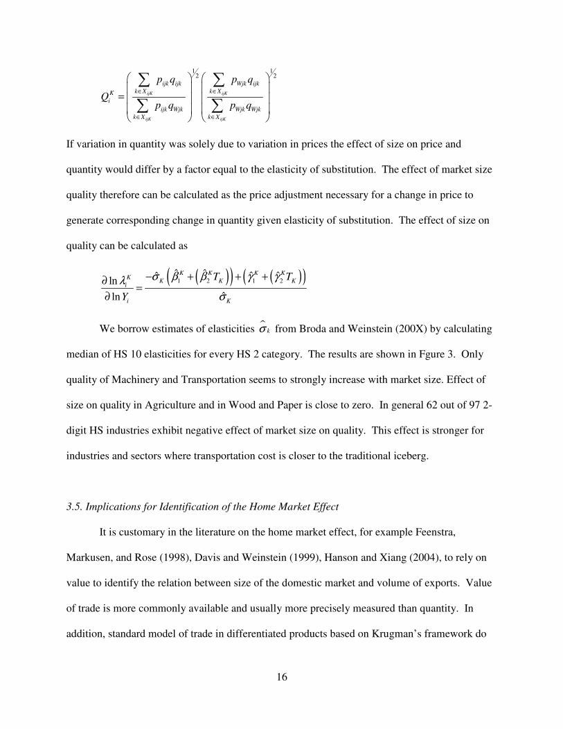
If variation in quantity was solely due to variation in prices the effect of size on price and
quantity would differ by a factor equal to the elasticity of substitution. The effect of market size
quality therefore can be calculated as the price adjustment necessary for a change in price to
generate corresponding change in quantity given elasticity of substitution. The effect of size on
quality can be calculated as
( )( ) ( )( )1 2 1 2ˆ ˆ ˆ ˆˆln
ˆln
K K K KK
K K Ki
i K
T T
Y
σ β β γ γλ
σ
− + + +∂=
∂
We borrow estimates of elasticities � kσ from Broda and Weinstein (200X) by calculating
median of HS 10 elasticities for every HS 2 category. The results are shown in Fgure 3. Only
quality of Machinery and Transportation seems to strongly increase with market size. Effect of
size on quality in Agriculture and in Wood and Paper is close to zero. In general 62 out of 97 2-
digit HS industries exhibit negative effect of market size on quality. This effect is stronger for
industries and sectors where transportation cost is closer to the traditional iceberg.
3.5. Implications for Identification of the Home Market Effect
It is customary in the literature on the home market effect, for example Feenstra,
Markusen, and Rose (1998), Davis and Weinstein (1999), Hanson and Xiang (2004), to rely on
value to identify the relation between size of the domestic market and volume of exports. Value
of trade is more commonly available and usually more precisely measured than quantity. In
addition, standard model of trade in differentiated products based on Krugman’s framework do
17
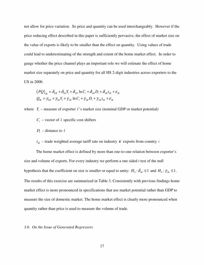
not allow for price variation. So price and quantity can be used interchangeably. However if the
price reducing effect described in this paper is sufficiently pervasive, the effect of market size on
the value of exports is likely to be smaller than the effect on quantity. Using values of trade
could lead to underestimating of the strength and extent of the home market effect. In order to
gauge whether the price channel plays an important role we will estimate the effect of home
market size separately on price and quantity for all HS 2-digit industries across exporters to the
US in 2000.
( ) 0 1 2 3 4
0 1 2 3 4
ln
ln
K K i K i K i K iK iKiK
iK K K i K i K i K iK iK
PQ Y C D t
Q Y C D t
δ δ δ δ δ ε
γ γ γ γ γ ε
= + + + + +
= + + + + +
where iY – measure of exporter i ’s market size (nominal GDP or market potential)
iC – vector of i specific cost shifters
iD – distance to i
iKt – trade weighted average tariff rate on industry K exports from country i
The home market effect is defined by more than one-to-one relation between exporter’s
size and volume of exports. For every industry we perform a one sided t test of the null
hypothesis that the coefficient on size is smaller or equal to unity: 0 1: 1KH δ ≤ and 0 1: 1KH γ ≤ .
The results of this exercise are summarized in Table 3. Consistently with previous findings home
market effect is more pronounced in specifications that use market potential rather than GDP to
measure the size of domestic market. The home market effect is clearly more pronounced when
quantity rather than price is used to measure the volume of trade.
3.6. On the Issue of Generated Regressors

18
Statistical significance of transportation cost function parameters in estimating equations
(12) is central for our conclusions about the effect of size on export’s price. Simple t-statistics
could be misleading because the parameters of the cost function are generated regressors
estimated from specification in equation(11). Unfortunately, there is no straightforward
adjustment for the generated nature of the parameters of the cost function. For example we
cannot construct the variance-covariance matrix of the estimated coefficients similarly to two
stage least squares estimator because our generated regressor is constructed from two estimates
obtained from two subsets of a dataset that is different from the dataset used in the second stage
regression.
Since the exact adjustment is not known we design a two stage bootstrap procedure to
estimate standard errors of the estimated coefficients. The bootstrap procedure performs 100
draws with replacement each time estimating equation (12) by HS 2-digit sampling strata. Every
time a sample is drawn we re-estimate transportation cost function (11) for air and vessel imports
on a randomly drawn sample of single shipments using HS 2-digit as sampling strata. The results
of the estimation are presented in Table 4.
We believe that the problem of generated regressors is not as severe in our application as
in others. First, all transportation cost function coefficients are estimated very precisely with
small standard errors. The value of the smallest t-statistics exceeds 2.3 for both air and vessel
transportation cost functions. The median of the t-statistics for both modes exceeds 21. Second,
there is significantly more variation in the estimated elasticities than in the sample variation of
the estimated elasticities is about an order of magnitude larger than the average.
4. Conclusions and Discussion

19
We find that when a good is exported by many countries the average price of exports is
lower for larger countries, although not universally. We show how this link between the size and
average price can arise from the interaction between the Alchian-Allen effect and the home
market effect. The effect of size on price is stronger when transportation cost co-varies less with
the unit value of the shipped good.
The empirical results are consistent with our theoretical predictions. Not only larger
countries tend to ship lower priced goods but also this negative relation is stronger when
transportation cost is less ad valorem. There can be potentially other reasons of why large
countries have lower export prices. In particular, large countries might choose a “high fixed cost
- low variable cost” technology due to larger size of the domestic market. Alternatively,
importers might consider a country of origin as additional factor of differentiation which might
force producers form large countries to charge lower export markups due to higher competition
with similar varieties. Unfortunately with the data in hands, we are not able to test what is
exactly the mechanism which lowers the export prices for large countries. In terms of theoretical
contribution, our message is that even if we assume endogenous technological choice and
differences in markups, larger countries have incentives to specialize in lower quality.
In this paper we do not model a relation between elasticity of substitution and quality.
The elasticities of substitution for high and low qualities are identical. This assumption of
convenience is not always innocuous because it is the interaction between the iceberg
transportation cost and elasticity that determine existence and relative strength of the home
market effect for high and low quality varieties.

20
References
Broda, Christian and Weinstein, David E. (2006), “Globalization and the Gains from Variety”,
Quarterly Journal of Economics, 121(2), 541-585
Choi, Yo Chul (2006) “Essays on Product Quality Differentiation and International Trade”,
Purdue University, Ph.D. Dissertation.
Robert C. Feenstra & James A. Markusen & Andrew K. Rose, 1998. "Understanding the Home
Market Effect and the Gravity Equation: The Role of Differentiating Goods," NBER Working
Papers 6804, National Bureau of Economic Research
Fujita, Masahisa; Krugman, Paul and Venables, Anthony J. The spatial economy: Cities, regions,
and international trade. Cambridge, MA: MIT Press, 1999.
Hanson and Xiang (2004): “The Home-Market Effect and Bilateral Trade Patterns,” The
American Economic Review, Vol. 94, No. 4. (Sep., 2004), pp. 1108-1129.
Hummels, David (2001) “Toward a Geography of Trade Costs”, Purdue University, mimeo
Hummels, David, Peter J. Klenow, 2002. "The Variety and Quality of a Nation's Trade," NBER
Working Papers 8712, National Bureau of Economic Research,
Hummels, David and Skiba, Alexandre (2004): "Shipping the Good Apples Out? An Empirical
Confirmation of the Alchian-Allen Conjecture," Journal of Political Economy, University of
Chicago Press, vol. 112(6), pages 1384-1402, December.
Krugman, Paul, and Elhanan Helpman (1985). Market Structure and Foreign Trade. The MIT
Press.
Hummels, David, Lugovskyy, Volodymyr, and Skiba, Alexandre (2009): “The Trade Reducing
Effects of Market Power in International Shipping”, Journal of Development Economics, vol.
89(1), pages 84-97
Schott, Peter (2004): “Across-Product versus Within-Product Specialization in International
Trade.” Quarterly Journal of Economics 119(2):647-678 (May 2004).
Samuelson, P. A. (1954), “Transfer Problem and the Transport Cost, II: Analysis of Effects of
Trade Impediments,” Economic Journal, 64, 264-289.

21
Table 1a. Effect of market size on export price at HS 2 digit level, pooled specifications.
Dep. variable Average price Fisher's ideal price index Average price Fisher's ideal price index
Measure of
size GDP GDP Market potential Market potential
(1) (2) (3) (4) (5) (6) (7) (8) (9) (10) (11) (12)
Size -0.134 -0.2 -0.175 -0.302 -0.324 -0.293 -0.076 -0.099 -0.081 -0.176 -0.194 -0.172
[13.98]** [4.74]** [3.01]** [11.76]** [7.57]** [3.69]** [8.47]** [2.91]** [0.38] [5.38]** [5.15]** [1.50]
Transportation cost parameters
0ˆ
Kα × size 0.084 0.051 0.026 0.016 0.045 0.036 0.019 0.012 [6.85]** [3.47]** [2.46]* [1.27] [4.32]** [3.28]** [2.21]* [1.33]
1ˆ
Kα × size 0.302 0.122 0.555 0.326 0.181 -0.007 0.382 0.233 [2.69]** [0.82] [5.84]** [2.62]** [1.79] [0.06] [4.52]** [2.37]*
0ˆ
Kα -2.275 -1.393 -0.84 -0.569 -1.511 -1.202 -0.789 -0.55
[7.26]** [3.62]** [3.16]** [1.77] [4.59]** [3.45]** [2.86]** [1.88]
1ˆ
Kα -14.509 -9.954 -17.05 -11.433 -12.663 -6.732 -15.033 -10.38 [5.28]** [2.66]** [7.33]** [3.64]** [4.12]** [1.86] [5.85]** [3.42]**
Distance 0.225 0.211 0.225 0.126 0.117 0.101 0.157 0.155 0.263 0.065 0.065 0.128
[5.58]** [5.53]** [5.10]** [3.79]** [3.64]** [2.72]** [3.75]** [3.91]** [5.80]** [1.91] [1.97]* [3.37]**
Cost controls
GDP p.c. 0.145 0.144 0.757 0.109 0.107 0.567 0.072 0.09 0.408 0.058 0.068 0.274 [8.48]** [8.87]** [6.01]** [7.74]** [7.80]** [5.37]** [4.40]** [5.80]** [6.80]** [4.32]** [5.19]** [5.44]**
Human cap. -0.186 -0.205 -0.203 -0.223 [3.30]** [4.33]** [3.41]** [4.46]**
Capital -0.246 -0.109 -0.326 -0.157 [3.31]** [1.74] [4.45]** [2.55]*
Labor 0.592 0.415 0.222 0.09 [4.22]** [3.53]** [2.49]* [1.20]
N obs. 8487 8487 5633 8487 8487 5633 6805 6805 5407 6805 6805 5407
R sq 0.02 0.13 0.13 0.02 0.07 0.07 0.01 0.12 0.13 0.01 0.06 0.07
Notes: 1) Absolute value of t statistics in brackets. 2) * significant at 5%; ** significant at 1%. 3) All variables except 0ˆ
Kα and 1ˆ
Kα are in logarithms. 4) 0ˆ
Kα
and 1ˆ
Kα are obtain by estimating transportation cost function (11) for every HS 2 digit category.

22
Table 1. Effect of market size on export price at HS 6 digit level, pooled specifications.
Dep.
variable Average price Fisher's ideal price index Average price Fisher's ideal price index
Measure
of size GDP GDP Market potential Market potential
(1) (2) (3) (4) (5) (6) (7) (8) (9) (10) (11) (12)
Size -0.134 -0.2 -0.175 -0.302 -0.324 -0.293 -0.076 -0.099 -0.081 -0.176 -0.194 -0.172
[0.004]** [0.012]** [0.015]** [0.003]** [0.010]** [0.002]** [0.009]** [0.011]** [0.002]** [0.008]** [0.009]** [0.002]**
Transportation cost parameters
0ˆ
Kα ×
size
-0.004 -0.005 -0.002 -0.003 -0.002 -0.002 -0.001 -0.001
[0.002]* [0.002]* [0.001] [0.002] [0.001] [0.001] [0.001] [0.001]
1ˆ
Kα ×
size
0.133 0.102 0.064 0.078 0.058 0.037 0.052 0.058
[0.021]** [0.026]** [0.018]** [0.022]** [0.016]** [0.019] [0.013]** [0.016]**
0ˆ
Kα 0.13 0.163 0.063 0.091 0.102 0.095 0.037 0.045
[0.043]** [0.050]** [0.036] [0.043]* [0.039]** [0.046]* [0.033] [0.039]
1ˆ
Kα -4.568 -3.741 -2.995 -3.409 -2.965 -2.256 -3.019 -3.233
[0.553]** [0.687]** [0.470]** [0.584]** [0.503]** [0.616]** [0.431]** [0.526]**
Distance 0.027 0.019 0.005 0.056 0.053 0.048 0.023 0.015 0.004 0.047 0.045 0.049
[0.010]** [0.010] [0.011] [0.008]** [0.008]** [0.009]** [0.010]* [0.010] [0.011] [0.008]** [0.009]** [0.009]**
Cost controls
GDP p.c. 0.28 0.281 0.19 0.196 0.225 0.23 0.069 0.081
[0.005]** [0.005]** [0.004]** [0.004]** [0.004]** [0.004]** [0.004]** [0.004]**
Human
cap.
0.017 -0.048 0.025 -0.034
[0.018] [0.015]** [0.018] [0.015]*
Capital
Labor
0.361 0.258 0.303 0.135 [0.010]** [0.009]** [0.009]** [0.008]**
N obs. 108501 94162 79524 108501 94162 79524 108501 94162 79524 108501 94162 79524
R sq 0.03 0.05 0.05 0.08 0.1 0.07 0.03 0.04 0.04 0.06 0.08 0.06
Notes: 1) Std errors in brackets 2) * significant at 5%; ** significant at 1%. 3) All variables except 0ˆ
Kα and 1ˆ
Kα are in logarithms. 4)
0ˆ
Kα and 1ˆ
Kα are obtain by estimating transportation cost function (11) for every HS 6 digit category.

23
Table 2a. Effect of market size on export price, specifications at HS 2 digit level, specification with industry dummies.
Dep. variable Average price Fisher's ideal price index Average price Fisher's ideal price index
Measure of size GDP GDP Market potential Market potential (1) (2) (3) (4) (5) (6) (7) (8) (9) (10) (11) (12)
Size -0.104 -0.237 -0.373 0.011 -0.21 -0.363 -0.053 -0.124 0.016 0.026 -0.127 -0.105
[12.85]** [5.19]** [3.43]** [1.41] [4.87]** [3.63]** [8.23]** [3.13]** [0.33] [4.27]** [3.38]** [2.34]*
Transportation cost parameters:
0ˆ
Kα × size 0.019 0.02 -0.015 -0.011 0.014 0.019 -0.003 -0.003
[2.11]* [1.96]* [1.73] [1.16] [1.89] [2.63]** [0.44] [0.47]
1ˆ
Kα × size 0.24 0.124 0.397 0.317 0.128 -0.017 0.272 0.22
[2.96]** [1.25] [5.20]** [3.47]** [1.83] [0.22] [4.13]** [3.08]**
Distance 0.158 0.181 0.063 0.061 0.075 0.115 0.116 0.202 0.043 0.043 0.079 0.158
[6.05]** [6.30]** [2.55]* [2.46]* [2.82]** [4.33]** [4.35]** [6.82]** [1.72] [1.73] [2.92]** [6.05]**
Cost controls:
GDP p.c. 0.144 0.143 0.621 0.1 0.099 0.455 0.103 0.103 0.378 0.107 0.108 0.276
[12.84]** [12.81]** [7.55]** [9.52]** [9.44]** [6.00]** [9.76]** [9.81]** [9.63]** [10.84]** [10.92]** [7.64]**
Human cap. -0.139 -0.151 -0.135 -0.154
[3.78]** [4.45]** [3.47]** [4.30]**
Capital -0.232 -0.058 -0.288 -0.07
[4.76]** [1.29] [6.02]** [1.58]
Labor 0.466 0.293 0.22 0.096
[5.10]** [3.48]** [3.78]** [1.78]
N obs. 8487 8487 5633 8487 8487 5633 6805 6805 5407 6805 6805 5407
R sq 0.59 0.59 0.64 0.46 0.46 0.53 0.61 0.61 0.64 0.47 0.47 0.53
Notes: 1) Absolute value of t statistics in brackets. 2) * significant at 5%; ** significant at 1%. 3) All specifications include HS 2 digit
industry dummies. 4) All variables except 0ˆ
Kα and 1ˆ
Kα are in logarithms. 5) 0ˆ
Kα and 1ˆ
Kα are obtain by estimating transportation cost
function (11)
for every HS 2 digit category.

24
Table 2b. Effect of market size on export price at HS 6 digit level, specifications with industry dummies.
Dep.
variable Average price Fisher's ideal price index Average price Fisher's ideal price index
Measure of
size GDP GDP Market potential Market potential
(1) (2) (3) (4) (5) (6) (7) (8) (9) (10) (11) (12)
Size -0.063 -0.078 -0.084 -0.154 -0.151 -0.125 -0.025 -0.035 -0.038 -0.083 -0.082 -0.072
[0.002]** [0.008]** [0.010]** [0.002]** [0.008]** [0.010]** [0.002]** [0.006]** [0.007]** [0.002]** [0.006]** [0.007]**
Transportation cost parameters:
0ˆ
Kα ×
size
0.001 0.001 0.002 0.002 0.001 0.001 0.001 0.001 [0.001] [0.001] [0.001] [0.001] [0.001] [0.001] [0.001] [0.001]
1ˆ
Kα ×
size
0.016 0.028 -0.011 -0.003 0.013 0.02 -0.001 0.005 [0.015] [0.018] [0.015] [0.018] [0.011] [0.013] [0.011] [0.013]
Distance 0.028 0.026 0.024 0.042 0.04 0.037 0.025 0.023 0.021 0.037 0.035 0.037
[0.006]** [0.006]** [0.007]** [0.006]** [0.006]** [0.007]** [0.006]** [0.006]** [0.007]** [0.006]** [0.007]** [0.007]**
Cost controls:
GDP p.c. 0.234 0.24 0.197 0.203 0.208 0.21 0.136 0.14
[0.003]** [0.003]** [0.003]** [0.003]** [0.003]** [0.003]** [0.003]** [0.003]**
Human
cap.
-0.139 -0.151 -0.135 -0.154 [3.78]** [4.45]** [3.47]** [4.30]**
Capital
Labor
-0.232 -0.058 -0.288 -0.07 [4.76]** [1.29] [6.02]** [1.58]
N obs. 108501 94162 79524 108501 94162 79524 108501 94162 79524 108501 94162 79524
R sq 0.67 0.64 0.64 0.53 0.5 0.5 0.67 0.64 0.64 0.52 0.49 0.49
Notes: 1) Standard errors in brackets. 2) * significant at 5%; ** significant at 1%. 3) All specifications include HS 2 digit industry
dummies. 4) All variables except 0ˆ
Kα and 1ˆ
Kα are in logarithms. 5) 0ˆ
Kα and 1ˆ
Kα are obtain by estimating transportation cost function
(11)
for every HS 6 digit category.

25
Table 3. Number of HS 2-digit industries exhibiting the home market effect.
Measure of market size Market potential GDP
Dependent variable Value Quantity %∆ Value Quantity %∆
Significance level:
0.1 26 33 27 6 9 50
0.2 36 46 28 15 15 0
0.3 43 51 19 18 22 22
0.4 51 60 18 21 26 24
0.5 59 65 10 27 35 30
Notes: 1) there are 97 HS 2-digit industries. 2) Significance level refers to the p-value of the one sided t test of null that the coefficient
on exporter’s size is less or equal to unity in the following two equations :
( ) 0 1 2 3 4
0 1 2 3 4
ln
ln
K K i K i K i K iK iKiK
iK K K i K i K i K iK iK
PQ Y C D t
Q Y C D t
δ δ δ δ δ ε
γ γ γ γ γ ε
= + + + + +
= + + + + +

26
Table XXX. Effect of market potential on export price, by industries.
01-0
5
Anim
al &
Anim
al P
roduct
s
06-1
5
Veg
etab
le P
roduct
s
16-2
4
Foodst
uff
s
25-2
7
Min
eral
Pro
duct
s
28-3
8 C
hem
ical
s &
All
ied
Indust
ries
39-4
0
Pla
stic
s /
Rubber
s
41-4
3 R
aw H
ides
, S
kin
s,
Lea
ther
, &
Furs
44-4
9
Wood &
Wood P
roduct
s
50-6
3
Tex
tile
s
64-6
7
Footw
ear
/ H
eadgea
r
68-7
1
Sto
ne
/ G
lass
72-8
3
Met
als
84-8
5
Mac
hin
ery /
Ele
ctri
cal
86-8
9
Tra
nsp
ort
atio
n
90-9
7
Mis
cell
aneo
us
Market
Potential
-.14 -.04 -.09 -.43 -.09 -.11 -.12 -.18 -.18 -.20 -.19 -.17 -.14 -.27 -.22 [.031]** [.038] [.033]** [.143]** [.036]* [.037]** [.065]+ [.029]** [.022]** [.052]** [.033]** [.024]** [.018]** [.055]** [.020]**
0ˆ
Kα × size .00 -.01 .00 -.02 .00 -.02 .04 .00 .00 -.01 .02 .01 .00 -.01 .01
[.004] [.003]* [.004] [.010]* [.004] [.005]** [.013]** [.005] [.002] [.011] [.005]** [.003] [.003] [.007] [.004]**
1ˆ
Kα × size .03 -.18 -.07 .18 -.08 -.15 .02 .07 -.02 .22 .04 .05 -.09 .15 .11
[.051] [.058]** [.050] [.187] [.056] [.069]* [.117] [.046] [.041] [.097]* [.060] [.040] [.035]** [.099] [.038]**
0ˆ
Kα -.10 .31 .16 .71 .05 .60 -.94 .00 .06 .34 -.56 -.14 .12 .29 -.43
[.120] [.110]** [.138] [.315]* [.116] [.168]** [.404]* [.145] [.078] [.337] [.171]** [.093] [.088] [.230] [.118]**
1ˆ
Kα -3.35 5.27 1.07 -5.59 2.18 4.01 -2.70 -3.80 -1.16 -9.35 -1.80 -2.85 2.04 -6.84 -4.93 [1.60]* [1.82]** [1.56] [6.10] [1.83] [2.20]+ [3.70] [1.44]** [1.29] [3.07]** [1.91] [1.28]* [1.12]+ [3.24]* [1.21]**
Distance -.08 -.11 .01 .19 .08 .03 .12 .01 .03 .03 .01 .10 .06 .12 .06
[.059] [.052]* [.041] [.141] [.032]** [.035] [.066]+ [.038] [.018]+ [.059] [.041] [.025]** [.018]** [.055]* [.024]*
GDP p.c. -.02 .01 .01 -.07 .09 .04 .07 -.03 .09 .13 .05 .13 .05 .03 .00
[.025] [.022] [.018] [.065] [.016]** [.016]* [.028]* [.016]* [.007]** [.024]** [.018]** [.012]** [.009]** [.028] [.010]
Nobs 1352 2680 2978 727 7949 4589 1441 3859 21334 1714 4393 9400 18763 1789 10777
R-sq .24 .08 .09 .07 .04 .08 .14 .11 .10 .10 .08 .08 .08 .11 .10
Notes: 1) Standard errors in brackets. 2) * significant at 5%; ** significant at 1%. 3) All variables except 0ˆ
Kα and 1ˆ
Kα are in logarithms. 4) 0ˆ
Kα and 1ˆ
Kα are
obtain by estimating transportation cost function (11) for every HS 6 digit category.

27
Table 4. Effect of market size with two stage bootstrap correction for generated regressors
Industry
fdummies No No Yes Yes
Measure of
size GDP Market potential GDP Market potential
(1) (2) (3) (4) (5) (6) (7) (8) (9) (10) (11) (12)
Size -0.117 -0.367 -0.435 -0.044 -0.235 0.02 0.011 -0.111 -0.301 0.026 -0.02 -0.064
[12.58]** [3.46]** [2.65]** [5.85]** [3.17]** [0.27] [1.37] [1.78] [2.98]** [4.34]** [0.37] [1.21]
Transportation cost parameters
0ˆ
Kα × size 0.06 0.053 0.047 0.008 -0.025 -0.039 -0.028 -0.017
[1.38] [1.19] [1.43] [0.28] [0.90] [1.29] [0.96] [0.69]
1ˆ
Kα × size 0.634 0.31 0.487 0.054 0.147 0.104 0.007 0.099
[2.59]** [1.36] [2.87]** [0.35] [1.02] [0.77] [0.06] [0.95]
Distance 0.126 0.11 0.102 0.065 0.062 0.124 0.063 0.062 0.075 0.043 0.043 0.079
[4.04]** [3.02]** [2.77]** [1.83] [1.83] [3.09]** [2.41]* [2.48]* [2.68]** [1.94] [1.82] [2.68]**
Cost controls
GDP p.c. 0.109 0.107 0.58 0.058 0.062 0.274 0.1 0.1 0.456 0.107 0.108 0.277
[7.97]** [6.90]** [4.88]** [4.38]** [4.67]** [4.78]** [8.83]** [9.06]** [5.72]** [10.23]** [9.26]** [6.62]**
Human
cap. -0.208 -0.222 -0.151 -0.153
[4.58]** [4.42]** [4.11]** [4.02]**
Capital -0.116 -0.162 -0.057 -0.071
[1.61] [2.30]* [1.11] [1.30]
Labor 0.431 0.094 0.293 0.097
[3.18]** [1.16] [3.31]** [1.68]
N obs. 8487 8487 5633 8487 8487 5633 6805 6805 5407 6805 6805 5407
R sq 0.02 0.13 0.13 0.02 0.07 0.07 0.01 0.12 0.13 0.01 0.06 0.07
Notes: 1) The dependent variable in all specifications is the Fisher's ideal price index.

28
Figure 1a. Distribution of the HS 2 elasticity of unit transportation charge with respect to the value of
shipped good. (Estimation equation (11))
Figure 1a. Distribution of the HS 6 elasticity of unit transportation charge with respect to the value of
shipped good. . (Estimation equation (11))
01
23
De
nsity
0 .2 .4 .6 .8 1Elasticity of unit trasnportation charge w.r.t. value of the shipped good.

29
Figure 2. Market Size Effect and Price Elasticity of Transportation Costs.
Agriculture
Petroleum and plasticsWood and paper
Textiles and garments
Mining and basic metals
Electronics
Machinery and transportation
Other goods
-.6
-.4
-.2
0
.2
.5 .55 .6 .65 .7
Price elasticity of transportation cost, ( )1 1 1ˆ ˆ ˆ / 2AIR VESSEL
K K Kα α α= +
( 1ˆ 1Kα = ad valorem, 1
ˆ 0Kα = - per unit transportation cost)


