7/24/2019 Radiometric Correction and Normalization of Airborne Lidar Data
http://slidepdf.com/reader/full/radiometric-correction-and-normalization-of-airborne-lidar-data 1/4
RADIOMETRIC CORRECTION AND NORMALIZATION OF AIRBORNE LIDAR DATA
Wai Yeung Yan and Ahmed Shaker
Department of Civil Engineering
Ryerson University
Toronto, Ontario, Canada
1. ABSTRACT
Radiometric correction of airborne LiDAR intensity data has been proposed based on the use of the radar (range) equation for
removing the effects of attenuation due to the system- and environmental- induced distortions. Although radiometric correction
of airborne LiDAR intensity data has been recently investigated with results revealing improved accuracy of surface classifi-
cation, there exist a few voids requiring further research effort. In this study, we attempted to fill these voids by 1) proposing
a correction mechanism using the surface slope as a threshold to select either using scan angle or incidence angle in the radar
(range) equation, and 2) proposing a sub-histogram matching technique to radiomtrically normalize the overlapping intensity
data. The variance-to-mean ratio of five land cover features was significantly reduced by 70% to 78% after applying the pro-
posed correction mechanism. In addition, the systematic noises appeared in the overlapping region were significantly reduced
after radiometric correction and normalization, where the overall accuracies were improved by up to 16.5% in the intensity data
classification.
2. INTRODUCTION
Airborne LiDAR data acquisition is usually carried out with several overlapping scans in order to serve large scale seamless
mapping. Such scanning configuration can apparently increase the density of acquired data point cloud and compensate the lack
of scanning surface from different angles of view. Direct mosaicking the multiple strips without proper treatment would result
in visually detrimental to the LiDAR intensity data, especially those data acquired by LiDAR sensor configured with automatic
gain control (AGC). The result of combining intensity data includes a significant line stripping problem, which represents a
source of systematic noise. The radiometric heterogeneities, which appear both within the single strip and amongst different
strips, can be ascribed mainly due to the system- and environmental- induced distortions. These thus degrade the intensity
image quality and the performance of any thematic applications. Therefore, this study aims:
• To formulate a correction model for airborne LiDAR intensity data so as to remove the laser energy attenuation due to
the environmental- and system- induced distortions;
• To propose a normalization approach for overlapping intensity data acquired by different airborne LiDAR scans; and
• To assess the effects of radiometric correction and normalization of LiDAR intensity data on land cover classification.
The research is supported by the NSERC Engage Grant.
7/24/2019 Radiometric Correction and Normalization of Airborne Lidar Data
http://slidepdf.com/reader/full/radiometric-correction-and-normalization-of-airborne-lidar-data 2/4
3. METHOD
3.1. Radiometric Correction
The physical properties of the laser energy are considered with respect to the sensor configuration and different environmental
parameters using the radar range equation. After recording the laser energy for each pulse, it is linearized to 8/11 bit data whichis the LiDAR intensity data. The radar range equation [1] can be presented as follows:
P r = P T GT
4πr2σ
4πr2πD2
4 ηsysηatm (1)
The received laser beam energy (P r) depends on two groups of parameters: a) system parameters and b) environmental
parameters. The system parameters refer to the configuration and the characteristics of the laser scanning system including the
emitted laser energy P T , the gain factor of the antenna GT , the aperture diameter D, the range of each laser pulse r , and the
loss due to system inefficiency ηsys. Some of the factors such as P T , D and ηsys can be assumed to be constant during the
flight [2]. The environmental parameters include the atmospheric attenuation ηatm and the laser target cross section σ.
σ = 4πρsAtarget cos(θr) (2)
Effects of over-correction have been reported by [3] while using the incidence angle in topographic correction of passive
remote sensing images. Since the cosine of incidence angle is commonly assumed to be indirectly proportional to the corrected
intensity (or the spectral reflectance) in the correction process, excessive correction is most pronounced at the incidence angles
approaching 90◦ [3]. This phenomenon has also been justified in our previous experiment in radiometric correction of airborne
LiDAR intensity data [4] where most of the trees and building boundaries received excessive correction. To resolve this problem,
we imitated the technique proposed by [5], which incorporates threshold angle values to decide the use of different parameters
in the correction model for satellite remote sensing images. In this study, we used the surface slope as a control for the selection
of angle in the correction process. When the slope was less than or equivalent to T , then the incidence angle was used in the
radar (range) equation; while the slope exceeded T , the scan angle was used. As such, the threshold value is adopted in thecorrection process, and Eq. (2) is re-written as follows:-
σ =
4πρsAtarget cos(θr), if α ≤ T ,
4πρsAtarget cos(θ), if α > T.(3)
3.2. Radiometric Normalization
The radiometric normalization model aims to adjust the radiometric misalignment which is ascribed by the unknown gain
control effects. To cross calibrate the intensity data for multiple overlapping strips, sub-histogram matching method is proposed
where the matching criterion is defined by the Gaussian mixture modelling (GMM) technique. GMM is a parametric statisticalmodel that assumes the data originates from a weighted sum of several Gaussian components. Commonly, a histogram is in a
form of multi-modal distribution which can be regarded as a GMM. The probability of the LiDAR data point xn, with respect
to the kth Gaussian component, is defined as:-
G(I (xn), µk, σ2
k) = 1
2πσ2
k
exp
−(I (xn) − µk)2
2σ2
k
(4)
The GMM for the intensity of data point xn is a weighted sum of the individual Gaussian components defined as:-

7/24/2019 Radiometric Correction and Normalization of Airborne Lidar Data
http://slidepdf.com/reader/full/radiometric-correction-and-normalization-of-airborne-lidar-data 3/4
P (I (xn)) =
K k=1
αkG(I (xn), µk, σ2
k) (5)
After fitting the GMM, each sub-histogram is represented by a pair of consecutive intersection points of a parit of adjacent
Gaussain compoent. We then 1) compute the cumulative probability density function for each sub-histogram in strips 1 and 2,
2) normalize the intensity value of strip 2 to strip 1 based on histogram equalization (HE), and 3) re-calibrate the strip 1 data
using the HE function and combine the intensity of both LiDAR data strips.
4. EXPERIMENT AND RESULTS
Two LiDAR datasets covering the British Columbia Institute of Technology located in Burnaby, British Columbia, Canada
(122◦59’W, 49◦15’N) were acquired for the experimental testing. The LiDAR survey was carried out on July 17, 2009 using
the Leica ALS50 sensor, which operates in 1.064 m wavelength, 0.33 mrad beam divergence, 4 maximum returns, and 83 kHz
pulse repetition frequency. Table 1 shows the variance-to-mean (vmr ) ratio of five land cover features. Except the tree samples,
all the vmr recorded for the corrected intensity of building, grass, road and soil samples were mostly with values less than
1.The vmr ratio of five land cover features was significantly reduced by 70% to 78% after applying the proposed correction
mechanism. With respect to the significant reduction in cv, the proposed approach can counteract the over-correction effects
that occur when the incidence angle approaches 90◦, and thus produce improvement of land cover homogeneity for all the land
cover types after radiometric correction.
Table 1. Variance to mean ratio of five land cover features generated from the original and corrected intensity data
Building Grass Road Soil Tree
LiDAR Data Strip 1
OI 0.962 1.659 1.538 3.925 8.990
RCI 0.265 (↓ 72%) 0.371 (↓ 78%) 0.429 (↓ 72%) 0.963 (↓ 76%) 2.437(↓ 73%)LiDAR Data Strip 2
OI 2.144 8.120 2.395 2.815 7.781
RCI 0.654 (↓ 70%) 1.999(↓ 75%) 0.668 (↓ 72%) 0.719 (↓ 75%) 2.076 (↓ 73%)
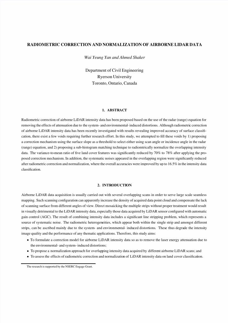
Fig. 1 show two sample areas located at the overlapping region of the two LiDAR data strips. The sub-figures (c) show the
original intensity (OI) image and the sub-figures (d) show the radiometrically corrected and normalized intensity (RCNI) image.
Systematic stripping noises were found on both OI images in vertical direction, where such noises were significantly reduced
in the RCNI images. We applied different classification scenarios on the first sample area in order to evaulate the impact of the
proposed approaches on land cover classification. The overall accuracy produced by the OI was close to 83%, where the RCNI
produced a slightly improved accuracy of 86.5%. Such increase was mainly due to the improvement of distinguishing Built-up
Land after radiometric correction and normalization, where both the ONI and the RCNI recorded a kappa statistics (KS) value
of 0.758 compared to 0.594 recorded in the results of the OI. In the 3-class scenario, the overall accuracy of the OI was 71.8%;
8% accuracy improvement was achieved in the classification results of RCNI. The KS value of the RCNI was found increased
by 0.1 in both High Rangeland and Low Rangeland. In the 4-class and 5-class scenarios, the overall accuracy dropped to
63.5% and 45.1%. Nevertheless, an increase of the overall accuracy was found in all the normalized intensity data classification
results. Respective increases of 13.4% and 16.5% were observed in the 4-class scenario and 5-class scenario, respectively. The
KS value of Tree, Grass, Soil and Built-up Land were found with an increase from 0.08 to 0.22 in the the RCNI classification
results when compared to the corresponding KS values generated from the OI.
7/24/2019 Radiometric Correction and Normalization of Airborne Lidar Data
http://slidepdf.com/reader/full/radiometric-correction-and-normalization-of-airborne-lidar-data 4/4
(a)
(b) (c) (d)
(e)
(f)
(g)
(h)
Fig. 1. (a) Aerial Photo, (b) DSM (c) OI and (d) RCNI in an area located at the overlapping region
5. CONCLUSION
We presented an improved radiometric correction and a radiometric normalization model to remove the line strpping problem
in overlapping region for airborne LiDAR intensity data. The correction model utilizes the slope as a threshold to control
either using the scan angle or the incidence angle in the radar (range) equation for airborne LiDAR intensity data, and the
normalization model relies on the sub-histogram matching technique to normalize the intensity data in overlapping region. It
was found that the vmr was signficantly reduced by 70% to 78% of five different land cover features (building, grass, road, soil
and tree). An increase of the overall accuracy was found in between 5.7% and 16.5% (excluding the 2-class scenario) in the
classification results of RCNI. With the justification of different statistical assessments in this study, the proposed radiometriccorrection and normalization can significantly reduce the within-class variation and between-class confusion of the land cover
features, as well as reducing the line-stripping noise in the overlapping region. Although the proposed approaches demonstrates
a significant improvement in land cover homogeneity and classification, a universal laser reflection model is still desired for the
up-coming multispectral LiDAR sensors.
6. REFERENCES
[1] Jelalian A.V., Laser Radar Systems, Artech House, Boston, London, 1992.
[2] Hofle B. and Pfeifer N., “Correction of laser scanning intensity data: data and model-driven approaches,” ISPRS Journal
of Photogrammetry and Remote Sensing, vol. 62, no. 6, pp. 415–433, 2003.
[3] Soenen S.A., Peddle D.R., and Coburn C.A., “SCS+C: A modified sun-canopy-sensor topographic correction in forested
terrain,” IEEE Transactions on Geoscience and Remote Sensing, vol. 43, no. 9, pp. 2148–2159, 2005.
[4] Shaker A., Yan W.Y., and El-Ashmawy N., “The effects of laser reflection angle on radiometric correction of the airborne
LiDAR intensity data,” in ISPRS Workshop Laser Scanning 2011, Calgary, Canada, August 29-31 2011.
[5] Richter R., Kellenberger T., and Kaufmann H., “Comparison of topographic correction methods,” Remote Sensing, vol. 1,
pp. 184–196, 2009.


