1
Random Coupling Model: Statistical Predictions of
Interference in Complex Enclosures
Steven M. Anlage
with Bo Xiao, Edward Ott, Thomas Antonsen
Research funded by AFOSR and ONR
COST Action IC1407 (ACCREDIT)
University of Nottingham
4 April, 2016
2
The Maryland Wave Chaos Group
Tom Antonsen Steve AnlageEd Ott
Jen-Hao YehLPS
James HartLincoln Labs
Biniyam TaddeseFDA
Also:Undergraduate StudentsEliot BradshawJohn AbrahamsGemstone Team TESLA
Post-DocsGabriele GradoniMathew Frazier
NRL Collaborators: Tim Andreadis, Lou Pecora, Hai Tran, Sun Hong, Zach Drikas, Jesus Gil Gil
Funding: ONR, AFOSR, DURIP
John RodgersNRL, Naval Academy,
UMD
Ming-Jer LeeWorld Bank
Trystan Koch
Faculty
Graduate Students (current + former)
Mark HerreraHeron Systems
Bo Xiao Bisrat Addissie
3
Outline
• The Problem: Electromagnetic Interference
• Our Approach – A Wave Chaos Statistical Description
• The Random Coupling Model (RCM)
• Examples of the RCM in Practice
• Conclusions
4
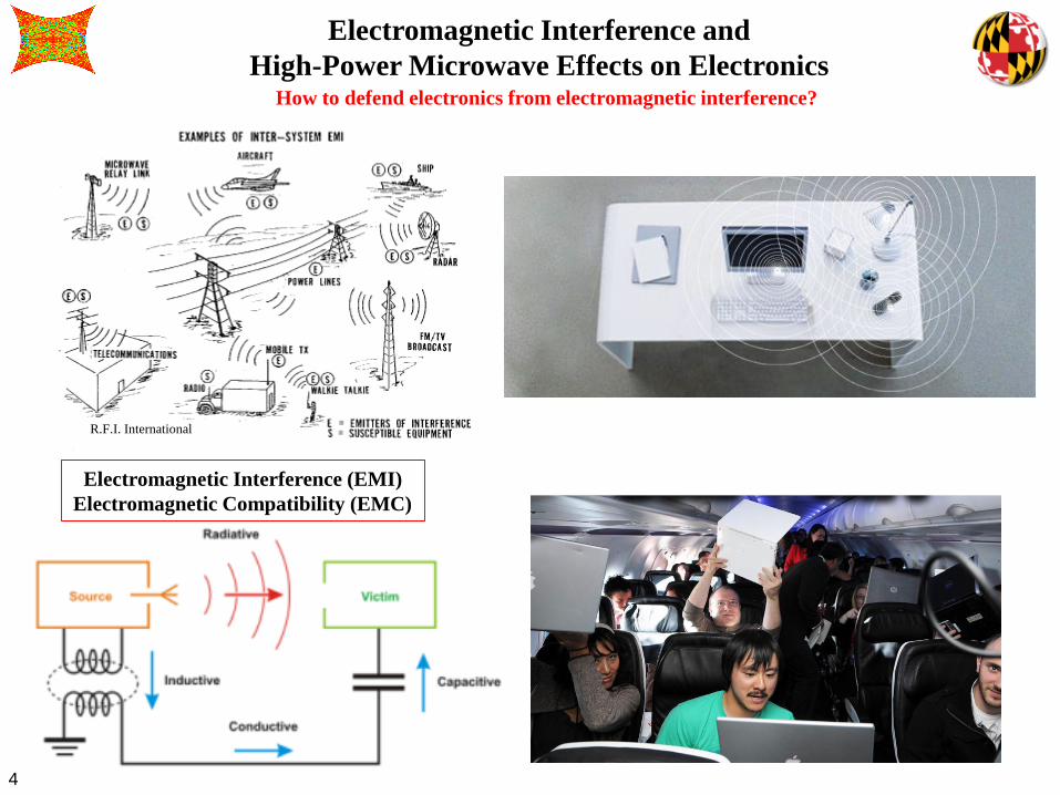
Electromagnetic Interference and
High-Power Microwave Effects on ElectronicsHow to defend electronics from electromagnetic interference?
R.F.I. International
Electromagnetic Interference (EMI)
Electromagnetic Compatibility (EMC)
5
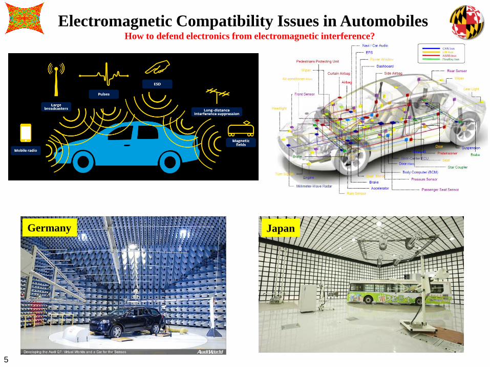
Electromagnetic Compatibility Issues in Automobiles
Germany Japan
How to defend electronics from electromagnetic interference?
6
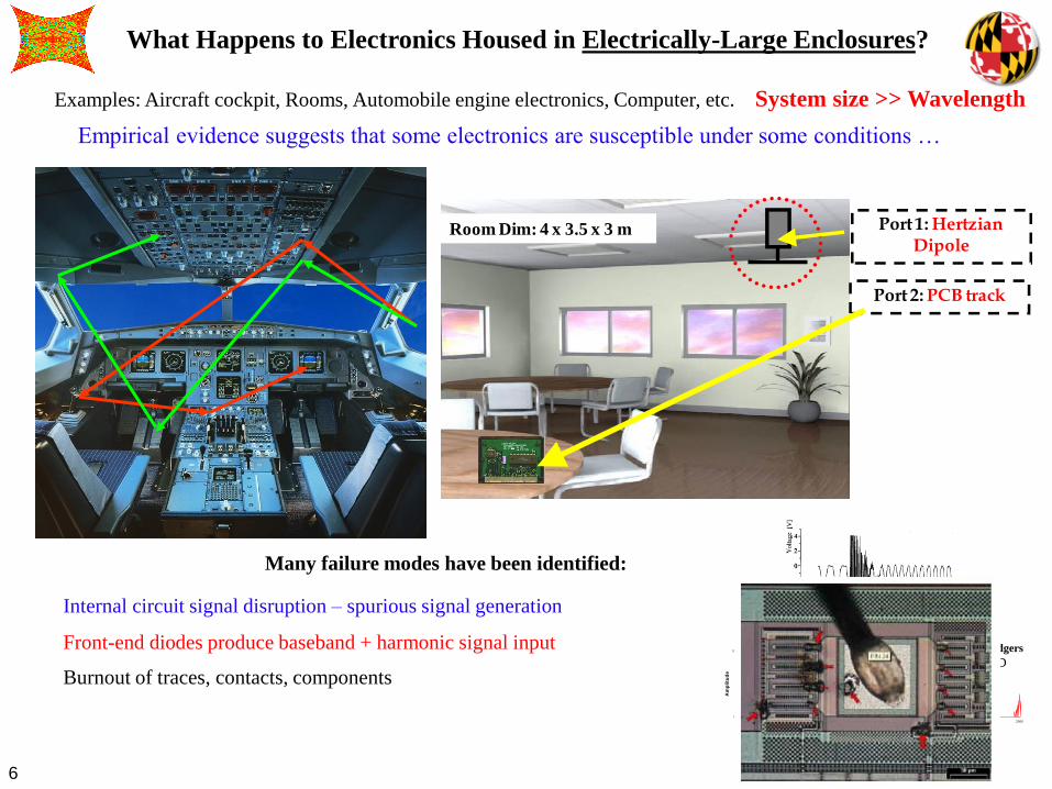
What Happens to Electronics Housed in Electrically-Large Enclosures?
Examples: Aircraft cockpit, Rooms, Automobile engine electronics, Computer, etc. System size >> Wavelength
Empirical evidence suggests that some electronics are susceptible under some conditions …
Many failure modes have been identified:
Internal circuit signal disruption – spurious signal generation
Front-end diodes produce baseband + harmonic signal input
Burnout of traces, contacts, components
0
10
0 2000
FrequencyA
mp
litu
de
0
10
0 2000
Frequency
Am
pli
tud
e
HPMJohn Rodgers
F. Sonnemann, Diehl
UMD
Room Dim: 4 x 3.5 x 3 m Port 1: Hertzian Dipole
Port 2: PCB track
7
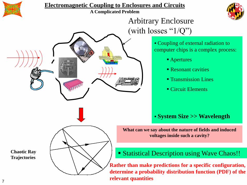
Electromagnetic Coupling to Enclosures and CircuitsA Complicated Problem
Coupling of external radiation to
computer chips is a complex process:
Apertures
Resonant cavities
Transmission Lines
Circuit Elements
System Size >> Wavelength
Chaotic Ray
Trajectories
What can we say about the nature of fields and induced
voltages inside such a cavity?
Statistical Description using Wave Chaos!!
Arbitrary Enclosure
(with losses “1/Q”)
Rather than make predictions for a specific configuration,
determine a probability distribution function (PDF) of the
relevant quantities
8
Outline
• The Problem: Electromagnetic Interference
• Our Approach – A Wave Chaos Statistical Description
• The Random Coupling Model (RCM)
• Examples of the RCM in Practice
• Conclusions

9
It makes no sense to talk about
“diverging trajectories” for waves
1) Waves do not have trajectories
Wave Chaos?
2) Linear wave systems can’t be chaotic
3) However in the semiclassical limit, you can think about rays
Wave Chaos concerns solutions of linear wave equations which,
in the semiclassical limit, can be described by chaotic ray trajectories
In the ray-limit
it is possible to define chaos
“ray chaos”
Maxwell’s equations, Schrödinger’s equation are linear

10
From Classical to Wave Chaos
wave
ray
trajectory
Quantum
Classical
(chaos)
Semiclassical limit
(quantum chaos)

11
H
Random Matrix Theory (RMT) and Wave ChaosWigner; Dyson; Mehta; Bohigas …
The RMT Approach:
Complicated Hamiltonian: e.g. Nucleus: Solve
Replace with a Hamiltonian with matrix elements chosen randomly
from a Gaussian distribution
Examine the statistical properties of the resulting Hamiltonians
This hypothesis has been tested in many systems:
Nuclei, atoms, molecules, quantum dots, acoustics (room, solid body, seismic),
optical resonators, random lasers,…
Some Questions:
Is this hypothesis supported by data in other systems?
What new applications are enabled by wave chaos?Can losses / decoherence be included?
What causes deviations from RMT predictions?
Hypothesis: Complicated Quantum/Wave systems that have chaotic classical/ray
counterparts possess universal statistical properties described by
Random Matrix Theory (RMT) “BGS Conjecture”
Cassati, 1980
Bohigas, 1984
EH
Orthogonal (real matrix elements, b = 1)
Unitary (complex matrix elements, b = 2)
Symplectic (quaternion matrix elements, b = 4)Universality Classes of RMT:
12
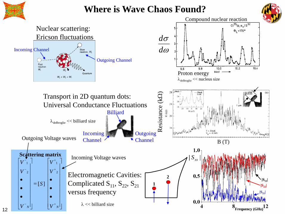
Where is Wave Chaos Found?
Billiard
Incoming
Channel
Outgoing
Channel
|S|S1111||
|S|S2222||
|S|S2121||
Frequency (GHz)
|| xxS
|S|S1111||
|S|S2222||
|S|S2121||
Frequency (GHz)
|| xxS
Electromagnetic Cavities:
Complicated S11, S22, S21
versus frequency
B (T)
Transport in 2D quantum dots:
Universal Conductance Fluctuations
Res
ista
nce
(k
W) mm
Nuclear scattering:
Ericson fluctuations
d
d
Proton energyldeBroglie << nucleus size
Compound nuclear reaction
1
2
Incoming Channel
Outgoing Channel
ldeBroglie << billiard size
l << billiard size
Incoming Voltage waves
Outgoing Voltage waves
S matrix
×
+
+
+
NN V
V
V
S
V
V
V
2
1
2
1
][
Scattering matrix
+
+
+
NN V
V
V
S
V
V
V
2
1
2
1
][
13
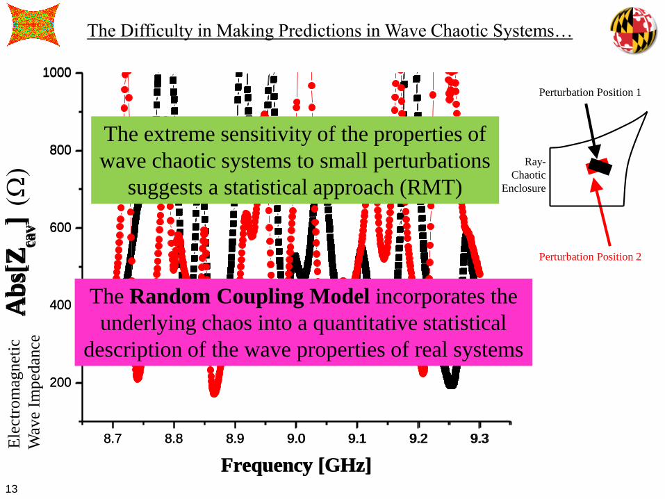
The Difficulty in Making Predictions in Wave Chaotic Systems…
8.7 8.8 8.9 9.0 9.1 9.2 9.3
200
400
600
800
1000
Ab
s[Z
cav]
Frequency [GHz]
Perturbation Position 1
8.7 8.8 8.9 9.0 9.1 9.2 9.3
200
400
600
800
1000
Ab
s[Z
cav]
Frequency [GHz]
Perturbation Position 2
(W)
Ele
ctro
mag
net
ic
Wav
e Im
ped
ance
The extreme sensitivity of the properties of
wave chaotic systems to small perturbations
suggests a statistical approach (RMT)
The Random Coupling Model incorporates the
underlying chaos into a quantitative statistical
description of the wave properties of real systems
Ray-
Chaotic
Enclosure
14
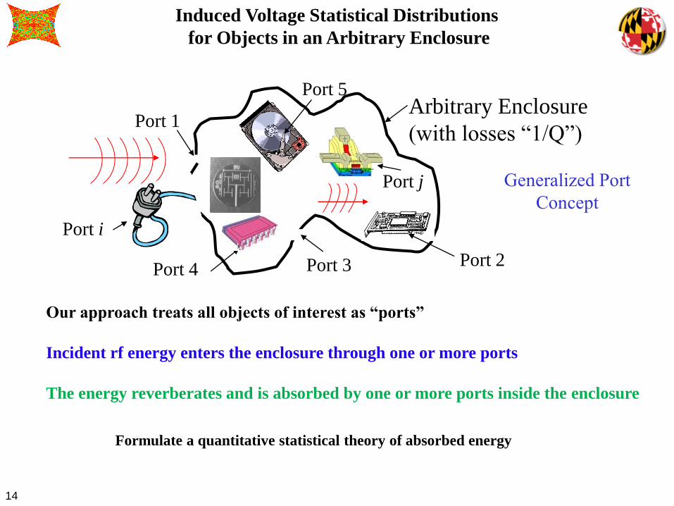
Induced Voltage Statistical Distributions
for Objects in an Arbitrary Enclosure
Arbitrary Enclosure
(with losses “1/Q”)Port 1
Port 2Port 3Port 4
Port 5
Generalized Port
Concept
Port i
Port j
Our approach treats all objects of interest as “ports”
Incident rf energy enters the enclosure through one or more ports
The energy reverberates and is absorbed by one or more ports inside the enclosure
Formulate a quantitative statistical theory of absorbed energy
15
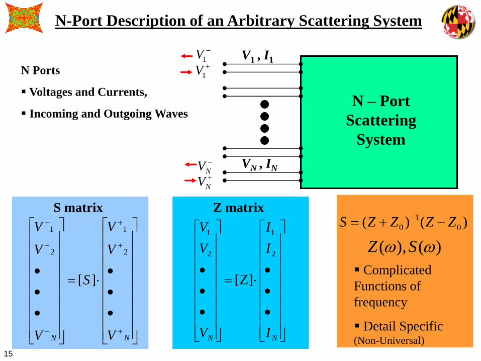
N-Port Description of an Arbitrary Scattering System
N – Port
Scattering
System
N Ports
Voltages and Currents,
Incoming and Outgoing Waves
Z matrixS matrix
1V+
1V
V1 , I1
VN , IN
NV+
NV
Complicated
Functions of
frequency
Detail Specific (Non-Universal)
)(),( SZ
)()( 0
1
0 ZZZZS +
+
+
+
NN V
V
V
S
V
V
V
2
1
2
1
][
NN I
I
I
V
V
V
2
1
2
1
][
16
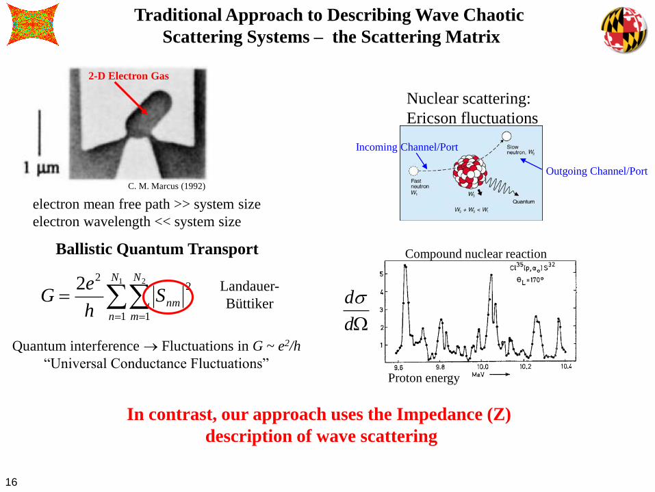
Traditional Approach to Describing Wave Chaotic
Scattering Systems – the Scattering Matrix
C. M. Marcus (1992)
2-D Electron Gas
electron mean free path >> system size
electron wavelength << system size
Ballistic Quantum Transport
Quantum interference Fluctuations in G ~ e2/h
“Universal Conductance Fluctuations”
Landauer-
Büttiker
1 2
1 1
222 N
n
N
m
nmSh
eG
Nuclear scattering:
Ericson fluctuations
Wd
d
Proton energy
Compound nuclear reaction
Incoming Channel/Port
Outgoing Channel/Port
In contrast, our approach uses the Impedance (Z)
description of wave scattering

17
Outline
• The Problem: Electromagnetic Interference
• Our Approach – A Wave Chaos Statistical Description
• The Random Coupling Model (RCM)
• Examples of the RCM in Practice
• Conclusions
18
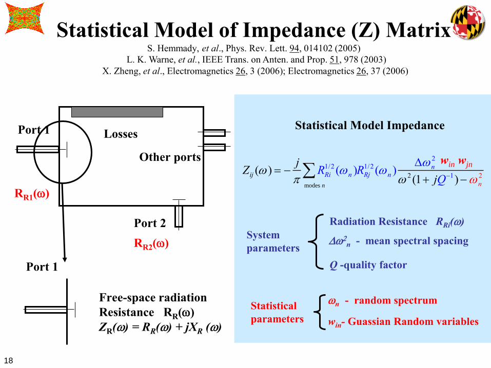
Statistical Model of Impedance (Z) MatrixS. Hemmady, et al., Phys. Rev. Lett. 94, 014102 (2005)
Port 1
Port 2
Other ports
Losses
Port 1
Free-space radiation
Resistance RR()
ZR() = RR() + jXR ()
RR1()
RR2()
Statistical Model Impedance
Q -quality factor
D2n - mean spectral spacing
Radiation Resistance RRi()
win- Guassian Random variables
n - random spectrum
System
parameters
Statistical
parameters
Zij ( ) j
RRi
1/2 (n )n
RRj1/2 (n )
Dn
2 winwin
2 (1+ jQ1) n
2
L. K. Warne, et al., IEEE Trans. on Anten. and Prop. 51, 978 (2003)
X. Zheng, et al., Electromagnetics 26, 3 (2006); Electromagnetics 26, 37 (2006)
modes n
win wjn
19
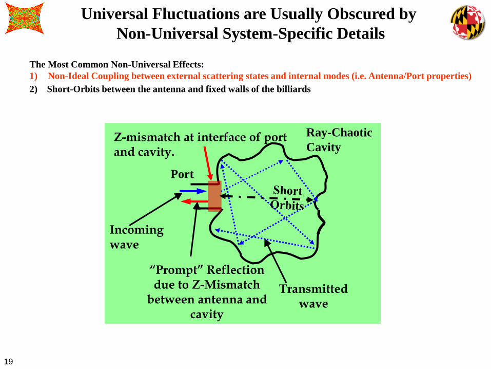
The Most Common Non-Universal Effects:
1) Non-Ideal Coupling between external scattering states and internal modes (i.e. Antenna/Port properties)
Universal Fluctuations are Usually Obscured by
Non-Universal System-Specific Details
Port
Ray-Chaotic
Cavity
Incoming wave
“Prompt” Reflection due to Z-Mismatch
between antenna and cavity
Z-mismatch at interface of port and cavity.
Transmitted wave
2) Short-Orbits between the antenna and fixed walls of the billiards

20
The Random Coupling ModelDivide and Conquer!
Enclosure Problem
Port 1
Port 2Port 3Port 4
Port 5
Port i
Port j
Coupling Problem
Mean
part
Fluctuating Part
(depends on a)
<Imx> = 1
<Rex > = 0
RadRad RiiXZZZ x++~
Solution: Random Matrix Theory;
Electromagnetic statistical properties are
governed by Loss Parameter a k2/(Dkn2 Q) df3dB/Dfspacing
Solution: Radiation Impedance Matrix Zrad
+ Short Orbits
Electromagnetics 26, 3 (2006)Electromagnetics 26, 37 (2006)Phys. Rev. Lett. 94, 014102 (2005)
Z matrix
NN I
I
I
V
V
V
2
1
2
1
][
IEEE Trans. EMC 54, 758 (2012)
21
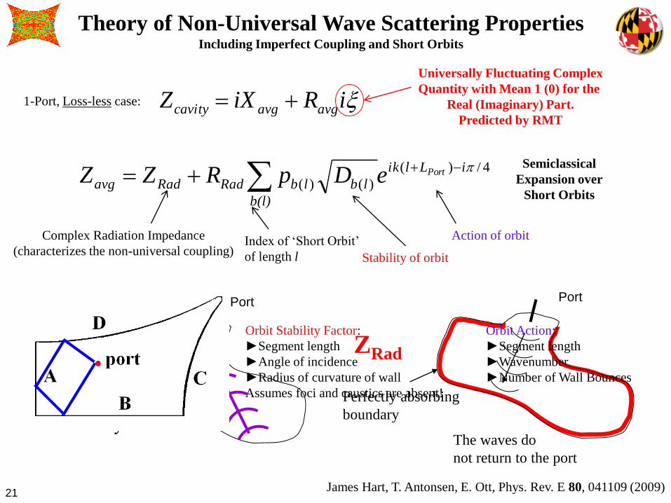
xiRiXZ avgavgcavity +
Universally Fluctuating Complex
Quantity with Mean 1 (0) for the
Real (Imaginary) Part.
Predicted by RMT
Semiclassical
Expansion over
Short Orbits
Complex Radiation Impedance
(characterizes the non-universal coupling)Index of ‘Short Orbit’
of length l Stability of orbit
Action of orbit
Theory of Non-Universal Wave Scattering PropertiesIncluding Imperfect Coupling and Short Orbits
James Hart, T. Antonsen, E. Ott, Phys. Rev. E 80, 041109 (2009)
Port
Zcavity
Port
ZRad
The waves do
not return to the port
Perfectly absorbing
boundaryCavity
Orbit Stability Factor:
►Segment length
►Angle of incidence
►Radius of curvature of wall
Assumes foci and caustics are absent!
Orbit Action:
►Segment length
►Wavenumber
►Number of Wall Bounces
1-Port, Loss-less case:
+
+b(l)
iLlik
lblbRadRadavgPorteDpRZZ
4/)(
)()(

22
8
0 1 20
1
2
3
-1 0 10
1
2
3
]ˆRe[ zl
])ˆ(Re[ zP l ])ˆ(Im[ zP l
]ˆIm[ zl
16a
3.6a
9.1a
16a
3.6a
9.1a
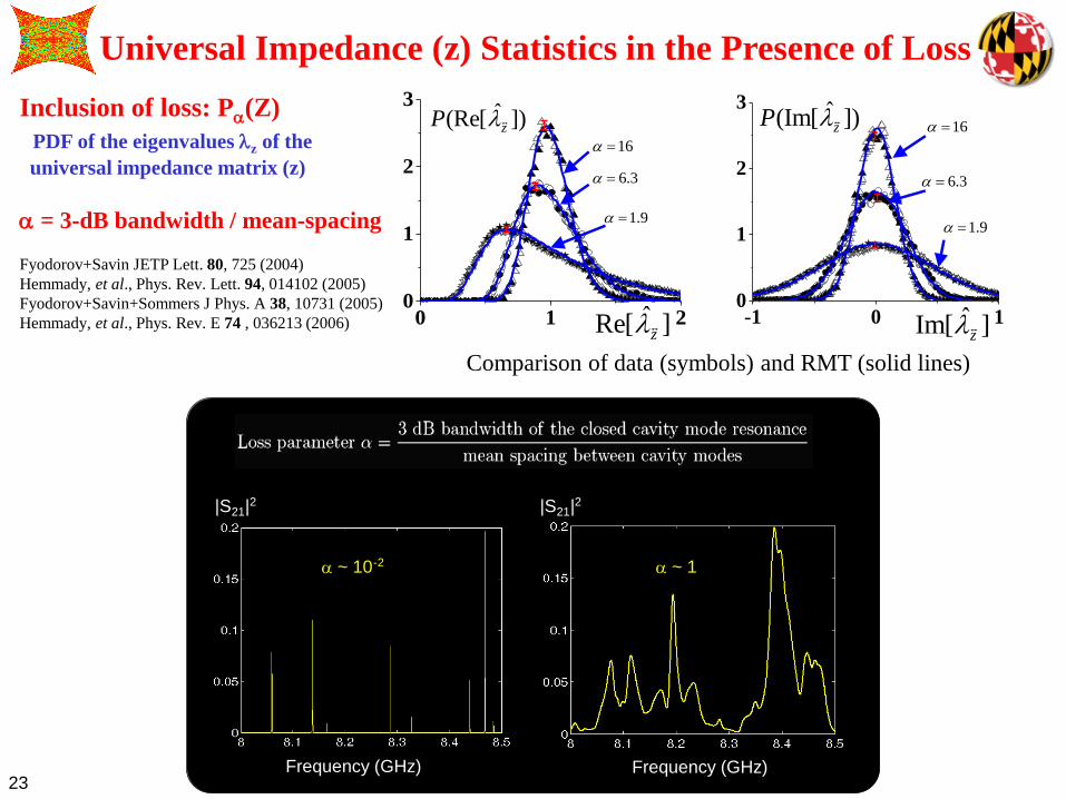
Inclusion of loss: Pa(Z)
a = 3-dB bandwidth / mean-spacing
Fyodorov+Savin JETP Lett. 80, 725 (2004)
Hemmady, et al., Phys. Rev. Lett. 94, 014102 (2005)
Fyodorov+Savin+Sommers J Phys. A 38, 10731 (2005)
Hemmady, et al., Phys. Rev. E 74 , 036213 (2006)
Mean of Pa(z)
Variance of Pa(z)
Universal Impedance (Z) Statistics in the Presence of Loss
a
1 1a
Comparison of data (symbols) and RMT (solid lines)
1ˆRe zE l 0ˆIm zE l Independent of a
23
8
0 1 20
1
2
3
-1 0 10
1
2
3
]ˆRe[ zl
])ˆ(Re[ zP l ])ˆ(Im[ zP l
]ˆIm[ zl
16a
3.6a
9.1a
16a
3.6a
9.1a
Inclusion of loss: Pa(Z)
PDF of the eigenvalues lz of the
universal impedance matrix (z)
Universal Impedance (z) Statistics in the Presence of Loss
a
1
Comparison of data (symbols) and RMT (solid lines)
1ˆRe zE l 0ˆIm zE l
a = 3-dB bandwidth / mean-spacing
Fyodorov+Savin JETP Lett. 80, 725 (2004)
Hemmady, et al., Phys. Rev. Lett. 94, 014102 (2005)
Fyodorov+Savin+Sommers J Phys. A 38, 10731 (2005)
Hemmady, et al., Phys. Rev. E 74 , 036213 (2006)
Frequency (GHz) Frequency (GHz)
|S21|2 |S21|2
a ~ 10-2 a ~ 1
24
Outline
• The Problem: Electromagnetic Interference
• Our Approach – A Wave Chaos Statistical Description
• The Random Coupling Model (RCM)
• Examples of the RCM in Practice
• Conclusions

25
Microwave Cavity Analog of a
2D Quantum Infinite Square Well
Table-top experiment!
Ez
Bx By
( )
boundariesatwith
VEm
n
nnn
0
02
2
2
+ Schrödinger equation
boundariesatEwith
EkE
nz
nznnz
0
0
,
,
2
,
2
+Helmholtz equation
Stöckmann + Stein, 1990
Doron+Smilansky+Frenkel, 1990
Sridhar, 1991
Richter, 1992
d ≈ 8 mm
An empty “two-dimensional” electromagnetic resonator
Bow-Tie Billiard
A. Gokirmak, et al. Rev. Sci. Instrum. 69, 3410 (1998)
~ 50 cm
The only propagating
mode for f < c/d:Metal walls
26
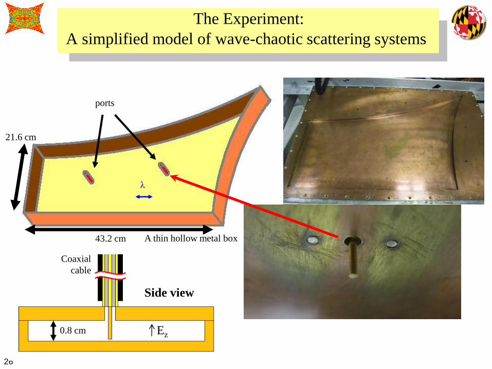
The Experiment:
A simplified model of wave-chaotic scattering systems
A thin hollow metal box
ports
Side view
21.6 cm
43.2 cm
0.8 cm
λ
Ez
Coaxial
cable
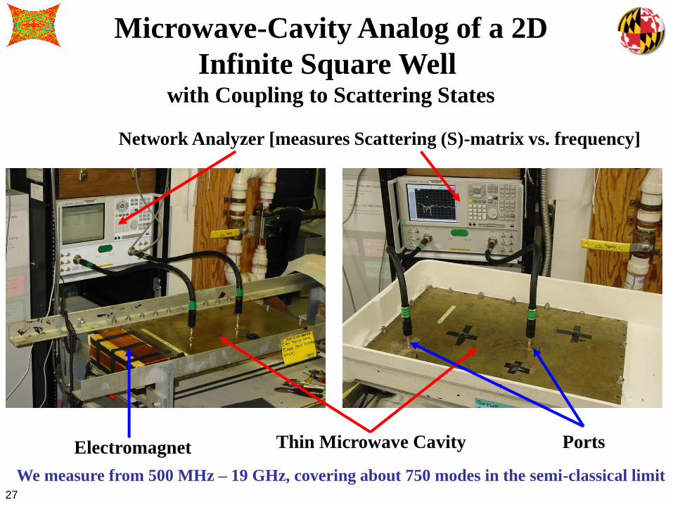
27
Microwave-Cavity Analog of a 2D
Infinite Square Well with Coupling to Scattering States
Network Analyzer [measures Scattering (S)-matrix vs. frequency]
Thin Microwave Cavity PortsElectromagnet
We measure from 500 MHz – 19 GHz, covering about 750 modes in the semi-classical limit
28
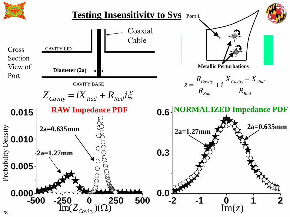
Pro
bab
ilit
y D
ensi
ty
-2 -1 0 1 20.0
0.3
0.6
2a=0.635mm2a=1.27mm
)Im(z-500 -250 0 250 500
0.000
0.005
0.010
0.015
2a=1.27mm
2a=0.635mm
))(Im( WCavityZ
Testing Insensitivity to System Details
CAVITY BASE
Cross
Section
View of
Port
CAVITY LID
Diameter (2a)
Coaxial
Cable Freq. Range : 9 to 9.75 GHz
Cavity Height : h= 7.87mm
Statistics drawn from 100,125 pts.
Rad
RadCavity
Rad
Cavity
R
XXi
R
Rz
+
RAW Impedance PDF NORMALIZED Impedance PDF
Metallic Perturbations
Port 1
xiRiXZ RadRadCavity +
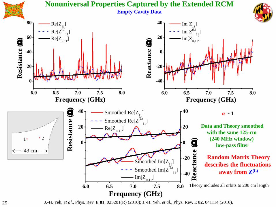
29
Data and Theory smoothed
with the same 125-cm
(240 MHz window)
low-pass filter
Nonuniversal Properties Captured by the Extended RCMEmpty Cavity Data
Theory includes all orbits to 200 cm length
6.0 6.5 7.0 7.5 8.0
0
20
40
60
80R
esis
tan
ce (
W)
Frequency (GHz)
Re[Z11
]
Re[Z(L)
11]
Re[ZR,11
]
6.0 6.5 7.0 7.5 8.0
-40
-20
0
20
40
Rea
ctan
ce (
W)
Frequency (GHz)
Im[Z11
]
Im[Z(L)
11]
Im[ZR,11
]
6.0 6.5 7.0 7.5 8.0
-40
-20
0
20
40
-40
-20
0
20
40
R
eact
an
ce (
W)
Smoothed Im[Z11
]
Smoothed Im[Z(L)
11]
Im[ZR,11
]
Res
ista
nce
(W
)
Frequency (GHz)
Smoothed Re[Z11
]
Smoothed Re[Z(L)
11]
Re[ZR,11
]
J.-H. Yeh, et al., Phys. Rev. E 81, 025201(R) (2010); J.-H. Yeh, et al., Phys. Rev. E 82, 041114 (2010).
43 cm
Random Matrix Theory
describes the fluctuations
away from Z(L)
1 2
a ~ 1
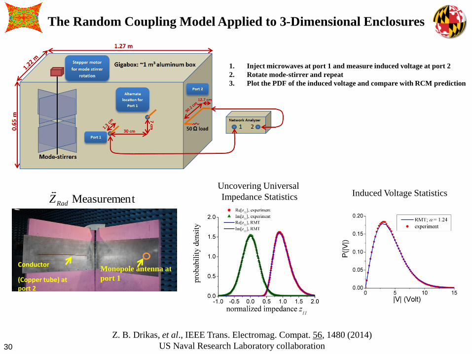
30
The Random Coupling Model Applied to 3-Dimensional Enclosures
Uncovering Universal
Impedance Statistics
Conductor
(Copper tube) at port 2
Monopole antenna at
port 1
tMeasuremen RadZ Induced Voltage Statistics
Z. B. Drikas, et al., IEEE Trans. Electromag. Compat. 56, 1480 (2014)
US Naval Research Laboratory collaboration
1. Inject microwaves at port 1 and measure induced voltage at port 2
2. Rotate mode-stirrer and repeat
3. Plot the PDF of the induced voltage and compare with RCM prediction
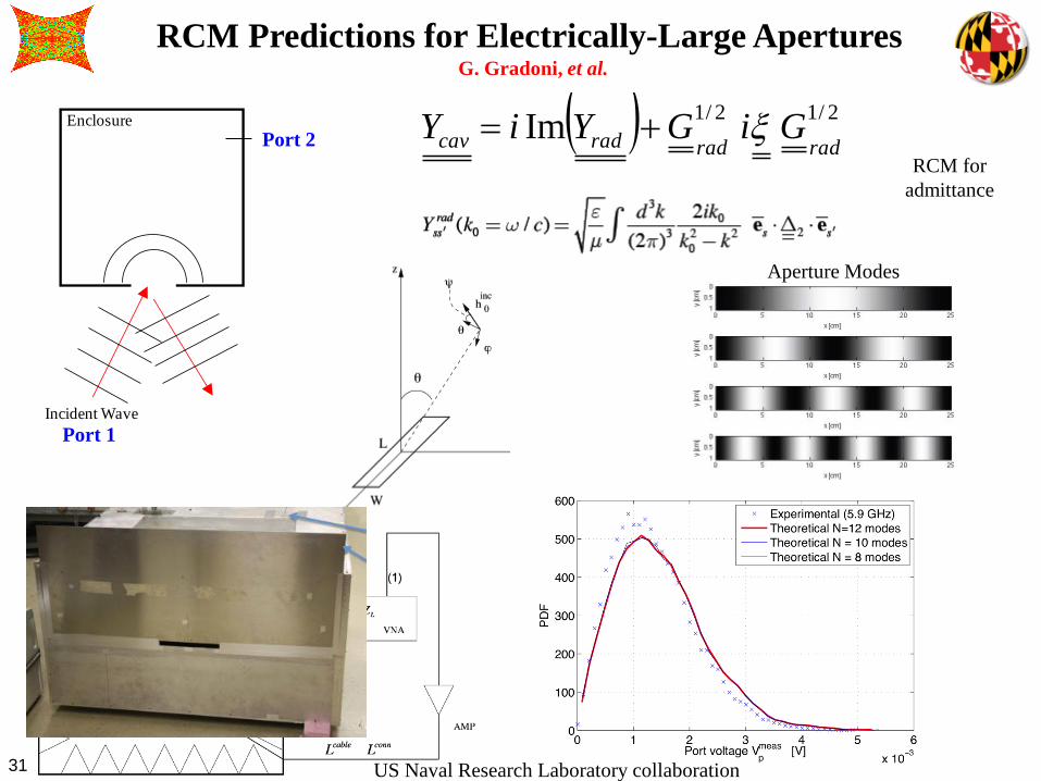
31
RCM Predictions for Electrically-Large AperturesG. Gradoni, et al.
Enclosure
Incident Wave
( ) 2/12/1Im
radradradcav GiGYiY x+RCM for
admittance
Port 2
Port 1
Aperture Modes
US Naval Research Laboratory collaboration
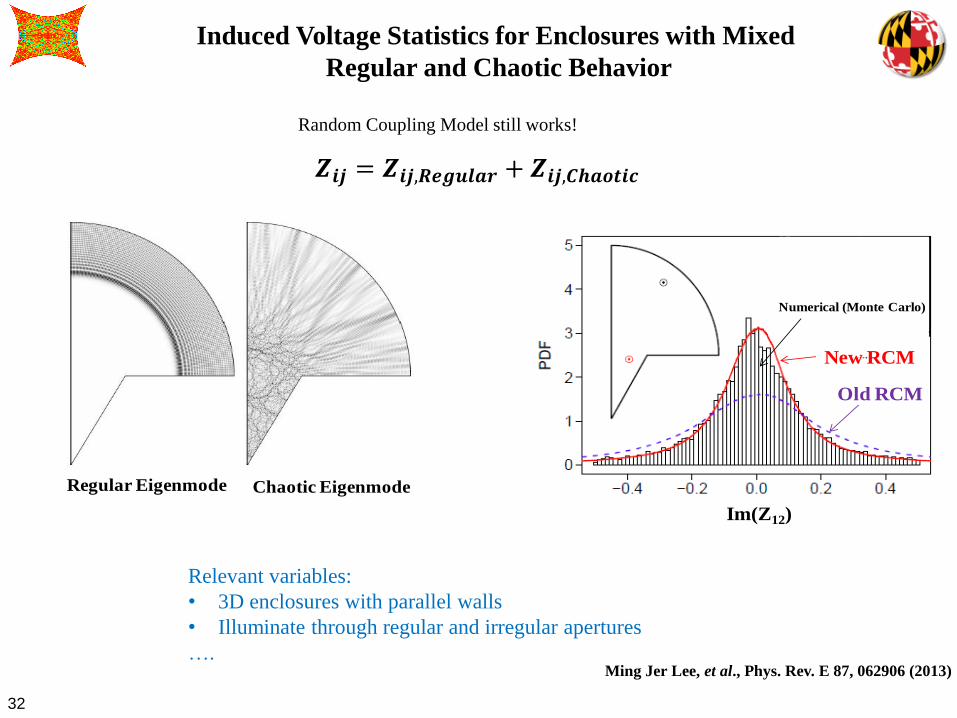
32
Induced Voltage Statistics for Enclosures with Mixed
Regular and Chaotic Behavior
Chaotic EigenmodeRegular Eigenmode
Im(Z12)
Old RCM
New RCM
Numerical (Monte Carlo)
Relevant variables:
• 3D enclosures with parallel walls
• Illuminate through regular and irregular apertures
….Ming Jer Lee, et al., Phys. Rev. E 87, 062906 (2013)
Random Coupling Model still works!
𝒁𝒊𝒋 = 𝒁𝒊𝒋,𝑹𝒆𝒈𝒖𝒍𝒂𝒓 + 𝒁𝒊𝒋,𝑪𝒉𝒂𝒐𝒕𝒊𝒄

33
Outline
• The Problem: Electromagnetic Interference
• Our Approach – A Wave Chaos Statistical Description
• The Random Coupling Model (RCM)
• Examples of the RCM in Practice
• Related Work
• Conclusions
34
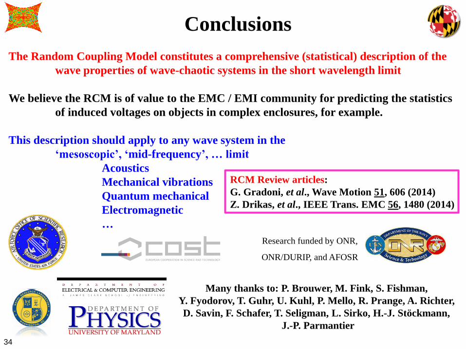
Conclusions
Many thanks to: P. Brouwer, M. Fink, S. Fishman,
Y. Fyodorov, T. Guhr, U. Kuhl, P. Mello, R. Prange, A. Richter,
D. Savin, F. Schafer, T. Seligman, L. Sirko, H.-J. Stöckmann,
J.-P. Parmantier
The Random Coupling Model constitutes a comprehensive (statistical) description of the
wave properties of wave-chaotic systems in the short wavelength limit
We believe the RCM is of value to the EMC / EMI community for predicting the statistics
of induced voltages on objects in complex enclosures, for example.
This description should apply to any wave system in the
‘mesoscopic’, ‘mid-frequency’, … limit
Acoustics
Mechanical vibrations
Quantum mechanical
Electromagnetic
…
RCM Review articles:
G. Gradoni, et al., Wave Motion 51, 606 (2014)
Z. Drikas, et al., IEEE Trans. EMC 56, 1480 (2014)
Research funded by ONR,
ONR/DURIP, and AFOSR
35
Students and Post-docs
• Present Students Wave Chaos
• Recent Post-docs
Gabriele Gradoni,
U. Nottingham, UK
Trystan Koch Bisrat AddissieBo Xiao
Faranstul Adnan Ke Ma Ziyuan Fu
Min Zhou Alan Liu


