
Recent Developments in Panel Models for Count Data
Pravin K. TrivediIndiana University. - Bloomington
Prepared for 2010 Mexican Stata Users Group meeting,based on
A. Colin Cameron and Pravin K. Trivedi (2005),Microeconometrics: Methods and Applications (MMA), C.U.P.
MMA, chapters 21-23and
A. Colin Cameron and Pravin K. Trivedi (2010),Microeconometrics using Stata Revised edition (MUSR), Stata Press.
MUSR, chapters 8;18.
April 29, 2010
Pravin K. Trivedi Indiana University. - Bloomington (Prepared for 2010 Mexican Stata Users Group meeting, based on A. Colin Cameron and Pravin K. Trivedi (2005), Microeconometrics: Methods and Applications (MMA), C.U.P. MMA, chapters 21-23 and A. Colin Cameron and Pravin K. Trivedi (2010), Microeconometrics using Stata Revised edition (MUSR), Stata Press. MUSR, chapters 8;18. )Panel counts April 29, 2010 1 / 77

Introduction
0. Dedication
Pravin K. Trivedi Indiana University. - Bloomington (Prepared for 2010 Mexican Stata Users Group meeting, based on A. Colin Cameron and Pravin K. Trivedi (2005), Microeconometrics: Methods and Applications (MMA), C.U.P. MMA, chapters 21-23 and A. Colin Cameron and Pravin K. Trivedi (2010), Microeconometrics using Stata Revised edition (MUSR), Stata Press. MUSR, chapters 8;18. )Panel counts April 29, 2010 2 / 77

Introduction
1. Introduction
Objective 1: To survey recent developments in count data panelmodels
Objective 2: Evaluate the advances made against background of mainfeatures of count data
Objective 3: Highlight the areas where signicant gaps exist andreview the most promising approaches
Pravin K. Trivedi Indiana University. - Bloomington (Prepared for 2010 Mexican Stata Users Group meeting, based on A. Colin Cameron and Pravin K. Trivedi (2005), Microeconometrics: Methods and Applications (MMA), C.U.P. MMA, chapters 21-23 and A. Colin Cameron and Pravin K. Trivedi (2010), Microeconometrics using Stata Revised edition (MUSR), Stata Press. MUSR, chapters 8;18. )Panel counts April 29, 2010 3 / 77

Introduction
Background (1)Panel data are repeated measures on individuals (i) over time (t):data are (yit , xit ) for i = 1, ...,N and t = 1, ...,T , and yit arenonnegative integer-valued outcomes.Conditional on xit , the yit are likely to be serially correlated for agiven i , partly because of state dependence and partly because ofcserial correlation in shocks.Hence each additional year of data is not independent of previousyears.Cross-sectional dependence between observations is also to beexpected given emphasis on stratied clustered sampling designs.(1) Pervasive unobserved heterogeneity, (2) a typically highproportion of zeros, (3) inherent discreteness and heteroskedasticitygenerate complications that are hard to handle simultaneouslyFinally, the researchers interest often goes beyond the conditionalmean.How well does available software (Stata) handle these issues?
Pravin K. Trivedi Indiana University. - Bloomington (Prepared for 2010 Mexican Stata Users Group meeting, based on A. Colin Cameron and Pravin K. Trivedi (2005), Microeconometrics: Methods and Applications (MMA), C.U.P. MMA, chapters 21-23 and A. Colin Cameron and Pravin K. Trivedi (2010), Microeconometrics using Stata Revised edition (MUSR), Stata Press. MUSR, chapters 8;18. )Panel counts April 29, 2010 4 / 77

Introduction Basic linear panel models
2. Basic linear panel models review
Pooled model (or population-averaged)
yit = α+ x0itβ+ uit . (1)
Two-way e¤ects model allows intercept to vary over i and t
yit = αi + γt + x0itβ+ εit . (2)
Individual-specic e¤ects model
yit = αi + x0itβ+ εit , (3)
where αi may be xed e¤ect or random e¤ect.
Mixed model or random coe¢ cients model allows slopes to vary over i
yit = αi + x0itβi + εit . (4)
Pravin K. Trivedi Indiana University. - Bloomington (Prepared for 2010 Mexican Stata Users Group meeting, based on A. Colin Cameron and Pravin K. Trivedi (2005), Microeconometrics: Methods and Applications (MMA), C.U.P. MMA, chapters 21-23 and A. Colin Cameron and Pravin K. Trivedi (2010), Microeconometrics using Stata Revised edition (MUSR), Stata Press. MUSR, chapters 8;18. )Panel counts April 29, 2010 5 / 77

Introduction Fixed versus random e¤ects model
3. Fixed e¤ects versus random e¤ects model
Individual-specic e¤ects model:
yit = x0itβ+ (αi + εit ).
Fixed e¤ects (FE):I αi is a random variable possibly correlated with xitI so regressor xit may be endogenous (wrt to αi but not εit )e.g. education is correlated with time-invariant ability
I pooled OLS, pooled GLS, RE are inconsistent for βI within (FE) and rst di¤erence estimators are consistent.
Random e¤ects (RE) or population-averaged (PA):I αi is purely random (usually iid (0, σ2α)) unrelated to xitI so regressor xit is exogenousI appropraite FE and RE estimators are consistent for β
Fundamental divide: microeconometricians FE versus others RE.
Pravin K. Trivedi Indiana University. - Bloomington (Prepared for 2010 Mexican Stata Users Group meeting, based on A. Colin Cameron and Pravin K. Trivedi (2005), Microeconometrics: Methods and Applications (MMA), C.U.P. MMA, chapters 21-23 and A. Colin Cameron and Pravin K. Trivedi (2010), Microeconometrics using Stata Revised edition (MUSR), Stata Press. MUSR, chapters 8;18. )Panel counts April 29, 2010 6 / 77

Nonlinear panel models Overview
4. Some features of nonlinear panel models
In contrast to linear models, solutions for nonlinear models tend tolack generality and are model-specic.
Standard count models include: Poisson and negative binomial
General approaches are similar to those for the linear caseI Pooled estimation or population-averagedI Random e¤ectsI Fixed e¤ects
ComplicationsI Random e¤ects often not tractable so need numerical integrationI Fixed e¤ects models in short panels are generally not estimable due tothe incidental parameters problem.
I Count models involve discreteness, nonlinearity and intrinsicheteroskedasticity.
Pravin K. Trivedi Indiana University. - Bloomington (Prepared for 2010 Mexican Stata Users Group meeting, based on A. Colin Cameron and Pravin K. Trivedi (2005), Microeconometrics: Methods and Applications (MMA), C.U.P. MMA, chapters 21-23 and A. Colin Cameron and Pravin K. Trivedi (2010), Microeconometrics using Stata Revised edition (MUSR), Stata Press. MUSR, chapters 8;18. )Panel counts April 29, 2010 7 / 77

Nonlinear panel models Overview
Some Standard Cross-section Count Models
f (y ) f (y ) = Pr[Y = y ] Mean; Variance
1 Poisson eµµy/y ! µ(x); µ(x) = exp(x0β)2 NB1 As in NB2 below with α1 replaced by α1µ µ(x); (1+ α) µ(x)
3 NB2Γ(α1 + y )
Γ(α1)Γ(y + 1)
α1
α1 + µ
1α
µ
µ+ α1
yµ(x) ; (1+ αµ(x)) µ(x)
4 Hurdle
8<: f1(0) if y = 0,1 f1(0)1 f2(0)
f2(y ) if y 1. Pr[y > 0jx]Ey>0 [y jy > 0, x];
5 ZIf1(0) + (1 f1(0))f2(0) if y = 0,
(1 f1(0))f2(y ) if y 1. (1 f1(0))
(µ(x)+f1(0)µ2(x))6 FMM ∑mj=1 πj fj (y jθj ) Σ2i=1πiµi (x);
Σ2i=1πi [µi (x) + µ2i (x)]
Pravin K. Trivedi Indiana University. - Bloomington (Prepared for 2010 Mexican Stata Users Group meeting, based on A. Colin Cameron and Pravin K. Trivedi (2005), Microeconometrics: Methods and Applications (MMA), C.U.P. MMA, chapters 21-23 and A. Colin Cameron and Pravin K. Trivedi (2010), Microeconometrics using Stata Revised edition (MUSR), Stata Press. MUSR, chapters 8;18. )Panel counts April 29, 2010 8 / 77
Nonlinear panel models Overview
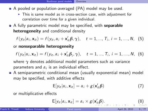
A pooled or population-averaged (PA) model may be used.I This is same model as in cross-section case, with adjustment forcorrelation over time for a given individual.
A fully parametric model may be specied, with separableheterogeneity and conditional density
f (yit jαi , xit ) = f (yit , αi + x0itβ,γ), t = 1, ...,Ti , i = 1, ....,N, (5)
or nonseparable heterogeneity
f (yit jαi , xit ) = f (yit , αi + x0itβi ,γ), t = 1, ...,Ti , i = 1, ....,N, (6)
where γ denotes additional model parameters such as varianceparameters and αi is an individual e¤ect.A semiparametric conditional mean (usually exponential mean) modelmay be specied, with additive e¤ects
E[yit jαi , xit ] = αi + g(x0itβ) (7)
or multiplicative e¤ects
E[yit jαi , xit ] = αi g(x0itβ). (8)
Pravin K. Trivedi Indiana University. - Bloomington (Prepared for 2010 Mexican Stata Users Group meeting, based on A. Colin Cameron and Pravin K. Trivedi (2005), Microeconometrics: Methods and Applications (MMA), C.U.P. MMA, chapters 21-23 and A. Colin Cameron and Pravin K. Trivedi (2010), Microeconometrics using Stata Revised edition (MUSR), Stata Press. MUSR, chapters 8;18. )Panel counts April 29, 2010 9 / 77

Nonlinear panel models Overview
5. Evolution of Panel Models (1)
Focus on panel methods most commonly used bymicroeconometricians. The underlying asymptotic theory assumesshort panels (T small, N large): data on many individual units andfew time periods.
The key paper in the modern treatment of panel analysis for counts isHausman et al. (1984).
The developments since 1984 can be summarized in generationalterms as follows.
Pravin K. Trivedi Indiana University. - Bloomington (Prepared for 2010 Mexican Stata Users Group meeting, based on A. Colin Cameron and Pravin K. Trivedi (2005), Microeconometrics: Methods and Applications (MMA), C.U.P. MMA, chapters 21-23 and A. Colin Cameron and Pravin K. Trivedi (2010), Microeconometrics using Stata Revised edition (MUSR), Stata Press. MUSR, chapters 8;18. )Panel counts April 29, 2010 10 / 77

Nonlinear panel models Overview
Evolution of Panel Models (2)
G-1 models G-2 models G-3 models
Period 1974-1990 1991-2000 Post-2000
Function Mainly parametric Flexible parametric Parametric / SP
CS models Poisson, Negbin Hurdles, nite Quantile reg;
mixtures, ZIP Selection models
Panel models Poisson, Negbin Poisson, Negbin, EM EM; QR;
Unobs. hetero. Multiplicative Separable or nonsep. Flexible; non-sep
Modeling αi Mainly RE or PA RE, PA and RE/PA/FE/
xed e¤ects Correlated RE; DV
Variance est. Robust Robust Robust or Cl-Rob
wrt overdispersion wrt OD wrt OD/SC
Dynamics Lagged xs Exponential feedback Linear or exponential
Endogeneity Largely ignored Allowed in RE models Allowed in RE and FE
Estimators Mainly MLE MLE; GEE; NLIV; MLE; GEE; NLGMM;
QR; QRIV
Pravin K. Trivedi Indiana University. - Bloomington (Prepared for 2010 Mexican Stata Users Group meeting, based on A. Colin Cameron and Pravin K. Trivedi (2005), Microeconometrics: Methods and Applications (MMA), C.U.P. MMA, chapters 21-23 and A. Colin Cameron and Pravin K. Trivedi (2010), Microeconometrics using Stata Revised edition (MUSR), Stata Press. MUSR, chapters 8;18. )Panel counts April 29, 2010 11 / 77

Nonlinear panel models Overview
6. Remarks on the evolution of count panel models (2)
FE panel data counterparts of several popular cross-section modelslike hurdles, FMM, and ZIP are undeveloped.
When several complications occur simultaneously (e.g. nonseprableindividual-specic e¤ects and endogenous regressors) they are mostconveniently analyzed in a RE or PA or moment-based models.
Fully parametric methods for simultaneously handling endogeneityplus something else (e.g. nonseparable UH) are largely absent, andmoment-based methods are a dominant alternative.
Overdispersion-robust and cluster-robust estimation of variances isnow feasible and very common.
Pravin K. Trivedi Indiana University. - Bloomington (Prepared for 2010 Mexican Stata Users Group meeting, based on A. Colin Cameron and Pravin K. Trivedi (2005), Microeconometrics: Methods and Applications (MMA), C.U.P. MMA, chapters 21-23 and A. Colin Cameron and Pravin K. Trivedi (2010), Microeconometrics using Stata Revised edition (MUSR), Stata Press. MUSR, chapters 8;18. )Panel counts April 29, 2010 12 / 77

Nonlinear panel estimators Pooled or population-averaged estimators
7. Nonlinear: Pooled or population-averaged estimators
Extend pooled OLS to the nonlinear caseI Give the usual cross-section command for conditional mean models orconditional density models but then get cluster-robust standard errors
I Poisson example:poisson y x, vce(cluster id)orxtgee y x, fam(poisson) link(log) corr(ind) vce(clusterid)
Extend pooled feasible GLS to the nonlinear caseI Estimate with an assumed correlation structure over timeI Equicorrelated probit example:xtpoisson y x, pa vce(boot)orxtgee y x, fam(poisson) link(log) corr(exch) vce(clusterid)
Pravin K. Trivedi Indiana University. - Bloomington (Prepared for 2010 Mexican Stata Users Group meeting, based on A. Colin Cameron and Pravin K. Trivedi (2005), Microeconometrics: Methods and Applications (MMA), C.U.P. MMA, chapters 21-23 and A. Colin Cameron and Pravin K. Trivedi (2010), Microeconometrics using Stata Revised edition (MUSR), Stata Press. MUSR, chapters 8;18. )Panel counts April 29, 2010 13 / 77

Nonlinear panel estimators Random e¤ects estimators
Nonlinear random e¤ects estimatorsAssume individual-specic e¤ect αi has specied distribution g(αi jη).Then the unconditional density for the i th observation is
f (yit , ..., yiT jxi1, ..., xiT , β,γ, η)
=Z h
∏Tt=1 f (yit jxit , αi , β,γ)
ig(αi jη)dαi . (9)
Analytical solution:I For Poisson with gamma random e¤ectI For negative binomial with gamma e¤ectI Use xtpoisson, re and xtnbreg, re
No analytical solution:I For other models.I Instead use numerical integration (only univariate integration isrequired).
I Assume normally distributed random e¤ects.I Use re option for xtlogit, xtprobitI Use normal option for xtpoisson and xtnbreg
Pravin K. Trivedi Indiana University. - Bloomington (Prepared for 2010 Mexican Stata Users Group meeting, based on A. Colin Cameron and Pravin K. Trivedi (2005), Microeconometrics: Methods and Applications (MMA), C.U.P. MMA, chapters 21-23 and A. Colin Cameron and Pravin K. Trivedi (2010), Microeconometrics using Stata Revised edition (MUSR), Stata Press. MUSR, chapters 8;18. )Panel counts April 29, 2010 14 / 77
Nonlinear panel estimators Random slopes estimators
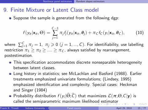
9. Finite Mixture or Latent Class modelSuppose the sample is generated from the following dgp:
f (yit jxit ,Θ) =C1∑j=1
πj fj (yit jxit , θj ) + πC fC (yi jxit , θC ), (10)
where ∑Cj=1 πj = 1, πj > 0 (j = 1, ...,C ). For identiability, use labelling
restriction π1 π2 .... πC , always satised by rearrangement,postestimation.
This specication accommodates discrete nonseparable heterogeneitybetween latent classes.Long history in statistics; see McLachlan and Basford (1988). Earliertreatments emphasized univariate formulations; (Lindsey, 1995)emphasized identication and complexity. Special cases: Heckmanand Singer (1984)Probability distribution f (yi jbΘ;bC ) that maximizes L(π,Θ,C jy) iscalled the semiparametric maximum likelihood estimator
Pravin K. Trivedi Indiana University. - Bloomington (Prepared for 2010 Mexican Stata Users Group meeting, based on A. Colin Cameron and Pravin K. Trivedi (2005), Microeconometrics: Methods and Applications (MMA), C.U.P. MMA, chapters 21-23 and A. Colin Cameron and Pravin K. Trivedi (2010), Microeconometrics using Stata Revised edition (MUSR), Stata Press. MUSR, chapters 8;18. )Panel counts April 29, 2010 15 / 77
Nonlinear panel estimators Random slopes estimators
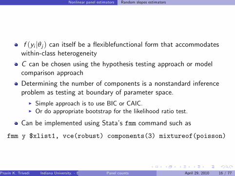
f (yi jθj ) can itself be a exiblefunctional form that accommodateswithin-class heterogeneity
C can be chosen using the hypothesis testing approach or modelcomparison approach
Determining the number of components is a nonstandard inferenceproblem as testing at boundary of parameter space.
I Simple approach is to use BIC or CAIC.I Or do appropriate bootstrap for the likelihood ratio test.
Can be implemented using Statas fmm command such as
fmm y $xlist1, vce(robust) components(3) mixtureof(poisson)
Pravin K. Trivedi Indiana University. - Bloomington (Prepared for 2010 Mexican Stata Users Group meeting, based on A. Colin Cameron and Pravin K. Trivedi (2005), Microeconometrics: Methods and Applications (MMA), C.U.P. MMA, chapters 21-23 and A. Colin Cameron and Pravin K. Trivedi (2010), Microeconometrics using Stata Revised edition (MUSR), Stata Press. MUSR, chapters 8;18. )Panel counts April 29, 2010 16 / 77

Nonlinear panel estimators Random slopes estimators
10. Quantile regression
The qth quantile regression estimator bβq minimizes over βq
Q(βq) =N
∑i :yix0itβ
qjyit x0itβq j+N
∑i :yi<x0itβ
(1q)jyit x0itβq j, 0 < q < 1.
I Example: median regression with q = 0.5.
Continuation transform: For count y adapt standard methods forcontinuous y by:
I Replace count y by continuous variable z = y + u whereu Uniform[0, 1].: "jittering step"
I Then reconvert predicted z-quantile to y -quantile using ceilingfunction.
I Machado and Santos Silva (JASA, 2005).
Pravin K. Trivedi Indiana University. - Bloomington (Prepared for 2010 Mexican Stata Users Group meeting, based on A. Colin Cameron and Pravin K. Trivedi (2005), Microeconometrics: Methods and Applications (MMA), C.U.P. MMA, chapters 21-23 and A. Colin Cameron and Pravin K. Trivedi (2010), Microeconometrics using Stata Revised edition (MUSR), Stata Press. MUSR, chapters 8;18. )Panel counts April 29, 2010 17 / 77

Nonlinear panel estimators Random slopes estimators
Adapting to the exponential mean
Conventional count models based on exponential conditional mean,exp(x0β), rather than x0β.Qq(y jx) and Qq(z jx) denote the qth quantiles of the conditionaldistributions of y and z , respectively. To allow for exponentiation,Qq(z jx) is specied to be
Qq(z jx) = q + exp(x0βq).
The additional term q appears because Qq(z jx) bounded from belowby q, due to jittering.
Log transformation is applied so that ln(z q) is modelled, with theadjustment if z q < 0Transformation justied by the property that quantiles are equivariantto monotonic transformation
Pravin K. Trivedi Indiana University. - Bloomington (Prepared for 2010 Mexican Stata Users Group meeting, based on A. Colin Cameron and Pravin K. Trivedi (2005), Microeconometrics: Methods and Applications (MMA), C.U.P. MMA, chapters 21-23 and A. Colin Cameron and Pravin K. Trivedi (2010), Microeconometrics using Stata Revised edition (MUSR), Stata Press. MUSR, chapters 8;18. )Panel counts April 29, 2010 18 / 77
Nonlinear panel estimators Random slopes estimators
Implementation
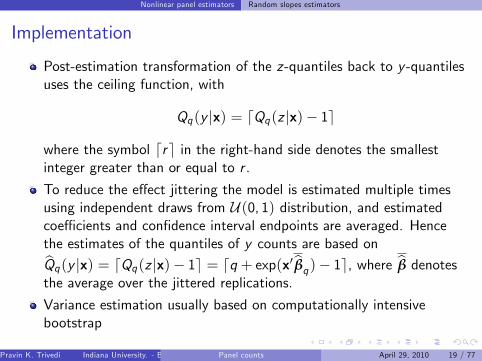
Post-estimation transformation of the z-quantiles back to y -quantilesuses the ceiling function, with
Qq(y jx) = dQq(z jx) 1e
where the symbol dre in the right-hand side denotes the smallestinteger greater than or equal to r .
To reduce the e¤ect jittering the model is estimated multiple timesusing independent draws from U (0, 1) distribution, and estimatedcoe¢ cients and condence interval endpoints are averaged. Hencethe estimates of the quantiles of y counts are based onbQq(y jx) = dQq(z jx) 1e = dq + exp(x0bβq) 1e, where bβ denotesthe average over the jittered replications.
Variance estimation usually based on computationally intensivebootstrap
Pravin K. Trivedi Indiana University. - Bloomington (Prepared for 2010 Mexican Stata Users Group meeting, based on A. Colin Cameron and Pravin K. Trivedi (2005), Microeconometrics: Methods and Applications (MMA), C.U.P. MMA, chapters 21-23 and A. Colin Cameron and Pravin K. Trivedi (2010), Microeconometrics using Stata Revised edition (MUSR), Stata Press. MUSR, chapters 8;18. )Panel counts April 29, 2010 19 / 77

Nonlinear panel estimators Random slopes estimators
QCR method of Machado and Santos Silva can be implemented usingStata add-on command qcount, due to Miranda (2006). Thecommand syntax is:
qcount depvar [indepvars ] [if ] [in], quantile(number) [, repetition(#)]
where quantile(number) species the quantile to be estimated andrepetition(#)species the number of jittered samples to be used tocalculate the parameters of the model, the default value being 1000.
Panel models can be estimated treating the data as repeated crosssections, as in PA approach.
Main attraction is the ability to study di¤erences in marginal e¤ectsat di¤erent quantiles.
The post-estimation command qcount_mfx computes marginale¤ects for the model, evaluated at the means of the regressors.
Pravin K. Trivedi Indiana University. - Bloomington (Prepared for 2010 Mexican Stata Users Group meeting, based on A. Colin Cameron and Pravin K. Trivedi (2005), Microeconometrics: Methods and Applications (MMA), C.U.P. MMA, chapters 21-23 and A. Colin Cameron and Pravin K. Trivedi (2010), Microeconometrics using Stata Revised edition (MUSR), Stata Press. MUSR, chapters 8;18. )Panel counts April 29, 2010 20 / 77

Nonlinear panel estimators Random slopes estimators
QCR Example - Winkelmann, JHE 2006Using an unbalanced sample (1995-1999) from GSOEP, Winkelmannanalyzes the di¤erential impact of healthcare reform on distribution ofdoctor visits across quantiles.
Pravin K. Trivedi Indiana University. - Bloomington (Prepared for 2010 Mexican Stata Users Group meeting, based on A. Colin Cameron and Pravin K. Trivedi (2005), Microeconometrics: Methods and Applications (MMA), C.U.P. MMA, chapters 21-23 and A. Colin Cameron and Pravin K. Trivedi (2010), Microeconometrics using Stata Revised edition (MUSR), Stata Press. MUSR, chapters 8;18. )Panel counts April 29, 2010 21 / 77

Nonlinear panel estimators Random slopes estimators
QR and panel data: pros and cons
Excess zeros can make identication of lower quantiles di¢ cult.
Can QR accommodate xed and random e¤ects?
Interpretation of xed e¤ects in QR context is somewhat tenuous; seeKoenker (2004).
QR has been extended to accommodate censoring, endogenousregressors; see Chernozhukov et al (2009)
QR has also been extended to handle lagged dependent variable.
Pravin K. Trivedi Indiana University. - Bloomington (Prepared for 2010 Mexican Stata Users Group meeting, based on A. Colin Cameron and Pravin K. Trivedi (2005), Microeconometrics: Methods and Applications (MMA), C.U.P. MMA, chapters 21-23 and A. Colin Cameron and Pravin K. Trivedi (2010), Microeconometrics using Stata Revised edition (MUSR), Stata Press. MUSR, chapters 8;18. )Panel counts April 29, 2010 22 / 77

Nonlinear panel estimators Random slopes estimators
11. Nonlinear random slopes estimators
Can extend to random slopes by adding an assumption about thedistribution of slopes.
I Nonlinear generalization of xtmixedI Then higher-dimensional numerical integral.I Use adaptive Gaussian quadrature
Stata commands are:I xtmelogit for binary dataI xtmepoisson for counts
Stata add-on that is very rich:I gllamm (generalized linear and latent mixed models); can be quiteslow!
I Developed by Sophia Rabe-Hesketh and Anders Skrondal.
Pravin K. Trivedi Indiana University. - Bloomington (Prepared for 2010 Mexican Stata Users Group meeting, based on A. Colin Cameron and Pravin K. Trivedi (2005), Microeconometrics: Methods and Applications (MMA), C.U.P. MMA, chapters 21-23 and A. Colin Cameron and Pravin K. Trivedi (2010), Microeconometrics using Stata Revised edition (MUSR), Stata Press. MUSR, chapters 8;18. )Panel counts April 29, 2010 23 / 77
Nonlinear panel estimators Fixed e¤ects estimators
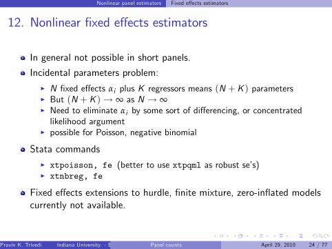
12. Nonlinear xed e¤ects estimators
In general not possible in short panels.
Incidental parameters problem:I N xed e¤ects αi plus K regressors means (N +K ) parametersI But (N +K )! ∞ as N ! ∞I Need to eliminate αi by some sort of di¤erencing, or concentratedlikelihood argument
I possible for Poisson, negative binomial
Stata commandsI xtpoisson, fe (better to use xtpqml as robust ses)I xtnbreg, fe
Fixed e¤ects extensions to hurdle, nite mixture, zero-inated modelscurrently not available.
Pravin K. Trivedi Indiana University. - Bloomington (Prepared for 2010 Mexican Stata Users Group meeting, based on A. Colin Cameron and Pravin K. Trivedi (2005), Microeconometrics: Methods and Applications (MMA), C.U.P. MMA, chapters 21-23 and A. Colin Cameron and Pravin K. Trivedi (2010), Microeconometrics using Stata Revised edition (MUSR), Stata Press. MUSR, chapters 8;18. )Panel counts April 29, 2010 24 / 77
Nonlinear panel estimators Fixed e¤ects estimators
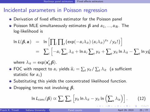
Incidental parameters in Poisson regressionDerivation of xed e¤ects estimator for the Poisson panel
Poisson MLE simultaneously estimates β and α1, ..., αN . Thelog-likelihood is
ln L(β, α) = lnh∏i ∏tfexp(αiλit ) (αiλit )
yit /yit !gi
= ∑i
hαi ∑t λit + ln αi ∑t yit +∑t yit lnλit ∑t ln yit !
i,(11)
where λit = exp(x0itβ).FOC with respect to αi yields bαi = ∑t yit/ ∑t λit (a su¢ cientstatistic for αi )
Substituting this yields the concentrated likelihood function.
Dropping terms not involving β,
ln Lconc(β) _ ∑i ∑t
hyit lnλit yit ln
∑s λis
i. (12)
Pravin K. Trivedi Indiana University. - Bloomington (Prepared for 2010 Mexican Stata Users Group meeting, based on A. Colin Cameron and Pravin K. Trivedi (2005), Microeconometrics: Methods and Applications (MMA), C.U.P. MMA, chapters 21-23 and A. Colin Cameron and Pravin K. Trivedi (2010), Microeconometrics using Stata Revised edition (MUSR), Stata Press. MUSR, chapters 8;18. )Panel counts April 29, 2010 25 / 77

Nonlinear panel estimators Fixed e¤ects estimators
Interpretation
Here is no incidental parameters problem.
Consistent estimates of β for xed T and N ! ∞ can be obtained bymaximization of ln Lconc(β)
FOC with respect to β yields rst-order conditions
∑i ∑t
hyitxit yit
h∑s λisxis
i/h∑s λis
ii= 0,
that can be re-expressed as
N
∑i=1
T
∑t=1xit
yit
λitλiyi
= 0, (13)
Pravin K. Trivedi Indiana University. - Bloomington (Prepared for 2010 Mexican Stata Users Group meeting, based on A. Colin Cameron and Pravin K. Trivedi (2005), Microeconometrics: Methods and Applications (MMA), C.U.P. MMA, chapters 21-23 and A. Colin Cameron and Pravin K. Trivedi (2010), Microeconometrics using Stata Revised edition (MUSR), Stata Press. MUSR, chapters 8;18. )Panel counts April 29, 2010 26 / 77
Nonlinear panel estimators Fixed e¤ects estimators
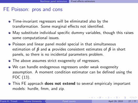
FE Poisson: pros and cons
Time-invariant regressors will be eliminated also by thetransformation. Some marginal e¤ects not identied.
May substitute individual specic dummy variables, though this raisessome computational issues.
Poisson and linear panel model special in that simultaneousestimation of β and α provides consistent estimates of β in shortpanels, so there is no incidental parameters problem.
The above assumes strict exogeneity of regressors.
We can handle endogenous regressors under weak exogeneityassumption. A moment condition estimator can be dened using theFOC (13).
This FE approach does not extend to several empiricaly importantmodels: hurdle, fmm, and zip.
Pravin K. Trivedi Indiana University. - Bloomington (Prepared for 2010 Mexican Stata Users Group meeting, based on A. Colin Cameron and Pravin K. Trivedi (2005), Microeconometrics: Methods and Applications (MMA), C.U.P. MMA, chapters 21-23 and A. Colin Cameron and Pravin K. Trivedi (2010), Microeconometrics using Stata Revised edition (MUSR), Stata Press. MUSR, chapters 8;18. )Panel counts April 29, 2010 27 / 77
Nonlinear panel estimators Fixed e¤ects estimators
Ad hoc methods for handling xed e¤ects
Are we making too much of the xed e¤ects and the associatedincidental paramnetr problem?
The dummy variables solution; Allison (2009); Greene (2004).
Pravin K. Trivedi Indiana University. - Bloomington (Prepared for 2010 Mexican Stata Users Group meeting, based on A. Colin Cameron and Pravin K. Trivedi (2005), Microeconometrics: Methods and Applications (MMA), C.U.P. MMA, chapters 21-23 and A. Colin Cameron and Pravin K. Trivedi (2010), Microeconometrics using Stata Revised edition (MUSR), Stata Press. MUSR, chapters 8;18. )Panel counts April 29, 2010 28 / 77

Computation with Stata Commands
13. Stata CommandsNonlinear panel estimators
Estimator Count dataPooled poisson; nbregQuantile qcount q(%), rep(#)
FMMfmm components(#) mixtureof(poisson)fmm components(#) mixtureof(nbreg)
GEE (PA) xtgee,family(poisson)xtgee,family(nbinomial)
RE xtpoisson, rextnbreg, fe
Random slopes xtmepoissonFE xtpoisson, fe
xtnbreg, fe
FMM is not part of o¢ cial Stata but is in the public domain and canbe added
Pravin K. Trivedi Indiana University. - Bloomington (Prepared for 2010 Mexican Stata Users Group meeting, based on A. Colin Cameron and Pravin K. Trivedi (2005), Microeconometrics: Methods and Applications (MMA), C.U.P. MMA, chapters 21-23 and A. Colin Cameron and Pravin K. Trivedi (2010), Microeconometrics using Stata Revised edition (MUSR), Stata Press. MUSR, chapters 8;18. )Panel counts April 29, 2010 29 / 77

Computation with Stata Commands Data example
Panel counts: data example
Data from Rand health insurance experiment.I y is number of doctor visits.
year float %9.0g study yearid float %9.0g person id, leading digit is sitchild float %9.0g childlfam float %9.0g log of family sizeage float %9.0g age that yearfemale float %9.0g femalendisease float %9.0g count of chronic diseases balcoins float %9.0g log(coinsurance+1)mdu float %9.0g number facetofact md visits
variable name type format label variable labelstorage display value
. describe mdu lcoins ndisease female age lfam child id year
. use mus18data.dta, clear
Pravin K. Trivedi Indiana University. - Bloomington (Prepared for 2010 Mexican Stata Users Group meeting, based on A. Colin Cameron and Pravin K. Trivedi (2005), Microeconometrics: Methods and Applications (MMA), C.U.P. MMA, chapters 21-23 and A. Colin Cameron and Pravin K. Trivedi (2010), Microeconometrics using Stata Revised edition (MUSR), Stata Press. MUSR, chapters 8;18. )Panel counts April 29, 2010 30 / 77

Computation with Stata Commands Data example
Dependent variable mdu is very overdispersed: bV[y ] = 4.502 ' 7 y .
year 20186 2.420044 1.217237 1 5id 20186 357971.2 180885.6 125024 632167
child 20186 .4014168 .4901972 0 1 lfam 20186 1.248404 .5390681 0 2.639057
age 20186 25.71844 16.76759 0 64.27515female 20186 .5169424 .4997252 0 1
ndisease 20186 11.2445 6.741647 0 58.6lcoins 20186 2.383588 2.041713 0 4.564348
mdu 20186 2.860696 4.504765 0 77
Variable Obs Mean Std. Dev. Min Max
. summarize mdu lcoins ndisease female age lfam child id year
Pravin K. Trivedi Indiana University. - Bloomington (Prepared for 2010 Mexican Stata Users Group meeting, based on A. Colin Cameron and Pravin K. Trivedi (2005), Microeconometrics: Methods and Applications (MMA), C.U.P. MMA, chapters 21-23 and A. Colin Cameron and Pravin K. Trivedi (2010), Microeconometrics using Stata Revised edition (MUSR), Stata Press. MUSR, chapters 8;18. )Panel counts April 29, 2010 31 / 77

Computation with Stata Commands Data example
Panel is unbalanced. Most are in for 3 years or 5 years.
1 2 3 3 5 5 5Distribution of T_i: min 5% 25% 50% 75% 95% max
(id*year uniquely identifies each observation)Span(year) = 5 periodsDelta(year) = 1 unit
year: 1, 2, ..., 5 T = 5id: 125024, 125025, ..., 632167 n = 5908
. xtdescribe
Pravin K. Trivedi Indiana University. - Bloomington (Prepared for 2010 Mexican Stata Users Group meeting, based on A. Colin Cameron and Pravin K. Trivedi (2005), Microeconometrics: Methods and Applications (MMA), C.U.P. MMA, chapters 21-23 and A. Colin Cameron and Pravin K. Trivedi (2010), Microeconometrics using Stata Revised edition (MUSR), Stata Press. MUSR, chapters 8;18. )Panel counts April 29, 2010 32 / 77
Computation with Stata Commands Data example
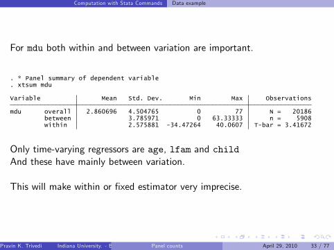
For mdu both within and between variation are important.
within 2.575881 34.47264 40.0607 Tbar = 3.41672 between 3.785971 0 63.33333 n = 5908mdu overall 2.860696 4.504765 0 77 N = 20186
Variable Mean Std. Dev. Min Max Observations
. xtsum mdu
. * Panel summary of dependent variable
Only time-varying regressors are age, lfam and childAnd these have mainly between variation.
This will make within or xed estimator very imprecise.
Pravin K. Trivedi Indiana University. - Bloomington (Prepared for 2010 Mexican Stata Users Group meeting, based on A. Colin Cameron and Pravin K. Trivedi (2005), Microeconometrics: Methods and Applications (MMA), C.U.P. MMA, chapters 21-23 and A. Colin Cameron and Pravin K. Trivedi (2010), Microeconometrics using Stata Revised edition (MUSR), Stata Press. MUSR, chapters 8;18. )Panel counts April 29, 2010 33 / 77

Likelihood-based Panel Count Estimators
14. Panel Poisson
Consider four panel Poisson estimatorsI Pooled Poisson with cluster-robust errorsI Population-averaged Poisson (GEE)I Poisson random e¤ects (gamma and normal)I Poisson xed e¤ects
Can additionally apply most of these to negative binomial.
And can extend FE to dynamic panel Poisson where yi ,t1 is aregressor.
Pravin K. Trivedi Indiana University. - Bloomington (Prepared for 2010 Mexican Stata Users Group meeting, based on A. Colin Cameron and Pravin K. Trivedi (2005), Microeconometrics: Methods and Applications (MMA), C.U.P. MMA, chapters 21-23 and A. Colin Cameron and Pravin K. Trivedi (2010), Microeconometrics using Stata Revised edition (MUSR), Stata Press. MUSR, chapters 8;18. )Panel counts April 29, 2010 34 / 77

Likelihood-based Panel Count Estimators MLE Estimation
Model Moment spec. Estimating equations
Pooled E[y it jx it ] = exp (x0itβ) ∑N
i=1 ∑Tt=1 xit (yit µit ) = 0
Poisson where µit = exp(x0itβ)
PA ρts = Cor[(yit exp(x 0itβ))(yis exp(x 0isβ))].
RE E[y it jαi , x it ] ∑Ni=1 ∑T
t=1 xit
yit µit
yi + η/Tµi + η/T
= 0
Poisson = αi exp (x0itβ) µi = T
1 ∑t exp(x0itβ); η = var(αi )
FE Pois E[y it jαi , x it ] = αi exp (x0itβ) ∑N
i=1 ∑Tt=1 xit
yit µit
yiµi
= 0,
Pravin K. Trivedi Indiana University. - Bloomington (Prepared for 2010 Mexican Stata Users Group meeting, based on A. Colin Cameron and Pravin K. Trivedi (2005), Microeconometrics: Methods and Applications (MMA), C.U.P. MMA, chapters 21-23 and A. Colin Cameron and Pravin K. Trivedi (2010), Microeconometrics using Stata Revised edition (MUSR), Stata Press. MUSR, chapters 8;18. )Panel counts April 29, 2010 35 / 77
Likelihood-based Panel Count Estimators Pooled Poisson
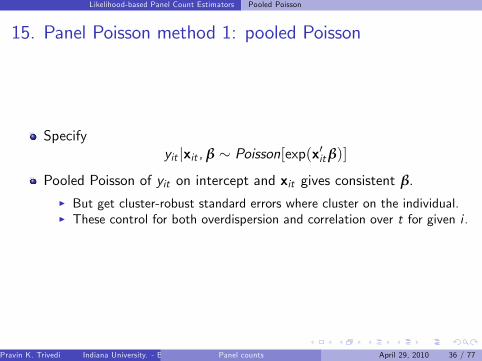
15. Panel Poisson method 1: pooled Poisson
Specifyyit jxit , β Poisson[exp(x0itβ)]
Pooled Poisson of yit on intercept and xit gives consistent β.I But get cluster-robust standard errors where cluster on the individual.I These control for both overdispersion and correlation over t for given i .
Pravin K. Trivedi Indiana University. - Bloomington (Prepared for 2010 Mexican Stata Users Group meeting, based on A. Colin Cameron and Pravin K. Trivedi (2005), Microeconometrics: Methods and Applications (MMA), C.U.P. MMA, chapters 21-23 and A. Colin Cameron and Pravin K. Trivedi (2010), Microeconometrics using Stata Revised edition (MUSR), Stata Press. MUSR, chapters 8;18. )Panel counts April 29, 2010 36 / 77

Likelihood-based Panel Count Estimators Pooled Poisson
Pooled Poisson with cluster-robust standard errors
_cons .748789 .0785738 9.53 0.000 .5947872 .9027907 child .1030453 .0506901 2.03 0.042 .0036944 .2023961 lfam .1481981 .0323434 4.58 0.000 .21159 .0848062 age .0040585 .0016891 2.40 0.016 .000748 .0073691 female .1717862 .0342551 5.01 0.000 .1046473 .2389251 ndisease .0339334 .0026024 13.04 0.000 .0288328 .039034 lcoins .0808023 .0080013 10.10 0.000 .0964846 .0651199
mdu Coef. Std. Err. z P>|z| [95% Conf. Interval] Robust
(Std. Err. adjusted for 5908 clusters in id)
Log pseudolikelihood = 62579.401 Pseudo R2 = 0.0609 Prob > chi2 = 0.0000 Wald chi2(6) = 476.93Poisson regression Number of obs = 20186
Iteration 2: log pseudolikelihood = 62579.401Iteration 1: log pseudolikelihood = 62579.401Iteration 0: log pseudolikelihood = 62580.248
. poisson mdu lcoins ndisease female age lfam child, vce(cluster id)
. * Pooled Poisson estimator with clusterrobust standard errors
By comparison, the default (non cluster-robust) s.e.s are 1/4 as large.) The default (non cluster-robust) t-statistics are 4 times as large!!
Pravin K. Trivedi Indiana University. - Bloomington (Prepared for 2010 Mexican Stata Users Group meeting, based on A. Colin Cameron and Pravin K. Trivedi (2005), Microeconometrics: Methods and Applications (MMA), C.U.P. MMA, chapters 21-23 and A. Colin Cameron and Pravin K. Trivedi (2010), Microeconometrics using Stata Revised edition (MUSR), Stata Press. MUSR, chapters 8;18. )Panel counts April 29, 2010 37 / 77

Likelihood-based Panel Count Estimators Population-averaged Poisson (PA or GEE)
16. Panel Poisson method 2: population-averaged
Assume that for the i th observation moments are like for GLM Poisson
E[yit jxit ] = exp(x0itβ)V[yit jxit ] = φ exp(x0itβ).
Stack the conditional means for the i th individual:
E[yi jXi ] = mi (β) =
264 exp(x0i1β)...
exp(x0iT β)
375 .where yi = [yi1, ..., yiT ]0 and Xi = [xi1, ..., xiT ]0.Stack the conditional variances for the i th individual.
I With no correlation
V[yi jXi ] = φHi (β) = φDiag[exp(x0itβ)].
Pravin K. Trivedi Indiana University. - Bloomington (Prepared for 2010 Mexican Stata Users Group meeting, based on A. Colin Cameron and Pravin K. Trivedi (2005), Microeconometrics: Methods and Applications (MMA), C.U.P. MMA, chapters 21-23 and A. Colin Cameron and Pravin K. Trivedi (2010), Microeconometrics using Stata Revised edition (MUSR), Stata Press. MUSR, chapters 8;18. )Panel counts April 29, 2010 38 / 77
Likelihood-based Panel Count Estimators Population-averaged Poisson (PA or GEE)
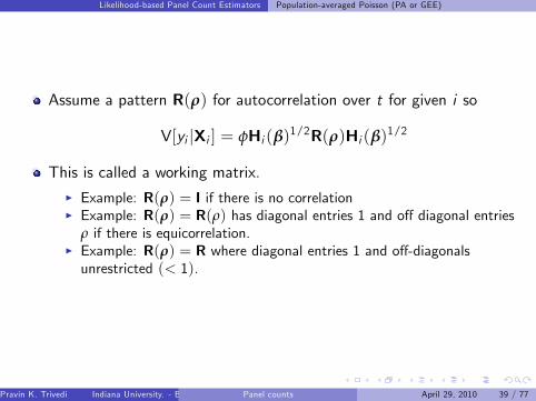
Assume a pattern R(ρ) for autocorrelation over t for given i so
V[yi jXi ] = φHi (β)1/2R(ρ)Hi (β)1/2
This is called a working matrix.I Example: R(ρ) = I if there is no correlationI Example: R(ρ) = R(ρ) has diagonal entries 1 and o¤ diagonal entries
ρ if there is equicorrelation.I Example: R(ρ) = R where diagonal entries 1 and o¤-diagonalsunrestricted (< 1).
Pravin K. Trivedi Indiana University. - Bloomington (Prepared for 2010 Mexican Stata Users Group meeting, based on A. Colin Cameron and Pravin K. Trivedi (2005), Microeconometrics: Methods and Applications (MMA), C.U.P. MMA, chapters 21-23 and A. Colin Cameron and Pravin K. Trivedi (2010), Microeconometrics using Stata Revised edition (MUSR), Stata Press. MUSR, chapters 8;18. )Panel counts April 29, 2010 39 / 77
Likelihood-based Panel Count Estimators GLM Estimation
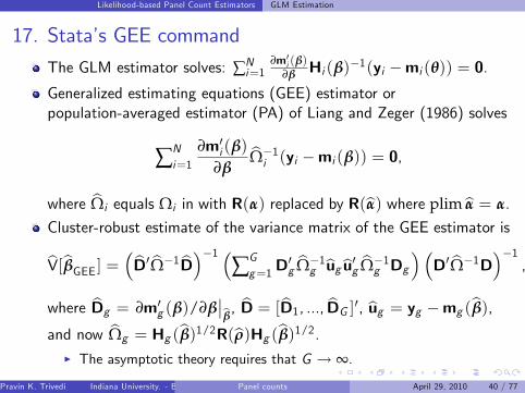
17. Statas GEE command
The GLM estimator solves: ∑Ni=1
∂m0i (β)∂β Hi (β)1(yi mi (θ)) = 0.
Generalized estimating equations (GEE) estimator orpopulation-averaged estimator (PA) of Liang and Zeger (1986) solves
∑Ni=1
∂m0i (β)∂β
bΩ1i (yi mi (β)) = 0,
where bΩi equals Ωi in with R(α) replaced by R(bα) where plim bα = α.
Cluster-robust estimate of the variance matrix of the GEE estimator is
bV[bβGEE ] = bD0 bΩ1 bD1 ∑Gg=1D
0gbΩ1g bugbu0g bΩ1
g Dg D0 bΩ1D
1,
where bDg = ∂m0g (β)/∂βbβ, bD = [bD1, ..., bDG ]0, bug = yg mg (bβ),
and now bΩg = Hg (bβ)1/2R(bρ)Hg (bβ)1/2.I The asymptotic theory requires that G ! ∞.
Pravin K. Trivedi Indiana University. - Bloomington (Prepared for 2010 Mexican Stata Users Group meeting, based on A. Colin Cameron and Pravin K. Trivedi (2005), Microeconometrics: Methods and Applications (MMA), C.U.P. MMA, chapters 21-23 and A. Colin Cameron and Pravin K. Trivedi (2010), Microeconometrics using Stata Revised edition (MUSR), Stata Press. MUSR, chapters 8;18. )Panel counts April 29, 2010 40 / 77
Likelihood-based Panel Count Estimators GLM Estimation
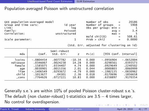
Population-averaged Poisson with unstructured correlation
_cons .7764626 .0717221 10.83 0.000 .6358897 .9170354 child .1013677 .04301 2.36 0.018 .0170696 .1856658 lfam .1406549 .0293672 4.79 0.000 .1982135 .0830962 age .0030901 .0015356 2.01 0.044 .0000803 .0060999 female .1585075 .0334407 4.74 0.000 .0929649 .2240502 ndisease .0346067 .0024238 14.28 0.000 .0298561 .0393573 lcoins .0804454 .0077782 10.34 0.000 .0956904 .0652004
mdu Coef. Std. Err. z P>|z| [95% Conf. Interval] Semirobust
(Std. Err. adjusted for clustering on id)
Scale parameter: 1 Prob > chi2 = 0.0000Wald chi2(6) = 508.61
Correlation: unstructured max = 5Family: Poisson avg = 3.4Link: log Obs per group: min = 1Group and time vars: id year Number of groups = 5908GEE populationaveraged model Number of obs = 20186
Generally s.e.s are within 10% of pooled Poisson cluster-robust s.e.s.The default (non cluster-robust) t-statistics are 3.5 4 times larger,No control for overdispersion.
Pravin K. Trivedi Indiana University. - Bloomington (Prepared for 2010 Mexican Stata Users Group meeting, based on A. Colin Cameron and Pravin K. Trivedi (2005), Microeconometrics: Methods and Applications (MMA), C.U.P. MMA, chapters 21-23 and A. Colin Cameron and Pravin K. Trivedi (2010), Microeconometrics using Stata Revised edition (MUSR), Stata Press. MUSR, chapters 8;18. )Panel counts April 29, 2010 41 / 77
Likelihood-based Panel Count Estimators GLM Estimation
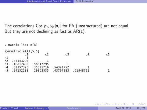
The correlations Cor[yit , yis jxi ] for PA (unstructured) are not equal.But they are not declining as fast as AR(1).
r5 .34152288 .29803555 .43767583 .61948751 1r4 .32357326 .35321716 .54321752 1r3 .40817495 .58547795 1r2 .53143297 1r1 1 c1 c2 c3 c4 c5symmetric e(R)[5,5]
. matrix list e(R)
Pravin K. Trivedi Indiana University. - Bloomington (Prepared for 2010 Mexican Stata Users Group meeting, based on A. Colin Cameron and Pravin K. Trivedi (2005), Microeconometrics: Methods and Applications (MMA), C.U.P. MMA, chapters 21-23 and A. Colin Cameron and Pravin K. Trivedi (2010), Microeconometrics using Stata Revised edition (MUSR), Stata Press. MUSR, chapters 8;18. )Panel counts April 29, 2010 42 / 77
Likelihood-based Panel Count Estimators Poisson random e¤ects
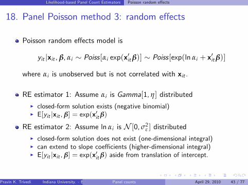
18. Panel Poisson method 3: random e¤ects
Poisson random e¤ects model is
yit jxit , β, αi Poiss [αi exp(x0itβ)] Poiss [exp(ln αi + x0itβ)]
where αi is unobserved but is not correlated with xit .
RE estimator 1: Assume αi is Gamma[1, η] distributedI closed-form solution exists (negative binomial)I E[yit jxit , β] = exp(x0itβ)
RE estimator 2: Assume ln αi is N [0, σ2ε ] distributedI closed-form solution does not exist (one-dimensional integral)I can extend to slope coe¢ cients (higher-dimensional integral)I E[yit jxit , β] = exp(x0itβ) aside from translation of intercept.
Pravin K. Trivedi Indiana University. - Bloomington (Prepared for 2010 Mexican Stata Users Group meeting, based on A. Colin Cameron and Pravin K. Trivedi (2005), Microeconometrics: Methods and Applications (MMA), C.U.P. MMA, chapters 21-23 and A. Colin Cameron and Pravin K. Trivedi (2010), Microeconometrics using Stata Revised edition (MUSR), Stata Press. MUSR, chapters 8;18. )Panel counts April 29, 2010 43 / 77
Likelihood-based Panel Count Estimators Poisson random e¤ects
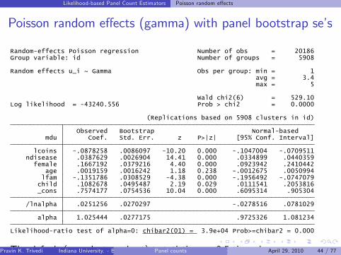
Poisson random e¤ects (gamma) with panel bootstrap ses
Likelihoodratio test of alpha=0: chibar2(01) = 3.9e+04 Prob>=chibar2 = 0.000
alpha 1.025444 .0277175 .9725326 1.081234
/lnalpha .0251256 .0270297 .0278516 .0781029
_cons .7574177 .0754536 10.04 0.000 .6095314 .905304 child .1082678 .0495487 2.19 0.029 .0111541 .2053816 lfam .1351786 .0308529 4.38 0.000 .1956492 .0747079 age .0019159 .0016242 1.18 0.238 .0012675 .0050994 female .1667192 .0379216 4.40 0.000 .0923942 .2410442 ndisease .0387629 .0026904 14.41 0.000 .0334899 .0440359 lcoins .0878258 .0086097 10.20 0.000 .1047004 .0709511
mdu Coef. Std. Err. z P>|z| [95% Conf. Interval] Observed Bootstrap Normalbased
(Replications based on 5908 clusters in id)
Log likelihood = 43240.556 Prob > chi2 = 0.0000 Wald chi2(6) = 529.10
max = 5 avg = 3.4Random effects u_i ~ Gamma Obs per group: min = 1
Group variable: id Number of groups = 5908Randomeffects Poisson regression Number of obs = 20186
The default (non cluster-robust) t-statistics are 2.5 times largerbecause default do not control for overdispersion.
Pravin K. Trivedi Indiana University. - Bloomington (Prepared for 2010 Mexican Stata Users Group meeting, based on A. Colin Cameron and Pravin K. Trivedi (2005), Microeconometrics: Methods and Applications (MMA), C.U.P. MMA, chapters 21-23 and A. Colin Cameron and Pravin K. Trivedi (2010), Microeconometrics using Stata Revised edition (MUSR), Stata Press. MUSR, chapters 8;18. )Panel counts April 29, 2010 44 / 77

Likelihood-based Panel Count Estimators Poisson random e¤ects
19. Poisson xed e¤ects with panel bootstrap ses
child .1059867 .0738452 1.44 0.151 .0387472 .2507206 lfam .0877134 .1125783 0.78 0.436 .132936 .3083627 age .0112009 .0095077 1.18 0.239 .0298356 .0074339
mdu Coef. Std. Err. z P>|z| [95% Conf. Interval] Observed Bootstrap Normalbased
(Replications based on 4977 clusters in id)
Log likelihood = 24173.211 Prob > chi2 = 0.2002 Wald chi2(3) = 4.64
max = 5 avg = 3.6 Obs per group: min = 2
Group variable: id Number of groups = 4977Conditional fixedeffects Poisson regression Number of obs = 17791
.................................................. 100
.................................................. 50 1 2 3 4 5
Bootstrap replications (100)
(running xtpoisson on estimation sample). xtpoisson mdu lcoins ndisease female age lfam child, fe vce(boot, reps(100) seed(10101))
The default (non cluster-robust) t-statistics are 2 times larger.Pravin K. Trivedi Indiana University. - Bloomington (Prepared for 2010 Mexican Stata Users Group meeting, based on A. Colin Cameron and Pravin K. Trivedi (2005), Microeconometrics: Methods and Applications (MMA), C.U.P. MMA, chapters 21-23 and A. Colin Cameron and Pravin K. Trivedi (2010), Microeconometrics using Stata Revised edition (MUSR), Stata Press. MUSR, chapters 8;18. )Panel counts April 29, 2010 45 / 77
Likelihood-based Panel Count Estimators Poisson random e¤ects
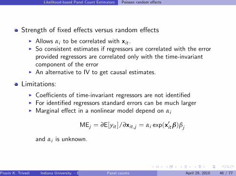
Strength of xed e¤ects versus random e¤ectsI Allows αi to be correlated with xit .I So consistent estimates if regressors are correlated with the errorprovided regressors are correlated only with the time-invariantcomponent of the error
I An alternative to IV to get causal estimates.
Limitations:I Coe¢ cients of time-invariant regressors are not identiedI For identied regressors standard errors can be much largerI Marginal e¤ect in a nonlinear model depend on αi
MEj = ∂E[yit ]/∂xit ,j = αi exp(x0itβ)βj
and αi is unknown.
Pravin K. Trivedi Indiana University. - Bloomington (Prepared for 2010 Mexican Stata Users Group meeting, based on A. Colin Cameron and Pravin K. Trivedi (2005), Microeconometrics: Methods and Applications (MMA), C.U.P. MMA, chapters 21-23 and A. Colin Cameron and Pravin K. Trivedi (2010), Microeconometrics using Stata Revised edition (MUSR), Stata Press. MUSR, chapters 8;18. )Panel counts April 29, 2010 46 / 77
Likelihood-based Panel Count Estimators Poisson random e¤ects
Panel Poisson: estimator comparison
Compare following estimatorsI pooled Poisson with cluster-robust s.e.sI pooled population averaged Poisson with unstructured correlations andcluster-robust s.e.s
I random e¤ects Poisson with gamma random e¤ect and cluster-robusts.e.s
I random e¤ects Poisson with normal random e¤ect and default s.e.sI xed e¤ects Poisson and cluster-robust s.e.s
Find thatI similar results for all RE modelsI note that these data are not good to illustrate FE as regressors havelittle within variation.
Pravin K. Trivedi Indiana University. - Bloomington (Prepared for 2010 Mexican Stata Users Group meeting, based on A. Colin Cameron and Pravin K. Trivedi (2005), Microeconometrics: Methods and Applications (MMA), C.U.P. MMA, chapters 21-23 and A. Colin Cameron and Pravin K. Trivedi (2010), Microeconometrics using Stata Revised edition (MUSR), Stata Press. MUSR, chapters 8;18. )Panel counts April 29, 2010 47 / 77
Likelihood-based Panel Count Estimators Poisson random e¤ects
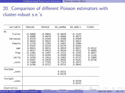
20. Comparison of di¤erent Poisson estimators withcluster-robust s.e.s
legend: b/se
ll 62579 43241 43227 24173 N 20186 20186 20186 20186 17791Statistics
0.0255 _cons 0.0550lnsig2u
0.0270 _cons 0.0251lnalpha
0.0786 0.0717 0.0755 0.0642 _cons 0.7488 0.7765 0.7574 0.2873
0.0507 0.0430 0.0495 0.0345 0.0738 child 0.1030 0.1014 0.1083 0.0737 0.1060
0.0323 0.0294 0.0309 0.0265 0.1126 lfam 0.1482 0.1407 0.1352 0.1443 0.0877
0.0017 0.0015 0.0016 0.0012 0.0095 age 0.0041 0.0031 0.0019 0.0027 0.0112
0.0343 0.0334 0.0379 0.0305 female 0.1718 0.1585 0.1667 0.2084
0.0026 0.0024 0.0027 0.0023 ndisease 0.0339 0.0346 0.0388 0.0409
0.0080 0.0078 0.0086 0.0073 lcoins 0.0808 0.0804 0.0878 0.1145#1
Variable POOLED POPAVE RE_GAMMA RE_NOR~L FIXED
Pravin K. Trivedi Indiana University. - Bloomington (Prepared for 2010 Mexican Stata Users Group meeting, based on A. Colin Cameron and Pravin K. Trivedi (2005), Microeconometrics: Methods and Applications (MMA), C.U.P. MMA, chapters 21-23 and A. Colin Cameron and Pravin K. Trivedi (2010), Microeconometrics using Stata Revised edition (MUSR), Stata Press. MUSR, chapters 8;18. )Panel counts April 29, 2010 48 / 77

Likelihood-based Panel Count Estimators Moment based estimation of FE count panels
Predetrmined means regressor correlated with current and pastshoocks but not future shocks: E [uitxis ] = 0 for s t, but 6= 0 forS < t.
Two specications are considered:
yit = exp(x0itβ)νiwityit = exp(x0itβ)νi + wit
A quasi-di¤erencing transformation is used to eliminate the xede¤ect.
Then a moment condition is constructed for estimation.
Depending upon which specication is used di¤erent momentconditions obtain.
Chamberlain and Wooldridge derive quasi-di¤erencing transformationsthat are shown in the table below.
Pravin K. Trivedi Indiana University. - Bloomington (Prepared for 2010 Mexican Stata Users Group meeting, based on A. Colin Cameron and Pravin K. Trivedi (2005), Microeconometrics: Methods and Applications (MMA), C.U.P. MMA, chapters 21-23 and A. Colin Cameron and Pravin K. Trivedi (2010), Microeconometrics using Stata Revised edition (MUSR), Stata Press. MUSR, chapters 8;18. )Panel counts April 29, 2010 49 / 77
Likelihood-based Panel Count Estimators Moment based estimation of FE count panels
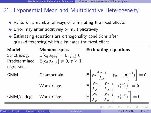
21. Exponential Mean and Multiplicative Heterogeneity
Relies on a number of ways of eliminating the xed e¤ects
Error may enter additively or multiplicatively
Estimating equations are orthogonality conditions afterquasi-di¤erencing which eliminates the xed e¤ect
Model Moment spec. Estimating equationsStrict exog. E[xituit+j ] = 0, j 0Predetermined E[xituits ] 6= 0, s 1regressors
GMM Chamberlain Eyit
λit1λit
yit1 jxt1i )
= 0
Wooldridge Eyitλit yit1
λit1jxt1i )
= 0
GMM/endog Wooldridge Eyitλit yit1
λit1jxt2i )
= 0
Pravin K. Trivedi Indiana University. - Bloomington (Prepared for 2010 Mexican Stata Users Group meeting, based on A. Colin Cameron and Pravin K. Trivedi (2005), Microeconometrics: Methods and Applications (MMA), C.U.P. MMA, chapters 21-23 and A. Colin Cameron and Pravin K. Trivedi (2010), Microeconometrics using Stata Revised edition (MUSR), Stata Press. MUSR, chapters 8;18. )Panel counts April 29, 2010 49 / 77

Likelihood-based Panel Count Estimators Computational Strategies for GMM
1 Use an interactive version of an estimation command (e.g. gmm);enter the function directly on the command line or dialog box byusing a substitutable expression.
2 Use a function evaluator program which gives more exibility indening your objective function; usually more complicated to use butmay be needed for more complicated problems.
Hint: In Stata a good place to start is the nl (nonlinear least squares)command. Then go on to gmm.
Most of the examples here involve substitutable expressions.Examples of function evaluator programs are in MUS and especially inStata manuals.
Example: ∑Ni=1 ∑T
t=1 xit
yit µit
yiµi
= 0,
Pravin K. Trivedi Indiana University. - Bloomington (Prepared for 2010 Mexican Stata Users Group meeting, based on A. Colin Cameron and Pravin K. Trivedi (2005), Microeconometrics: Methods and Applications (MMA), C.U.P. MMA, chapters 21-23 and A. Colin Cameron and Pravin K. Trivedi (2010), Microeconometrics using Stata Revised edition (MUSR), Stata Press. MUSR, chapters 8;18. )Panel counts April 29, 2010 50 / 77
Likelihood-based Panel Count Estimators Applications
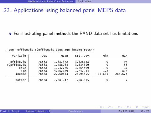
22. Applications using balanced panel MEPS data
For illustrating panel methods the RAND data set has limitations
totchr 78888 .7881047 1.081315 0 7
income 78888 27.60833 28.94855 63.631 264.674 age 78888 4.562129 1.742034 1.8 8.5 educ 78888 12.32776 3.264869 0 17 T0officevis 78888 1.488084 3.334559 0 58 officevis 78888 1.387372 3.328148 0 94
Variable Obs Mean Std. Dev. Min Max
. sum officevis T0officevis educ age income totchr
Pravin K. Trivedi Indiana University. - Bloomington (Prepared for 2010 Mexican Stata Users Group meeting, based on A. Colin Cameron and Pravin K. Trivedi (2005), Microeconometrics: Methods and Applications (MMA), C.U.P. MMA, chapters 21-23 and A. Colin Cameron and Pravin K. Trivedi (2010), Microeconometrics using Stata Revised edition (MUSR), Stata Press. MUSR, chapters 8;18. )Panel counts April 29, 2010 51 / 77

Likelihood-based Panel Count Estimators Applications
MEPS Data
Quarterly data for 2005-06
9861 100.00 XXXXXXXX
9861 100.00 100.00 11111111
Freq. Percent Cum. Pattern
8 8 8 8 8 8 8Distribution of T_i: min 5% 25% 50% 75% 95% max
(dupersid*timeindex uniquely identifies each observation)Span(timeindex) = 8 periodsDelta(timeindex) = 1 unit
timeindex: 1, 2, ..., 8 T = 8dupersid: 30002019, 30004010, ..., 38505016 n = 9861
. xtdes
Pravin K. Trivedi Indiana University. - Bloomington (Prepared for 2010 Mexican Stata Users Group meeting, based on A. Colin Cameron and Pravin K. Trivedi (2005), Microeconometrics: Methods and Applications (MMA), C.U.P. MMA, chapters 21-23 and A. Colin Cameron and Pravin K. Trivedi (2010), Microeconometrics using Stata Revised edition (MUSR), Stata Press. MUSR, chapters 8;18. )Panel counts April 29, 2010 52 / 77
Likelihood-based Panel Count Estimators Applications
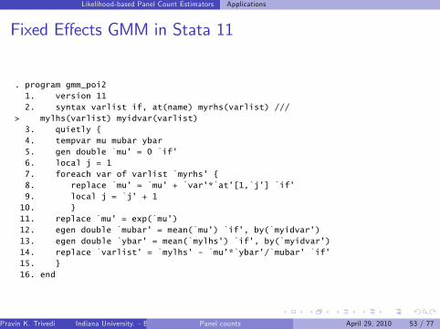
Fixed E¤ects GMM in Stata 11
16. end
15.
14. replace `varlist' = `mylhs' `mu'*`ybar'/`mubar' `if'
13. egen double `ybar' = mean(`mylhs') `if', by(`myidvar')
12. egen double `mubar' = mean(`mu') `if', by(`myidvar')
11. replace `mu' = exp(`mu')
10.
9. local j = `j' + 1
8. replace `mu' = `mu' + `var'*`at'[1,`j'] `if'
7. foreach var of varlist `myrhs'
6. local j = 1
5. gen double `mu' = 0 `if'
4. tempvar mu mubar ybar
3. quietly
> mylhs(varlist) myidvar(varlist)
2. syntax varlist if, at(name) myrhs(varlist) ///
1. version 11
. program gmm_poi2
Pravin K. Trivedi Indiana University. - Bloomington (Prepared for 2010 Mexican Stata Users Group meeting, based on A. Colin Cameron and Pravin K. Trivedi (2005), Microeconometrics: Methods and Applications (MMA), C.U.P. MMA, chapters 21-23 and A. Colin Cameron and Pravin K. Trivedi (2010), Microeconometrics using Stata Revised edition (MUSR), Stata Press. MUSR, chapters 8;18. )Panel counts April 29, 2010 53 / 77

Likelihood-based Panel Count Estimators Applications
Implementing xed e¤ects GMM in Stata 11
. estimates store PFEGMM
Instruments for equation 1: insprv age income totchr
/totchr .2211125 .3354182 0.66 0.510 .4362951 .8785201 /income .001128 .0013911 0.81 0.417 .0015984 .0038545 /age .5125841 13.1682 0.04 0.969 26.32178 25.29662 /insprv .0080549 .5460749 0.01 0.988 1.078342 1.062232
Coef. Std. Err. z P>|z| [95% Conf. Interval] Robust
Initial weight matrix: Unadjusted Number of obs = 78888Number of moments = 4Number of parameters = 4
GMM estimation
Iteration 3: GMM criterion Q(b) = 1.843e28Iteration 2: GMM criterion Q(b) = 1.583e14Iteration 1: GMM criterion Q(b) = 1.487e07Iteration 0: GMM criterion Q(b) = .00140916Step 1
> instruments(insprv age income totchr, noconstant) onestep> myidvar(dupersid) nequations(1) parameters(insprv age income totchr) ///. gmm gmm_poi2, mylhs(officevis) myrhs(insprv age income totchr) ///
Pravin K. Trivedi Indiana University. - Bloomington (Prepared for 2010 Mexican Stata Users Group meeting, based on A. Colin Cameron and Pravin K. Trivedi (2005), Microeconometrics: Methods and Applications (MMA), C.U.P. MMA, chapters 21-23 and A. Colin Cameron and Pravin K. Trivedi (2010), Microeconometrics using Stata Revised edition (MUSR), Stata Press. MUSR, chapters 8;18. )Panel counts April 29, 2010 54 / 77

Likelihood-based Panel Count Estimators Applications
Standard xed e¤ects panel Poisson
. estimates store PFE
totchr .2211125 .0091051 24.28 0.000 .2032669 .2389582 income .001128 .000258 4.37 0.000 .0006224 .0016336 age .5125841 .0629145 8.15 0.000 .6358943 .3892739 insprv .0080549 .027985 0.29 0.773 .0629046 .0467947
officevis Coef. Std. Err. z P>|z| [95% Conf. Interval]
Log likelihood = 84154.647 Prob > chi2 = 0.0000 Wald chi2(4) = 618.20
max = 8 avg = 8.0 Obs per group: min = 8
Group variable: dupersid Number of groups = 7961Conditional fixedeffects Poisson regression Number of obs = 63688
Iteration 3: log likelihood = 84154.647Iteration 2: log likelihood = 84154.647Iteration 1: log likelihood = 84154.68Iteration 0: log likelihood = 84468.435
note: 1900 groups (15200 obs) dropped because of all zero outcomes. xtpoisson officevis insprv age income totchr, fe. * Usual panel Poisson FE
No di¤erence in point estimates because MLE and GMM solve the sameFOC.
Pravin K. Trivedi Indiana University. - Bloomington (Prepared for 2010 Mexican Stata Users Group meeting, based on A. Colin Cameron and Pravin K. Trivedi (2005), Microeconometrics: Methods and Applications (MMA), C.U.P. MMA, chapters 21-23 and A. Colin Cameron and Pravin K. Trivedi (2010), Microeconometrics using Stata Revised edition (MUSR), Stata Press. MUSR, chapters 8;18. )Panel counts April 29, 2010 55 / 77
Likelihood-based Panel Count Estimators Applications
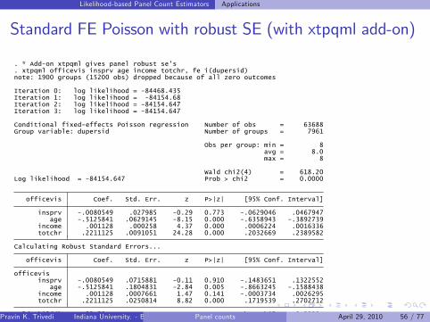
Standard FE Poisson with robust SE (with xtpqml add-on)
. estimates store PFECLU
Wald chi2(4) = 80.59 Prob > chi2 = 0.0000
totchr .2211125 .0250814 8.82 0.000 .1719539 .2702712 income .001128 .0007661 1.47 0.141 .0003734 .0026295 age .5125841 .1804831 2.84 0.005 .8663245 .1588438 insprv .0080549 .0715881 0.11 0.910 .1483651 .1322552officevis
officevis Coef. Std. Err. z P>|z| [95% Conf. Interval]
Calculating Robust Standard Errors...
totchr .2211125 .0091051 24.28 0.000 .2032669 .2389582 income .001128 .000258 4.37 0.000 .0006224 .0016336 age .5125841 .0629145 8.15 0.000 .6358943 .3892739 insprv .0080549 .027985 0.29 0.773 .0629046 .0467947
officevis Coef. Std. Err. z P>|z| [95% Conf. Interval]
Log likelihood = 84154.647 Prob > chi2 = 0.0000 Wald chi2(4) = 618.20
max = 8 avg = 8.0 Obs per group: min = 8
Group variable: dupersid Number of groups = 7961Conditional fixedeffects Poisson regression Number of obs = 63688
Iteration 3: log likelihood = 84154.647Iteration 2: log likelihood = 84154.647Iteration 1: log likelihood = 84154.68Iteration 0: log likelihood = 84468.435
note: 1900 groups (15200 obs) dropped because of all zero outcomes. xtpqml officevis insprv age income totchr, fe i(dupersid). * Addon xtpqml gives panel robust se's
Pravin K. Trivedi Indiana University. - Bloomington (Prepared for 2010 Mexican Stata Users Group meeting, based on A. Colin Cameron and Pravin K. Trivedi (2005), Microeconometrics: Methods and Applications (MMA), C.U.P. MMA, chapters 21-23 and A. Colin Cameron and Pravin K. Trivedi (2010), Microeconometrics using Stata Revised edition (MUSR), Stata Press. MUSR, chapters 8;18. )Panel counts April 29, 2010 56 / 77

Likelihood-based Panel Count Estimators Dynamic panel count models
23. Panel dynamic
Individual e¤ects model allows for time series persistence viaunobserved heterogeneity (αi )
I e.g. High αi means high doctor visits each period
Alternative time series persistence is via true state dependence (yt1)I e.g. Many doctor visits last period lead to many this period.
Linear model:yit = αi + ρyi ,t1 + x0itβ+ uit .
Poisson model with exponnetial feedback: One possibility (designedto confront the zero problem) is
µit = αiλit1 = αi exp(ρy i ,t1 + x0itβ),
y i ,t1 = min(c , yi ,t1).
Pravin K. Trivedi Indiana University. - Bloomington (Prepared for 2010 Mexican Stata Users Group meeting, based on A. Colin Cameron and Pravin K. Trivedi (2005), Microeconometrics: Methods and Applications (MMA), C.U.P. MMA, chapters 21-23 and A. Colin Cameron and Pravin K. Trivedi (2010), Microeconometrics using Stata Revised edition (MUSR), Stata Press. MUSR, chapters 8;18. )Panel counts April 29, 2010 57 / 77

Likelihood-based Panel Count Estimators Dynamic panel count models
Panel dynamic: GMM estimation of FE model
In xed e¤ects case Poisson FE estimator is now inconsistent.
Instead assume weak exogeneity
E [yit jyit1, ..., yi1, xit ,...,xi1] = αiλit1.
And use an alternative quasi-di¤erence
E [(yit (λit1/λit )yit1) jyit1, ..., yi1, xit ,...,xi1] = 0.
So MM or GMM based on
Ezit
yit
λit1λit
yit1
= 0
where e.g. zit = (yit1, xit ) in just-identied case.Windmeijer (2008) has recent discussion.
Pravin K. Trivedi Indiana University. - Bloomington (Prepared for 2010 Mexican Stata Users Group meeting, based on A. Colin Cameron and Pravin K. Trivedi (2005), Microeconometrics: Methods and Applications (MMA), C.U.P. MMA, chapters 21-23 and A. Colin Cameron and Pravin K. Trivedi (2010), Microeconometrics using Stata Revised edition (MUSR), Stata Press. MUSR, chapters 8;18. )Panel counts April 29, 2010 58 / 77

Likelihood-based Panel Count Estimators Dynamic panel count models
Example of dynamic moment-based JI GMMIgnore individual specic e¤ects
Instruments for equation 1: L.officevis insprv educ age income totchr _cons
/b0 1.447292 .0952543 15.19 0.000 1.633987 1.260597 /xb_totchr .3027348 .0141805 21.35 0.000 .2749415 .330528 /xb_income .0003585 .0004981 0.72 0.472 .0013347 .0006178 /xb_age .1221278 .0134542 9.08 0.000 .0957581 .1484976 /xb_educ .0404143 .0065808 6.14 0.000 .0275162 .0533124 /xb_insprv .2152153 .0331676 6.49 0.000 .1502079 .2802227/xb_L_offi~s .064072 .0041069 15.60 0.000 .0560228 .0721213
Coef. Std. Err. z P>|z| [95% Conf. Interval] Robust
(Std. Err. adjusted for 9861 clusters in dupersid)
Initial weight matrix: Unadjusted Number of obs = 69027Number of moments = 7Number of parameters = 7
GMM estimation
Iteration 6: GMM criterion Q(b) = 7.264e25Iteration 5: GMM criterion Q(b) = 3.032e12Iteration 4: GMM criterion Q(b) = 6.508e06Iteration 3: GMM criterion Q(b) = .01045573Iteration 2: GMM criterion Q(b) = 1.4832673Iteration 1: GMM criterion Q(b) = 4.7296297Iteration 0: GMM criterion Q(b) = 4.9539327Step 1
> instruments(L.officevis insprv educ age income totchr) onestep vce(cluster dupersid). gmm (officevis exp(xb:L.officevis insprv educ age income totchr+b0)), ///
Pravin K. Trivedi Indiana University. - Bloomington (Prepared for 2010 Mexican Stata Users Group meeting, based on A. Colin Cameron and Pravin K. Trivedi (2005), Microeconometrics: Methods and Applications (MMA), C.U.P. MMA, chapters 21-23 and A. Colin Cameron and Pravin K. Trivedi (2010), Microeconometrics using Stata Revised edition (MUSR), Stata Press. MUSR, chapters 8;18. )Panel counts April 29, 2010 59 / 77

Likelihood-based Panel Count Estimators Dynamic panel count models
Example of dynamic moment-based OI GMM
_consInstruments for equation 1: L.officevis educ age income totchr female white hispanic married employed
/b0 1.361726 .0972536 14.00 0.000 1.55234 1.171113 /xb_totchr .2988192 .0144326 20.70 0.000 .2705318 .3271066 /xb_income .0004412 .0007107 0.62 0.535 .0009518 .0018341 /xb_age .1208516 .0136986 8.82 0.000 .0940028 .1477003 /xb_educ .0422612 .0074362 5.68 0.000 .0276866 .0568359 /xb_insprv .0468067 .1154105 0.41 0.685 .1793937 .273007/xb_L_offi~s .0631186 .0042901 14.71 0.000 .0547101 .071527
Coef. Std. Err. z P>|z| [95% Conf. Interval] Robust
(Std. Err. adjusted for 9861 clusters in dupersid)
Initial weight matrix: Unadjusted Number of obs = 69027Number of moments = 11Number of parameters = 7
GMM estimation
Iteration 6: GMM criterion Q(b) = .07235443Iteration 5: GMM criterion Q(b) = .07235453Iteration 4: GMM criterion Q(b) = .07248002Iteration 3: GMM criterion Q(b) = .25844389Iteration 2: GMM criterion Q(b) = .86353039Iteration 1: GMM criterion Q(b) = 3.7545442Iteration 0: GMM criterion Q(b) = 4.9696148Step 1
> onestep vce(cluster dupersid)> instruments(L.officevis educ age income totchr female white hispanic married employed) ///. gmm (officevis exp(xb:L.officevis insprv educ age income totchr+b0)), ///
Pravin K. Trivedi Indiana University. - Bloomington (Prepared for 2010 Mexican Stata Users Group meeting, based on A. Colin Cameron and Pravin K. Trivedi (2005), Microeconometrics: Methods and Applications (MMA), C.U.P. MMA, chapters 21-23 and A. Colin Cameron and Pravin K. Trivedi (2010), Microeconometrics using Stata Revised edition (MUSR), Stata Press. MUSR, chapters 8;18. )Panel counts April 29, 2010 60 / 77

Likelihood-based Panel Count Estimators Correlated RE and Initial Conditions
24. Poisson ExtensionsA di¤erent ML approach to dynamic specication
yi ,t P(λit ), i = 1, ...,N; t = 1, ...,T
f (yi ,t jλit ) =eλitλyitityit !
λit = νitµit = E[yit jyi ,t1, xit , αi ] = g(yi ,t1, xit , αi )
Initial conditions problem in dynamic model. In a short panel biasinduced by neglect of dependence on initial condition.The lagged dependent variable on the right hand side a source of biasbecause the lagged dependent variable and individual-specic e¤ectare correlated.Wooldridges method (2005) integrates out the individual-specicrandom e¤ect after conditioning on the initial value and covariates.Random e¤ect model used to accommodate the initial conditions.
Pravin K. Trivedi Indiana University. - Bloomington (Prepared for 2010 Mexican Stata Users Group meeting, based on A. Colin Cameron and Pravin K. Trivedi (2005), Microeconometrics: Methods and Applications (MMA), C.U.P. MMA, chapters 21-23 and A. Colin Cameron and Pravin K. Trivedi (2010), Microeconometrics using Stata Revised edition (MUSR), Stata Press. MUSR, chapters 8;18. )Panel counts April 29, 2010 61 / 77

Likelihood-based Panel Count Estimators Correlated RE and Initial Conditions
Alternative specications
E[yit jxit , yit1, αi ] = h(yit , xit , αi )where αi is the individual-specic e¤ect.
1st alternative: Autoregressive dependence through the exponentialmean.
E[yit jxit , yit1, αi ] = exp(ρyit1 + x0itβ+ αi )
If the αi are uncorrelated with the regressors, and further ifparametric assumptions are to be avoided, then this model can beestimated using either the nonlinear least squares or pooled PoissonMLE. In either case it is desirable to use the robust variance formula.
Limitation: Potentially explosive if large values of yit are realized.
Pravin K. Trivedi Indiana University. - Bloomington (Prepared for 2010 Mexican Stata Users Group meeting, based on A. Colin Cameron and Pravin K. Trivedi (2005), Microeconometrics: Methods and Applications (MMA), C.U.P. MMA, chapters 21-23 and A. Colin Cameron and Pravin K. Trivedi (2010), Microeconometrics using Stata Revised edition (MUSR), Stata Press. MUSR, chapters 8;18. )Panel counts April 29, 2010 62 / 77

Likelihood-based Panel Count Estimators Correlated RE and Initial Conditions
Initial conditions
Dynamic panel model requires additional assumptions about therelationship between the initial observations ("initial conditions") y0and the αi .
E¤ect of initial value on the future events is important in a shortpanel. The initial-value e¤ect might be a part of individual-specice¤ect
Wooldridges method requires a specication of the conditionaldistribution of αi given y0 and zi , with the latter entering separably.Under the assumption that the initial conditions are nonrandom, thestandard random e¤ects conditional maximum likelihood approachidenties the parameters of interest.
For a class of nonlinear dynamic panel models, including the Poissonmodel, Wooldridge (2005) analyzes this model which conditions thejoint distribution on the initial conditions.
Pravin K. Trivedi Indiana University. - Bloomington (Prepared for 2010 Mexican Stata Users Group meeting, based on A. Colin Cameron and Pravin K. Trivedi (2005), Microeconometrics: Methods and Applications (MMA), C.U.P. MMA, chapters 21-23 and A. Colin Cameron and Pravin K. Trivedi (2010), Microeconometrics using Stata Revised edition (MUSR), Stata Press. MUSR, chapters 8;18. )Panel counts April 29, 2010 63 / 77
Likelihood-based Panel Count Estimators Correlated RE and Initial Conditions
Conditionally correlated RE (1)
Where parametric FE models are not feasible, the conditionallycorrelated random (CCR) e¤ects model (Mundlak (1978) andChamberlain (1984)) provides a compromise between FE and REmodels.Standard RE panel model assumes that αi and xit are uncorrelated.Making αi a function of xi1, ..., xiT allows for possible correlation:
αi = z0iλ+ εi
Mundlaks (more parsimonious) method allows the individual-specice¤ect to be determined by time averages of covariates, denoted zi ;Chamberlains method suggests a richer model with a weighted sumof the covariates for the random e¤ect.
Pravin K. Trivedi Indiana University. - Bloomington (Prepared for 2010 Mexican Stata Users Group meeting, based on A. Colin Cameron and Pravin K. Trivedi (2005), Microeconometrics: Methods and Applications (MMA), C.U.P. MMA, chapters 21-23 and A. Colin Cameron and Pravin K. Trivedi (2010), Microeconometrics using Stata Revised edition (MUSR), Stata Press. MUSR, chapters 8;18. )Panel counts April 29, 2010 64 / 77
Likelihood-based Panel Count Estimators Correlated RE and Initial Conditions
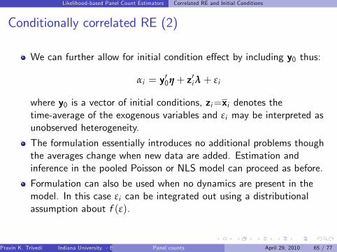
Conditionally correlated RE (2)
We can further allow for initial condition e¤ect by including y0 thus:
αi = y00η+ z0iλ+ εi
where y0 is a vector of initial conditions, zi=xi denotes thetime-average of the exogenous variables and εi may be interpreted asunobserved heterogeneity.
The formulation essentially introduces no additional problems thoughthe averages change when new data are added. Estimation andinference in the pooled Poisson or NLS model can proceed as before.
Formulation can also be used when no dynamics are present in themodel. In this case εi can be integrated out using a distributionalassumption about f (ε).
Pravin K. Trivedi Indiana University. - Bloomington (Prepared for 2010 Mexican Stata Users Group meeting, based on A. Colin Cameron and Pravin K. Trivedi (2005), Microeconometrics: Methods and Applications (MMA), C.U.P. MMA, chapters 21-23 and A. Colin Cameron and Pravin K. Trivedi (2010), Microeconometrics using Stata Revised edition (MUSR), Stata Press. MUSR, chapters 8;18. )Panel counts April 29, 2010 65 / 77

Likelihood-based Panel Count Estimators Correlated RE and Initial Conditions
Dynamic GMM without initial conditionHere individual specic e¤ect is captured by the initial condition
Instruments for equation 1: L.officevis insprv educ age income totchr _cons
/b0 1.447292 .0952543 15.19 0.000 1.633987 1.260597 /xb_totchr .3027348 .0141805 21.35 0.000 .2749415 .330528 /xb_income .0003585 .0004981 0.72 0.472 .0013347 .0006178 /xb_age .1221278 .0134542 9.08 0.000 .0957581 .1484976 /xb_educ .0404143 .0065808 6.14 0.000 .0275162 .0533124 /xb_insprv .2152153 .0331676 6.49 0.000 .1502079 .2802227/xb_L_offi~s .064072 .0041069 15.60 0.000 .0560228 .0721213
Coef. Std. Err. z P>|z| [95% Conf. Interval] Robust
(Std. Err. adjusted for 9861 clusters in dupersid)
Initial weight matrix: Unadjusted Number of obs = 69027Number of moments = 7Number of parameters = 7
GMM estimation
Iteration 6: GMM criterion Q(b) = 7.264e25Iteration 5: GMM criterion Q(b) = 3.032e12Iteration 4: GMM criterion Q(b) = 6.508e06Iteration 3: GMM criterion Q(b) = .01045573Iteration 2: GMM criterion Q(b) = 1.4832673Iteration 1: GMM criterion Q(b) = 4.7296297Iteration 0: GMM criterion Q(b) = 4.9539327Step 1
> instruments(L.officevis insprv educ age income totchr) onestep vce(cluster dupersid). gmm (officevis exp(xb:L.officevis insprv educ age income totchr+b0)), ///
Pravin K. Trivedi Indiana University. - Bloomington (Prepared for 2010 Mexican Stata Users Group meeting, based on A. Colin Cameron and Pravin K. Trivedi (2005), Microeconometrics: Methods and Applications (MMA), C.U.P. MMA, chapters 21-23 and A. Colin Cameron and Pravin K. Trivedi (2010), Microeconometrics using Stata Revised edition (MUSR), Stata Press. MUSR, chapters 8;18. )Panel counts April 29, 2010 66 / 77
Likelihood-based Panel Count Estimators Correlated RE and Initial Conditions
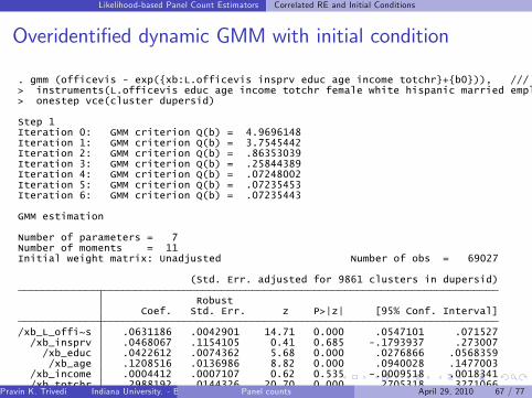
Overidentied dynamic GMM with initial condition
_consInstruments for equation 1: L.officevis educ age income totchr female white hispanic married employed
/b0 1.361726 .0972536 14.00 0.000 1.55234 1.171113 /xb_totchr .2988192 .0144326 20.70 0.000 .2705318 .3271066 /xb_income .0004412 .0007107 0.62 0.535 .0009518 .0018341 /xb_age .1208516 .0136986 8.82 0.000 .0940028 .1477003 /xb_educ .0422612 .0074362 5.68 0.000 .0276866 .0568359 /xb_insprv .0468067 .1154105 0.41 0.685 .1793937 .273007/xb_L_offi~s .0631186 .0042901 14.71 0.000 .0547101 .071527
Coef. Std. Err. z P>|z| [95% Conf. Interval] Robust
(Std. Err. adjusted for 9861 clusters in dupersid)
Initial weight matrix: Unadjusted Number of obs = 69027Number of moments = 11Number of parameters = 7
GMM estimation
Iteration 6: GMM criterion Q(b) = .07235443Iteration 5: GMM criterion Q(b) = .07235453Iteration 4: GMM criterion Q(b) = .07248002Iteration 3: GMM criterion Q(b) = .25844389Iteration 2: GMM criterion Q(b) = .86353039Iteration 1: GMM criterion Q(b) = 3.7545442Iteration 0: GMM criterion Q(b) = 4.9696148Step 1
> onestep vce(cluster dupersid)> instruments(L.officevis educ age income totchr female white hispanic married employed) ///. gmm (officevis exp(xb:L.officevis insprv educ age income totchr+b0)), ///
Pravin K. Trivedi Indiana University. - Bloomington (Prepared for 2010 Mexican Stata Users Group meeting, based on A. Colin Cameron and Pravin K. Trivedi (2005), Microeconometrics: Methods and Applications (MMA), C.U.P. MMA, chapters 21-23 and A. Colin Cameron and Pravin K. Trivedi (2010), Microeconometrics using Stata Revised edition (MUSR), Stata Press. MUSR, chapters 8;18. )Panel counts April 29, 2010 67 / 77

Likelihood-based Panel Count Estimators Correlated RE and Initial Conditions
Dynamic Just Identied GMM with Initial Conditions
Instruments for equation 1: L.officevis T0officevis insprv educ age income totchr _cons
/b0 1.484486 .0605323 24.52 0.000 1.603127 1.365845 /xb_totchr .2847798 .010334 27.56 0.000 .2645256 .3050341 /xb_income .0003019 .0004701 0.64 0.521 .0012232 .0006194 /xb_age .1303702 .0095834 13.60 0.000 .111587 .1491534 /xb_educ .0382539 .0056386 6.78 0.000 .0272024 .0493054 /xb_insprv .2153361 .0351702 6.12 0.000 .1464038 .2842684/xb_T0offi~s .0311947 .0043446 7.18 0.000 .0226794 .0397099/xb_L_offi~s .0495929 .0044248 11.21 0.000 .0409204 .0582654
Coef. Std. Err. z P>|z| [95% Conf. Interval] Robust
(Std. Err. adjusted for 9861 clusters in dupersid)
Initial weight matrix: Unadjusted Number of obs = 69027Number of moments = 8Number of parameters = 8
GMM estimation
Final GMM criterion Q(b) = 6.30e26
> instruments(L.officevis T0officevis insprv educ age income totchr) onestep vce(cluster dupersid) nolog. gmm (officevis exp(xb:L.officevis T0officevis insprv educ age income totchr+b0)), ///
Pravin K. Trivedi Indiana University. - Bloomington (Prepared for 2010 Mexican Stata Users Group meeting, based on A. Colin Cameron and Pravin K. Trivedi (2005), Microeconometrics: Methods and Applications (MMA), C.U.P. MMA, chapters 21-23 and A. Colin Cameron and Pravin K. Trivedi (2010), Microeconometrics using Stata Revised edition (MUSR), Stata Press. MUSR, chapters 8;18. )Panel counts April 29, 2010 68 / 77

Likelihood-based Panel Count Estimators Correlated RE and Initial Conditions
Dynamic Over Identied GMM with Initial Condition
married employed _consInstruments for equation 1: L.officevis T0officevis educ age income totchr female white hispanic
/b0 1.408679 .0607941 23.17 0.000 1.527833 1.289525 /xb_totchr .2805608 .0101571 27.62 0.000 .2606532 .3004684 /xb_income .0004368 .000703 0.62 0.534 .0009411 .0018148 /xb_age .1299791 .0098075 13.25 0.000 .1107567 .1492014 /xb_educ .0402952 .0059253 6.80 0.000 .0286819 .0519085 /xb_insprv .0565968 .1135886 0.50 0.618 .1660328 .2792264/xb_T0offi~s .0305356 .0044538 6.86 0.000 .0218063 .0392648/xb_L_offi~s .0490201 .0046062 10.64 0.000 .039992 .0580481
Coef. Std. Err. z P>|z| [95% Conf. Interval] Robust
(Std. Err. adjusted for 9861 clusters in dupersid)
Initial weight matrix: Unadjusted Number of obs = 69027Number of moments = 12Number of parameters = 8
GMM estimation
Final GMM criterion Q(b) = .0685762
> onestep vce(cluster dupersid) nolog> instruments(L.officevis T0officevis educ age income totchr female white hispanic married employed) ///. gmm (officevis exp(xb:L.officevis T0officevis insprv educ age income totchr+b0)), ///
Pravin K. Trivedi Indiana University. - Bloomington (Prepared for 2010 Mexican Stata Users Group meeting, based on A. Colin Cameron and Pravin K. Trivedi (2005), Microeconometrics: Methods and Applications (MMA), C.U.P. MMA, chapters 21-23 and A. Colin Cameron and Pravin K. Trivedi (2010), Microeconometrics using Stata Revised edition (MUSR), Stata Press. MUSR, chapters 8;18. )Panel counts April 29, 2010 69 / 77
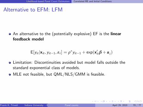
Likelihood-based Panel Count Estimators Correlated RE and Initial Conditions
Alternative to EFM: LFM
An alternative to the (potentially explosive) EF is the linearfeedback model
E[yit jxit , yit1, αi ] = ρyit1 + exp(x0itβ+ αi )
Limitation: Discontinuities avoided but model falls outside thestandard exponential class of models.
MLE not feasible, but QML/NLS/GMM is feasible.
Pravin K. Trivedi Indiana University. - Bloomington (Prepared for 2010 Mexican Stata Users Group meeting, based on A. Colin Cameron and Pravin K. Trivedi (2005), Microeconometrics: Methods and Applications (MMA), C.U.P. MMA, chapters 21-23 and A. Colin Cameron and Pravin K. Trivedi (2010), Microeconometrics using Stata Revised edition (MUSR), Stata Press. MUSR, chapters 8;18. )Panel counts April 29, 2010 70 / 77
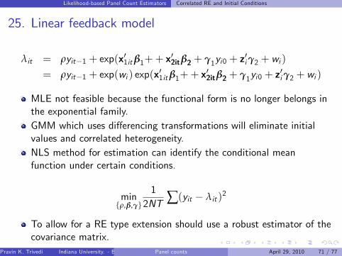
Likelihood-based Panel Count Estimators Correlated RE and Initial Conditions
25. Linear feedback model
λit = ρyit1 + exp(x01itβ1++ x02itβ2 + γ1yi0 + z
0iγ2 + wi )
= ρyit1 + exp(wi ) exp(x01itβ1++ x02itβ2 + γ1yi0 + z
0iγ2 + wi )
MLE not feasible because the functional form is no longer belongs inthe exponential family.GMM which uses di¤erencing transformations will eliminate initialvalues and correlated heterogeneity.NLS method for estimation can identify the conditional meanfunction under certain conditions.
minfρ,β,γg
12NT ∑(yit λit )
2
To allow for a RE type extension should use a robust estimator of thecovariance matrix.
Pravin K. Trivedi Indiana University. - Bloomington (Prepared for 2010 Mexican Stata Users Group meeting, based on A. Colin Cameron and Pravin K. Trivedi (2005), Microeconometrics: Methods and Applications (MMA), C.U.P. MMA, chapters 21-23 and A. Colin Cameron and Pravin K. Trivedi (2010), Microeconometrics using Stata Revised edition (MUSR), Stata Press. MUSR, chapters 8;18. )Panel counts April 29, 2010 71 / 77

Likelihood-based Panel Count Estimators Correlated RE and Initial Conditions
Example: EFM vs LFM
Instruments for equation 1: L.officevis T0officevis insprv educ age income totchr _cons
/b0 2.187085 .096687 22.62 0.000 2.376588 1.997582 /xb_totchr .3270725 .0154421 21.18 0.000 .2968066 .3573383 /xb_income .0002804 .0006164 0.45 0.649 .0014885 .0009277 /xb_age .1234875 .0119579 10.33 0.000 .1000504 .1469245 /xb_educ .0375916 .0062318 6.03 0.000 .0253774 .0498058 /xb_insprv .1509578 .0408185 3.70 0.000 .0709551 .2309606/xb_T0offi~s .0672159 .0038061 17.66 0.000 .0597561 .0746758 /rho .5366234 .0248079 21.63 0.000 .4880008 .585246
Coef. Std. Err. z P>|z| [95% Conf. Interval] Robust
(Std. Err. adjusted for 9861 clusters in dupersid)
Initial weight matrix: Unadjusted Number of obs = 69027Number of moments = 8Number of parameters = 8
GMM estimation
Final GMM criterion Q(b) = 7.35e23
> instruments(L.officevis T0officevis insprv educ age income totchr) onestep vce(cluster dupersid) nolog. gmm (officevis rho*L.officevis exp(xb: T0officevis insprv educ age income totchr+b0)), ///. * Linear Feedback Model with Initial Condition Control
Pravin K. Trivedi Indiana University. - Bloomington (Prepared for 2010 Mexican Stata Users Group meeting, based on A. Colin Cameron and Pravin K. Trivedi (2005), Microeconometrics: Methods and Applications (MMA), C.U.P. MMA, chapters 21-23 and A. Colin Cameron and Pravin K. Trivedi (2010), Microeconometrics using Stata Revised edition (MUSR), Stata Press. MUSR, chapters 8;18. )Panel counts April 29, 2010 72 / 77

Likelihood-based Panel Count Estimators Correlated RE and Initial Conditions
More on LFM vs. EFM
Sensitivity to omitted y0 and z varies between LFM and EFM
Monte Carlo analysis suggests omission leads to biases especially inthe coe¢ cient of lagged variable.
EFM is preferred on predictive performance when the proportion ofzeros is high.
LFM does better when the mean of y is high and proportion of zerossmall.
NLS turns out to be a robust estimator for the LFM. Should beconsidered as a serious alternative for count panel models undercertain conditions.
Pravin K. Trivedi Indiana University. - Bloomington (Prepared for 2010 Mexican Stata Users Group meeting, based on A. Colin Cameron and Pravin K. Trivedi (2005), Microeconometrics: Methods and Applications (MMA), C.U.P. MMA, chapters 21-23 and A. Colin Cameron and Pravin K. Trivedi (2010), Microeconometrics using Stata Revised edition (MUSR), Stata Press. MUSR, chapters 8;18. )Panel counts April 29, 2010 73 / 77

Likelihood-based Panel Count Estimators Correlated RE and Initial Conditions
Concluding Remarks
Much progress in estimating panel count models, especially in dealingwith endogeneity and nonseprable heterogeneity.
Great progress in variance estimation.
RE models pose fewer problems.
For FE models moment-based/IV methods seem more tractable forhandling endogeneity and dynamics. Statas new suite of GMMcommands are very helpful in this regard.
Because FE models do not currently handle important cases, andhave other limitations, CCR panel model with initial conditions, is anattractive alternative, at least for balanced panels.
Pravin K. Trivedi Indiana University. - Bloomington (Prepared for 2010 Mexican Stata Users Group meeting, based on A. Colin Cameron and Pravin K. Trivedi (2005), Microeconometrics: Methods and Applications (MMA), C.U.P. MMA, chapters 21-23 and A. Colin Cameron and Pravin K. Trivedi (2010), Microeconometrics using Stata Revised edition (MUSR), Stata Press. MUSR, chapters 8;18. )Panel counts April 29, 2010 74 / 77

References
Pravin K. Trivedi Indiana University. - Bloomington (Prepared for 2010 Mexican Stata Users Group meeting, based on A. Colin Cameron and Pravin K. Trivedi (2005), Microeconometrics: Methods and Applications (MMA), C.U.P. MMA, chapters 21-23 and A. Colin Cameron and Pravin K. Trivedi (2010), Microeconometrics using Stata Revised edition (MUSR), Stata Press. MUSR, chapters 8;18. )Panel counts April 29, 2010 75 / 77

References
For Count Data magic, if you dont have the Thundercloud,
use instead!
References
A. Colin Cameron and Pravin K. Trivedi (2005), Microeconometrics:Methods and Applications (MMA), C.U.P.(MMA pp.697-740, 743-768)A. Colin Cameron and Pravin K. Trivedi (2009), Microeconometrics usingStata (MUS), Stata Press. MUS pp.229-265, 281-298.Trivedi, P.K. (2010) Recent Developments in Cross section and PanelCount Models. Discussion paper. http://mypage.iu.edu/~trivedi/
Pravin K. Trivedi Indiana University. - Bloomington (Prepared for 2010 Mexican Stata Users Group meeting, based on A. Colin Cameron and Pravin K. Trivedi (2005), Microeconometrics: Methods and Applications (MMA), C.U.P. MMA, chapters 21-23 and A. Colin Cameron and Pravin K. Trivedi (2010), Microeconometrics using Stata Revised edition (MUSR), Stata Press. MUSR, chapters 8;18. )Panel counts April 29, 2010 75 / 77
References
Hausman, J.A., B.H. Hall and Z. Griliches (1984), Econometric Modelsfor Count Data With an Application to the Patents-R and DRelationship,Econometrica, 52, 909-938.Chamberlain, G. (1984). Panel Data. In Handbook of Econometrics,Volume II, ed. by Z. Griliches and M. Intriligator, 1247-1318. Amsterdam:North-Holland.Wooldridge, J. (2005). Simple solutions to the initial conditions problemin dynamic, nonlinear panel data models with unobserved heterogeneity.Journal of Applied Econometrics, 20, 39-54.
Pravin K. Trivedi Indiana University. - Bloomington (Prepared for 2010 Mexican Stata Users Group meeting, based on A. Colin Cameron and Pravin K. Trivedi (2005), Microeconometrics: Methods and Applications (MMA), C.U.P. MMA, chapters 21-23 and A. Colin Cameron and Pravin K. Trivedi (2010), Microeconometrics using Stata Revised edition (MUSR), Stata Press. MUSR, chapters 8;18. )Panel counts April 29, 2010 76 / 77

References
Chernozhukov, V; Fernandez-Val, I.; Kowalski, AE (2009) CensoredQuantile Instrumental Variable Estimation viaControl Functions. Discussion paper.Koenker, R. (2004) Quantile regression for longitudinal data. Journal ofMultivariate Analysis 91, 74 89Mundlak, Y. (1978). On the Pooling of Time Series and Cross SectionData. Econometrica, 46, 69-85.Stata Release 11 ManualsWindmeijer, F.A.G. (2008), GMM for Panel Count Data Models, ch.18in L. Matyas and P. Sivestre eds., The Econometrics of Panel Data,Springer.
Pravin K. Trivedi Indiana University. - Bloomington (Prepared for 2010 Mexican Stata Users Group meeting, based on A. Colin Cameron and Pravin K. Trivedi (2005), Microeconometrics: Methods and Applications (MMA), C.U.P. MMA, chapters 21-23 and A. Colin Cameron and Pravin K. Trivedi (2010), Microeconometrics using Stata Revised edition (MUSR), Stata Press. MUSR, chapters 8;18. )Panel counts April 29, 2010 77 / 77


