
Redistricting & the Quantitative Anatomy of a Section 2 Voting
Rights Case
Megan A. Gall, PhD, GISP
Lawyers’ Committee for Civil Rights Under Law
@DocGallJr

Fundamentals
• Decennial Census – counting every person
• Reapportionment – distributing the 435 seats in the US House of Representatives
• Redistricting – dividing populations into districts

Origins of Redistricting Criteria
• Federal requirements
• State adopted ‘traditional redistricting principles’
• The Voting Rights Act of 1965 and race
• Local groups
• The role of partisanship

U.S. Constitution
• U.S. Congressional districts, Baker v. Carr (1962), and the Apportionment Clause in Article 1, Section 2
• State legislative districts, Reynolds v. Sims (1964), and the Equal Protection Clause of the 14th Amendment
• A nuanced difference– Wesberry v. Sanders (1964) – Congressional district
populations must be as equal as is ‘practicable’
– Reynolds v. Sims (1964) – State legislature district populations must be ‘substantially equal’

Equal Population• ‘Ideal district population’ = total population / # of
districts
• Deviations – relative overall mathematical range
• Ideal population = 714– Largest district: 728 people, a + 2% deviation from the
ideal
– Smallest district: 700 people, a -2% deviation from the ideal
– Overall range of 4%

Equal Population Continued
• Local districts• Alternatives to total population
– Evenwel v. Abbott (2016)– State alternatives
• California, Delaware, Maryland, and New York exclude non-resident prisoners
• Kansas excludes non-resident students• Washington excludes nonresident military • Nebraska excludes aliens and Maine excludes non-
naturalized citizens • Hawaii only uses permanent citizens

Traditional Redistricting Principles
• Compactness
• Contiguity
• Preservation of Political Subdivisions
• Preservation of Communities of Interest
• Preservation of District Cores
• Protection of Incumbents
• Other Rules

Compactness map
• Judicially recognized in
Shaw v. Reno (1993)
• Geographic compactness
• Few jurisdictions define
compactness

Contiguity map
• Judicially recognized in
Shaw v. Reno (1993)
• Districts can’t be in
geographically separate
pieces
• Relatively easy and
non-controversial

Preservation of political boundaries map
• Judicially recognized in
Shaw v. Reno (1993)
• Political boundaries,
e.g. counties, cities,
wards
• Not always clear cut
• Splitting jurisdictions

Presevation of COIs map
• Judicially recognized in
Abrams v. Johnson
(1997)
• Groups with similar
geography, social
interactions, trade,
interests, or political
ties
• Non-racial
communities of
interest
• A subjective concept

Presevation of district cores map
• Judicially recognized in
Abrams v. Johnson
(1997)
• Preserving prior district
cores

• Judicially recognized in
Abrams v. Johnson
(1997)
• Exactly what it sounds
like
• Only principle that is
prohibited in some
areas

Other rules
• Sub-county rules
– City Councils, Advisory Boards, County Commissions, Citizen Groups
– Must be pursuant to state and federal laws
– Don’t carry same force of law
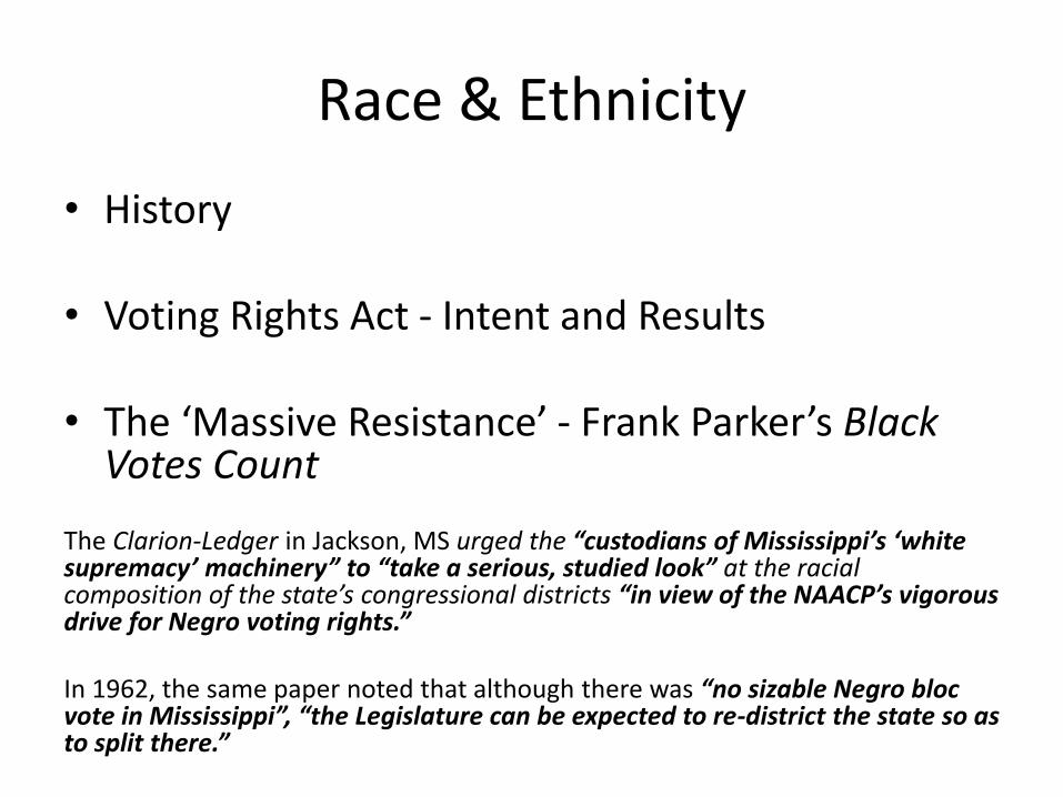
Race & Ethnicity
• History
• Voting Rights Act - Intent and Results
• The ‘Massive Resistance’ - Frank Parker’s Black Votes Count
The Clarion-Ledger in Jackson, MS urged the “custodians of Mississippi’s ‘white supremacy’ machinery” to “take a serious, studied look” at the racial composition of the state’s congressional districts “in view of the NAACP’s vigorous drive for Negro voting rights.”
In 1962, the same paper noted that although there was “no sizable Negro bloc vote in Mississippi”, “the Legislature can be expected to re-district the state so as to split there.”


Establishing Results & Intent
• Thornburg v. Gingles (1986)
– First application of VRA 1982 Amendment
– “…the ability of… cohesive groups of black voters to participate equally in the political process and to elect candidates of their choice” was impaired
– Established a legal framework for assessing claims called the Gingles Preconditions

Gingles Preconditions in Legalese
• “First, the minority group must be able to demonstrate that it is sufficiently large and geographically compact to constitute a majority in a single-member district.”
• “Second, the minority group must be able to show that it is politically cohesive.”
• “Third, the minority must be able to demonstrate that the white majority votes sufficiently as a bloc to enable it – in the absence of special circumstances, such as the minority running unopposed – usually to defeat the minority’s preferred candidate.”

Gingles 1
• Is the racial or language minority ‘sufficiently numerous’ and ‘compact’ enough to form a ‘majority-minority’, single-member district?
– ‘sufficiently numerous’
– ‘compact’
– ‘majority-minority’ district
• 50% + 1 VAP from Bartlett v. Strickland (2009)
– ‘minority’

Data Requirements
• Decennial Census geography and demographics
– Census block level data and geography – building blocks for map-makers
• Data for compliance on other principles

Gingles 2 & 3
• Racially Polarized Voting (RPV) exists when racial/ethnic groups vote as distinct groups with distinct candidate preferences
• Gingles 2: Is voting racially polarized? If so, who are the candidates of choice?
• Gingles 3: Are the minority voters’ candidates of choice usually defeated?
– All questions speak to racial bloc voting, are assessed with the same set of measures, and must be answered affirmatively.

Racially Polarized Voting (RPV)
• The secret ballot
• Available statistical methods
– Homogenous precincts
– Bivariate ecological regression
– EI 2 x 2 (King, 1997)
– EI R x C (Rosen, et al. 2001)

Data Requirements
• Three pieces of data required (all at the voting precinct level of geography)– Candidate vote totals– Candidate race/ethnicity, Party ID, incumbency, & other
notes– Electorate by race/ethnicity
Turnout
Registration
Voting Age Population

Homogeneous Precincts
• Primitive
• Makes a lot of ‘assumptions’
• Relies on existence of homogeneous precincts
• Great for eye-balling data

Ecological Regression (ER)
• Bivariate regression
• Summarizes relationship between two variables: racial/ethnic composition of the precinct and votes cast for a candidate in the precinct
• Using data from all precincts
• Can give unrealistic resultsCandidate A Candidate B
Black Support 5% 90%
White Support 80% 15%

Ecological Inference (EI)
• Developed by Gary King in 1997 in A Solution to the Ecological Inference Problem
• Process of inferring individual-level behavior from aggregate-level data
• Incorporates ‘method of bounds’ (Duncan and Davis 1953)
• Uses bounds with maximum likelihood estimator
• One EI statistic provides minority and ‘other’ vote estimates for a single candidate
• Results are estimates Candidate A Candidate B
Black Support 5% 90%
White Support 80% 15%

EI R x C
• Developed by Rosen, Jiang, King, and Tanner in 2001 in Bayesian and frequentist inference for ecological inference: the R x C case
• EI R x C provides estimates of support for multiple groups for a single candidate
• Bayesian Multinomial-Direchlet hierarchical model
• Better model for contest with more than 2 race/ethnic groups
• Not yet widely used
• Computational demands

Source: http://nationalatlas.gov
The Legal Balancing Act

The 2020 Decennial Census
Participate!

Megan A. Gall, PhD, GISP
@DocGallJr
Intro to GIS Distance Analyses:
https://github.com/MeganGall/Tufts_GIS


