
1
Regression Analysis in the Market Approach:
Using the Gordon Model as a Guide to
Selection of Independent Variables
©2012 Jay B. Abrams, ASA, CPA, MBA
Contents Introduction ..................................................................................................................................... 2
Confessions of a Reformed Quant .............................................................................................. 2
Theoretical Relationships between FMV and Valuation Drivers ................................................... 2
Definitions................................................................................................................................... 3
Mathematical Derivation of Valuation Formulas and Ratios ..................................................... 5
Risk ......................................................................................................................................... 6
Factors Determining Value and the P/E Multiple ................................................................... 8
The P/S Multiple ..................................................................................................................... 9
Consider Using Squared Variables and Logs ........................................................................... 10
Advantage of Scaled Variables as the Dependent Variable ...................................................... 10
Which Variables Must Be Statistically Significant? ................................................................. 11
Regression Examples .................................................................................................................... 11
Table 1 ...................................................................................................................................... 12
Tables 2 and 3 ........................................................................................................................... 13
Tables 4 and 5 ........................................................................................................................... 16
Tables 6 and 7 ........................................................................................................................... 16
Conclusion .................................................................................................................................... 17
Regression Tables 1 – 7 ................................................................................................................ 19
Table 1: Regression Data ......................................................................................................... 20
Table 2: Regression Data ......................................................................................................... 22
Table 3: Regression of P/S ....................................................................................................... 25
Table 4: Regression Data ......................................................................................................... 27
Table 5: Regression of P/S ....................................................................................................... 28
Table 6: Regression Data ......................................................................................................... 29
Table 7: Regression of P/S ....................................................................................................... 32

2
Introduction
Regression analysis is a statistical technique to measure the mathematical relationship between a
dependent variable and one or more independent variables. In the context of the Market
Approach in business valuation, the dependent variable is usually some variation of Fair Market
Value (FMV), i.e., market capitalization in the Guideline Public Company method, selling price
(IBA), or MVIC (Market Value of Invested Capital, Pratt’s Stats). We can use the dependent
variable in dollars or as a scaled variable, i.e., divided by sales, earnings, EBIT, etc.
Confessions of a Reformed Quant
I have used regression analysis in valuation ever since I started in the valuation profession in
1983. I used it on my very first valuation—of a major motion picture producer—to forecast
syndication revenues as a function of either theatrical revenues or television revenues. (It turned
out that the latter was statistically significant, not the former.)
Regressions are enjoyable to perform, and they can be very powerful. It is much harder to argue
with a well-done regression than with mean or median multiples with subjective adjustments.
One of the great benefits of regression is its objectivity and rich statistical feedback to provide
information on its own reliability.
As regression textbooks tend to be very general, they do not address many issues that are specific
to business valuation. The textbooks give us the basic tools. They tell us how to use the tools,
but not where to use them. Much of what I have learned about using regression analysis has
been from experience—a combination of trial-and-error, seeing what works and what does not,
and thinking about how to do it better.
In my early years I enjoyed regression so much that I was willing to do “the shotgun
approach”—regressing the dependent variable(s) against 100+ independent variables. Even for a
quant like me, eventually this became tiring and is very unprofitable on fixed fee assignments.
There had to be a better way.
Eventually I realized the need to develop a theoretical model as a guide to tell me where to look
for independent variables and—equally as important—where not to look.
Theoretical Relationships between FMV and Valuation Drivers
In this article we develop the theoretical relationship that should exist between FMV and the
valuation drivers, i.e., the independent variables that affect value, e.g., income, cash flow, risk,
growth, etc. The importance of doing so is:

3
(1) To reduce the risk of data mining, which is finding apparently statistically significant1
relationships that are in reality the result of chance through brute force regression
analysis of many dozens of variables.
(2) To save time by not having to test independent variables that should have no theoretical
relationship to FMV.
The Gordon model multiple is the logical place to start, as it is the value equation of a mature
firm. Before diving into it, let’s begin with some algebraic definitions.
Definitions
C Cash
CF Cash Flow Available for Dividends
CM Contribution Margin = Sales – Variable Costs
D Debt
Depr Depreciation Expense
DOL Degree of Operating Leverage:2 FCVCS
VCS
NOI
CMDOL
E Earnings = Net Income
Eqy Equity
FC Fixed Costs
1 In statistical significance testing, the p-value (or simply p) is the probability of obtaining a test statistic at least as
extreme as the one that was actually observed, assuming that the null hypothesis is true. In regression analysis, the null
hypothesis is that the true value of the x-coefficient or y-intercept is zero. The smaller the p-value, the more strongly
the test rejects the null hypothesis, that is, the hypothesis being tested. One normally rejects the null hypothesis when
the p-value is less than the significance level α (Greek alpha). It is standard procedure to accept as statistically
significant all variables for which p ≤ 5%. Many authorities routinely accept the statistical significance if p ≤ 10% and
reject variables for which p > 10%. When we reject the null hypothesis, we say that the result is statistically significant.
The y-intercept is not an independent variable. Therefore, its statistical significance or lack thereof is not a reason to
accept or reject a regression. 2 There are different measures and definitions of Operating Leverage that accomplish approximately the same thing.
We do not use this definition later in the article, as we use the one entitled “Operating Leverage” instead; however, this
could be an alternative variable to Operating Leverage.

4
f() A function of
g Long-term growth rate in cash flows available for dividends
g1 Year 1 growth rate in earnings
GFA Gross Fixed Assets = Property Plant & Equipment before Accumulated Depreciation
GMM Gordon Model multiple. The midyear GMM3 = gr
r
1
Int Interest Expense
NFA Net Fixed Assets = Property Plant & Equipment less Accumulated Depreciation
NOI Net Operating Income = S – VC – FC
OL Operating Leverage = FC / VC
P Price, i.e., the selling price of the company. This variable can be a little tricky, because
in the context of the Guideline Public Company Method, it means the market cap—a type
of FMV—of the public Guideline Companies, which includes all necessary net working
capital. However, with respect to the IBA data,4 the selling price excludes cash,
receivables, and debt and is not FMV and requires adjustments to calculate it. This
distinction should be clear in context of each discussion below.
P/E Price-to-Earnings Ratio = Price / Earnings
PM Profit Margin = E / S
POR Payout Ratio = Cash Flow Available for Dividends / Net Income
P/S Price-to-Sales Ratio = Price / Sales
3 Quantitative Business Valuation: A Mathematical Approach for Today’s Professionals, 2
nd Edition, Jay B. Abrams,
John Wiley & Sons, 2010, equation (4.10e), p. 93. 4 The same is often true of Pratt’s Stats. However, Pratt’s Stats is not as rigorous as the IBA in controlling the
definition and calculation of price, which leads to less reliability. Additionally, in recent years, Pratt’s Stats switched to
using MVIC as its primary measure of deal price, and MVIC has additional problems that I may address in a future
article.

5
r Discount Rate
S Sales
t Time, usually measured in years. In valuation, we usually denote t = 0 to mean the
valuation date. The valuation date is a point in time—just like balance sheet items.
However, income statement items and cash flows occur across spans of time. Year t is
the time period from t – 1 to t, and year t + 1 means the first forecast year (from time t to t
+ 1). The context should make it clear whether we refer to a point in time or a span of
time.
TA Total Assets
TC Total Costs = FC + VC
VC Variable Costs
Mathematical Derivation of Valuation Formulas and Ratios
For a mature firm, i.e., a firm for which we forecast constant growth forever, FMV (or the Price)
equals the first year’s forecast cash flow multiplied by the Gordon Model multiple.
(1) gr
rCFP tt
11
Equation (2) states that cash flow equals earnings multiplied by the Payout Ratio.
(2) PORECF
Substituting equation (2) into equation (1), we get:5
(3) gr
rPOREP tt
11
Forecast earnings in year t+1, Et+1, are equal to prior year earnings, Et (or, more simply, E),
multiplied by one plus the Year 1 growth rate, g1. Substituting this into equation (3), we get:
5 In this article, we assume that POR remains fixed over time.

6
(4) gr
rPORgEP
1)1( 1
Thus, we expect that firm value or selling price is a function of the Year 1 growth rate of
earnings, the Payout Ratio, the discount rate (a measure of risk), and the long-term growth rate of
cash flows available for dividends. The Payout Ratio is negatively related to growth. Faster
growth requires retaining a greater percentage of net income than slow growth. So, the Payout
Ratio itself is a function of growth.
We can summarize the essential relationship in equation (5) as price (or FMV) is a function of
earnings, risk, and growth.6
(5) P = f(earnings, risk, and growth)
Risk
Risk is a function of the following factors:
(1) Industry
(2) Size, with small firms being riskier than large firms
(3) Operating leverage
(4) Company volatility
(5) Financial leverage
(6) Cash
(7) Other unknown factors
Industry
While industry is typically a risk factor, we normally select only firms from one industry for our
regression analysis. Therefore, industry is not normally an independent variable in our
regressions.
The exception to this occurs when there are important and well-defined industry niches, in which
case we use dummy variables (1 if true, 0 if false) to measure the effects of niche. For example
in restaurants, there are white tablecloth restaurants, burger restaurants, etc. It is a good idea to
test if restaurant type is significant in the pricing with a dummy variable. Additionally, it is
important to test if franchise names are significant. Several years ago I found that Burger Kings
6 Thus, the GMM guides us in regression analysis by showing us that price is a function of earnings, risk, and growth.
However, we do not actually derive all of the regression independent variables directly from the GMM, as it is merely a
guide.

7
sell for several hundred thousands of dollars more than a generic “Joe’s Burgers” with the same
gross revenues and net income.
Size
We have found that the logarithm of book equity or total assets is often a good proxy for size.
Another good candidate is the net book value of tangible assets, as they have more defensive
value than net book value. The intangible assets are more likely to lose their value than tangible
assets if the company experiences hard times. Using log sales can be problematic, however,
especially when regressing a price-to-sales multiple.7 It is better to avoid having sales on both
sales of the equation.
Operating Leverage8
Firms with high fixed costs and low variable costs, the typical profile being highly automated
manufacturing firms with large investments in fixed assets, should have more variable results
than other firms, because in good times when sales are high, profits are very high, and in bad
times the reverse is true, with high depreciation expense charged against low gross sales. Firms
with lower fixed costs can do more hiring in good times, lay off in bad times, and have more
stable profitability. Thus, high operating leverage is risky, and firms should only undertake it
when the expected increase in average net income is sufficient to offset the additional risk.
The data usually are not readily available to calculate the degree of operating leverage directly
for the guideline companies. It is not always easy to tell which costs are fixed and which are
variable, as the public firms may not provide sufficient detail. However, net fixed assets, gross
fixed assets, or depreciation expense as a percentage of total assets (NFA/TA, GFA/TA, or
Depr/TA) may be reasonable shortcut proxies for operating leverage.
Company Volatility
The standard deviation of operating income (σOp Inc) is a potential measure of risk. There is
likely to be some overlap of this variable with Operating Leverage, yet it is worthwhile to
include as its own variable.
We expect that firms with high Operating Leverage will have a high standard deviation of
income, on average, as the firm experiences good and bad times and sales rise and fall.
However, that may not happen during a long run of good times or bad times, as long as they are
uniformly one or the other. During a 5-year run of only good sales, we would not expect to see
much volatility of earnings arising from high operating leverage, yet the firm may have a high
7 For instance, it can also be problematic when regressing a P/E multiple, as earnings is a function of sales in that it
equals sales times profit margin. 8 There are a number of definitions of Operating Leverage (OL). The analyst could try various measures of OL in a
regression to see which performs best. However, this one should be good enough, and I do not believe it necessary
anymore to try everything under the sun, just because it might be marginally better.

8
volatility of its costs. That is the purpose of including this variable in addition to Operating
Leverage.
Financial Leverage
The following ratios are useful in measuring financial leverage: debt-to-equity ratio (D/Eqy),
debt-to-total assets (D/TA), or interest expense to earnings (Int/E). All things held equal, higher
financial leverage increases risk.
Cash
We have found that the market may care about how much cash in dollars (C) or as a percentage
of total assets (C/TA) the firm has. C/TA can be a statistically significant indicator of risk.
Having sufficient cash to last through difficult times or to take advantage of an opportunity can
be a determinant of risk and value. Nevertheless, the valuation analyst must be cautious with this
variable, as cash may be a result of value, not a cause of it.
Factors Determining Value and the P/E Multiple
Adding in the various factors that determine risk, we expand equation (5) to:
(6) P = f(E; size; FA/TA or Depr/TA; OL; σOp Inc; D/Eqy, D/TA, or Int/E; C/TA; g)
Equation (6) tells us that value is a function of earnings, size;9 fixed assets (net or gross) or
depreciation as a percentage of total assets; operating leverage; the standard deviation of
operating income; a choice of debt-to-equity, debt-to-total assets, or interest expense as a
percentage of earnings; cash/total assets; growth; and, of course, other unknown factors, which
do not appear in the equation.
The best growth figure to use, if possible, is growth in cash flows. However, this is often
impossible to obtain, and we may have to use growth in net income, EBIT, or even sales as a
proxy for growth in cash flows. Similarly, while we ideally should be using profit margin (net
income / sales), often we have to use similar proxies for margin.
We do not generally include the discount rate in a regression, because it is not practical to
calculate or research it for each guideline company, and we have no independent discount rate
for the subject company.
Dividing equation (4) by E, we get:
(7) gr
rPORgEP
1)1(/ 1
9 We mentioned above that size is a measure of risk. It is also the case that size and growth are correlated.
9
Thus, the P/E multiple is a function of risk and growth, or:
(8) P/E = f(size; FA/TA or Depr/TA; OL; σOp Inc; D/Eqy, D/TA, or Int/E; C/TA; g)
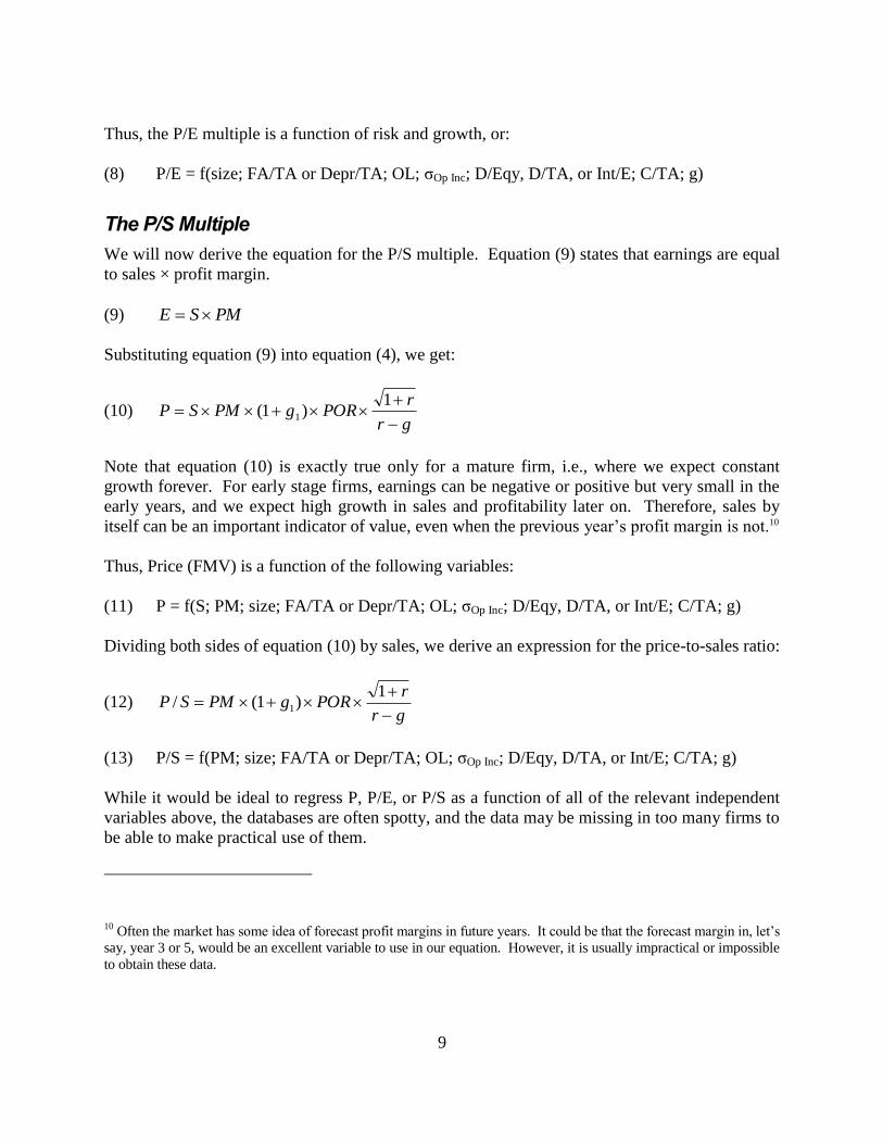
The P/S Multiple
We will now derive the equation for the P/S multiple. Equation (9) states that earnings are equal
to sales × profit margin.
(9) PMSE
Substituting equation (9) into equation (4), we get:
(10) gr
rPORgPMSP
1)1( 1
Note that equation (10) is exactly true only for a mature firm, i.e., where we expect constant
growth forever. For early stage firms, earnings can be negative or positive but very small in the
early years, and we expect high growth in sales and profitability later on. Therefore, sales by
itself can be an important indicator of value, even when the previous year’s profit margin is not.10
Thus, Price (FMV) is a function of the following variables:
(11) P = f(S; PM; size; FA/TA or Depr/TA; OL; σOp Inc; D/Eqy, D/TA, or Int/E; C/TA; g)
Dividing both sides of equation (10) by sales, we derive an expression for the price-to-sales ratio:
(12) gr
rPORgPMSP
1)1(/ 1
(13) P/S = f(PM; size; FA/TA or Depr/TA; OL; σOp Inc; D/Eqy, D/TA, or Int/E; C/TA; g)
While it would be ideal to regress P, P/E, or P/S as a function of all of the relevant independent
variables above, the databases are often spotty, and the data may be missing in too many firms to
be able to make practical use of them.
10
Often the market has some idea of forecast profit margins in future years. It could be that the forecast margin in, let’s
say, year 3 or 5, would be an excellent variable to use in our equation. However, it is usually impractical or impossible
to obtain these data.

10
Consider Using Squared Variables and Logs
It is possible that some of the independent variables may be quadratic or logarithmic and not
simply linear. The profit margin in equation (12) only appears to be linear. However, in
addition to its own direct effect in equation (12), profit margin may operate indirectly as part of
risk.
For example, a business with high volume and a low profit margin may be higher risk than a
lower volume business with a high profit margin. Small changes in the profit margin of the first
company are likely to have a much larger impact than they would have on the second company.
Thus, the valuation analyst might consider having PM and PM2 as independent variables, and the
regression will tell us if either or both are statistically significant.
Advantage of Scaled Variables as the Dependent Variable
A scaled variable is a ratio. Using a scaled dependent variable, either P/S or P/E, has the
advantage of eliminating or at least reducing the statistical problem of heteroscedasticity, which
occurs when the errors in the regression equation are correlated to the size of the independent
variables. This is true because the error terms in the regression of P/S or P/E are less likely to be
related to the size of the firm and are easier to control by adding log size (total assets or book
value) as an independent variable than when we use the price in dollars as the dependent
variable.
However, there are typically two problems that may impede our using a scaled dependent
variable:
(1) Adjusted R2 is often much lower for scaled variables.11 We then look to the standard
error12 of the y-estimate as our guide as to which variable to use. If the standard error is
lower for the scaled variable, we should use that regression, even if its Adjusted R2 is
lower. For example, let’s say that we have two regressions—one with Price as the y-
variable, with a standard error of the y-estimate of $5 million, and the other regression
11
R2 is a measure of the percentage of the total variation in the dependent variable (market capitalization) that is
explained by the independent variables. If there is only one independent variable, the R2 is also the percentage
reduction of forecasting error resulting from forecasting with the regression equation rather than using the average of
the dependent variable. In general, R2 tells us how well the regression explains the variation in the dependent variable.
An R2 of 100% would mean the regression completely explains all variation in the dependent variable. Because
random variation will appear to give some explanatory power to each independent variable, we remove the statistically
expected false explanatory power by adjusting R2 down to adjusted R
2. The larger the sample size, the smaller the
adjustment. 12
The standard error (SE) measures the accuracy of the regression estimate. The larger the standard error, the less sure
we can be about the regression equation’s ability to forecast the dependent variable. An approximate 95% confidence
interval can be formed by doubling the standard error. In other words, we can be approximately 95% sure that the true
value of the dependent variable = its forecast amount ± 2 × SE.

11
with P/E as the y-variable, having a standard error of the y-estimate of 3.0. We would
multiply the standard error, 3.0, by the average earnings of the sample, $1.5 million, for
example, resulting in $4.5 million. Since $4.5 million is less than $5 million, all things
held equal, the P/E-based regression would be preferable.
(2) With the IBA data, there may not be enough data to have an independent variable.
Which Variables Must Be Statistically Significant?
There is another important distinction in regressions with scaled versus absolute variables. In a
regression of an absolute dependent variable, e.g., Price, it is critical that the independent
variables must be statistically significant, while it does not matter if the y-intercept is statistically
significant.13 That is because it does not make-or-break the regression if the true value of the y-
intercept might be zero instead of the number in the regression. However, you should throw out
any independent variable that is statistically insignificant and rerun the regression until all
independent variables remaining in the regression equation are statistically significant.
In working with scaled dependent variables, if all independent variables are insignificant, it still
matters if the y-intercept is statistically significant. Let’s consider an example. Suppose our
regression equation is P/E = 3.0 + 1.2 PM, but the x-coefficient for profit margin is statistically
insignificant. If the y-intercept is statistically significant, then it means that the average Price-
Earnings ratio of the observations is likely to be a valid forecast of value, as we can reject the
null hypothesis that P/E = 0.
Regression Examples
It is instructive to go through some examples. These examples came from actual assignments
that I have done. The Guideline Company data are actual, while the subject company data are
not.
We organize the tables as follows. Table 1 is self-contained, i.e., the data and the regression
appear in the same table, because there are so few observations. For the remaining tables, we
first present the data in one table and the regression of that data in the following table. To make
it easy to distinguish between the data for the dependent and the independent variables, we
highlight the former in green and the latter in tan.
My goal is to show my thinking process in how to understand and analyze regression analysis.
The more I use regression, the more it is clear to me that it is an art that sits on top of a science.
13
Of course, if the y-intercept and all independent variables are statistically insignificant, then the regression has
succeeded in demonstrating that nothing explains prices, i.e., they appear to be random. Fortunately, this is an
extremely rare occurrence. The only time I recall this happening is in my 2008 regression of discounts in the
Partnership Profiles database. This clearly came about as a result of the market being in total disarray during the height
of the Financial Crisis.

12
There is much science in regression analysis—mainly in the mathematics and statistics, which I
have largely not addressed in this article—but regression also has much art. It requires creativity
and judgment. While Excel may do the mechanical calculations for you, it is anything but a
mindless, mechanical exercise. Those who make it so are mere technicians—and not very good
ones at that. To be a scientist is to be an artist.
Table 1
In Table 1, we regressed P/S as function of 3 x-variables: ln(Assets),14 ln(CAGR Sales),15 and
Profit Margin squared, where ln is the natural logarithm. Our x-variables are three of those in
equation (13)—Ln(Assets) is a measure of size, Ln(CAGR Sales) is a measure of growth, and
Profit Margin squared is a measure of profit margin.
The regression has an adjusted R2 of 99% (B17) and each x-variable has a statistically significant
p-value of less than 5% (E29 to E31). For example, the p-value of Ln(Assets) is 0.029 (E29).
This means there is a 2.9% probability that the true and unknowable x-coefficient of Ln Assets is
really zero, but we would obtain a t-statistic as or more extreme than -5.72 (D29), which means t
≤ -5.72 or t ≥ 5.72. With our p-value of 2.9%, we reject the null hypothesis, conclude that
Ln(Assets) is statistically significant, and keep it in the regression equation.
Using sample data in cells B34 to B37, we determine a regression estimate of the P/S multiple of
3.09 (D44) and a regression estimate of the FMV of $154,357 (D45). However, the regression
suffers from having only 6 observations. Using only one x-variable may be preferable to using
more x-variables in cases with only a few observations, as it preserves more degrees of
freedom.16 Table 2 has more observations.
Let’s analyze the sign of the x-coefficients in B29 to B31. It is negative for log of Assets, which
means the market appears to be pricing smaller firms at higher P/S multiples than larger firms.
This is not necessary intuitive, nor is it an absolute violation of intuition either. Normally we
would think that increasing size should reduce risk and therefore increase rather than decrease
the P/S multiple. Thus, it is normal to think that the x-coefficient is more likely to be positive.
Somehow the market seems to think that the small firms are more valuable per dollar of sales
than the large firms are, with size measured by total assets. One of many possible explanations
for this is that ideally we should be using forecast rather than historical profits and growth.
However, forecasts are not always easily available, and we often must use historical numbers as
proxies for forecasts. This, however, is imperfect, and it could be that the market expects the
smaller firm sales and/or margins to grow faster than the large firms—in particular, more than
14
Where assets means total assets 15
CAGR = compound average growth rate 16
Degrees of freedom equals n – k – 1, where n is the number of observations and k is the number of independent
variables.

13
their history would indicate. In other words, investors may think that small firms will
outperform their history more than large firms will.
The x-coefficients for the log of CAGR for sales and the profit margin are positive, as they
should be. If these x-coefficients had the wrong sign, I would be inclined to distrust the
regression results and probably would discard this regression.
The log CAGR x-coefficient warrants further explanation, as the log mathematics can be a bit
confusing. The compound growth rate in sales is typically a percentage under 100%. In this
sample, it ran from 5% to 39%. The natural logarithm of the number 1 (i.e., 100%) equals zero,
and the log of positive numbers greater than zero but less than one is negative.17 Furthermore,
the smaller the growth rate, the more negative is its log. Thus, as the CAGR of sales increases,
ln(CAGR) increases—by being less negative. Thus, the positive x-coefficient makes sense.
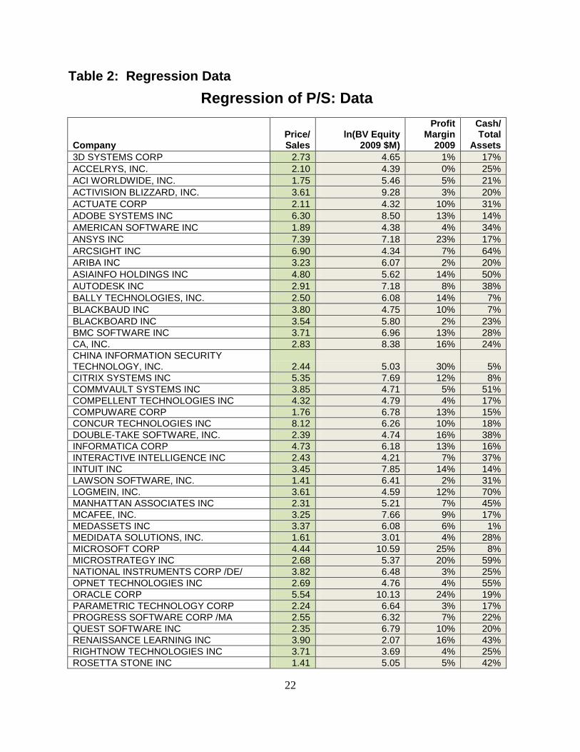
Tables 2 and 3
We will spend more time analyzing these two tables than the rest of them combined. Because
we will spend more time speaking of Table 2 than Table 3, all cell references refer to Table 2
unless we specifically say Table 3.
The Regression
We begin with the data in Table 2 for the regression in Table 3. There are many more companies
in Table 2 than in Table 1. Our sample size is 57 companies, which means that we can rely on
the law of large numbers to interpret our regression statistics. However, the adjusted R2 is only
16.7% (Table 3, B9), which is a bit disappointing. In general, R2 tends to be quite low when the
dependent variable is a ratio, while it is usually much higher when the y-variable is in an absolute
unit such as dollars. The high R2 in Table 1 is extremely unusual.
This regression has 3 x-variables: Ln(2009 BV of Equity in millions), profit margin from 2009,
and cash/total assets. Again, our x-variables are three of those mentioned in equation (13). Note
that the x-coefficients are all positive, as they should be, i.e., we expect that the P/S multiple
should be larger as we increase book value, profit margin, and cash/total assets.
Using sample data in Table 3, B26 to B30, we determine a regression estimate of the P/S
multiple of 3.71 (Table 3, D37) and a regression estimate of the FMV of $296,458,433 (Table 3,
D38).
Percentile Analysis of the Subject & Guideline Companies
Let’s examine Table 2 more closely to inject some intuition into our regression result and why it
is reasonable—or not. The average (i.e., the mean) P/S multiple of our sample is 3.59 (B62), so
17
Because the log of negative numbers is undefined (negative infinity), you cannot use a log transformation of the data
when any of the GCs have negative growth rates—or any negative parameters, for that matter.

14
our regression estimate of 3.71 is only 3% higher than the mean. In other words, it is fairly much
at the mean P/S ratio. Is that a reasonable result? Let’s drill deeper to answer that question.
In rows 65 to 86, we show percentiles—1% and 99% (A66, A86) at the extremes, and 5% to
95% in the middle in 5% increments. In each column B through E, we show where the subject
company data from Table 3, D37 and B33 to B35 falls in the Guideline Company data in bold.
The percentiles are:
1. The Dependent Variable: Our regression-estimated P/S multiple of 3.71 is somewhere
between the 65th
and 70th
percentile (A79, A80), i.e., it is somewhere in between B79 and
B80. In fact, it is in the 67th
percentile (not shown in the table).
a. The mean P/S multiple of 3.59 is in the 62nd
percentile. Thus, the regression
caused us to increase our P/S multiple from our starting point of the mean, which
is in the 62nd
percentile, to the 67th
percentile—an increase of 5 percentile points.
b. Distribution Symmetry
i. When the mean is higher than the median—the latter being the 50th
percentile—the distribution is skewed right, as it is in this case. P/S (and
P/E) multiples are typically skewed right. Usually there are large number
of small P/S multiples and a smaller number of large P/S multiples. The
large ones exert a disproportionate effect on the average, causing it to
increase, while they have less impact on the median.
ii. When the mean P/S multiple is lower than the median, the distribution is
skewed left. This is unusual.
iii. When the mean and median are the same, the distribution is symmetrical.
Normal distributions are symmetrical, although symmetry alone does not
necessarily mean the distribution is normal.
2. The Independent Variables
a. The natural log of 1,000 is 6.9078 (Table 3, B33), which falls between the
numbers in Table 2, C81 and C82. Thus, the subject company ln(book equity) is
between the 75th
and 80th
percentiles and is actually in the 76th
percentile (not
shown).
b. Our subject company has a profit margin of 8% (Table 3, B27 and B34). This
falls between the 45th
and 50th
percentiles in Table 2, between D75 and D76.
More precisely, it is at the 46th
percentile (not shown).
c. Subject company cash of $500,000 (Table 3, B28) divided by total assets of $2
million (B29) leads to cash/total assets of 25% (B35). Turning back to Table 2,
we see that is at the 55th
percentile, i.e., it approximately equals E77.
3. Summary: We have determined that the subject company is in the 76th
, 46th
, and 55th
percentiles, respectively, in its independent variables. The average of the three
percentiles is the 59th
percentile, while our dependent variable, the P/S multiple of 3.71,
is in the 67th
percentile. Our regression-determined P/S multiple seems to be in the
ballpark. To ascertain if this is right, we reconcile the sample mean to the regression

15
estimate. Note: this is not a normal procedure to perform in regression analysis, as it is
implicit in the nature of the technique; however, it is excellent for didactic purposes to do
this once.
Reconciliation of the Sample Mean to the Regression Estimate
Our reconciliation appears in rows 90 to 95. The sample means of the GC independent variables
appear in B90 through B92, transferred from row 62. The subject company data appears in C90
to C92, and the source for these are Table 3, B33 to B35.
Column D is the difference, i.e., columns C – B. For example, the subject company log of book
value is 0.95 (C90 – B90) higher than the GC average.
We multiply the difference in column D by the x-coefficients in column E, transferred from
Table 3, B21 to B23, to calculate the regression’s adjustment to the mean P/S multiple, which is
its starting point. Thus, the adjustment for the log of 2009 book value in millions is 0.95 × 0.36
= 0.34 (F90). Similarly, the subject company’s profit margin of 8.0% (C91) is 1.6% (D91) lower
than the GCs’, which leads to an adjustment of –1.6% × 7.08 = –0.12 (F91). The last adjustment
is for the subject company’s cash/total assets being lower than the GCs’, for an adjustment
of -2.9% × 3.76 = –0.11 (F92).
The sum of the adjustments is 0.12 (F93 = Sum(F90 to F92)). We add this to the GCs’ average
(mean) P/S multiple of 3.59 (F94, transferred from B62) to arrive at the regression-estimated P/S
multiple of 3.71 (F95), which is the sum of F93 and F94 and also equals Table 3, D37.
Thus, we have shown that the regression estimate equals the mean of the dependent variable,
3.59 in this example, plus the sum of the subject company differences multiplied by the x-
coefficients. This is always the case in Ordinary Least Squares regression analysis.
Now we can see why the regression result differs from our average of the three percentiles being
the 59th
percentile. The regression adjustment for the subject and Guideline Company
differences in log 2009 book value in millions is about three times as large as the adjustments for
the differences in each of the other two independent variables, i.e., F90 is about 3 times larger in
absolute value than F91 and F92. The magnitude of the numbers in column F depends on the
size of the differences between subject and guideline companies and the x-coefficient. Even
though the x-coefficients of the other two independent variables are much larger than the x-
coefficient of the log of book value, the larger difference in D90 compared to D91 and D92
more than offsets that effect.
Detail of Difference in Log of Book Values
The purpose of this section is to provide some intuition into the meaning of the 0.95 difference in
the log of book values in D90. It is helpful to know mathematically that natural logs and the
natural exponent (Euler’s constant, e) are inverse functions, i.e., they undo each other. Thus,
ln(ex) = x, and e
ln x = x.
Our subject company has $1 billion in book equity—equal to $1,000 million (B98, transferred
from Table 3, B26). Also, e6.91
= 1,000, i.e., eC90
= B98. Average GC ln(Book Value in Millions)
= 5.96 (B90, transferred from C62). When we exponentiate this, e5.96
= $387.9977 million

16
(B99).18 The ratio of the two numbers is 2.577 (B98/B99 = B100). The log of this number is our
difference of 0.95, i.e., ln(2.577) = 0.95 (B101 = D90).
Tables 4 and 5
We investigate what would happen if we used only 30 observations from Table 2. Table 4 shows
those observations and Table 5 shows the regression. The result is that none of the three x-
variables are significant, as their p-values all exceed 0.10 (Table 5, E21 to E23).
This demonstrates the importance of deciding which data to use. Eliminating one-half of the
data caused the independent variables to become insignificant, although that would not
necessarily be the result in all such cases, as we see in Table 1 that there might be three
statistically significant x-coefficients even with only six observations. With no statistically
significant y-intercept or independent variables, we would conclude the data provide no
meaningful forecasting guidance.
Thus, a biased appraiser can pollute the regression by cherry-picking the data, which can take
two forms: picking only favorable GC data or dropping unfavorable data. In general, it is best to
use all GC data unless there are compelling reasons to drop any of it, and the appraiser should
carefully document the observations dropped and the reasons why. In a litigation context, it is
appropriate to verify opposing expert’s methodology for selecting the GCs and elimination of
observations. It should be methodical and logical, and if it is not, it is fair game for probing and
challenging.
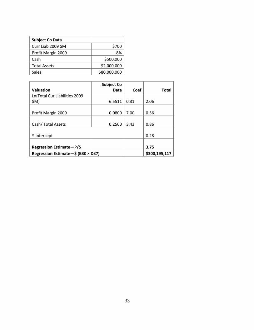
Tables 6 and 7
If we did not have equation (13), we might have chosen log of Total Current Liabilities as an x-
variable. Ln(Total Current Liabilities) is not the best variable to choose as a size variable, nor is
it the best variable to choose as a risk variable. Table 6 contains the same data as Table 2, except
that we replace Ln(BV Equity 2009 $M) with Ln(Total Current Liabilities 2009 $M). Table 7
shows the regression.
While the regression is statistically significant, with all p-values less than 0.10 (Table 7, E21 to
E23), it has a lower adjusted R2, 14.1% (Table 7, B9) than that of Table 3, which was 16.7%
(B9), and its standard error of the y-estimate is higher at 1.90 vs. 1.87 (B10 in both tables).
Additionally, the p-value for ln(Current Liabilities) in Table 7 of 0.099 is materially higher than
the p-value of 0.04 for ln(Book Value) in Table 3.
18
It appears at first glance that the average book value of the Guideline Companies (GCs) is $388 million, but that is
incorrect, because the average of the logs is not the log of the average. A simple example using log base 10 is to work
with the numbers 10 and 1,000, which are 101 and 10
3. Their average is 505. Their base 10 logs are 1 and 3, the
exponents of 10. The average of their logs is 2, yet 102 = 100, which is not 505. Average GC book value is actually
$1.989 billion (not shown).

17
The take-away lesson from these two tables is not to blindly accept statistical significance in a
regression as the end of the story. Statistical significance is a necessary, but not a sufficient
condition in deciding whether or not to use a regression. It is important to use guidance from
valuation theory and common sense in deciding which regressions to use.
To illustrate this point, we repeat the valuation from Table 3 in rows 25 through 38 with the
substitution of ln(current liabilities) for ln(book value). Otherwise, the logic and calculations are
identical to those in Table 3. We come to a valuation of $300.2 million (D38), which is very
close to the value of $296.5 million in Table 3. So far, it appears that there is no material impact
of using the wrong variable. It works—maybe not quite as well as ln book value, but close
enough. Who cares?
However, if the subject company were to have paid off its current liabilities in full,19 which it
could do without affecting its book value of equity, the valuation would decline to $135.4
million (not shown)—a 55% decline in value! Of course, the company may pay off only one-
half of its liabilities, which would give us a different valuation yet. Obviously, it will not do to
have the value of the company vary all over the map with a relatively innocuous decision of how
much of its liabilities are paid on the valuation date. This exposes the underlying weakness of
using the wrong variable. Thus, we observe that sloppy statistics may appear to pass muster—
unless we think and dig deeply.
Conclusion
These theoretical results provide important guidance into which data to test and how to interpret
them in our statistical analysis of the transactional databases and the guideline public company
data. Looking at equation (13) as an example, we have at most 11 independent variables—13 if
we count all three possible variations of size variables—to include in our regression. That is
much faster than trying to regress over 100 independent variables.
Another advantage of using the Gordon model to guide us in limiting our choice of independent
variables is that Excel only allows a maximum of 16 independent variables. While stat programs
do not have this restriction, most appraisers use Excel, and restricting the independent variables
does not force the appraiser to use a stat package. Thus, this approach saves much time and
money.
I end this article with a wish that the readers find it useful, along with a shameless plug that
anyone wishing a more detailed treatment of using regression analysis in valuation consult
19
Since ln(0) is undefined, we would instead change B26 to $1 (representing $1,000), and its natural log is zero.

18
Chapter 3 of Quantitative Business Valuation: A Mathematical Approach for Today’s
Professionals, 2nd
Edition.20 Also, the reader should feel free to call me for help.
20 While the majority of the material in this article appears in the book, this article does contain some new insights that
do not appear in the book. However, chapter 3 of the book is a longer, more detailed treatment of using regression
analysis in valuation.

19
Regression Tables 1 – 7

20
Table 1: Regression Data
Table 1
Regression of P/S--Publicly Traded Software Firms
Company Name P/S Ln Assets Ln CAGR
Sales
Profit Margin
Squared Insightful
Corporation 1.78 9.73 -2.93 0.0083 Synplicity, Inc. 3.15 11.20 -2.02 0.0061 PDF Solutions, Inc. 5.35 11.83 -0.94 0.0014 Ansoft Corporation 5.29 11.11 -2.15 0.0316 Simulations Plus,
Inc. 2.29 8.62 -3.00 0.0031 Vital 6.19 11.30 -1.03 0.0101
SUMMARY OUTPUT
Regression Statistics Multiple R 99.83% R Square 99.67% Adjusted R Square 99.16%
Standard Error 0.17
Observations 6
ANOVA df SS MS F Signif F
Regression 3 16.7783 5.5928 198.7691 0.0050 Residual 2 0.0563 0.0281
Total 5 16.8345
Coef Std Err t Stat P-value Lower 95% Upper 95%
Intercept 18.20
1.96
9.30
0.011
9.78
26.61
Ln Assets (0.87)
0.15
(5.72)
0.029
(1.53)
(0.22)
Ln CAGR Sales 2.92
0.20
14.42
0.005
2.05
3.80
Profit Margin Squared
95.04
8.14
11.67
0.007
59.99
130.08

21
Subject Co Data Assets $30,000
CAGR Sales 10% Profit Margin 8% Sales $50,000
Valuation Subject Co
Data Coefficients Total
Ln Assets 10.3090 (0.87)
(8.98)
Ln CAGR Sales -2.3026 2.92
(6.73)
Profit Margin Squared 0.0064 95.04
0.61
Y-Intercept 18.20
Regression Estimate—P/S 3.09
Regression Estimate—$ (B37 × D44) $154,357
-5.00
0.00
5.00
10.00
15.001
2
3
4
5
6
P/S
Ln Assets
Ln CAGR Sales
Profit Margin Squared
22
Table 2: Regression Data
Regression of P/S: Data
Company Price/ Sales
ln(BV Equity 2009 $M)
Profit Margin
2009
Cash/ Total
Assets
3D SYSTEMS CORP 2.73 4.65 1% 17%
ACCELRYS, INC. 2.10 4.39 0% 25%
ACI WORLDWIDE, INC. 1.75 5.46 5% 21%
ACTIVISION BLIZZARD, INC. 3.61 9.28 3% 20%
ACTUATE CORP 2.11 4.32 10% 31%
ADOBE SYSTEMS INC 6.30 8.50 13% 14%
AMERICAN SOFTWARE INC 1.89 4.38 4% 34%
ANSYS INC 7.39 7.18 23% 17%
ARCSIGHT INC 6.90 4.34 7% 64%
ARIBA INC 3.23 6.07 2% 20%
ASIAINFO HOLDINGS INC 4.80 5.62 14% 50%
AUTODESK INC 2.91 7.18 8% 38%
BALLY TECHNOLOGIES, INC. 2.50 6.08 14% 7%
BLACKBAUD INC 3.80 4.75 10% 7%
BLACKBOARD INC 3.54 5.80 2% 23%
BMC SOFTWARE INC 3.71 6.96 13% 28%
CA, INC. 2.83 8.38 16% 24%
CHINA INFORMATION SECURITY TECHNOLOGY, INC. 2.44 5.03 30% 5%
CITRIX SYSTEMS INC 5.35 7.69 12% 8%
COMMVAULT SYSTEMS INC 3.85 4.71 5% 51%
COMPELLENT TECHNOLOGIES INC 4.32 4.79 4% 17%
COMPUWARE CORP 1.76 6.78 13% 15%
CONCUR TECHNOLOGIES INC 8.12 6.26 10% 18%
DOUBLE-TAKE SOFTWARE, INC. 2.39 4.74 16% 38%
INFORMATICA CORP 4.73 6.18 13% 16%
INTERACTIVE INTELLIGENCE INC 2.43 4.21 7% 37%
INTUIT INC 3.45 7.85 14% 14%
LAWSON SOFTWARE, INC. 1.41 6.41 2% 31%
LOGMEIN, INC. 3.61 4.59 12% 70%
MANHATTAN ASSOCIATES INC 2.31 5.21 7% 45%
MCAFEE, INC. 3.25 7.66 9% 17%
MEDASSETS INC 3.37 6.08 6% 1%
MEDIDATA SOLUTIONS, INC. 1.61 3.01 4% 28%
MICROSOFT CORP 4.44 10.59 25% 8%
MICROSTRATEGY INC 2.68 5.37 20% 59%
NATIONAL INSTRUMENTS CORP /DE/ 3.82 6.48 3% 25%
OPNET TECHNOLOGIES INC 2.69 4.76 4% 55%
ORACLE CORP 5.54 10.13 24% 19%
PARAMETRIC TECHNOLOGY CORP 2.24 6.64 3% 17%
PROGRESS SOFTWARE CORP /MA 2.55 6.32 7% 22%
QUEST SOFTWARE INC 2.35 6.79 10% 20%
RENAISSANCE LEARNING INC 3.90 2.07 16% 43%
RIGHTNOW TECHNOLOGIES INC 3.71 3.69 4% 25%
ROSETTA STONE INC 1.41 5.05 5% 42%

23
SALESFORCE COM INC 8.61 6.51 4% 33%
SKILLSOFT PUBLIC LIMITED CO 3.00 5.32 15% 7%
SMITH MICRO SOFTWARE INC 2.67 5.24 4% 7%
SOLARWINDS, INC. 9.49 4.49 25% 72%
SXC HEALTH SOLUTIONS INC. 1.22 6.13 3% 46%
SYBASE INC 3.19 6.96 14% 38%
SYNOPSYS INC 2.36 7.52 12% 24%
TALEO CORP 4.11 5.82 1% 54%
TELECOMMUNICATION SYSTEMS INC /FA/ 1.16 5.22 9% 13%
TIBCO SOFTWARE INC 2.94 6.68 10% 25%
TYLER TECHNOLOGIES INC 2.27 4.90 9% 4%
VMWARE, INC.
10.38 7.92 10% 49%
WEB.COM GROUP, INC. 1.30 4.64 2% 32%
Average
3.59
5.96 9.6% 27.9%
Standard Deviation
2.05
1.63 6.9% 17.3%
Percentile Price/ Sales
ln(BV Equity 2009 $M)
Profit Margin
2009
Cash/ Total
Assets
1% 1.193 2.596 0.4% 2.3%
5% 1.384 4.110 1.9% 6.3%
10% 1.691 4.364 2.5% 7.4%
15% 1.971 4.530 2.9% 10.3%
20% 2.244 4.663 3.7% 14.2%
25% 2.352 4.755 3.8% 16.6%
30% 2.424 4.878 4.3% 17.3%
35% 2.531 5.148 5.3% 18.5%
40% 2.687 5.269 6.6% 20.1%
45% 2.847 5.495 7.4% 22.2%
50% 2.996 5.821 9.3% 24.1%
55% 3.247 6.080 10.0% 25.2%
60% 3.507 6.226 10.2% 27.6%
65% 3.652 6.440 11.8% 31.6%
70% 3.803 6.644 12.7% 34.1%
75% 3.903 6.794 13.1% 38.2%
80% 4.415 7.135 14.2% 43.2%
85% 5.127 7.603 15.9% 47.8%
90% 6.538 7.874 17.8% 51.9%
95% 8.222 8.653 24.2% 59.7%
99% 9.885 10.331 27.3% 70.8%

24
Reconciliation of Regression Estimate
Independent Variable
Avg GCs
(Row 62)
Subj Co (Table 3, B33:B35)
Difference
= C - B
X-Coef (Table 3, B21:B23)
Adjustment
= D × E
Ln(Book Value in $M)
5.96
6.91
0.95 0.36
0.34
Profit Margin 9.6% 8.0% -1.6% 7.08
(0.12)
Cash/Total Assets 27.9% 25.0% -2.9% 3.76
(0.11)
Total Adjustments
0.12
Guideline Co Average P/S (B62)
3.59
Regr Estimate-P/S (ΣF93:F94=Table 3, D37)
3.71
Detail of Difference in Log Book Values (D90) Subject Company BV in $M (Table 3, B26) 1000
eGC Avg (ln BV) in $M = eC62 [1] 387.9977 Ratio of Book Values (B98/B99) 2.577 Ln Ratio of Values = Ln(B100) = (D90) 0.95
[1] Here we are exponentiating the average of ln(GC BVs). The GC average book value is $1.989 billion, not
$388 million, as it might appear. The log of the average is not equal to the average of the logs. A quick
example using base 10 logs for simplicity is the log of 10 is 1 and the log of 1000 is 3, i.e., 101 = 10,
and 103 = 1000. The average of the logs is 2. However, 102 = 100, not 505, the latter being the average
of 10 and 1000.

25
Table 3: Regression of P/S
Regression of P/S
SUMMARY OUTPUT
Regression Statistics Multiple R 46.0% R Square 21.1% Adjusted R Square 16.7% Standard Error 1.87 Observations 57
ANOVA df SS MS F Signif F
Regression 3 49.707 16.569
4.731 0.005
Residual 53
185.616
3.502
Total 56
235.324
Coef Std Err t Stat
P-value Lower 95%
Upper 95%
Intercept (0.29) 1.21
(0.24)
0.81
(2.71)
2.13
ln(BV Equity 2009 $M) 0.36 0.17 2.12
0.04
0.02
0.70
Profit Margin 2009 7.08 3.80 1.86
0.07
(0.55)
14.71
Cash/Total Assets 3.76 1.53 2.45
0.02
0.69
6.84

26
Subject Co Data BV Equity 2009 $M $1,000 Profit Margin 2009 8% Cash $500,000 Total Assets $2,000,000 Sales $80,000,000
Valuation Subject Co
Data Coef Total
ln(BV Equity 2009 $M) 6.9078 0.36
2.49
Profit Margin 2009 0.0800 7.08
0.57
Cash/Total Assets 0.2500 3.76
0.94
Y-Intercept (0.29)
Regression Estimate—P/S
3.71
Regression Estimate—$ (B30 × D37) $296,458,433

27
Table 4: Regression Data
Regression of P/S: Data
Company Price/ Sales
ln(BV Equity
2009 $M)
Profit Margin
2009
Cash/ Total
Assets
3D SYSTEMS CORP 2.73 4.65 1% 17%
ACCELRYS, INC. 2.10 4.39 0% 25%
ACI WORLDWIDE, INC. 1.75 5.46 5% 21%
ACTIVISION BLIZZARD, INC. 3.61 9.28 3% 20%
ACTUATE CORP 2.11 4.32 10% 31%
ADOBE SYSTEMS INC 6.30 8.50 13% 14%
AMERICAN SOFTWARE INC 1.89 4.38 4% 34%
ANSYS INC 7.39 7.18 23% 17%
ARCSIGHT INC 6.90 4.34 7% 64%
ARIBA INC 3.23 6.07 2% 20%
ASIAINFO HOLDINGS INC 4.80 5.62 14% 50%
AUTODESK INC 2.91 7.18 8% 38%
BALLY TECHNOLOGIES, INC. 2.50 6.08 14% 7%
BLACKBAUD INC 3.80 4.75 10% 7%
BLACKBOARD INC 3.54 5.80 2% 23%
BMC SOFTWARE INC 3.71 6.96 13% 28%
CA, INC. 2.83 8.38 16% 24%
CHINA INFORMATION SECURITY TECHNOLOGY, INC. 2.44 5.03 30% 5%
CITRIX SYSTEMS INC 5.35 7.69 12% 8%
COMMVAULT SYSTEMS INC 3.85 4.71 5% 51%
COMPELLENT TECHNOLOGIES INC 4.32 4.79 4% 17%
COMPUWARE CORP 1.76 6.78 13% 15%
CONCUR TECHNOLOGIES INC 8.12 6.26 10% 18%
DOUBLE-TAKE SOFTWARE, INC. 2.39 4.74 16% 38%
INFORMATICA CORP 4.73 6.18 13% 16%
INTERACTIVE INTELLIGENCE INC 2.43 4.21 7% 37%
INTUIT INC 3.45 7.85 14% 14%
LAWSON SOFTWARE, INC. 1.41 6.41 2% 31%
LOGMEIN, INC. 3.61 4.59 12% 70%
MANHATTAN ASSOCIATES INC 2.31 5.21 7% 45%

28
Table 5: Regression of P/S
Regression of P/S
SUMMARY OUTPUT
Regression Statistics Multiple R 35.1% R Square 12.3% Adjusted R Square 2.2%
Standard Error 1.72
Observations 30
ANOVA df SS MS F Signif F
Regression 3 10.782
3.594
1.219
0.323
Residual 26
76.655
2.948
Total 29
87.437
Coef
Std Err t Stat
P-value
Lower 95%
Upper 95%
Intercept 0.64
1.82
0.35
0.73
(3.09)
4.37
ln(BV Equity 2009 $M)
0.33
0.25
1.35
0.19
(0.17)
0.84
Profit Margin 2009 5.61
4.95
1.13
0.27
(4.57)
15.79
Cash/ Total Assets 1.68
2.15
0.78
0.44
(2.73)
6.09

29
Table 6: Regression Data
Regression of P/S: Data
Company Price/ Sales
Ln(Total Cur
Liabilities 2009 $M)
Profit Margin
2009
Cash/ Total
Assets
Total Cur Liabilities
2009 $M
ln(BV Equity
2009 $M)
3D SYSTEMS CORP
2.73
3.51 1% 17%
33.44
4.65
ACCELRYS, INC.
2.10
4.27 0% 25%
71.61
4.39
ACI WORLDWIDE, INC.
1.75
5.28 5% 21%
195.40
5.46
ACTIVISION BLIZZARD, INC.
3.61
7.83 3% 20%
2,507.00
9.28
ACTUATE CORP
2.11
4.10 10% 31%
60.26
4.32
ADOBE SYSTEMS INC
6.30
6.74 13% 14%
844.55
8.50
AMERICAN SOFTWARE INC
1.89
3.22 4% 34%
24.93
4.38
ANSYS INC
7.39
5.59 23% 17%
266.77
7.18
ARCSIGHT INC
6.90
3.99 7% 64%
53.96
4.34
ARIBA INC
3.23
5.15 2% 20%
172.91
6.07
ASIAINFO HOLDINGS INC
4.80
5.30 14% 50%
200.77
5.62
AUTODESK INC
2.91
6.68 8% 38%
800.10
7.18
BALLY TECHNOLOGIES, INC.
2.50
5.18 14% 7%
178.05
6.08
BLACKBAUD INC
3.80
5.19 10% 7%
180.23
4.75
BLACKBOARD INC
3.54
5.39 2% 23%
218.35
5.80
BMC SOFTWARE INC
3.71
7.20 13% 28%
1,333.30
6.96
CA, INC.
2.83
8.31 16% 24%
4,078.00
8.38
CHINA INFORMATION SECURITY TECHNOLOGY, INC.
2.44
4.33 30% 5%
75.82
5.03
CITRIX SYSTEMS INC
5.35
6.73 12% 8%
834.36
7.69
COMMVAULT SYSTEMS INC
3.85
4.40 5% 51%
81.56
4.71
COMPELLENT TECHNOLOGIES INC
4.32
3.72 4% 17%
41.39
4.79
COMPUWARE CORP
1.76
6.33 13% 15%
561.53
6.78
CONCUR TECHNOLOGIES INC
8.12
4.83 10% 18%
125.10
6.26

30
DOUBLE-TAKE SOFTWARE, INC.
2.39
3.50 16% 38%
32.99
4.74
INFORMATICA CORP
4.73
5.54 13% 16%
255.62
6.18
INTERACTIVE INTELLIGENCE INC
2.43
4.07 7% 37%
58.64
4.21
INTUIT INC
3.45
6.99 14% 14%
1,083.83
7.85
LAWSON SOFTWARE, INC.
1.41
6.08 2% 31%
438.10
6.41
LOGMEIN, INC.
3.61
3.73 12% 70%
41.84
4.59
MANHATTAN ASSOCIATES INC
2.31
4.26 7% 45%
70.95
5.21
MCAFEE, INC.
3.25
7.27 9% 17%
1,436.09
7.66
MEDASSETS INC
3.37
4.60 6% 1%
99.34
6.08
MEDIDATA SOLUTIONS, INC.
1.61
4.54 4% 28%
94.03
3.01
MICROSOFT CORP
4.44
10.20 25% 8%
27,034.00
10.59
MICROSTRATEGY INC
2.68
5.03 20% 59%
152.64
5.37
NATIONAL INSTRUMENTS CORP /DE/
3.82
4.77 3% 25%
118.42
6.48
OPNET TECHNOLOGIES INC
2.69
3.77 4% 55%
43.48
4.76
ORACLE CORP
5.54
9.12 24% 19%
9,149.00
10.13
PARAMETRIC TECHNOLOGY CORP
2.24
6.20 3% 17%
491.43
6.64
PROGRESS SOFTWARE CORP /MA
2.55
5.42 7% 22%
226.92
6.32
QUEST SOFTWARE INC
2.35
5.99 10% 20%
399.96
6.79
RENAISSANCE LEARNING INC
3.90
4.15 16% 43%
63.20
2.07
RIGHTNOW TECHNOLOGIES INC
3.71
4.58 4% 25%
97.31
3.69
ROSETTA STONE INC
1.41
4.19 5% 42%
66.18
5.05
SALESFORCE COM INC
8.61
6.64 4% 33%
766.97
6.51
SKILLSOFT PUBLIC LIMITED CO
3.00
5.50 15% 7%
245.69
5.32
SMITH MICRO SOFTWARE INC
2.67
2.83 4% 7%
16.89
5.24
SOLARWINDS, INC.
9.49
4.14 25% 72%
63.03
4.49
SXC HEALTH SOLUTIONS INC.
1.22
5.21 3% 46%
183.46
6.13
SYBASE INC
3.19
6.82 14% 38%
920.13
6.96

31
SYNOPSYS INC
2.36
6.70 12% 24%
814.59
7.52
TALEO CORP
4.11
4.62 1% 54%
101.67
5.82
TELECOMMUNICATION SYSTEMS INC /FA/
1.16
4.80 9% 13%
121.93
5.22
TIBCO SOFTWARE INC
2.94
5.64 10% 25%
282.18
6.68
TYLER TECHNOLOGIES INC
2.27
4.86 9% 4%
129.25
4.90
VMWARE, INC.
10.38
7.17 10% 49%
1,294.04
7.92
WEB.COM GROUP, INC.
1.30
2.79 2% 32%
16.25
4.64

32
Table 7: Regression of P/S
SUMMARY OUTPUT
Regression Statistics Multiple R 43.3% R Square 18.7% Adjusted R Square 14.1%
Standard Error 1.90
Observations 57
ANOVA df SS MS F Signi F
Regression 3 44.070
14.690
4.071
0.011
Residual 53
191.254
3.609
Total 56
235.324
Coef Std Err t Stat
P-value
Lower 95%
Upper 95%
Intercept 0.28
1.16
0.24
0.813
(2.05)
2.60
Ln(Total Cur Liabilities 2009 $M)
0.31
0.19
1.68
0.099
(0.06)
0.69
Profit Margin 2009 7.00
3.97
1.76
0.084
(0.96)
14.96
Cash/ Total Assets 3.43
1.54
2.23
0.030
0.35
6.51
33
Subject Co Data Curr Liab 2009 $M $700 Profit Margin 2009 8% Cash $500,000 Total Assets $2,000,000 Sales $80,000,000
Valuation Subject Co
Data Coef Total Ln(Total Cur Liabilities 2009
$M) 6.5511 0.31
2.06
Profit Margin 2009 0.0800 7.00
0.56
Cash/ Total Assets 0.2500 3.43
0.86
Y-Intercept 0.28
Regression Estimate—P/S 3.75
Regression Estimate—$ (B30 × D37) $300,195,117


