i
Reliability and economic analysis
of offshore wind power systems-
A comparison of internal grid
topologies
Thesis for the Master of Science Degree (MSc)
Tomas Winter
Department of Energy and Environment
Division of Electric Power Engineering
CHALMERS UNIVERSITY OF TECHNOLOGY
Examiner: Lina Bertling, Professor
Supervisor: Francois Besnard, PhD student
Gothenburg, Sweden, 2011-12-01

ii
Abstract
Wind power has emerged the last decades as an important technology for low carbon emitting
electricity production. The development was first onshore, but recently many wind farms have
been developed offshore due to space availability, low noise and visual impacts. Offshore
wind farms experiences higher winds resulting in higher production, but investment costs, and
operation and maintenance costs are also much higher. More specifically, a failure may result
in long downtime due to inaccessibility to the site during harsh conditions, and transportation
costs are also higher since boats, and sometimes helicopters are necessary.
This study consists of a reliability and economic analysis of the internal grid of offshore wind
power system. Different topologies are evaluated and compared against each other with the
aim of presenting alternative layouts with increased level of reliability at an acceptable cost.
The different layouts are compared in additional income over the life time of the wind farm
considering the energy not supplied.
The results show that for the case study consisting of two arrays of ten 3MW wind turbines–
three of the proposed alternative layouts presents a positive Net Present Value of the extra
investment of 63k€, 165k€ and 201k€ respectively. It can be concluded that it can be
beneficial to implement some degree of redundancy along with improvements in the
protection system.

iii
Table of Contents
ABBREVIATIONS
CHAPTER 1: INTRODUCTION AND BACKGROUND ....................................................... 1
1.1 Background ....................................................................................................................... 1
1.1.1 Why constructing offshore wind power plants? ........................................................ 1
1.1.2 Future wind power initiatives .................................................................................... 1
1.1.3 Reliability analyses .................................................................................................... 2
1.2 Scope of the Work ............................................................................................................ 2
1.3 Method .............................................................................................................................. 3
1.4 Assumptions and scope .................................................................................................... 4
1.5 Previous work in this area ................................................................................................ 4
1.6 Outline of the thesis .......................................................................................................... 5
CHAPTER 2: THEORY ............................................................................................................ 7
2.1 Wind power ...................................................................................................................... 7
2.1.1 Basic of wind energy ................................................................................................. 7
2.1.2 Wind turbines ........................................................................................................... 10
2.2 Net present value and the internal rate of return ............................................................ 13
2.3 Power system reliability ................................................................................................. 14
2.3.1 System analysis ........................................................................................................ 15
2.3.2 Analytical methods and Monte Carlo simulation .................................................... 16
2.3.3 Reliability indices .................................................................................................... 16
2.3.4 Series and parallel systems ...................................................................................... 19
CHAPTER 3: NEPLAN ........................................................................................................... 22
3.1 NEPLAN Planning and Optimization Software ............................................................. 22
3.2 Fundamental Calculation Flow in NEPLAN .................................................................. 22
3.2.1 Network data input ................................................................................................... 23
3.2.2 Generation of failure combination ........................................................................... 23
3.2.3 Overlapping stochastic outages ................................................................................ 24
3.2.4 Failure effect analysis .............................................................................................. 26
3.3 Example cases with NEPLAN and analytical calculations without considering load flow
.............................................................................................................................................. 27

iv
3.3.1 Radial network calculations ..................................................................................... 27
3.3.2 Combination of series and parallel network calculations ........................................ 29
CHAPTER 4: OFFSHORE WIND FARM GRID TOPOLOGY ............................................. 32
4.1 Different layouts for offshore collector systems/Common grid topology structures ..... 32
4.1.1 Radial design ............................................................................................................ 33
4.1.2 Single-sided ring and shared ring design ................................................................. 34
4.1.3 Double-sided ring ..................................................................................................... 34
4.1.4 Star design ................................................................................................................ 35
4.1.5 Single return- or shared ring design ......................................................................... 36
4.1.6 Double-sided half-ring design .................................................................................. 36
4.2 Thanet offshore wind farm ............................................................................................. 37
4.2.1 Basic information and location ................................................................................ 37
4.2.2 Turbines technical specifications ............................................................................. 38
4.2.3 Internal networks technical specifications ............................................................... 39
CHAPTER 5: ANALYSIS OF DIFFERENT TOPOLOGIES ................................................ 41
Alternative layout, Top.1 ...................................................................................................... 43
Alternative layout, Top.2 ...................................................................................................... 44
Alternative layout, Top.3 ...................................................................................................... 45
Alternative layout, Top.4 ...................................................................................................... 46
Alternative layout, Top.5 ...................................................................................................... 46
Alternative layout, Top.6 ...................................................................................................... 47
Alternative layout, Top.7 ...................................................................................................... 48
CHAPTER 6: RESULTS ......................................................................................................... 48
6.1 Description of the results per topology ........................................................................... 48
6.2 Results discussion ........................................................................................................... 53
CHAPTER 7: CONCLUSIONS ............................................................................................... 55
7.1 Conclusions and discussion ............................................................................................ 55
7.2 Future work ..................................................................................................................... 55
REFERENCES ......................................................................................................................... 57

v
Abbreviations
EWEA European Wind Energy Association HL Hierarchical Levels
FF Failure Frequency [1/year]
FD Failure Duration [hours/year]
SAIFI System Average Interruption Frequency Index [int./year,customer]
SAIDI System Average Interruption Duration Index [hour/year,customer]
CAIDI Customers Average Interruption Duration Index [hour/int.]:
ASAI Average Service Availability Index [%]
ENS Energy Not Supplied [MWh/year]
NPV Net Present Value [k€]
IRR Internal Rate of Return [%]
AEAE Additional Expected Annual Energy [MWh/year]
AEI Additional Expected Income [k€]
WACC Weighted Average Cost of Capital [%]
DFIG Double Fed Induction Generator
WRIG Wound Rotor Induction Generator
O&M Operations & Maintenance

1
CHAPTER 1: INTRODUCTION AND BACKGROUND
1.1 Background
The wind power industry is growing rapidly and more wind power plants are being erected
offshore with increasing distance to land. Building wind farms offshore is expensive and
associated with high maintenance cost. Thus there is a growing interest in performing
reliability assessments during the design phase which is the most influential phase for the
O&M. This is performed in order to optimize the topology according to its expected economic
benefits due to less interruption in energy production. The offshore environment and many of
the products are also rather unproved which makes it important to carefully carry out a
reliability assessment in order to avoid trial and errors in most possible way. Despite these
issues offshore wind power plants also comes with several benefits like higher power
production due to stronger winds along with less disturbances to people.
By comparing different topologies of a wind farm it is possible to determine and evaluate the
most reliable installation. The reliability study can also highlight weak points within the
system which might need improvements in redundancy.
A problem with reliability studies of offshore wind farms is that the existing wind farms do
not have so many years of experience. This makes it sometimes difficult to collect trustworthy
reliability data suitable for the intended topology.
1.1.1 Why constructing offshore wind power plants?
The main reason for building offshore wind farms is the availability of space together with
good wind resources. Moreover, it has a lower noise and visual impact which often affect the
feasibility of onshore wind farms. For these reasons, offshore wind is important to
complement onshore wind, especially in countries where space available for onshore wind
farms is limited, e.g. in Germany and Denmark.
1.1.2 Future wind power initiatives
All these aspects added together have made the interest of wind energy more topical than ever
worldwide. European targets from the European Wind Energy Association (EWEA) have the
aim to integrate 230 GW of wind power in the European grid by 2020 of which 40 GW

2
offshore. In Sweden there is a current planning goal, adopted by parliament in 2002 for wind
power of 10 TWh by 2015. Parliament has in June 2009 adopted a new national planning by
2020 to 30 TWh, of which 10 TWh offshore [7].
To reach these goals, it is necessary to have incentives systems for renewable energy since the
generation cost from renewable sources is generally higher than conventional energy
generation sources such as coal, gas, nuclear and hydro plants. Incentives systems varies
much between countries and may be based on fixed feed-in tariffs, or green certificates or a
mix [24].
1.1.3 Reliability analyses
Interruption in the power production from an offshore wind farm - will lead to income losses.
As a consequence, a goal in designing offshore wind farms is to find balance between the
intrinsic reliability together with its costs and the cost of maintenance including the indirect
costs of supply interruptions.
A reliability study provides results which can give an appropriate benchmark for assessing the
system performance and identifying the weak points of the system. With increased knowledge
of weak points within the system, informed investment decisions can be made during the
design phase. This action can reduce further costs due to supply interruptions and also
decrease the need for maintenance. Thus there is of great importance to identify the weak
spots and reinforcing them in order to achieve higher reliability and decrease the probability
of interruptions. A wind farm has an inborn stochastic characteristic and it is difficult to
guarantee continuous supply but the probability or duration of interruptions can be reduced
during its planning stage. This is though always a balance between the reliability assessment
and investment cost. Are the investments in improvements considered to pay off in the long
run?
1.2 Scope of the Work
The objective of this thesis is to perform a quantitative reliability analysis of the internal grid
of an offshore wind power system, comparing different topology and their economic benefits.
The case study is based on an existing 300 MW offshore wind farm named Thanet which is
located in the North Sea just off the Kent coast in UK. The structure of this wind farm was
studied and simplified to create a base case for the purpose of this work. Real data from this

3
existing wind farm has been used which provides a good added value to the study. Different
topologies is evaluated and compared against each other. The aim is to present alternative
layouts with increased level of reliability at an acceptable cost. The different layouts can be
compared in additional income over the life time of the wind farm, as the energy not supplied
(ENS) is used in the study.
1.3 Method
In order to evaluate different topology alternatives of the modeled part of the wind farm, the
software NEPLAN is used to perform reliability analysis while considering power flow in
order to check that the cable constraints are not violated. To perform a reliability assessment,
NEPLAN simulate the reliability for each component in the system, with failures up to second
order (i.e. two failures simultaneously), determines the impact of each contingency to each
load point, determines the frequency of production interruption and sums up the impact of all
contingencies for an overall reliability assessment.
The approach chosen to model the wind farm in NEPLAN, is to represent the feeding grid as
one ideal generator and model all the wind turbines as loads. This was necessary to be able to
model partial reduced production of the wind turbines when the capacity of some cable cannot
take the whole production. The outage duration at each turbine can then be calculated by
NEPLAN and the outage duration of the whole wind farm is taken as an average of the values
obtained for each of the wind turbines.
In order to analyze improvements in reliability on the different layouts, the original topology
is modified. This is performed by adding remote controlled load switches, including cable
loops and/or changing cable dimensions within the system. Each and every topology is
analyzed, documented and compared with the original layout as a benchmark.
The data used in the report is collected from various sources like Vattenfall, Prysmian,
Siemens and ABB. There have been some difficulties to collect all the relevant data for the
study, especially regarding costs and failure rates, and different complementary sources have
been used [6], [10], [26].
NEPLAN can perform an investment analysis and calculate the net present value (NPV) of
different investment alternatives. In order to have full overview over the calculations and the
varying input parameters for different topologies, it was chosen instead to perform these
calculations using Microsoft Excel. Besides NPV, the internal rate of return (IRR) is also

4
calculated for each topology alternative. Both NPV and IRR are very easy to calculate with
predefined equations in Excel and the results can be visualized in tables and graphs.
1.4 Assumptions and scope
The study is performed on two rows including each ten turbines with equally distance
between turbines and rows. This model is supposed to symbolize two branches on the existing
wind farm Thanet. Data on components included in the model, such as turbines, switching
devices and cable dimensions, are real data collected from Thanet. In the real wind farm the
rows and turbines are not total evenly distributed with ten turbines in each row and exact
distances between- each other and to the offshore platform. This is although a good
approximation for the study. There is an offshore platform with two transformers situated in
the middle of the wind farm and the connection bus on the platform is the physical outer limit
of the study.
The purpose of the study is to evaluate the reliability improvements on different topology
alternatives. This is performed by adding remote controlled load switches, including cable
loops and/or changing cable dimensions within the system. This makes the relevant reliability
data needed for the system limited to include switching devices and cables. Because of that
the turbines and the platform bus are modeled as ideal elements. Another aspect to consider is
that it is difficult to find reliable and relevant data.
When assessing topologies with different cable ratings, the vessel cost for burying the cables
under the seabed, is not considered since it is already paid once. This cost is although
considered when implementing new cables like a loop between the arrays.
The software NEPLAN is used in order to assess the reliability of different topologies with
consideration for power flow constraints on the cables, which was performed by power flow
analysis. For the study the generators in the wind turbines are modeled and represented as
loads using a reverse power flow approach. The software has some limitations which are
considered in the study. NEPLAN cannot handle dynamic loads with varying output power
and therefore, many cases with constant power have been used in the reliability calculations.
1.5 Previous work in this area
There have been a number of studies conducted within the area of reliability analysis on
power systems and offshore wind farms. There is for example one study which is focusing on

5
reliability assessments in the power system [9]. The basic theory of the report is providing the
same basic understanding of how reliability calculations are performed during a reliability
study in power systems. The report also uses the software NEPLAN as a tool for calculations.
Other example of studies evaluating the reliability of offshore wind farms is [6] which
performs a reliability study with an analyses of electrical system within offshore wind parks,
[10] which performs a reliability and investment analysis of different layouts on the Lillgrund
wind farm and [11] which performs a reliability analyses of collection grids for large Offshore
wind farms.
A common factor for all these reports is that reliability analysis is performed without
considering possible overflow in cables due to re-routing of the power. When evaluating
topologies with increased reliability due to implementing redundancy, it is important to
consider the increase in power transferred within the remaining cables in case of failure.
Without considering this factor, a proper reliability benefit of redundancy with respect to
cable size cannot be performed.
Another aspect to consider is that the wind turbines are not producing energy continuously at
their average capacity factor (i.e. 40% of rated capacity) but their production varies
continuously. This implies that it may not be necessary to dimension the cables used for
redundancy to handle full production, since the full production condition occurs only for a
low percentage of the time. The design should be a balance between several factors such as:
probability of wind speed, probability of failure, cost of material, increase in energy supplied
and life time of wind farm.
As a result of the identified weaknesses in previous studies, it was decided to perform a
reliability analysis considering both possible cable overload and impact of wind regimes.
1.6 Outline of the thesis
Chapter 2 explains the underlying theory used for the study. The chapter describes some
fundamentals of wind power followed by theory used for investment analysis. The chapter
concludes with an overview of the basic concepts in evaluating power system reliability.
Chapter 3 provides a practical understanding of how reliability calculations are performed
during a reliability study in power systems using the software NEPLAN.

6
Chapter 4 illustrates the current state of art in grid configuration of offshore wind farms
along with alternative layouts for offshore collector systems. This is followed by a brief
description of the Thanet wind farm and its included components.
Chapter 5 presents the data used for the models and the different topologies chosen for the
analysis. Some drawbacks and benefits are also discussed for each topology.
Chapter 6 presents and visualizes the results obtained from the simulations on different
topology alternatives in NEPLAN.
Finally, Chapter 7 concludes the thesis, summarizes the results, presents some ideas and
discusses future work.

7
CHAPTER 2: THEORY
The beginning of this chapter describes some fundamental knowledge on wind power which is
followed by theory used for investment analysis. The last section in this chapter provides an
overview of the basic concepts in evaluating power system reliability.
2.1 Wind power
2.1.1 Basic of wind energy
Power in the wind
According to the first law of thermodynamics energy can neither be created nor destroyed, it
can only be transformed from one form to another. The power content in the wind can be
calculated as:
(1)
Where:
: Power [W]
: Density of air [kg/m3]
: Wind speed [m/s]
The energy flowing through the rotor is then the product of the wind power and the area of the
rotor. Due to constraints on the continuity of flow, the maximum power that can be extracted
from the wind is limited by Betz law. However in the practice it is lower due to aerodynamic
and drive train losses. Moreover, the energy extracted will depend on tip speed ratio (ratio
speed, rotor hedge and wind speed) which often vary with the wind speed, and it is limited by
the installed capacity of the wind turbines.
(2)
Where:
: Coefficient of Performance. The coefficient of performance is limited by Betz law
(16/27 ≈ 59.3%); However it is lower due to stated limits and will vary depending on the tips
8
speed ratio (ratio speed rotor hedge and wind speed) so it is not a unique number for one wind
turbine but rather depends on the wind speed and type of power control.
: Rotor swept area [m2]
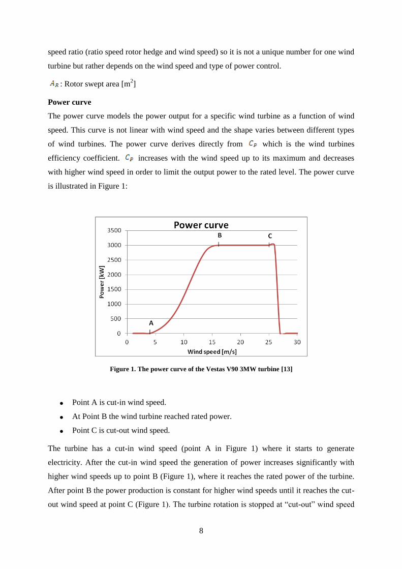
Power curve
The power curve models the power output for a specific wind turbine as a function of wind
speed. This curve is not linear with wind speed and the shape varies between different types
of wind turbines. The power curve derives directly from which is the wind turbines
efficiency coefficient. increases with the wind speed up to its maximum and decreases
with higher wind speed in order to limit the output power to the rated level. The power curve
is illustrated in Figure 1:
Figure 1. The power curve of the Vestas V90 3MW turbine [13]
Point A is cut-in wind speed.
At Point B the wind turbine reached rated power.
Point C is cut-out wind speed.
The turbine has a cut-in wind speed (point A in Figure 1) where it starts to generate
electricity. After the cut-in wind speed the generation of power increases significantly with
higher wind speeds up to point B (Figure 1), where it reaches the rated power of the turbine.
After point B the power production is constant for higher wind speeds until it reaches the cut-
out wind speed at point C (Figure 1). The turbine rotation is stopped at “cut-out” wind speed

9
because of safety reasons. In order to calculate the average power production of the wind
turbine, the product of the probability density function of the wind speed and the turbine´s
power curve are integrated [14], [15].
Wind Resources
By looking at equation 1 and 2 it can be determined that a small change in wind speed
contribute to a large change in power. A double in wind speed provides eight times the power
content. Because of this it is very important to evaluate the wind conditions at the site, when
planning a wind farm. At most sites worldwide the wind follows the Weibull- or the
simplified Rayleigh distribution. When using the Rayleigh distribution for modeling the
probability of the wind at a specific site, the only parameter which has to be known is the
average wind speed. The probability distribution, P( ), of the wind speed, , has the
following form:
Figure 2. Probability density function of a Rayleigh distribution with the mean speed 8 m/s
Production estimates
The wind forecasts and production estimates of a wind farm are very dependent of the
weather and it fluctuates over the seasons. Figure 3 below shows how the wind resources,
power curve and capacity factor are linked together by implementing them in the same graph.
As mentioned before, the average power production of the wind turbine is calculated by

10
integrating the product of the probability density function of the wind speed and the turbine´s
power curve. This is pictured in the graph as the relative energy extracted per wind speed.
Figure 3. The picture shows: the power curve of the Vestas V90 3MW turbine, the probability density
function of a Rayleigh distribution with the mean speed 8 m/s and the relative energy extracted per wind
speed.
The ability for a wind turbine to deliver energy over a selected period is called the capacity
factor . The capacity factor is defined as the ratio between the average power production
of the wind turbine and the rated power of the wind turbine. The equation below shows how
the capacity factor is calculated by dividing the expected energy production in a year with the
rated energy of the turbine.
2.1.2 Wind turbines
A wind turbine converts kinetic energy of the wind into mechanical energy and further into
electrical energy. The wind turbine captures the wind energy with the blades and converts the
wind power into mechanical rotational energy. The wind turbine can be equipped with
different number of blades and the amount depends on the location and application. Figure 4
shows a common setup of components included in a wind turbine.

11
Figure 4. Common setup of components included in a wind turbine. [19]
Blades
The rotational speed is limited by the number of blades and fast running rotors should have
few blades [16]. When generating electricity the generator need high speed at low torque. For
this reason most wind turbines used for this application are equipped with two or three blades.
Turbines with two blades has lower investment cost and the rotor speed is slightly higher than
the equivalent three bladed turbine. Two blades wind turbines are also subject to higher
mechanical forces variations on the drive train during one rotation. The motion of a three
bladed turbine is steadier and they are visually more accepted, the slightly lower speed also
contributes to less aerodynamic noise. As a consequence of, the three-bladed turbine has
become the norm, at least for onshore applications. For installations offshore the two bladed
versions might be considered in the future due to less investment cost, lighter weight and less
visual- and noisily impact on the public. The blades can be made of different materials and the
combination varies with turbine size. For larger wind turbines, like the 3 MW Vestas V90
turbine, fiber glass reinforced epoxy and carbon fibers, is used [13].
Power control

12
Stalling or pitching are two different ways of controlling the angle at which the wind strikes
the blades. This is called controlling the angle of attack and is used for limiting the power in
cases where the wind speed exceeds the rated limit of the turbine.
Stalling is a passive approach of controlling the angle of attack by aerodynamically designing
the blades. When the wind speed exceeds the rated limit, the angle of attack is increased and
some of the wind flow is replaced by turbulence which decreases the lifting force.
Pitch control is an active approach where an electronic controller senses the power output
from the turbine and directly pitches the blades out of the wind in case of unsafe wind speeds.
This approach provides a better control of the output power and all large modern turbines are
using pitch control [14], [15].
Gearbox
In order to increase the speed of the shaft and make the rotational speed suitable for the
generator, many turbines use a gearbox. A gearbox consists of many moving parts which are a
risk of failure. To reduce friction and mechanical losses, the moving parts in the gearbox are
embedded in oil. In the case where the turbines use a direct drive generator, capable of
producing electricity at low rotational speed, the gearbox can be excluded [14], [15].
Generators
A typical large wind turbine has either an induction- or synchronous generator for converting
the kinetic energy into electrical energy. Synchronous generators are until now quite rarely
used because of large size and the need for expensive minerals for the permanent magnets.
The benefit of a synchronous generator is that it can extract power from low rotational speeds
with high torque which makes it suitable for gearless wind turbines [14].
Power converter
Many wind turbines operate at variable speed in order to improve the performance of the wind
turbines. This is performed by keeping the tip speed ratio at a given wind speed as close to the
design tip speed ratio at which the efficiency of the turbine is optimized. As a result the
generator produces electricity with variable frequency. It is therefore necessary that power
electronics are used to match voltage- and frequency level to the one of the grid. The power
converter controls the current by using AC/DC and DC/AC converters which also make it
possible to control active- and reactive power up to certain limits. The rating of the power
electronics depends on the type of wind turbines; e.g. DFIG have only 30% rated power
electronics [15], [16].
13
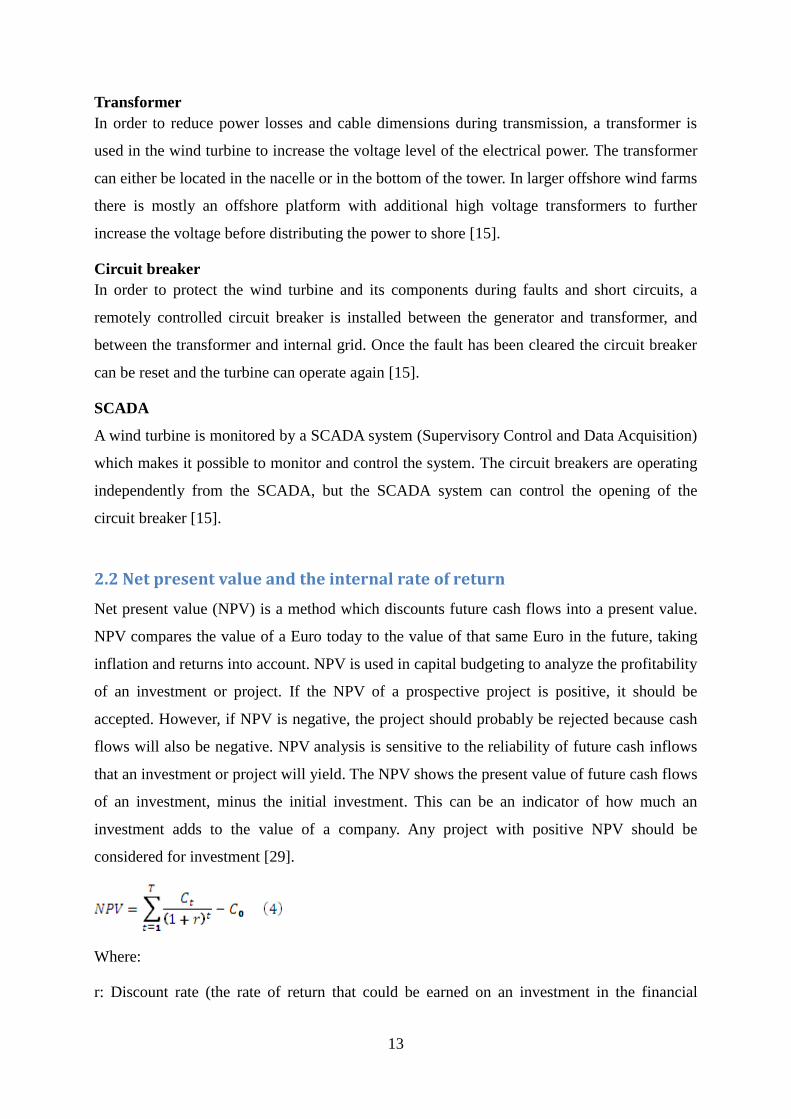
Transformer
In order to reduce power losses and cable dimensions during transmission, a transformer is
used in the wind turbine to increase the voltage level of the electrical power. The transformer
can either be located in the nacelle or in the bottom of the tower. In larger offshore wind farms
there is mostly an offshore platform with additional high voltage transformers to further
increase the voltage before distributing the power to shore [15].
Circuit breaker
In order to protect the wind turbine and its components during faults and short circuits, a
remotely controlled circuit breaker is installed between the generator and transformer, and
between the transformer and internal grid. Once the fault has been cleared the circuit breaker
can be reset and the turbine can operate again [15].
SCADA
A wind turbine is monitored by a SCADA system (Supervisory Control and Data Acquisition)
which makes it possible to monitor and control the system. The circuit breakers are operating
independently from the SCADA, but the SCADA system can control the opening of the
circuit breaker [15].
2.2 Net present value and the internal rate of return
Net present value (NPV) is a method which discounts future cash flows into a present value.
NPV compares the value of a Euro today to the value of that same Euro in the future, taking
inflation and returns into account. NPV is used in capital budgeting to analyze the profitability
of an investment or project. If the NPV of a prospective project is positive, it should be
accepted. However, if NPV is negative, the project should probably be rejected because cash
flows will also be negative. NPV analysis is sensitive to the reliability of future cash inflows
that an investment or project will yield. The NPV shows the present value of future cash flows
of an investment, minus the initial investment. This can be an indicator of how much an
investment adds to the value of a company. Any project with positive NPV should be
considered for investment [29].
Where:
r: Discount rate (the rate of return that could be earned on an investment in the financial

14
markets with similar risk also known as Weighted Average Cost of Capital - WACC)
T: Time of the cash flow
: Net cash flow (the amount of cash, inflow minus outflow) at the end of year t
: Initial investment cash outlay
The internal rate of return (IRR) is the discount rate that results in a net present value of zero
for a series of future cash flows. IRR is just like NPV an approach to evaluate whether an
investment is beneficial or not. The difference between the IRR and NPV is that IRR is the
true interest yield expected from an investment expressed as a percentage while the NPV is
expressed in monetary units like for example Euro´s. When comparing different investment
alternatives the project with the highest IRR should be chosen [29].
2.3 Power system reliability
Reliability is a term which is generally referred to the ability of a system or component to
perform in intended manner [1]. In a power system, reliability referrers to the ability of the
system to satisfy the load demand. The reliability assessment of a power system can be
divided into two main aspects which are system adequacy and system security.
Figure 5. Subdivision of system reliability [2]
The system adequacy evaluates whether there are sufficient facilities within the system in
order to fulfill the system operational constraints and load demand of the consumer. The
considered facilities related to system adequacy are everything from generating required
amount of energy in order to satisfy the consumer, to transmission and distribution facilities
15
needed for transporting the energy to the load point. One can say that adequacy is associated
with static conditions [1], [2].
System security considers the system ability of responding to dynamic or transient
disturbances arising within the system. These disturbances include local and widespread
failures along with abrupt losses of generation or transmission facilities. Combined or alone
these disturbances can lead to dynamic, transient or voltage instability of the system.
For the overall system function these two concepts are dependent of each other but in terms of
reliability evaluation they are treated separately and the evaluation is conducted in only one of
the domains. In most cases, along with this report, the focus lays on system adequacy for
conducting reliability analysis in power systems.
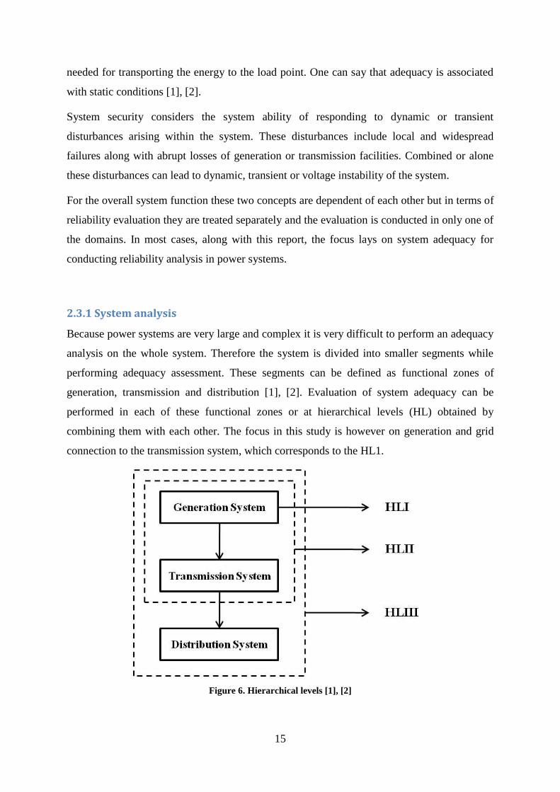
2.3.1 System analysis
Because power systems are very large and complex it is very difficult to perform an adequacy
analysis on the whole system. Therefore the system is divided into smaller segments while
performing adequacy assessment. These segments can be defined as functional zones of
generation, transmission and distribution [1], [2]. Evaluation of system adequacy can be
performed in each of these functional zones or at hierarchical levels (HL) obtained by
combining them with each other. The focus in this study is however on generation and grid
connection to the transmission system, which corresponds to the HL1.
Figure 6. Hierarchical levels [1], [2]

16
2.3.2 Analytical methods and Monte Carlo simulation
Power system reliability evaluation can be performed using analytical methods or Monte
Carlo simulation, where the results, in both cases, are numerical parameters in form of
reliability indices. These indices represent the capability of the system to provide the
customers by acceptable level of supply. Analytical techniques represent the system by
mathematical models and evaluate the reliability indices from these models using numerical
solutions. The Monte Carlo simulation estimates the reliability indices by simulating the
actual process and random behavior of the system. This method is more flexible and precise
than the analytical technique but it is more computational intensive [5]. In this work,
NEPLAN software was used which implements an analytical method.
2.3.3 Reliability indices
In order to perform a reliability assessment a first step is to transform the physical system to
an appropriate and simple model. This system model can e.g. be generated by using the
stochastic and memory less Markov process. In this process the present state of the system
depends on the immediately preceding event but is independent of all former states.
Figure 7. Markov two state model for one unit [1]
The basic two-state reliability model for a power system component is shown in Figure 7 and
the state of the unit can be either in- or out of service. The state of the system can be pictured
as a binary process. The probabilistic failure frequency for a certain unit is called failure rate
and is denoted [1/year] and the outage time for a unit in its failure state is denoted
[hour/failure] [1].
By multiplying the failure rate with the outage time and dividing them with the number
of hours per year, we get the total unavailability per year in percent for one component.
17
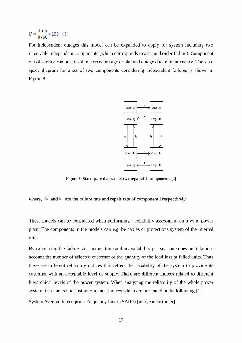
For independent outages this model can be expanded to apply for system including two
repairable independent components (which corresponds to a second order failure). Component
out of service can be a result of forced outage or planned outage due to maintenance. The state
space diagram for a set of two components considering independent failures is shown in
Figure 8.
Figure 8. State space diagram of two repairable components [4]
where, and are the failure rate and repair rate of component i respectively.
These models can be considered when performing a reliability assessment on a wind power
plant. The components in the models can e.g. be cables or protections system of the internal
grid.
By calculating the failure rate, outage time and unavailability per year one does not take into
account the number of affected customer or the quantity of the load loss at failed units. Thus
there are different reliability indices that reflect the capability of the system to provide its
customer with an acceptable level of supply. There are different indices related to different
hierarchical levels of the power system. When analyzing the reliability of the whole power
system, there are some customer related indices which are presented in the following [1].
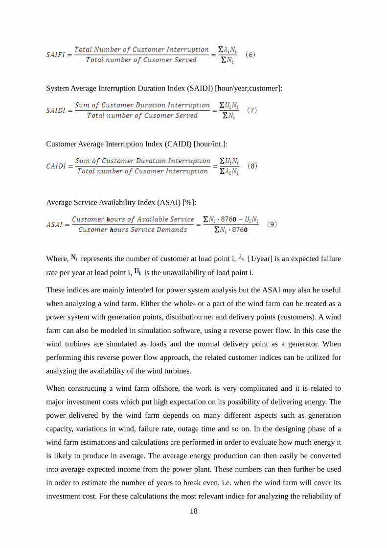
System Average Interruption Frequency Index (SAIFI) [int./year,customer]:
18
System Average Interruption Duration Index (SAIDI) [hour/year,customer]:
Customer Average Interruption Index (CAIDI) [hour/int.]:
Average Service Availability Index (ASAI) [%]:
Where, represents the number of customer at load point i, [1/year] is an expected failure
rate per year at load point i, is the unavailability of load point i.
These indices are mainly intended for power system analysis but the ASAI may also be useful
when analyzing a wind farm. Either the whole- or a part of the wind farm can be treated as a
power system with generation points, distribution net and delivery points (customers). A wind
farm can also be modeled in simulation software, using a reverse power flow. In this case the
wind turbines are simulated as loads and the normal delivery point as a generator. When
performing this reverse power flow approach, the related customer indices can be utilized for
analyzing the availability of the wind turbines.
When constructing a wind farm offshore, the work is very complicated and it is related to
major investment costs which put high expectation on its possibility of delivering energy. The
power delivered by the wind farm depends on many different aspects such as generation
capacity, variations in wind, failure rate, outage time and so on. In the designing phase of a
wind farm estimations and calculations are performed in order to evaluate how much energy it
is likely to produce in average. The average energy production can then easily be converted
into average expected income from the power plant. These numbers can then further be used
in order to estimate the number of years to break even, i.e. when the wind farm will cover its
investment cost. For these calculations the most relevant indice for analyzing the reliability of
19
the system is Energy Not Supplied (ENS) [MWh/year]. ENS is affected by both failure rate
and outage time which reflects the reliability of a wind farm. The ENS-value is suitable in
order to evaluate how much of the expected energy that will not be produced and supplied to
the customers. It is also useful in comparing the benefits of reliability improvements in
different wind farm topologies. The difference in the ENS-index can also be converted into
economical benefits achieved by reliability improvements.
Energy Not Supplied (ENS) [MWh/year]:
where is average load in MW connected to load point i and is the unavailability of
load point i.
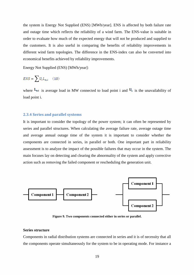
2.3.4 Series and parallel systems
It is important to consider the topology of the power system; it can often be represented by
series and parallel structures. When calculating the average failure rate, average outage time
and average annual outage time of the system it is important to consider whether the
components are connected in series, in parallel or both. One important part in reliability
assessment is to analyze the impact of the possible failures that may occur in the system. The
main focuses lay on detecting and clearing the abnormality of the system and apply corrective
action such as removing the failed component or rescheduling the generation unit.
Figure 9. Two components connected either in series or parallel.
Series structure
Components in radial distribution systems are connected in series and it is of necessity that all
the components operate simultaneously for the system to be in operating mode. For instance a
20
system with two series components requires functioning of both components in order to be
available. For a radial distribution system, which is comparable to a collection grid of an
offshore wind park, with i number of series components supplying load s, the related
equations are defined in the following [6].
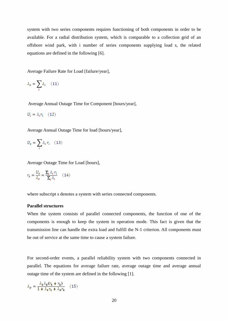
Average Failure Rate for Load [failure/year],
Average Annual Outage Time for Component [hours/year],
Average Annual Outage Time for load [hours/year],
Average Outage Time for Load [hours],
where subscript s denotes a system with series connected components.
Parallel structures
When the system consists of parallel connected components, the function of one of the
components is enough to keep the system in operation mode. This fact is given that the
transmission line can handle the extra load and fulfill the N-1 criterion. All components must
be out of service at the same time to cause a system failure.
For second-order events, a parallel reliability system with two components connected in
parallel. The equations for average failure rate, average outage time and average annual
outage time of the system are defined in the following [1].

21
where subscript p denotes a system with parallel connected components.

22
CHAPTER 3: NEPLAN
NEPLAN is a software which will be used in this project in order to evaluate different
topologies of a wind farm. The software is suitable for this purpose as it can handle reliability
calculations with the load considering constraints on the cable capacity.
3.1 NEPLAN Planning and Optimization Software
NEPLAN is planning and optimization software for electrical, heat, gas and water networks
which has been developed by the BCP group in Switzerland. It is used to analyze, plan,
optimize and manage power networks which includes optimal power flow, transient stability
and reliability analysis. The software package can be used for transmission and distribution
system analysis and the reliability software can provide reliability indices for individual load
points and the overall power system. It can also provide information based on the cost of
unreliability along with investment analysis and the Net Present Value (NPV) of different
investment alternatives. NEPLAN uses the homogenous Markov process for the calculations
and it handles up to second order contingencies. The NEPLAN tool is very flexible and user
friendly planning tool where network designers can compile different topologies. [3], [4].
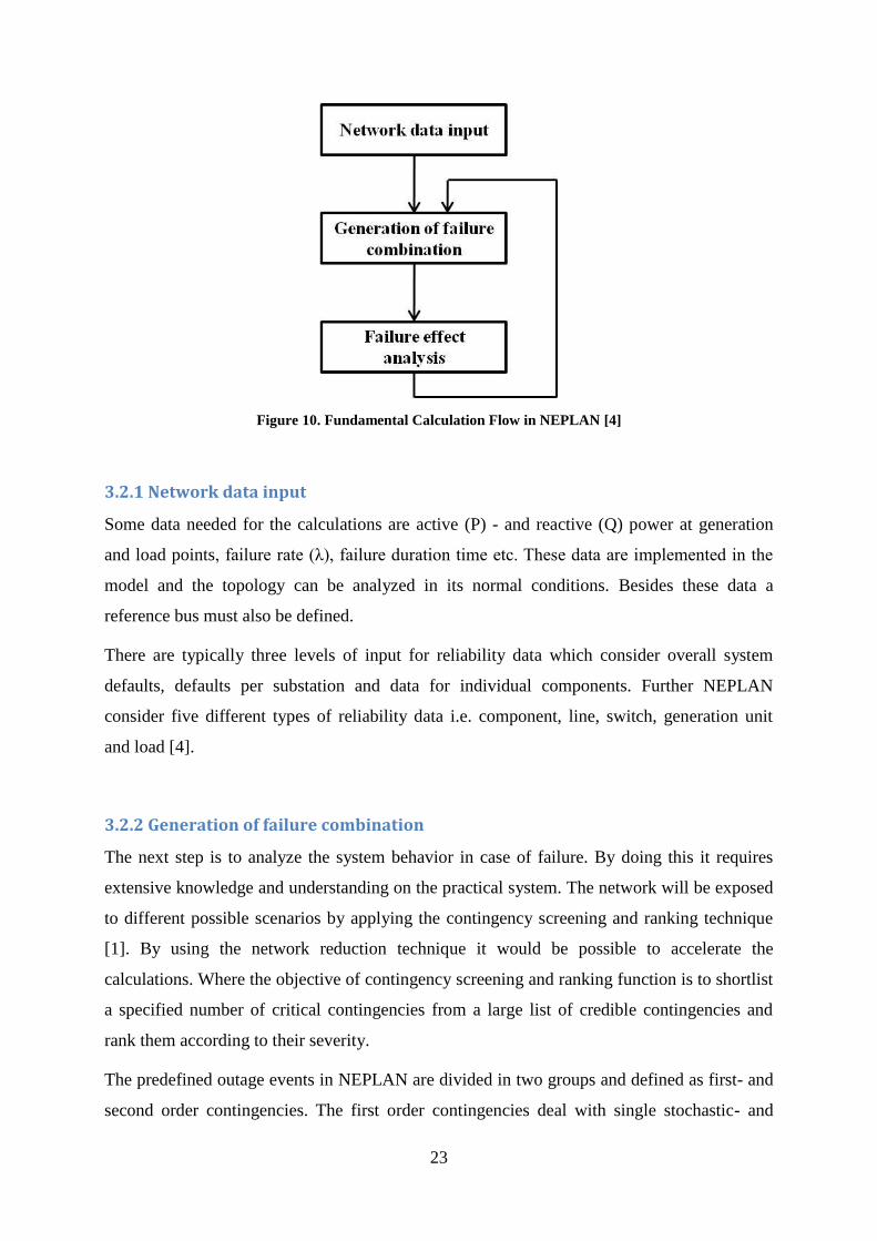
3.2 Fundamental Calculation Flow in NEPLAN
NEPLAN as a reliability analysis tool is based on the Markov method which is briefly
explained in previous chapter. The fundamental calculation flow in NEPLAN can be
visualized as in figure 6. The output of this evaluation approach is reliability indices for both
load point and the overall system along with load flow constraints [4].
23
Figure 10. Fundamental Calculation Flow in NEPLAN [4]
3.2.1 Network data input
Some data needed for the calculations are active (P) - and reactive (Q) power at generation
and load points, failure rate (λ), failure duration time etc. These data are implemented in the
model and the topology can be analyzed in its normal conditions. Besides these data a
reference bus must also be defined.
There are typically three levels of input for reliability data which consider overall system
defaults, defaults per substation and data for individual components. Further NEPLAN
consider five different types of reliability data i.e. component, line, switch, generation unit
and load [4].
3.2.2 Generation of failure combination
The next step is to analyze the system behavior in case of failure. By doing this it requires
extensive knowledge and understanding on the practical system. The network will be exposed
to different possible scenarios by applying the contingency screening and ranking technique
[1]. By using the network reduction technique it would be possible to accelerate the
calculations. Where the objective of contingency screening and ranking function is to shortlist
a specified number of critical contingencies from a large list of credible contingencies and
rank them according to their severity.
The predefined outage events in NEPLAN are divided in two groups and defined as first- and
second order contingencies. The first order contingencies deal with single stochastic- and

24
single deterministic outages while the second order contingencies can be considered either as
two stochastic- or stochastic and deterministic outages.
The different failure combinations can consist of single stochastic outages, overlap of two
stochastic outages or overlap of one stochastic and one deterministic outage.
Single stochastic outages can consist of single independent- or common mode outage, ground
fault or unintended switch opening. The reliability input data for these categories are failure
rate and repair time, the output data are failure frequency and its relevant duration.
Second order contingencies can be considered either as two stochastic outages or stochastic
and deterministic outages.
3.2.3 Overlapping stochastic outages
Independent outages can occur at the same time and overlap one and another. They are then
called overlapping stochastic outages and can consist of numerous different combinations like
[4]:
multiple independent failures
single independent failure plus manual disconnection
single independent failure plus common mode failure
single independent failure plus line-to-ground fault
multiple manual disconnections
manual disconnection plus common mode failure
manual disconnection plus line-to-ground fault
multiple common mode failures
common mode failure plus line-to-ground fault

25
The occurrence of overlapping outages can be graphically visualized as in Figure 11.
Figure 11. Overlapping stochastic outages [4]
In the case of overlapping of two stochastic outages, named A and B, the failure frequency
can be obtained from the homogenous Markov process [1].
where and are the failure rate and is their relevant repair time.
In the case where the second outage is a consequence of the first one, they are said to be
dependent and the second outage may occur with the probability Pr. This can be the case with
multiple ground faults due to increased voltage during the first, which may lead to second
short circuit. Another case is when protection fail to trip or trip unwanted due to faulty
protection settings. For dependent outages the failure frequency can be calculated as [1].
Deterministic outage, like preventive maintenance, do by itself not cause load supply
interruptions in the system. When though deterministic and stochastic outages occur at the
same time it may lead to forced outage and load failure. The processing of such overlapping
outages proceeds in the same way as single stochastic outages. The failure frequency at load
points can be calculated as [1].
where and are the failure rate for stochastic and deterministic outages respectively and
is their relevant repair time for maintenance.

26
3.2.4 Failure effect analysis
The final step includes evaluation of the effect contributed by possible failure outcomes. All
the possible failures are registered and the relevant indices associated to each load points and
the overall network is calculated. In this step the effects of load flow and the need for load
shedding is also presented by NEPLAN. The reliability indices which are provided by
NEPLAN is shown in Table 1 for individual load points and in
Table 2 for the overall power system.
Table 1. Load point indices [4], [5]
Index Unit Description
Interruption Frequency [1 /yr] Expected frequency of supply interruption per year
Interruption Duration [min/ yr]
[hrs/ yr]
Expected probability of interruption in minute or hours per year
Mean Time of interruption [min,hrs] Average duration of customer interruption
Power not supplied [kW/ yr]
[MW/ yr]
Product of interrupted power and its interruption frequency
Energy not supplied [kWh/ yr]
[MWh/ yr]
Product of interrupted power and its interruption probability
Interrupted cost [$/ yr] Cost of supply interruption
Table 2. Overall system indices [4], [5]
Index Unit Description
N - Total number of customers served
SAIFI [1/ yr] System average interruption
frequency index
SAIDI [min/yr] System average interruption index
CAIDI [h] Customer average interruption
duration index
ASAI [%] System average availability index
F [1/ yr] System load interruption frequency
T [h] System load interruption frequency
Q [min/ yr] System load interruption probability
P [MW/ yr] Total interrupted load power
W (ENS) [MWh/ yr] Total load energy not supplied
C [CU/ yr] Total load interruption cost
27
3.3 Example cases with NEPLAN and analytical calculations without
considering load flow
The aim of this section is to provide basic understanding of how NEPLAN executes its
calculations. This is carried out by; Building a simple network model in NEPLAN and apply
manual hand calculations in order to obtain load point indices and clarify the reliability
calculation approach. The objective is also to demonstrate how the software calculates the
indices. Calculations will be performed on series- and combined series and parallel networks.
This procedure is suitable while working with complex systems like a wind power system. In
order to execute a proper analysis of such systems a certain level of modeling has to be made.
When modeling a complicated system, a good approach is to divide the system into smaller
parts such as subsystems or components.
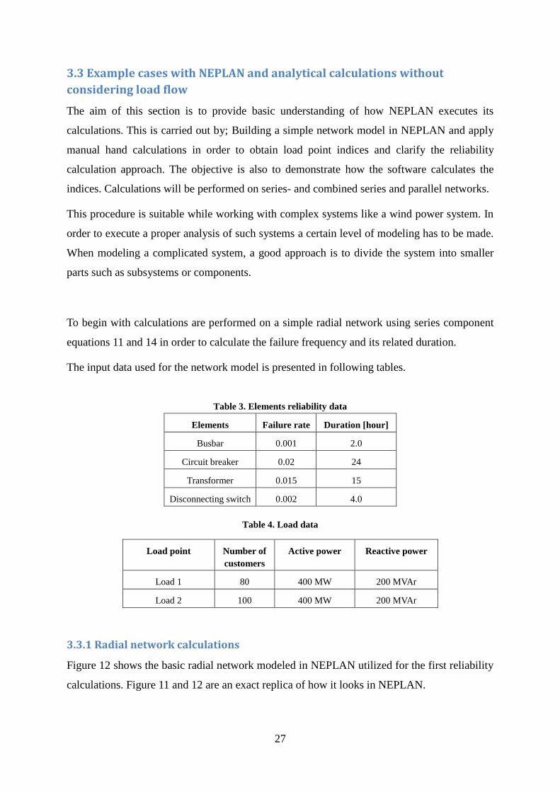
To begin with calculations are performed on a simple radial network using series component
equations 11 and 14 in order to calculate the failure frequency and its related duration.
The input data used for the network model is presented in following tables.
Table 3. Elements reliability data
Elements Failure rate Duration [hour]
Busbar 0.001 2.0
Circuit breaker 0.02 24
Transformer 0.015 15
Disconnecting switch 0.002 4.0
Table 4. Load data
Load point Number of
customers
Active power Reactive power
Load 1 80 400 MW 200 MVAr
Load 2 100 400 MW 200 MVAr
3.3.1 Radial network calculations
Figure 12 shows the basic radial network modeled in NEPLAN utilized for the first reliability
calculations. Figure 11 and 12 are an exact replica of how it looks in NEPLAN.

28
Figure 12. Radial network
Hand calculation of Load point indices for Load 1:
Failure duration calculation for load point 1:
System indices are calculated for load point 1, using equations 6-9:
29
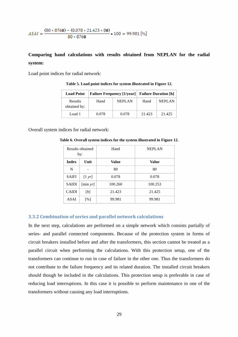
Comparing hand calculations with results obtained from NEPLAN for the radial
system:
Load point indices for radial network:
Table 5. Load point indices for system illustrated in Figure 12.
Load Point Failure Frequency [1/year] Failure Duration [h]
Results
obtained by:
Hand NEPLAN Hand NEPLAN
Load 1 0.078 0.078 21.423 21.425
Overall system indices for radial network:
Table 6. Overall system indices for the system illustrated in Figure 12.
Results obtained
by:
Hand NEPLAN
Index Unit Value Value
N - 80 80
SAIFI [1 yr] 0.078 0.078
SAIDI [min yr] 100.260 100.253
CAIDI [h] 21.423 21.425
ASAI [%] 99.981 99.981
3.3.2 Combination of series and parallel network calculations
In the next step, calculations are performed on a simple network which consists partially of
series- and parallel connected components. Because of the protection system in forms of
circuit breakers installed before and after the transformers, this section cannot be treated as a
parallel circuit when performing the calculations. With this protection setup, one of the
transformers can continue to run in case of failure in the other one. Thus the transformers do
not contribute to the failure frequency and its related duration. The installed circuit breakers
should though be included in the calculations. This protection setup is preferable in case of
reducing load interruptions. In this case it is possible to perform maintenance in one of the
transformers without causing any load interruptions.

30
Figure 13 shows the combination of series and parallel network which is utilized for the
second reliability calculations.
Figure 13. Combination of series and parallel network
System indices are calculated for load point 2, using equations 6-9:

31
Comparing hand calculations with results obtained from NEPLAN for combined
network:
Load point indices for the combination of series and parallel network:
Table 7. Load point indices for system illustrated in Figure 13.
Load Point Failure Frequency [1/year] Failure Duration [h]
Results by: Hand NEPLAN Hand NEPLAN
Load 2 0.103 0.103 23.359 23.362
Overall system indices for the combination of series and parallel network:
Table 8. Overall system indices for the system illustrated in Figure 13.
Results by: Hand NEPLAN
Index Unit Value Value
N - 100 100
SAIFI [1/yr] 0.103 0.103
SAIDI [min/yr] 144.359 144.344
CAIDI h 23.359 23.362
ASAI % 99.973 99.973

32
CHAPTER 4: Offshore wind farm grid topology
The aim of this chapter is to illustrate the current state of the art in grid configuration of
offshore wind farms.
4.1 Different layouts for offshore collector systems/Common grid topology
structures
There are different arrangements for wind farm collector systems and the grid can be designed
for AC, DC or booth AC and DC. The study performed in this report does however only
consider AC transmission with a collector voltage of 33 kV. Cables are buried at a depth of
1,5-2m under the seabed to protect the cables from external damages. These conditions makes
that repair of cables can be difficult and long, especially if cable vessels necessary to the
work, are not available.
Most operational offshore wind farms have radial internal array grid connection topologies.
An exception is North Hoyle [17] and some more recent projects, such as the Alpha Ventus
[27] and Great Gabbard [28] which also includes redundancy. This may suggest that electrical
grid designer have identified these topologies advantageous. The radial topology has however
been reconsidered for upcoming wind farms and including redundancy, like North Hoyle, has
become a topic. Alternative designs and possible future designs are discussed in the following
sections.
The electrical system for an offshore wind farm concerns all those components that enable the
integration of the wind turbine to the grid supply point. Examples of such components are
generating units, switchgear, transformers, inter turbines and transmission cables, power
electronic converters etcetera. The overall function of the electrical system is to collect power
from each wind turbines, to transmit the power to shore and to convert it to appropriate grid
voltage and frequency. When designing the overall wind farm the aim is to minimize the
energy cost by balancing the overall wind production, (- taking into account the distribution of
wind speed and direction as well as the turbulence between turbines (wake effect), bathymetry
and geotechnical conditions), and investment and operational costs.

33
There have been several studies performed in evaluating different layouts for offshore
collector systems. There is a project called Downvind (Distant Offshore Wind farms with No
Visual Impact in Deepwater) where a project group studied and evaluated the offshore grid of
offshore wind farms. In this study, four different conceptual designs have been identified [18]:
Radial design, where all wind turbines are connected to a single cable feeder within a
string.
Single-sided ring design, where a redundant path is included for the power flow within
a string.
Double-sided ring design, where redundancy is provided by the establishment of a
looped circuit between the wind turbines.
Star design, where the wind turbines are distributed over several feeders, allowing the
use of lower rated equipment.
The options may all be utilized for both AC and DC solutions. These four design options are
presented in the following along with two additional alternatives.
4.1.1 Radial design
Figure 14 shows the layout of a radial offshore grid where the wind turbines are connected to
a single cable feeder within a string and collected at the collector hub. The maximum number
of wind turbines that can be connected to each string feeder is determined by the subsea cable
ratings and the capacity of the generator. This design is simple to control but the main
advantage is the relatively low cable costs due to the possibility of taper the cable ratings
between the turbines. This is possible because with increased distance from the hub and
decreasing numbers of turbines connected in series, the amount of power transmitted is
smaller further out in each feeder. The major disadvantage with this design is the
comparatively poor reliability. Cable or switchgear faults at the hub side of the feeder will
lead to the loss of power from all downstream turbines in the feeder [18], [14].

34
Figure 14. Radial design with one and two feeder cables to shore
4.1.2 Single-sided ring and shared ring design
Figure 15 shows the single-sided ring design. This design has additional parallel cables for
each string, forming a looped design. Comparing to the radial design this alternative addresses
some of the reliability issues by providing a redundant path for the power flow within a string.
In the single-sided ring design, this additional security comes at the expense of higher cable
costs due to the extra cable. This cable is installed from the collector hub to the last turbine in
the string with the switching device normally opened. This implies that in case of at fault
between the collector hub and the first turbine, it is not possible to taper the cable ratings
because the ringed path must be able to carry the entire power flow of all turbines. Despite the
increase in cable costs compared to the radial system, an initial feasibility commissioned by
the DOWNVInD consortium recommended and utilized this design for the studied 1 GW
offshore wind [18], [14].
Figure 15. Single sided ring design
4.1.3 Double-sided ring
Figure 16 shows the double sided ring, which is another version of a looped design. Two
strings are connected in parallel in order to provide redundancy. For this design solution the

35
cable length for the two strings will only increase by the distance between the turbines at the
end of the strings. Like for the single-sided ring design tapering of the cable ratings is maybe
not an alternative because all cables should be able to handle the full power flow of the extra
transmission in one string in case of fault. The cables ratings can be tapered and load shedding
can be performed in case of overload. This is however an economical issue, where the extra
installation costs must be weighed against the expected value of lost load over the lifetime of
the wind farm [18], [14].
Figure 16. Double-sided ring
4.1.4 Star design
Figure 17 shows the star design. In this design the cable ratings can be low and it can provide
a high level of security for the wind farm as a whole. In case of a cable outage, this will only
affect one wind turbine, except for the case when a fault occurs in the feeder cable to the hub.
Another advantage for this design is that the voltage regulation along the cables is likely to be
better. The downside for the star design is the increased expenses due to the longer diagonal
cable runs and the short section of the higher rated connection to the hub. The major cost
implication of this option is the more complex switchgear requirement at the central turbine of
the star [18], [14]Error! Reference source not found..
Figure 17. Star- or cluster design

36
4.1.5 Single return- or shared ring design
Figure 18 shows the design option single return- or shared ring design. This design consists of
a number of strings connected in parallel with a redundant cable. The redundant circuit is
designed to potentially deliver the full power output of a failing string within the arrangement.
The probability of two or more feeders failing at the same time is considered to be relatively
small and the redundant cable is dimensioned handle the load of one string only.
Figure 18. Single return- or shared ring design
4.1.6 Double-sided half-ring design
Figure 19 shows the double sided half-ring design which is a semi variant of the double sided
ring design. This is a configuration which could be interesting in case when little
modifications are coveted compared to the radial design. This layout can isolate five turbines
in case of a cable failure in the beginning of an array and provide an extra path for the
remaining five turbines. This layout should also include remote controlled load switches
booth in each array and the loop. In this way it is possible to remotely isolate five turbines at
the time.
Figure 19. Double-sided half-ring design

37
4.2 Thanet offshore wind farm
In this section the grid topology of the Thanet offshore wind farm is presented for illustration,
and as a basis for creating a topology base case. The 300 MW wind farm is currently the
largest offshore wind farm operating and it has been selected for this reason as representative
of the current state of the art in grid topology.
4.2.1 Basic information and location
The Thanet Offshore Wind Farm is owned by Vattenfall and the construction of the wind farm
was commissioned in September 2010. The total investment for completing the wind farm is
in the order of around £780 million. The wind farm consists of 100 Vestas V90 3 MW
turbines which gives a total capacity of 300 MW. The wind farm covers an area of 35 square
kilometers and is located approximately 12 kilometers north east of Foreness Point, the
eastern tip of Kent. The onshore power substation is located in Richborough [20], [21].
Figure 20. Location of the Thanet offshore wind farm. [22]
Each wind turbine sits atop a steel monopole foundation at a water depth between 20 and 25
meters. The tower of the wind turbines is connected to the foundation by a transition piece.
The hub of the wind turbine is located at 70 m height above sea level. The wind farm consists
of seven rows where the distance between turbines is approximately 500 meters along the
rows and 800 meters between the rows. The inter-array cables interconnect the wind turbines
within the arrays to each other and to the offshore transformer substations. The cables are
standard 3-core, copper conductor, cross-linked polyethylene (XLPE) insulated and armoured
submarine cable, rated at 33 kV.
38
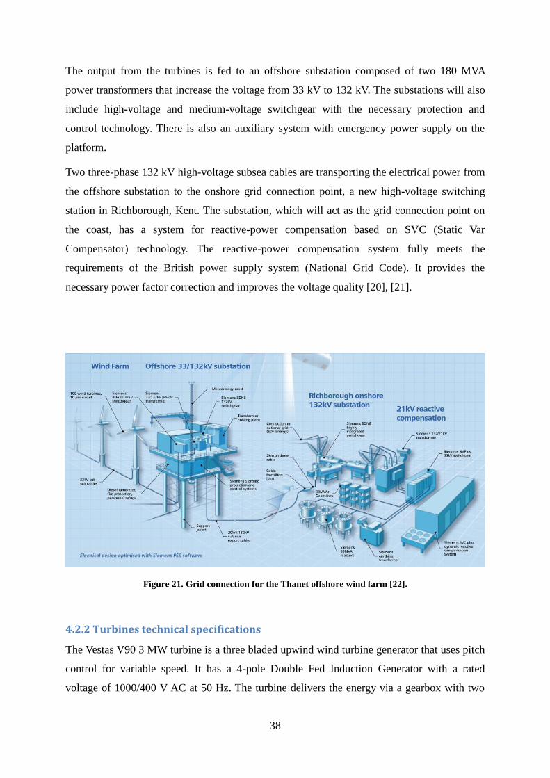
The output from the turbines is fed to an offshore substation composed of two 180 MVA
power transformers that increase the voltage from 33 kV to 132 kV. The substations will also
include high-voltage and medium-voltage switchgear with the necessary protection and
control technology. There is also an auxiliary system with emergency power supply on the
platform.
Two three-phase 132 kV high-voltage subsea cables are transporting the electrical power from
the offshore substation to the onshore grid connection point, a new high-voltage switching
station in Richborough, Kent. The substation, which will act as the grid connection point on
the coast, has a system for reactive-power compensation based on SVC (Static Var
Compensator) technology. The reactive-power compensation system fully meets the
requirements of the British power supply system (National Grid Code). It provides the
necessary power factor correction and improves the voltage quality [20], [21].
Figure 21. Grid connection for the Thanet offshore wind farm [22].
4.2.2 Turbines technical specifications
The Vestas V90 3 MW turbine is a three bladed upwind wind turbine generator that uses pitch
control for variable speed. It has a 4-pole Double Fed Induction Generator with a rated
voltage of 1000/400 V AC at 50 Hz. The turbine delivers the energy via a gearbox with two
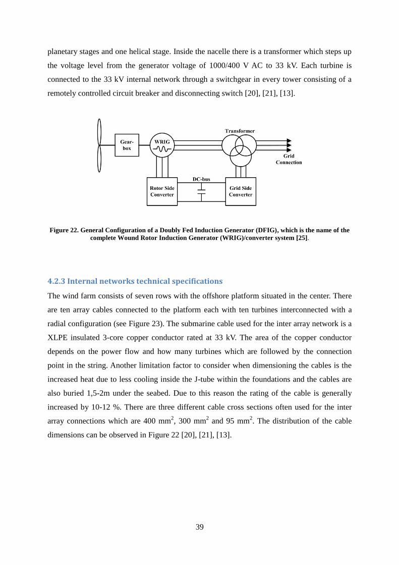
39
planetary stages and one helical stage. Inside the nacelle there is a transformer which steps up
the voltage level from the generator voltage of 1000/400 V AC to 33 kV. Each turbine is
connected to the 33 kV internal network through a switchgear in every tower consisting of a
remotely controlled circuit breaker and disconnecting switch [20], [21], [13].
Figure 22. General Configuration of a Doubly Fed Induction Generator (DFIG), which is the name of the
complete Wound Rotor Induction Generator (WRIG)/converter system [25].
4.2.3 Internal networks technical specifications
The wind farm consists of seven rows with the offshore platform situated in the center. There
are ten array cables connected to the platform each with ten turbines interconnected with a
radial configuration (see Figure 23). The submarine cable used for the inter array network is a
XLPE insulated 3-core copper conductor rated at 33 kV. The area of the copper conductor
depends on the power flow and how many turbines which are followed by the connection
point in the string. Another limitation factor to consider when dimensioning the cables is the
increased heat due to less cooling inside the J-tube within the foundations and the cables are
also buried 1,5-2m under the seabed. Due to this reason the rating of the cable is generally
increased by 10-12 %. There are three different cable cross sections often used for the inter
array connections which are 400 mm2, 300 mm
2 and 95 mm
2. The distribution of the cable
dimensions can be observed in Figure 22 [20], [21], [13].

40
Figure 23 – Layout of the Thanet wind farm. It is composed of ten array cables connecting one hundred 3
MW turbines to an offshore substation. At the substation, two 180 MVA transformers increase the voltage
from 33 kV to 132 kV. The electrical power is then transmitted to the onshore grid connection point in
Richborough by two three-phase 132 kV subsea cables [20].

41
CHAPTER 5: Analysis of different topologies
This chapter presents the data used for the models and the different topologies chosen for the
analysis are presented. Some drawbacks and benefits are also discussed for each topology.
The software NEPLAN is used in order to analyze power flow and reliability of different
topologies. For the study the distribution generators in the wind turbines are modeled and
represented as loads using a reverse power flow approach. The reason for this approach is to
be able to model the possibility to control the output power of the wind turbines, which was
not possible in NEPLAN for a generator. This is done for each load point (each wind turbine)
by allowing complete load (production) shedding. All the cables are modeled as pi-
equivalents in NEPLAN, working in steady state conditions. Parameters used for modeling
the cables, in addition to the reliability data, are: resistance R, inductance X, capacitance C
and the maximum current- and voltage ratings for the cable. The cable lengths and distances
between turbines and platform can be seen in Figure 24.
In the original topology along with the alternative topologies, there are different protections
elements like: circuit breakers, load switches and disconnectors included. These devices are
considered correctly dimensioned and treated as ideal elements during the load flow analysis.
For the reliability analysis, these elements are though of considerable importance because of
their contribution of the overall performance of the system. The reliability data used for
modeling are based on [6] and [10], with supplements from [26], and are presented in Table 9.
Table 9. Reliability data
Component Failure rate
[failure/year]
Repair time
[hours]
Switching time [min]
Subsea cables (33 kV) 0.004 672 -
Disconnectors (33 kV in wind turbines) (Manual) 0.01 120 10080*
Circuit breakers (33 kV on offshore platform) 0.03 120 20
Load switches (33 kV in wind turbines) 0.01 120 20
*One week switching time including isolation of the fault. Switching has to be performed by service
personal going to the turbine by boat.

42
When studying the different topologies and evaluating the change in performance on different
layouts, the only interesting parameters are: different cable ratings and reliability data for
cables and switching devices. Thus the wind turbines (bus and load) and the offshore platform
(bus and generator) are considered as ideal elements. For this study, voltage drop in the
system is neglected because this is considered rather easy to avoid and can be compensated
with reactive power in the reality. The cable loops which are included in some of the
topologies are modeled as ideal elements considering that faults occur rather seldom and that
the loops are not included in the regular performance of the network.
A wind farm is a very intermittent energy resource and the power production varies
considerably over time. Because of this it would not provide a fair comparison between the
different topology options if they only where modeled on maximum production level. In case
of failure the different topologies provides alternative paths for the power to flow, with
different power ratings. This fact contributes to different abilities of producing electricity
during fault compared to alternative layouts. In order to create a more realistic power
production scenario for each topology, the power production is divided in four different
production levels. Each level is based on the wind probability density function at the
production site, combined with the power curve of the Vestas V90 3 MW wind turbine. The
production level for each case is provided in Table 10.
Table 10. Production level for each case
Case Wind speed
[m/s]
Avg. production
[MW]
Probability
[%]
1 0-3 0 14
2 4-8 0,425 45
3 9-12 1,834 26,5
4 13-25 2,947 14,5
The average annual electricity generation in one year on the Thanet wind farm is 960 GWh.
[23] which corresponds to a capacity factor of 36,53%.
The ENS values for each case and topology are weighted with the probability for each case
and a mean value of ENS is presented in order to compare each topology. The calculations are
performed in Excel and only the ENS mean value is presented for each topology.

43
Cost data used in the study for investment analysis and evaluation whether a change in layout
could be financially beneficial or not, are collected from [10] and [24]. The data used for
investment analysis are presented in Table 11.
Table 11. Cost data used for investment analysis.
Discount rate 7 %
Expected income per MWh 0,18 [€/MWh]*
Expected lifetime of the wind farm 20 [years]
Vessel and installation cost, cable 200 [k€/km]
Load switch with V, I measurement 10 [k€]
Cable dimensions [mm2] Cost [k€/km]**
95 100
120 110
150 140
185 160
240 180
300 220
400 240
500 270
630 300
800 350
1000 360
1200 370
*Including electricity price and green certificates, valid 2010 in UK [24]. No predictions of future changes
and inflation rates are taken into account.
**Cable costs are collected from [10] for cable ratings up to 400 mm2 and an extrapolation of the costs is
performed for the remaining cable ratings.
Alternative layout, Top.1
Top.1 is the original topology of two branches on the Thanet wind farm which is used as a
benchmark for evaluation of different topologies. Each row consists of ten 3 MW turbines
with manual disconnectors situated in each tower and a voltage level of 33 kV. Each row of
turbines is terminated with a circuit breaker on the offshore platform which is pictured as a
bus to the left. The cables which are used to interconnect the turbines are three core armoured
33 kV XLPE copper cables.
In case of a fault on one of the cables the entire row is disconnected. The entire row with
turbines will be disconnected and not be able to produce any electricity until the fault is
identified and the affected cables and turbines are manually disconnected. This operation can
take rather long time depending on the prevailing weather conditions.

44
If a fault is located in one of the turbines, this turbine can be remotely disconnected with the
circuit breaker situated inside the turbine. In this way the remaining turbines can continue to
operate after the turbine which is out of order is disconnected.
Figure 24. Original layout, Top.1,
Alternative layout, Top.2
Top.2 is the first alternative layout which is analyzed. This layout is the same as the original
but a cable loop with a, normally open, remote controlled loadswitch is included in the end
which connect the two rows to eachother. A fault must be manually detected and isolated but
this alterntive can provide an extra path for the power to flow. In this layout the cables are
though not dimensioned to bear any extra load besides the ten turbines at full load. This
makes this layout not able to be fully utilized during strong winds and load shedding must be
performed in order to not overload the cables. Load shedding can be performed remotely by
turning the blades on the turbines. One should also consider that the average power
production is around 37 % of full load which makes this solution useful in normal
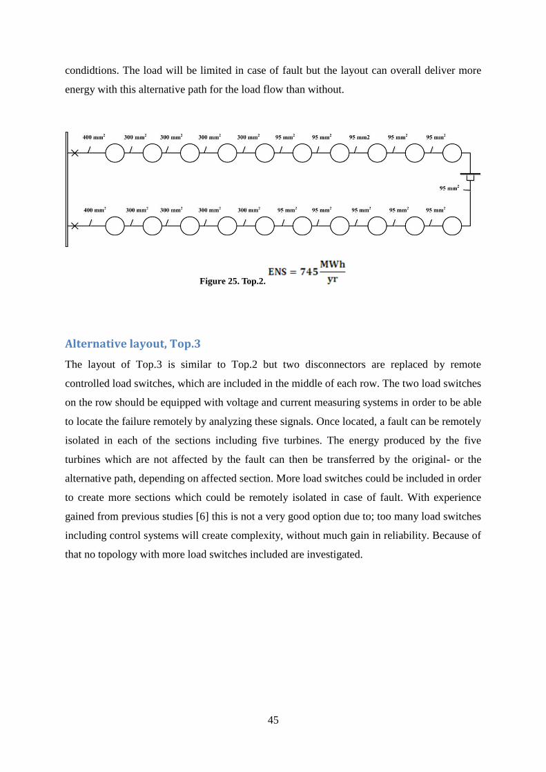
45
condidtions. The load will be limited in case of fault but the layout can overall deliver more
energy with this alternative path for the load flow than without.
Figure 25. Top.2.
Alternative layout, Top.3
The layout of Top.3 is similar to Top.2 but two disconnectors are replaced by remote
controlled load switches, which are included in the middle of each row. The two load switches
on the row should be equipped with voltage and current measuring systems in order to be able
to locate the failure remotely by analyzing these signals. Once located, a fault can be remotely
isolated in each of the sections including five turbines. The energy produced by the five
turbines which are not affected by the fault can then be transferred by the original- or the
alternative path, depending on affected section. More load switches could be included in order
to create more sections which could be remotely isolated in case of fault. With experience
gained from previous studies [6] this is not a very good option due to; too many load switches
including control systems will create complexity, without much gain in reliability. Because of
that no topology with more load switches included are investigated.
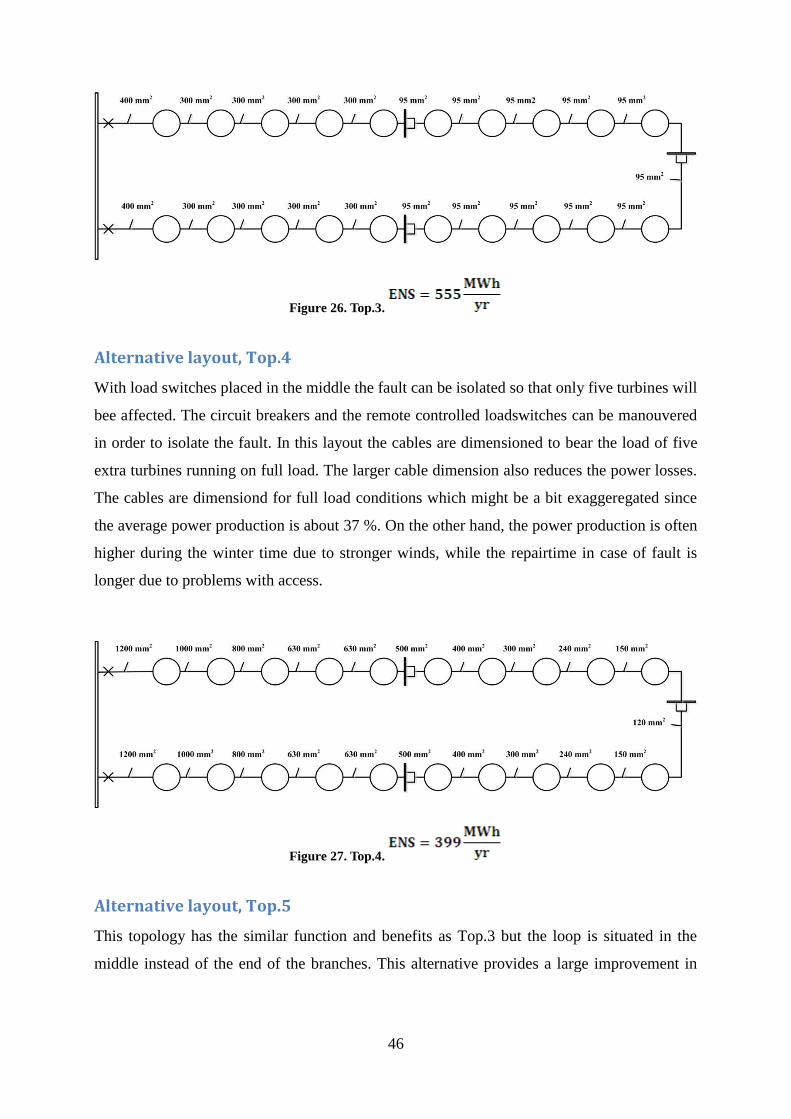
46
Figure 26. Top.3.
Alternative layout, Top.4
With load switches placed in the middle the fault can be isolated so that only five turbines will
bee affected. The circuit breakers and the remote controlled loadswitches can be manouvered
in order to isolate the fault. In this layout the cables are dimensioned to bear the load of five
extra turbines running on full load. The larger cable dimension also reduces the power losses.
The cables are dimensiond for full load conditions which might be a bit exaggeregated since
the average power production is about 37 %. On the other hand, the power production is often
higher during the winter time due to stronger winds, while the repairtime in case of fault is
longer due to problems with access.
Figure 27. Top.4.
Alternative layout, Top.5
This topology has the similar function and benefits as Top.3 but the loop is situated in the
middle instead of the end of the branches. This alternative provides a large improvement in
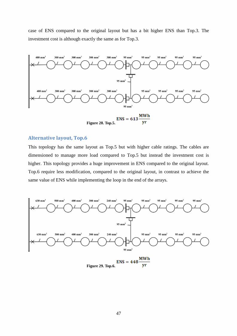
47
case of ENS compared to the original layout but has a bit higher ENS than Top.3. The
investment cost is although exactly the same as for Top.3.
Figure 28. Top.5.
Alternative layout, Top.6
This topology has the same layout as Top.5 but with higher cable ratings. The cables are
dimensioned to manage more load compared to Top.5 but instead the investment cost is
higher. This topology provides a huge improvement in ENS compared to the original layout.
Top.6 require less modification, compared to the original layout, in contrast to achieve the
same value of ENS while implementing the loop in the end of the arrays.
Figure 29. Top.6.
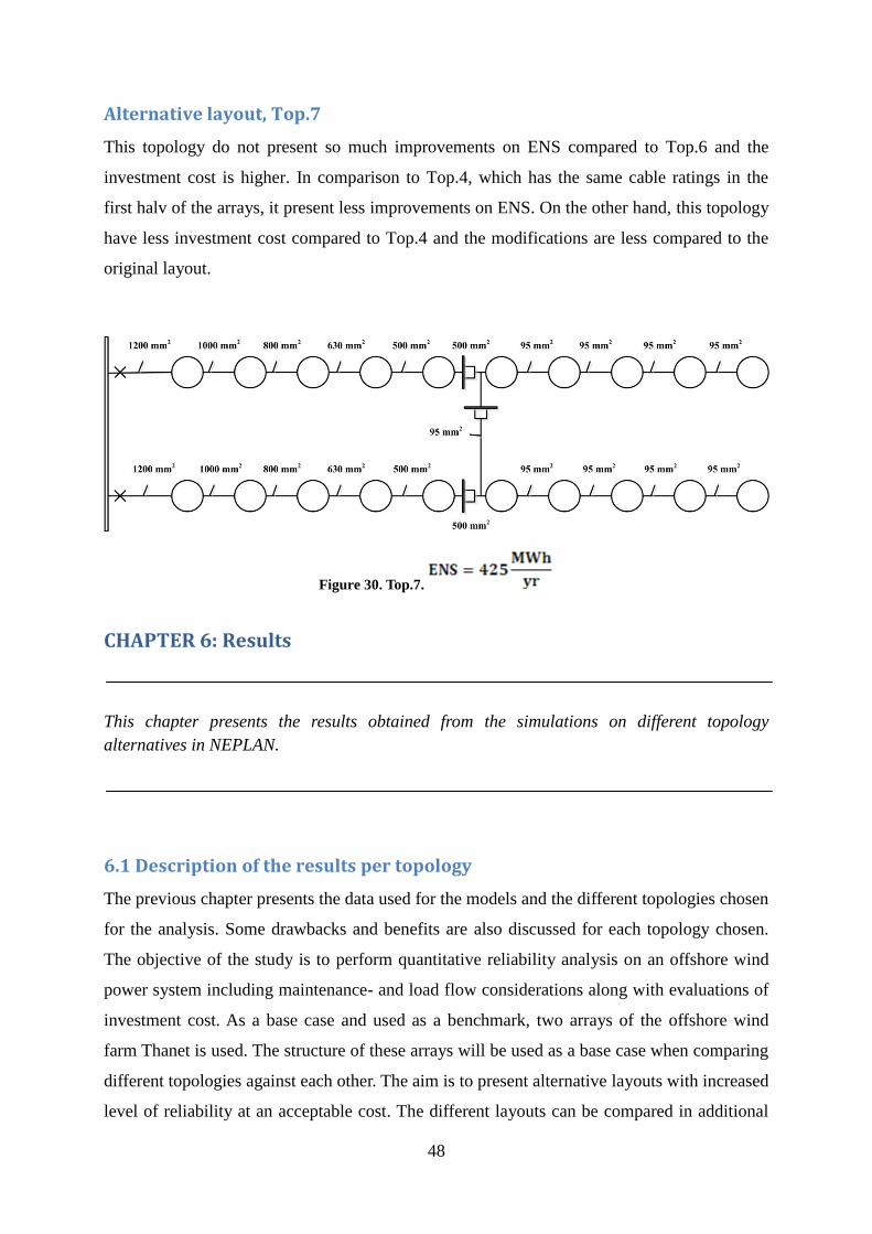
48
Alternative layout, Top.7
This topology do not present so much improvements on ENS compared to Top.6 and the
investment cost is higher. In comparison to Top.4, which has the same cable ratings in the
first halv of the arrays, it present less improvements on ENS. On the other hand, this topology
have less investment cost compared to Top.4 and the modifications are less compared to the
original layout.
Figure 30. Top.7.
CHAPTER 6: Results
This chapter presents the results obtained from the simulations on different topology
alternatives in NEPLAN.
6.1 Description of the results per topology
The previous chapter presents the data used for the models and the different topologies chosen
for the analysis. Some drawbacks and benefits are also discussed for each topology chosen.
The objective of the study is to perform quantitative reliability analysis on an offshore wind
power system including maintenance- and load flow considerations along with evaluations of
investment cost. As a base case and used as a benchmark, two arrays of the offshore wind
farm Thanet is used. The structure of these arrays will be used as a base case when comparing
different topologies against each other. The aim is to present alternative layouts with increased
level of reliability at an acceptable cost. The different layouts can be compared in additional

49
income over the life time of the wind farm, as the energy not supplied (ENS) is used in the
study. Seven different topologies are analyzed and compared with respect to the reliability of
the different designs. The seven different topologies with diverse level of redundancy are
based on various levels of investment costs. The Net Present Value and the Internal Rate of
Return are used for investment analysis. The different layouts also consist of different cable
ratings which contribute to various levels of power losses for each topology. The Average
System Availability Index (ASAI) [%] is presented for each case and it is of interest when
evaluating the level of load shedding needed for each topology showing the influence of cable
ratings. Figure 31visualizes the designation of each cable and Table 12 presents the influence
of each cable on the overall ENS.
Figure 31. Cable Layout
Different location and function of the cables contributes to different levels of ENS which is
visualized in Table 12 below.
Table 12. NEPLAN results and the influence of cables on ENS (case 4)
Top.1 Top.2 Top.3 Top.4 Top.5 Top.6 Top.7
Name Type F
[1/yr] T [h]
Q
[min/yr] ENS
[MWh/yr] ENS ENS ENS ENS ENS ENS
**Total** 0,481 170,663 4928,958 2154,533 2143,901 1726,048 1105,927 1999,947 1340,805 1183,595
1.1, 2.1 Cable 0,004 677,151 161,000 79,092 74,886 73,477 32,270 79,171 48,749 35,546
1.2, 2.2 Cable 0,002 679,525 80,427 36,530 34,369 33,670 13,076 36,512 21,313 14,714
1.3, 2.3 Cable 0,002 679,525 80,427 33,552 31,387 30,688 10,093 33,530 18,330 11,732
1.4, 2.4 Cable 0,002 679,525 80,427 30,575 28,404 27,706 7,111 30,546 15,348 8,751
1.5, 2.5 Cable 0,002 679,525 80,427 27,598 25,422 24,724 4,943 27,562 12,366 5,769
1.6, 2.6 Cable 0,002 679,525 80,427 24,621 22,440 17,658 4,905 19,808 8,277 4,911
1.7, 2.7 Cable 0,002 679,525 80,427 21,644 19,459 14,676 4,904 16,830 16,822 16,820
1.8, 2.8 Cable 0,002 679,525 80,427 18,668 16,477 11,695 4,903 13,854 13,843 13,841
1.9, 2.9 Cable 0,002 679,525 80,427 15,691 13,495 8,713 4,902 10,878 10,864 10,862
1.10, 2.10 Cable 0,002 679,525 80,427 12,715 10,514 5,732 4,902 7,902 7,886 7,883
Loop End* Cable - - - - 0 0 0 - - -
Loop
Middle*
Cable - - - - - - - 0 0 0
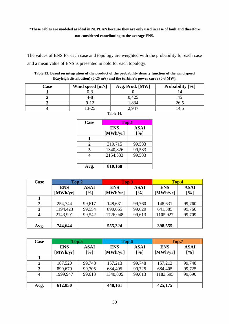
50
*These cables are modeled as ideal in NEPLAN because they are only used in case of fault and therefore
not considered contributing to the average ENS.
The values of ENS for each case and topology are weighted with the probability for each case
and a mean value of ENS is presented in bold for each topology.
Table 13. Based on integration of the product of the probability density function of the wind speed
(Rayleigh distribution) (0-25 m/s) and the turbine´s power curve (0-3 MW).
Case Wind speed [m/s] Avg. Prod. [MW] Probability [%]
1 0-3 0 14
2 4-8 0,425 45
3 9-12 1,834 26,5
4 13-25 2,947 14,5 Table 14.
Case Top.1
ENS
[MWh/yr]
ASAI
[%]
1
2 310,715 99,583
3 1340,826 99,583
4 2154,533 99,583
Avg. 810,168
Case Top.2 Top.3 Top.4
ENS
[MWh/yr]
ASAI
[%]
ENS
[MWh/yr]
ASAI
[%]
ENS
[MWh/yr]
ASAI
[%]
1
2 254,744 99,617 148,631 99,760 148,631 99,760
3 1194,423 99,554 890,665 99,620 641,385 99,760
4 2143,901 99,542 1726,048 99,613 1105,927 99,709
Avg. 744,644 555,324 398,555
Case Top.5 Top.6 Top.7
ENS
[MWh/yr]
ASAI
[%]
ENS
[MWh/yr]
ASAI
[%]
ENS
[MWh/yr]
ASAI
[%]
1
2 187,520 99,748 157,213 99,748 157,213 99,748
3 890,679 99,705 684,405 99,725 684,405 99,725
4 1999,947 99,613 1340,805 99,613 1183,595 99,690
Avg. 612,850 448,161 425,175

51
Table 15 shows the possible additional energy production and income for each topology. The
possible total extra income over the lifetime of 20 years is also calculated by multiplying the
additional income per year with 20 and then subtracting the additional investment for each
topology. These figures do not consider any fluctuations in electricity price, discount rate and
inflation rate.
Table 15. The additional annual energy that can be supplied for different topologies.
Wind farm
topology
Average ENS
[MWh/yr]
Add. Energy
that can be
supplied
[MWh/yr]
Add. Income
per year
[k€]
Add.
Investment
[k€]
Total Extra
income
(20 years)
[k€]
Top.1 810,168
Top.2 744,644 65,524 11,794 289,000 -53,113
Top.3 555,324 254,844 45,872 309,000 608,438
Top.4 398,555 411,613 74,090 1571,087 -89,280
Top.5 612,850 197,319 35,517 309,000 401,347
Top.6 448,161 362,007 65,161 474,848 828,379
Top.7 425,175 384,994 69,299 1158,685 227,292
The Table 16 presents the Net Present Value and the Internal Rate of Return for each
topology. According to the results of NPV and IRR there are three alternative topologies
which provide positive values and therefore are worth considering when constructing an
offshore wind farm with similar conditions. Top.7 also present a positive value of IRR but
since IRR<WACC, (i.e. discount rate, r) it should be discarded.
Table 16. This shows if the additional investments will be beneficial related to additional cash flow.
Duration
t, years
Discount
rate, r
Layout Add.
Investment
[k€]
NPV
[k€]
IRR
[%]
t=20 years
for all
topologies
r = 7 %
for all
topologies
Top.2 289,000 -153,32 -2
Top.3 309,000 165,390 14
Top.4 1571,087 -734,741 -1
Top.5 309,000 62,870 10
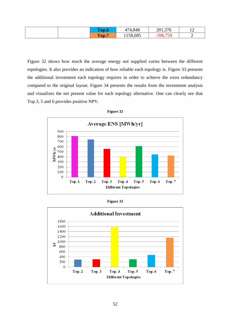
52
Top.6 474,848 201,376 12
Top.7 1158,685 -396,759 2
Figure 32 shows how much the average energy not supplied varies between the different
topologies. It also provides an indication of how reliable each topology is. Figure 33 presents
the additional investment each topology requires in order to achieve the extra redundancy
compared to the original layout. Figure 34 presents the results from the investment analysis
and visualizes the net present value for each topology alternative. One can clearly see that
Top.3, 5 and 6 provides positive NPV.
Figure 32
Figure 33
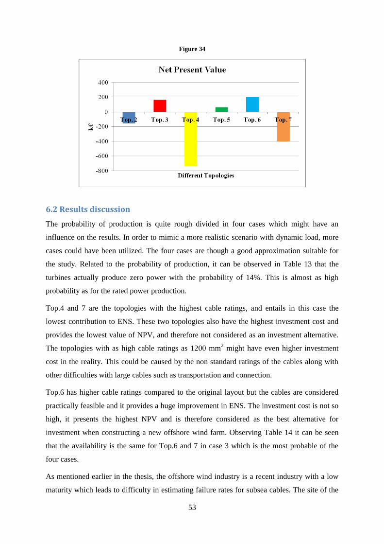
53
Figure 34
6.2 Results discussion
The probability of production is quite rough divided in four cases which might have an
influence on the results. In order to mimic a more realistic scenario with dynamic load, more
cases could have been utilized. The four cases are though a good approximation suitable for
the study. Related to the probability of production, it can be observed in Table 13 that the
turbines actually produce zero power with the probability of 14%. This is almost as high
probability as for the rated power production.
Top.4 and 7 are the topologies with the highest cable ratings, and entails in this case the
lowest contribution to ENS. These two topologies also have the highest investment cost and
provides the lowest value of NPV, and therefore not considered as an investment alternative.
The topologies with as high cable ratings as 1200 mm2 might have even higher investment
cost in the reality. This could be caused by the non standard ratings of the cables along with
other difficulties with large cables such as transportation and connection.
Top.6 has higher cable ratings compared to the original layout but the cables are considered
practically feasible and it provides a huge improvement in ENS. The investment cost is not so
high, it presents the highest NPV and is therefore considered as the best alternative for
investment when constructing a new offshore wind farm. Observing Table 14 it can be seen
that the availability is the same for Top.6 and 7 in case 3 which is the most probable of the
four cases.
As mentioned earlier in the thesis, the offshore wind industry is a recent industry with a low
maturity which leads to difficulty in estimating failure rates for subsea cables. The site of the

54
offshore wind farm is also of importance related to this because the largest contribution of
external influence on subsea cables is caused by anchors.
Failures are more likely to occur in the beginning- and in the end of the components life time
and the failures occurring in the early beginning after commissioning the offshore wind farm
have a high impact on the NPV.

55
CHAPTER 7: Conclusions
This chapter concludes the thesis, summarizes the results, present some ideas and discusses
future work.
7.1 Conclusions and discussion
The main objectives of this study were to evaluate different layouts for the internal grid of an
offshore wind farm with respect to reliability, investments and maintenance- and considering
cable constraints. For this analysis a model was constructed as a benchmark and the software
NEPLAN was utilized as a working tool. The aim of the presented results was to highlight
weak spots of the collector system and how different layouts with various cable ratings
contribute to a variety of ENS. Further aim of the presented results was to convert the possible
additional energy production into Euros and perform a cost benefit analysis. This is shown by
calculating the NPV and for the input data used in the report, three of the six investigated
topologies, i.e. Top.3, Top.5 and Top.6, had a positive NPV.
As stated previously in the report it is difficult to collect trustworthy reliability data and the
figures can vary extensively between manufacturers and construction sites offshore.
Installation cost and prices on different cable ratings and switchgear also vary between
manufacturers and over time with variations in metal prices. Another aspect to consider when
evaluating the results is fluctuations in income from produced electricity, where different
subsidies and the price per kilowatt hour vary over time. It is important to beware of all these
aspects when using the model for assessing the system performance and evaluating
investment alternatives.
7.2 Future work
For future studies it would be interesting to refine the model even more and include some
realistic and practical details. The model in this report does for example not consider practical
limitations and difficulties of using large cable dimensions. For very large cable dimensions it
could be problems with weight during transportation and installations of the cables. Another
aspect concerning large cable dimensions is the connection point, and the cables might have

56
to be reduced in dimension before connection. When using a cable loop in the middle like
Top.5, 6 and 7 it might need further investigation whether the connection point inside the
turbine is suitable for three connection points and additional switchgears.
Another aspect to investigate in future studies could be whether an increase in cable ratings
also could have more benefits over time with less risk of failure due to thicker layer of
insulation, less stress elicited by power flow and less power losses.
As a consequence of several parameters included in the model with uncertainties; a sensitivity
analysis should be performed. A sensitivity analysis can provide an indication of how
sensitive the results from the analysis are, when one or more input parameters changes in
values.
The constructed model for this study only consider to arrays with ten turbines and it would be
of interest to expand the model to include a complete wind farm with hundred turbines like
Thanet. In this case more topologies could be investigated and more than two arrays could be
connected together with loops in between. For such alternative it would be interesting to
include more statistical data in the model of for example how likely it is for failure to occur in
to arrays at the same time. The topology of e.g. Thanet may be more complex due to the
bathymetry and it could be interesting to investigate how such complexity may influence the
benefit of redundancy; however, this is a case per case situations.

57
References
[1] Billinton, R., Allan, R. N., Reliability evaluation of power system, Plenum Press, 2nd edition, 1996
[2] Billinton, R, Wenyuan, L. Reliability Assessment of Electric Power Systems Using Monte Carlo Methods,
Plenum Press, 1994.
[3] www.neplan.ch
[4] Presentation of Neplan reliability, Math Bollen, STRI AB, Ludvika, Sweden, 2007.
[5] Neplan User’s guide, Technical report.
[6] Frankén, B., STRI AB, Reliability study – Analyses of electrical system within offshore wind parks,
Technical report, Elforsk, 2007
[7] European Wind Energy Association, Oceans of Opportunity, Harnessing Europe’s largest domestic
energy resource, 2009
[8] Wizelius, T., Vindkraft i teori och praktik, Studentlitteratur, Sweden 2007
[9] Mousavi Gargari, S. Reliability Assessment of Complex Power Systems and the Use of NEPLAN Tool,
Master Thesis, Royal Institute of Technology, RCAM research team, 2006.
[10] Eriksson E. Wind farm layout, a reliability and investment analysis, Master Thesis, Uppsala University,
2008.
[11] Sannino A, Breder H, Kolby Nielsen E, Reliability of Collection Grids for Large Offshore Wind Parks,
2006
[12] Frankén, B., STRI AB, Reliability study – Analyses of electrical system within offshore wind parks,
Elforsk report, 2007
[13] www.vestas.com
[14] Tidwell J., Gaudiosi G., Offshore Wind Power, Multi-Science Publishing Co. Ltd, 2009.
[15] Besnard F., On Optimal Maintenance Management for Wind Power Systems, Licentiate Thesis, 2009.
[16] Blaabjerg F., Chen Z., Teodorescu R., Iov F., Power Electronics in Wind Turbine Systems, Aalborg
University, Institute of Energy Technology, 2006
[17] Holmstrøm, O. Reliability of state-of-the-art wind farms. Project UpWind, Technical report, 2007.
[18] Quinonez-Varela, G., Ault, G.W., Anaya-Lara, O., & McDonald, J.R. Electrical collector system options
for large offshore wind farms, 2007.
[19] DOE, EERE Web site. http://www.eere.energy.gov
[20] www.vattenfall.se

58
[21] www.siemens.com
[22] Download press photo: www.siemens.com/Transmission/pictures/EPT200809064, Rights for using the
picture has been received by Siemens AB Corporate Communications.
[23] powerplants.vattenfall.com/powerplant/thanet
[24] Offshore Wind in Europe, Energy & Natural resources, (pp.10), KPMG Market Report, 2010
[25] Manwell J.F., Mcgowan J.G., Rogers A.L., Wind Energy Explained Theory, Design and Application,
John Wiley & Sons Ltd, 2009.
[26] Discussion with Francois Besnard, Ph.D. student at Chalmers university of Technology and O&M analyst
at Vattenfall Wind.
[27] www.alpha-ventus.de
[28] Mason G., Development, Design and Construction of Offshore Windfarms, Presentation, 2009.
[29] Eugene F. Brigham, Michael C. Ehrhardt, Financial Management Theory and Practice, 2010.


