
1
SAINF:
A Toolbox for Analyzing the Effect of
Point-like, Line-like and Polygon-like Infrastructural Features
on the Distribution of Point-like Non-infrastructural Features
Version 2.3 – 1 Feb 2004
Atsuyuki Okabe* and Tohru Yoshikawa**
* Center for Spatial Information Science, University of Tokyo
** Department of Architecture and Building Science,
Tokyo Metropolitan University

2
PREFACE
This manual describes how to use SAINF: a toolbox for analyzing the effect of
infrastructural features on the distribution of point-like non-infrastructural features.
SAINF is part of the results obtained from the six year (1998-2003) project entitled
“Spatial Information Science for Human and Social Sciences” funded by the
Grant-In-Aid for Special Field Studies B, the Ministry of Education and Science, Japan.
The leader was Atsuyuki Okabe.
ACKNOWLEDGEMENTS
We express our thanks to Exceed Co. Ltd. for developing the program SAINF and to
Miki Arimoto for making the data of examples. This development was partly supported
by Grant-in-aid for Scientific Research No. 10202201 (Spatial information science for
human and social sciences) and No. 14350327 (Regional supporting network planning
for the elderly) provided by the Ministry of Education, Culture, Sports, Science and
Technology of Japan.

3
NOTICE
The authors distribute SAINF only to those who agree on the following conditions.
1. The user will use SAINF for nonprofit purposes only.
2. The authors will not bear responsibility for any trouble that the user may meet in the
use of SAINF.
3. When the user uses SAINF, he/she will report to the authors his/her name, affiliation,
address and e-mail address.
4. When the user publishes any results obtained by using SAINF, he/she will explicitly
state in the paper that he/she used SAINF. Also, he/she will send a reprint of the
paper to the authors.
5. The user will report to the authors any trouble he/she meets in the use of SAINF.
(The authors will remove bugs, if any, at their earliest convenience.)
The address of the authors is:
Atsuyuki OKABE
Center for Spatial Information Science
c/o Department of Urban Engineering, University of Tokyo
7-3-1 Hongo, Bunkyo-ku, Tokyo 113-8656, Japan

4
TABLE OF CONTENS
1. Introduction
2. Statistical methods used in SAINF
3. System requirements
4. Data setting
5. Installation of the SAINF software
6. Conditional nearest neighbor distance method
7. Cross K-function method
References

5
1. Introduction
In the real world we notice various kinds of phenomena such that the distribution of
one type of features is affected by the configuration of another type of features. For
example, fast-food stores tend to locate around stations; drugstores tend to locate
around hospitals; boutiques tend to locate along the main street; textiles factories tend
to locate near a river; high-class apartment buildings tend to locate around big parks;
lodging buildings for students tend to locate around university campuses. The
objective of this paper is to introduce a user-friendly GIS-based toolbox, called SAINF,
for analyzing these locational trends statistically.
About two decades ago, when researchers wanted to use quantitative methods for
spatial analysis, they had to develop computer programs by themselves. As a result,
the use of those methods was very limited. This limitation was resolved by the
emergence of user-friendly GIS in the late 1980’s. To incorporate this new technology
into spatial analysis, methodologies for linking spatial analysis to GIS were discussed
(Goodchild, 1987; Anselin and Getis, 1992; Anselin et al. 1992; Goodchild et al. 1992;
Fotheringham and Rogerson, 1994), and GIS-based toolboxes for spatial analysis
began to develop (Walker and Moor, 1988; Haslett et al. 1990; Openshaw et al. 1990;
Openshaw et al. 1991). At present many GIS-based toolboxes for spatial analysis are
available (Getis, 2000; Volume 2, No.1 of Journal of Geographical Systems), and they
are found at
http://www.csiss.org/clearinghouse/ (Center for Spatially Integrated Social Science);
http://ua.t.u-tokyo.ac.jp/okabelab/satools/.
The former site provides a powerful search engine for spatial tools, and the latter site
provides a web system for finding sites serving free software packages for spatial
analysis (the outline is shown in Itoh and Okabe (2003)).
Although many tools are found on the web space, they do not completely cover
methods for spatial analysis. The toolbox SAINF provides a tool for spatial analysis to
fill this gap. To introduce this tool explicitly, let us refer to two classifications. First,
we classify features into two types by the duration of life: ‘non-infrastructural’ features
or ‘infrastructural’ features. The non-infrastructural features mean the features that
usually last for a few decades or so. As referred to in the first paragraph, examples are:
fast-food stores, drugstores, boutiques, and apartment buildings. The infrastructural
features mean the features that last for one hundred years or more. Examples are:

6
stations, main streets, and big parks that are referred to in the first paragraph. The
toolbox SAINF is particularly useful for examining the effect of infrastructural
features on the distribution of non-infrastructural features. Considering this nature, we
name our toolbox SAINF (Spatial Analysis for the effect of INFrastructural features on
the distribution of non-infrastructural features). Note that we may also use SAINF
when distinction between non-infrastructure and infrastructure is not always clear (the
effects of two classes of features are bilateral, or the direction of the effects is
unknown). In this case, we may examine the effect in two directions: the effect of A
features on the distribution of B features and vice versa.
Second, we classify features into three types by size and shape: point-like features,
line-like features and polygon-like features. One of the most distinctive characteristics
of SAINF is that it can deal with the effect of not only point-like infrastructural
features but also line-like and polygon-like infrastructural features on the distribution
of non-infrastructural features. Note that since non-infrastructural features are mostly
point-like features, SAINF assumes that non-infrastructural features are point-like
features.

7
2. Statistical Methods Used in SAINF
SAINF employs two statistical methods: the conditional nearest neighbor distance
method (Okabe and Miki, 1984; Okabe and Fujii, 1994; Okabe et al., 1988; Okabe and
Yoshikawa, 1989), and the cross K-function method (Ripley, 1981). The conditional
nearest neighbor distance method is different from the ordinary nearest neighbor
distance method (Dacey, 1968), and the K-function method in SAINF is slightly
different from the ordinary one with respect to the boundary treatment. To show these
differences and for the ease of introducing SAINF, we briefly refer to these methods in
this section.
SAINF considers a bounded polygon, S , (representing a region) in which a set,
}...,,{ 1 nooO = , of geometrical objects (representing infrastructural features), and a set,
}...,,{ 1 mppP = , of points (representing non-infrastructural features) are placed. The
geometrical objects in O may be points, line segments or polygons. SAINF is
designed to test the following hypothesis.
Hypothesis O
H : points P are uniformly and randomly distributed over OS \ .
(Note that objects in O are not necessarily uniformly and randomly distributed on
S ; rather, usually they are non-uniformly distributed.)
The conditional nearest neighbor distance method has two tests: the average neighbor
distance test and the goodness-of-fit test. The former method uses the average nearest
neighbor distance, d , defined by
),(1
1
Opdm
dm
i
i
=
= , (1)
where )}},({min{mim),( ,...,1 qpdOpd ioqnji j== , i.e. the distance from i
p to the
nearest point in O . To use d as a test statistic, we need the probability density
function, g( d ), of d . In theory, this function is exactly obtained from the function
F(t) which indicates the area of the buffer ring of O whose width is t . The
derivation of F(t) is shown in Section 8.3.1 of Okabe et al. (2000). Once we obtain the
probability density function )(dg , we can exactly test the hypothesis O
H .

8
Alternatively, when m is large, we may approximate the probability density function
g( d ) by the normal distribution according to the central limit theorem, and we can use
the ordinary mean test. To be explicit, the test statistic, z , is given by
m
dz = . (2)
This follows the standard normal distribution.
The second test of the conditional nearest neighbor distance method is the
goodness-of-fit test defined by
=
=
k
i i
ii
mQ
mQN
0
22 )(
, (3)
where iQ is the probability that the distance from a point-like non-infrastructural
feature to its nearest neighbor infrastructural feature is in between i
a and 1+ia under
the hypothesis O
H , and i
N is the observed number (frequency) of the points of P
whose nearest neighbor distances are in between i
a and 1+ia .
SAINF also provides the cross K-function method for the point set O. Let )(tKi
be the
number of points in P whose nearest neighbor distance is less than or equal to t from the
i th point in O divided by the total number of points. Then the cross K-function K(t) is
given by
).(1
)(1
tKn
tK
n
i
i
=
= (4)
We can obtain the observed cross K-function )(tK from the method used in deriving
)(tF . Therefore we do not have to use the adjusting factor for the boundary effect. The
boundary effect is exactly taken into account. Comparing the observed cross K-function
)(tK and the expected cross K-function E( )(tK ), we can test the hypothesis O
H .

9
3. System requirements
Windows NT, 2000, (XP)
ArcView 8.2 or higher

10
4. Data Setting
SAINF uses three types of layers that are formatted in Shape files.
(1) The layer of infrastructural features.
Point-like infrastructural features such as stations are represented by points;
line-like infrastructural features such as streets are represented by lines;
polygon-like infrastructural features such as parks are represented by polygons.
(2) The layer of non-infrastructural features represented by points.
(3) The layer of a study area represented by a polygon.
For illustrative purposes, an actual example is used in which infrastructural features are
parks, non-infrastructural features are high-class apartment buildings (so called
“mansion” in Japanese), and the study region is the Kiba region in Tokyo.

11
5. Installation of the SAINF software
Obtain “ToolTemplate.mxd” (an empty ArcMap Document File including SAINF) from
the SAINF website and make its copy on your Windows PC where ArcView is
installed:
Start ArcMap by double clicking the copy of ToolTemplate.mxd and add the three
layers (data (1), (2) and (3) in Section 4) to the ArcMap Document File using the
AddData command.
A set of tools in SAINF is indicated by [SAINF Tools] on the left end of the ArcMap
menu bar at the top line of the window. Tools in this set are also shown by icons in the
sub-menu bar [SAINF Tools] placed on the window. You can start SAINF commands
by clicking one of these icons.

12
6. Conditional Nearest Neighbor Distance Method
6.1 Creation of buffer rings and trimming off the rings outside the study region
We are going to generate the buffer rings of infrastructural facilities (parks in our
example) and trim off the rings outside the study area.
6.1.1 Creation of buffer rings
We use one of the functions of ArcView, [buffer generation].
Open [Tools] in the ArcMap menu.
Click [Buffer Wizard] (Figure 6.1.1).
Figure 6.1.1

13
Then the dialog box shown in Figure 6.1.2 appears.
Figure 6.1.2
Click [The features of a layer].
Click the layer of infractructural features from the pull-down menu. In our case, the
layer of infrastructural features is “parks”.
Click [Next].
14
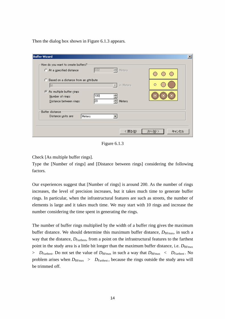
Then the dialog box shown in Figure 6.1.3 appears.
Figure 6.1.3
Check [As multiple buffer rings].
Type the [Number of rings] and [Distance between rings] considering the following
factors.
Our experiences suggest that [Number of rings] is around 200. As the number of rings
increases, the level of precision increases, but it takes much time to generate buffer
rings. In particular, when the infrastructural features are such as streets, the number of
elements is large and it takes much time. We may start with 10 rings and increase the
number considering the time spent in generating the rings.
The number of buffer rings multiplied by the width of a buffer ring gives the maximum
buffer distance. We should determine this maximum buffer distance, DBFmax, in such a
way that the distance, DFarthest, from a point on the infrastructural features to the farthest
point in the study area is a little bit longer than the maximum buffer distance, i.e. DBFmax
> DFarthest. Do not set the value of DBFmax in such a way that DBFmax < DFarthest . No
problem arises when DBFmax > DFarthest , because the rings outside the study area will
be trimmed off.

15
Type [Number of rings] and [Distance between rings].
Click [Next].
Then the dialog box shown in Figure 6.1.4 appears.
Figure 6.1.4
Click [Yes] for [Dissolve barriers between buffers?]
If the infrastructural features are polygons, check [only outside the polygon(s)] for
[Create buffers so that they are].
Click [In a new layer.] for [Where do you want the buffers to be saved?], and type a
new file name.
Click [Finish].

16
In a few minutes (or a few hours depending on the number of rings), the buffer rings are
indicated by “contour lines” as in Figure 6.1.5.
Figure 6.1.5

17
6.1.2 Trim off the buffer rings outside the study area
Click [Geoprocessing Wizard] in the [Tools] menu.
The dialog box shown in Figure 6.1.6 appears.
Figure 6.1.6
Click [Clip one layer base on another].
Click [Next].

18
The dialog box shown in Figure 6.1.7 appears.
Figure 6.1.7
Using the pull-down menu of [Select the input layer to clip:], click the buffer layer
generated in Section 6.1.1.
Using the pull-down menu of [Select a polygon clip layer], click our study region (e.g.
the Kiba region in Tokyo).
Using the pull-down menu of [Specify the output shapefile or feature class], type a file
name.
Click [Finish].

19
SAINF shows the buffer rings trimmed off the outside of the study region (the purple
colored area in Figure 6.1.8) and the resulting trimmed buffer rings are stored in the
above file.
Figure 6.1.8

20
6.2 Calculation of the distance from each non-infrastructural feature (a point) to
its nearest point on the infrastructural features
Open [SAINF Tools].
Click [NN Distance] (Figure 6.2.1).
Note that “NN Distance” means “Nearest Neighbor Distance”.
Figure 6.2.1

21
The dialog box [Infra feature layer] shown in Figure 6.2.2 appears.
Figure 6.2.2
Click a layer of infrastructural features, e.g. the layer of parks in our example.
Cick [OK].
The dialog box [Non-infra feature layer] shown in Figure 6.2.3 appears.
Figure 6.2.3
Click a layer of non-infrastructural features, e.g. “appartment2” in our case.
Click [OK].

22
The dialog box [Study region layer] shown in Figure 6.2.4 appears.
Figure 6.2.4
Click a study region, e.g. “study-region2” in our case.
Click [OK].
The dialog box [Do you want to visualize the lines from non-infra features to their
nearest infra features?] (Figure 6.2.5) appears.
Figure 6.2.5
If you want to visualize the line from each non-infrastructural feature to its nearest
infrastructural feature, click [Yes].

23
The lines are shown as in Figure 6.2.6.
Figure 6.2.6

24
When computation is done, the field named [NN Distance] is added to the
non-infrastructural feature layer (Figure 6.2.7).
Figure 6.2.7

25
6.3 Calculation of the average distance from non-infrastructural features to their
nearest infrastructural features
Click [Average NN distance] in the [SAINF Tools] menu (Figure 6.3.1).
Figure 6.3.1

26
The dialog box [Non-infra feature layer] shown in Figure 6.3.2 appears.
Figure 6.3.2
Click one type of non-infrastructural features, e.g. parks in our case.
Click [OK].
When the computation completes, the average nearest neighbor distance and the number
of non-infrastructural features are shown (Figure 6.3.3). In our case, the former is
516.79, and the latter is 204. These numbers are denoted by d and m , respectively.
Figure 6.3.3

27
6.4 The mean and the standard deviation of the distance from a random point to
its nearest infrastructural feature
Click [Mean & Standard Deviation] in the [SAINF Tools] menu (Figure 6.4.1).
Figure 6.4.1

28
The dialog box [Select a buffer layer] shown in Figure 6.4.2 appears.
Figure 6.4.2
Click the layer created in Section 6.1.2 (in our case, “Clip Output 6”), and Click [OK].
Then the total area of the buffer rings, the longest buffer distance and the width of a
buffer ring are shown (Figure 6.4.3).
Figure 6.4.3
Click [OK] and then, in a few minutes of computation, SAINF gives the mean, μ , and
the standard deviation, , of the distance from a random point to the nearest point in
infrastructural features (Figure 6.4.4). Note these figures on your memo pad. In our case,
μ =556.841 and =375.811.
Figure 6.4.4

29
6.5 Analysis with the average nearest neighbor distance test
In Section 6.3, we have obtained the observed average nearest neighbor distance, d =
516.79 for =m 204 non-infrastructural features. In Section 6.4, we have obtained the
expected nearest neighbor distance, μ = 556.841, and its standard deviation =
375.811 under the null hypothesis 0
H (i.e. non-infrastructural features are uniformly
and randomly distributed over a study region). Comparing d = 516.79 with μ =
556.841, we notice that apartment buildings (non-infrastructural features) tend to locate
near parks in Kiba. To test this tendency statistically, we employ the mean test. To be
explicit, the test statistic, z , is given by equation (2) in Section 2. In our case, z =
-1.52216. Therefore the null hypothesis cannot be rejected with confidence level 95%.
The above tendency is statistically weak.

30
6.6 Analysis with the goodness-of-fit test
An alternative test is the goodness-of-fit test. The method is shown in Section 2. This
test is to compare the observed number of non-infrastructural features (e.g. high-class
apartment buildings) in each interval with the expected number under the null
hypothesis O
H (i.e. non-infrastructural features are uniformly and randomly
distributed over a study region).
6.6.1 A file for ring intervals
Make a file that shows ring intervals (i.e. k
aa ,,0
K in equation 3) using a text editor,
such as Notepad in Windows. The first term 0
a is fixed 0 and k
a should exceed the
longest distance of the buffer rings obtained in Section 6.4. The width of each interval
may be different, but the width should be the width fixed in Section 6.1 multiplied by a
natural number. An example is:
0
300
600
900
1200
1800

31
6.6.2 Calculation of the area of each buffer ring
When the null hypothesis O
H holds, the expected number of non-infrastructural
features in a buffer ring is proportional to its area. To calculate this area, click [Areas of
buffer rings] in the [SAINF Tools] menu (Figure 6.6.1).
Figure 6.6.1
Then the dialog box shown in Figure 6.6.2 appears.
Figure 6.6.2

32
Click the layer made in Section 6.1.2 and click [OK].
Then the dialog box shown in Figure 6.1.3 appears.
Figure 6.6.3
Type the file name made in Section 6.6.1 in the first row, type the name of a new file
for storing the results in the second row, and click [OK].
When the computation is done, the results are written in the file as follows:
Notes: 0,100,S(1),12300 stands for that the area of S(1), in which X is larger than 0, and
smaller than and equal to 100, is 12300.
0,300,S(1),1792534.951
300,600,S(2),1817824.723
600,900,S(3),1362014.769
900,1200,S(4),690877.662
1200,1800,S(5), 415054.818
The total amount of sum of area calculations = 6078306.923

33
6.6.3 Counting the observed number of non-infrastructural features in each ring
Click [Number of non-infra features in rings] in the [SAINF Tools] menu (Figure
6.6.4).
Figure 6.6.4
The dialog box shown in Figure 6.6.5 appears.

34
Figure 6.6.5
Click the layer of non-infrastructural features (e.g. high-class apartment buildings).
Click [OK].
Then the dialog box shown in Figure 6.6.6 appears.
Figure 6.6.6
Click the layer of the study region (e.g. study-region2).
Click [OK].
Then the dialog box shown in Figure 6.6.7 appears.
Figure 6.6.7
Type the name of the file made in Section 6.6.1 in the first row, type the name of a new
file for the results in the second row, and click [OK].
35
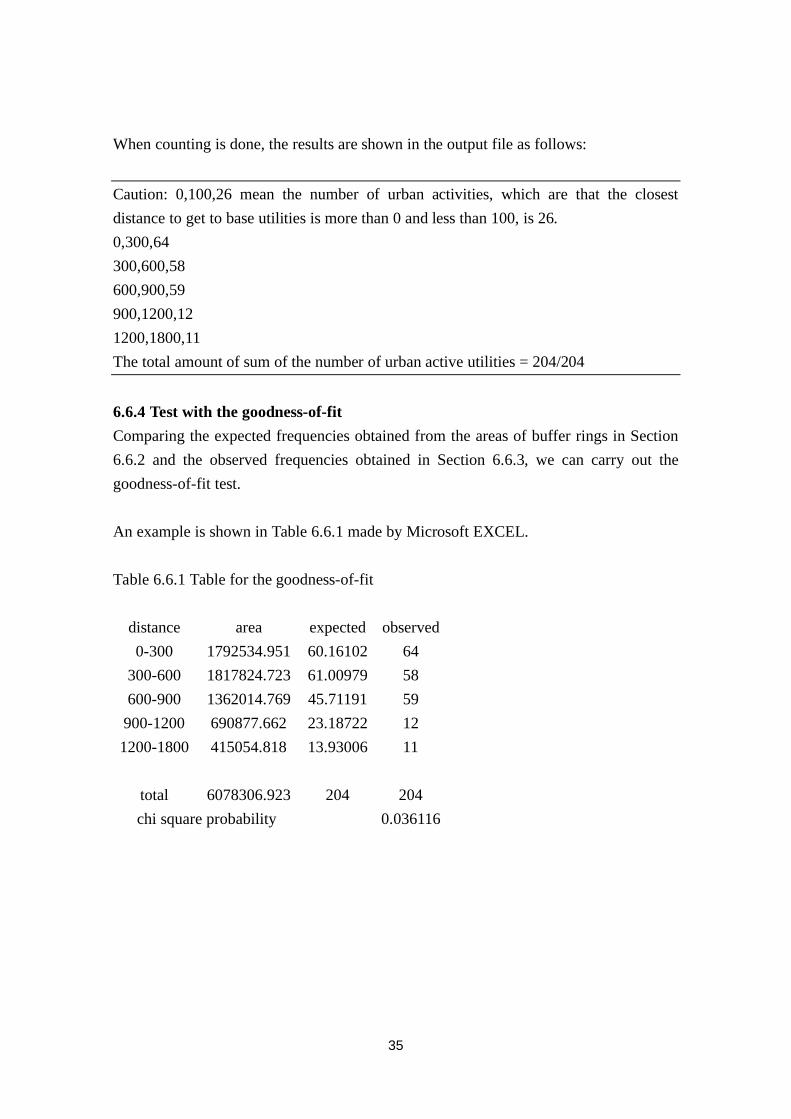
When counting is done, the results are shown in the output file as follows:
Caution: 0,100,26 mean the number of urban activities, which are that the closest
distance to get to base utilities is more than 0 and less than 100, is 26.
0,300,64
300,600,58
600,900,59
900,1200,12
1200,1800,11
The total amount of sum of the number of urban active utilities = 204/204
6.6.4 Test with the goodness-of-fit
Comparing the expected frequencies obtained from the areas of buffer rings in Section
6.6.2 and the observed frequencies obtained in Section 6.6.3, we can carry out the
goodness-of-fit test.
An example is shown in Table 6.6.1 made by Microsoft EXCEL.
Table 6.6.1 Table for the goodness-of-fit
distance area expected observed
0-300 1792534.951 60.16102 64
300-600 1817824.723 61.00979 58
600-900 1362014.769 45.71191 59
900-1200 690877.662 23.18722 12
1200-1800 415054.818 13.93006 11
total 6078306.923 204 204
chi square probability 0.036116

36
7. Cross K-function method
7.1 Cross K-function
The cross K-function is defined by equation (4) in Section 2. Detailed illustration of this
function is found, for example, in Ripley.
7.2 General setting
The cross K-function in SAINF assumes:
(1) infrastructural features are point-like features (e.g. stations in a city),
(2) As is seen in Figure 7.2.1, the layer of a study region includes the field named
“Area”. If the layer does not include it, open the attribute table of the layer of the
study region and add the field named “Area” by clicking [option] and [add field].
Figure 7.2.1

37
7.3 Estimation of the cross K-function
Click [Cross K-function] in the [SAINF Tools] (Figure 7.3.1).
Figure 7.3.1
The dialog box shown in Figure 7.3.2 appears. Click a layer of infrastructural features,
for example, “stations”, and click [OK].
Figure 7.3.2

38
Then the dialog box shown in Figure 7.3.3 appears.
Click a layer of non-infrastructural features, for example, “apartment2” (implying
high-class apartment buildings), and click [OK].
Figure 7.3.3
Then the dialog box shown in Figure 7.3.4 appears. Click a layer of a study region, for
example, “study-region2”, and click [OK]. If this layer does not contain the field named
“Area”, an error message appears. See Section 7.2.
Figure 7.3.4

39
Then the dialog box shown in Figure 7.3.5 appears. Type a new file name for output and
click [OK].
Figure 7.3.5
Usually it takes twenty minutes or so for computing the K-function. When the
computation is done, the message shown in Figure 7.3.6 appears.
Figure 7.3.6
40
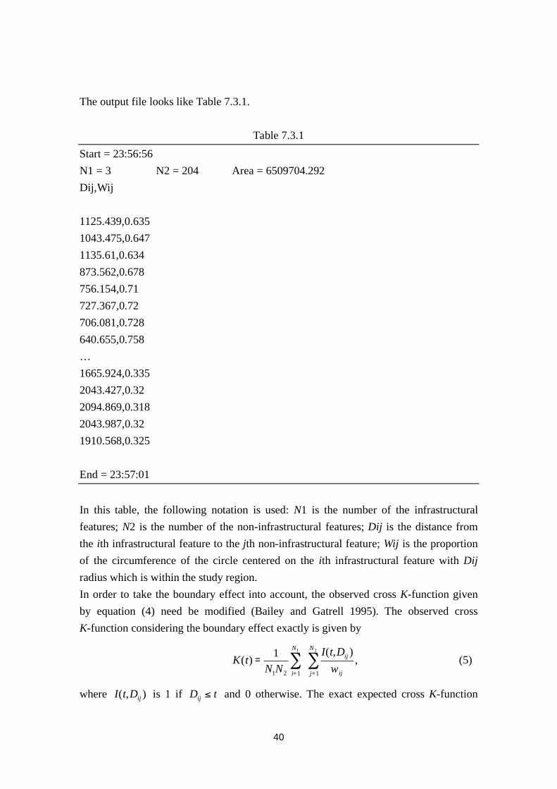
The output file looks like Table 7.3.1.
Table 7.3.1
Start = 23:56:56
N1 = 3 N2 = 204 Area = 6509704.292
Dij,Wij
1125.439,0.635
1043.475,0.647
1135.61,0.634
873.562,0.678
756.154,0.71
727.367,0.72
706.081,0.728
640.655,0.758
…
1665.924,0.335
2043.427,0.32
2094.869,0.318
2043.987,0.32
1910.568,0.325
End = 23:57:01
In this table, the following notation is used: N1 is the number of the infrastructural
features; N2 is the number of the non-infrastructural features; Dij is the distance from
the ith infrastructural feature to the jth non-infrastructural feature; Wij is the proportion
of the circumference of the circle centered on the ith infrastructural feature with Dij
radius which is within the study region.
In order to take the boundary effect into account, the observed cross K-function given
by equation (4) need be modified (Bailey and Gatrell 1995). The observed cross
K-function considering the boundary effect exactly is given by
K(t) =1
N1N2 i=1
N1 I(t,Dij )
wijj=1
N2
, (5)
where I(t,Dij ) is 1 if Dij t and 0 otherwise. The exact expected cross K-function

41
under the null hypothesis O
H , E( )(tK ), is given by
E(K(t)) = t 2 . (6)
By comparing these two functions, we can test the null hypothesis O
H .

42
References
Bailey, T.C. and Gatrell, A.C., (1995) Interactive Spatial Data Analysis, Harlow:
Longman.
Dacey, M.F., (1968) Two-Dimensional Random Point Patterns, A Review and an
Interpretation, Papers of the Regional Science Association, Vol.13, pp.41-55
Okabe, A., Boots, B., Sugihara, K. and Chiu, S.N. (2000) Spatial Tessellations:
Concepts and Applications of Voronoi Diagrams, 2nd
edition, Chichester: John Wiley.
Okabe, A. and Fujii, A., (1984) "The Statistical Analysis through a Computational
Method of a Distribution of Points in Relation to Its Surrounding Network",
Environment and Planning A, Vol.16, pp.107-114
Okabe, A. and Miki, F., (1984) "A Conditional Nearest-Neighbor Spatial Association
Measure for the Analysis of Conditional Locational Interdependence", Environment
and Planning A, Vol.16, pp.163-171.
Okabe, A. and Yoshikawa, T., (1989) "Multi Nearest Distance Method for Analyzing
the Compound Effect of Infrastructural Elements on the Distribution of Activity
Points", Geographical Analysis, Vol.21, No.3, pp.216-235
Okabe, A., Fujii, A., Oikawa, K. and Yoshikawa, T., (1988) "The Statistical Analysis of
a Distribution of Activity Points in Relation to Surface-Like Elements", Environment
and Planning A, Vol. 20, pp.609-620.
Ripley, B.D., (1981) Spatial Statistics, Chichester: John Wiley.


