Download - Signal processing for atmospheric radars

NCAR/TN-331+STRNCAR TECHNICAL NOTE
May 1989
Signal Processing
for Atmospheric Radars
R. Jeffrey KeelerRichard E. Passarelli
ATMOSPHERIC TECHNOLOGY DIVISION
NATIONAL CENTER FOR ATMOSPHERIC RESEARCHBOULDER, COLORADO
-
iI


TBSIE OF COTENTS
TABLE OF CONTENTS ..................... . iii
LIST OF FIGURES ......................... v
LIST OF TABLES ................... . .. .vii
PREFACE. .. .. i.......................
1. Purpose and scope ................. 1
2. General characteristics of atmospheric radars. 32.1 Characteristics of processing .......... 32.1.1 Sampling ................... 32.1.2 Noise ...... ............... 42.1.3 Scattering ............... 52.1.4 Signal to noise ratio (SNR) .......... 62.2 Types of atmospheric radars .......... 62.2.1 Microwave radars . ........... 72.2.2 ST/MST radars or wind profilers ....... 82.2.3 FM-CW radars .. .............. 82.2.4 Mobile radars ............ .. 92.2.5 Lidar ............ ....... 102.2.6 Acoustic sounders . .......... 11
3. Doppler power spectrum moment estimation . .... 133.1 General features of the Doppler power spectrum. 143.2 Frequency domain spectral moment estimation . 183.2.1 Fast Fourier transform techniques . .... 183.2.2 Maximum entropy techniques .......... 203.2.3 Maximum likelihood techniques . ....... 233.2.4 Classical spectral moment computation ..... 253.3 Time domain spectral moment estimation. ..... 273.3.1 Geometric interpretations ........... 273.3.2 "Pulse pair" estimators ........... 283.3.3 Circular spectral moment computation for
sampled data. . ............. 313.3.4 Poly pulse pair techniques ..... 333.4 Uncertainties in spectrum moment estimators . . 353.4.1 Reflectivity. ... ............ 353.4.2 Velocity. . . ..... .. ..... 363.4.3 Velocity spectrum width ........... 37
4. Signal processing to eliminate bias and artifacts. 434.1 Doppler techniques for ground clutter suppression 434.1.1 Antenna and analog signal considerations. ... 444.1.2 Frequency domain filtering. ......... 454.1.3 Time domain filtering ............. 464.2 Range/velocity ambiguity resolution ....... 504.2.1 Resolution of velocity ambiguities ...... 51
iii

4.2.2 Resolution of range ambiguities ....... 554.3 Polarization switching consequences ....... 56
5. Exploratory signal processing techniques . .... 575.1 Pulse compression .... .......... 575.1.1 Advantages of pulse compression . ...... 585.1.2 Disadvantages of pulse compression. ...... 595.1.3 Ambiguity function. .. 615.1.4 Comparison with multiple frequency scheme . 635.2 Adaptive filtering algorithms ......... 635.2.1 Adaptive filtering applications ....... 645.2.2 Adaptive antenna applications .. ..... 685.3 Multi-channel processing. ............ 695.4 A priori information. ............. 70
6. Signal processor implementation ......... 716.1 Signal processing control functions ..... 716.2 Signal Z?D conversion and calibration ...... 746.3 Reflectivity processing ... .......... 766.4 Thresholding for data quality ......... 78
7. Trends in signal processing. ............ 817.1 Realization factors ............... 817.1.1 Digital signal processor chips ....... 817.1.2 Storage media ................. 827.1.3 Display technology . .............. 837.1.4 Commercial radar processors .......... 837.2 Trends in programmability of DSP. ........ 847.3 Short term expectations .......... .... 857.3.1 Range/velocity ambiguities ......... 857.3.2 Ground clutter filtering .......... 867.3.3 Waveforms for fast scanning radars ...... 867.3.4 Data compression. ............. 877.3.5 Artificial intelligence based feature extraction 877.3.6 Real time 3D weather image processing .. ... 877.4 Long term expectations . ............ 877.4.1 Advanced hardware ...... . .. 887.4.2 Optical interconnects and processing ..... 887.4.3 Communications . . . . . . . . . . . . . . . . 887.4.4 Electronically scanned array antennas ..... 887.4.5 Adaptive systems ............... 89
8. Conclusions. . ................... 918.1 Assessment of our past. ............. 918.2 Recommendations for our future . ........ 928.3 Acceptance of new techniques ........... 938.4 Acknowledgements. .............. 93
ACRONYM LIST ........................... 95
BIBLIOGRAPHY ....... ........... .... . . 97
iv

TIST OF FJIGRES
Fig 3.1 Doppler power spectrum (128 point periodogram) of 15typical weather echo in white noise. Estimatedparameters are velocity ~ 0.4 Vax velocity spectrumwidth ~ .04 Vmax, and SNR 10 dB.
Fig 3.2 Three dimensional representation of the complex 29autocorrelation function as a helix. Radius of helixRs(0) is proportional to total signal power, Ps;rotation rate of helix is proportional to velocity, V;width of envelope is inversely proportional to velocityspectrum width, W. Delta function Rn(0) representsnoise power.
Fig 3.3 Periodogram power spectrum plotted on unit circle in the 32z-plane. Note velocity aliasing point, the Nyquistvelocity, at z=-l.
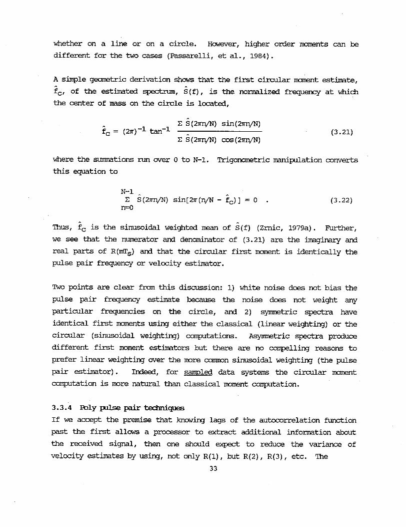
Fig 3.4 Comparison of classical and circular (pulse pair) first 34moment estimators. Classical estimate is determined bylinear weighting of spectrum estimate and circularestimate, by sinusoidal weighting.
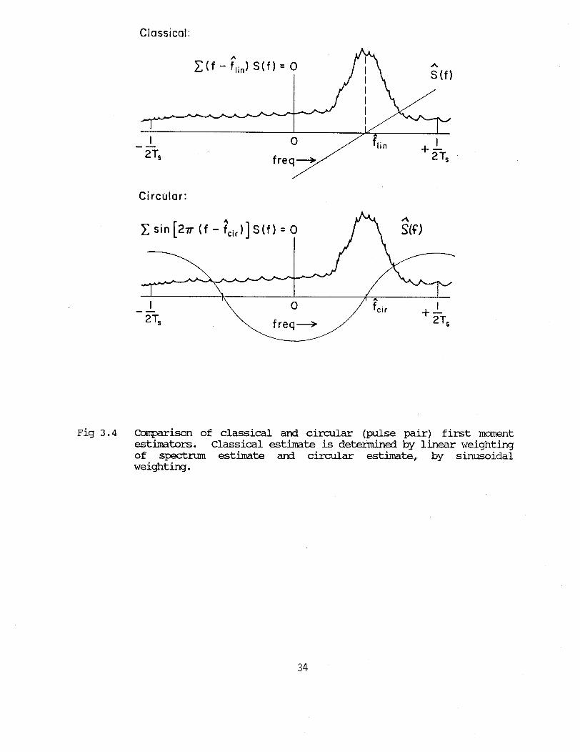
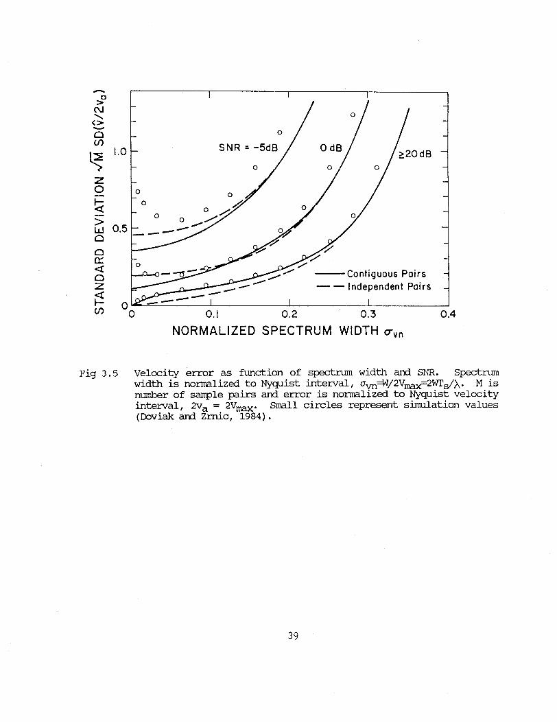
Fig 3.5 Velocity error as function of spectrum width and SNR. 39Spectrum width is normalized to Nyquist interval,vn=W/2Vmx=2WTs/X. M is number of sample pairs and
error is normalized to Nyquist velocity interval, 2va =2Vmax. Small circles represent simulation values(Doviak and Zrnic, 1984).
Fig 3.6 Width error as a function of spectrum width and SNR. 42Spectrum width is normalized to Nyquist interval,
vn=W/2Vmax=2Wrs/X. M is number of sample pairs anderror is normalized to Nyquist interval, 2Vmax. Smallcircles represent simulation values (Doviak and Zrnic,1984).
Fig 4.la Clutter filter frequency response for a 3 pole infinite 47impulse response (IIR) high pass elliptic filter. Forground clutter width of 0.6 ms- 1 and scan rate of 5 rpmthis filter gives about 40 dB suppression. V = stopband. Vp = pass band cutoff, Vmax = 16 ms- (Hamidiand Zrnic, 1981).
Fig 4.lb Implementation of 3rd order IIR clutter suppression 48filter; z-1 is 1 PRT delay. K1 - K4 are filter coeffi-cients (Hamidi and Zrnic, 1981).
v

Fig 5.1 Ambiguity diagram for single FM chirped pulse waveform 62with TB=10. T is range dimension. 0 is velocitydimension. Targets distributed in (r,q) space contributeto the filter output proportional to the ambiguityfunction. For atmospheric targets, Doppler shiftfrequencies are typically very small relative to pulsebandwidth (Rihaczek, 1969).
Fig 5.2 Prediction error surface for 2 weight adaptive filter. 65The LMS algorithm estimates the negative gradient of thequadratic error and steps toward the minimum mean squareerror (mse). The optimum weight vector is W* = (0.65,-2.10). If the input statistics change so that theerror surface varies with time, the adaptive weightswill track this change (Widrow and Stearns, 1985).
Fig 5.3 Adaptive filter structure. The desired response (dk) is 66determined by the application. The adaptive filter.coefficients (Wk) and/or the output signal (Yk) are theparameters used for spectrum moment estimation (Widrowand Stearns, 1985).
Fig 6.1 Block diagram of a typical signal processor. 26
vi

LSTr OF TAHBI
Table 1 Comparison of remote sensor sampling schemes and rates. 7
Table 2 Characteristics of several popular windows when applied 20to time series data analysis (Marple, 1987).
Table 3 Expressions for variance of velocity estimators at high 38SNR. Assumes Gaussian spectra in white noise, lownormalized velocity width (Wn=W/2Vmx) and large M.Expressions apply to both pulse pair and Fouriertransform estimators.
Table 4 Expressions for variance of width estimators at high 41SNR. Assumes Gaussian spectra in white noise, lownormalized velocity width (Wn=W/2Vmax) and large M.Expressions apply to both pulse pair and Fouriertransform estimators.
vii


PiRFACE
This review of signal processing for atmospheric radars was originally
written as Chapter 20 of the book Radar in Meteorology, edited by Dave Atlas
(1989) for the Proceedings of the 40th Anniversary and Louis Battan Memorial
Radar Meteorology Conference. We have attempted to give the reader an
overview of signal processing techniques and the technology that are
applicable to the atmospheric remote sensing tools of weather radar, lidar,
ST/MST radars and wind profilers.
This NCAR Technical Note includes the signal processing chapter and the
relevant references in a single document. The text has had minor editing
and the references have been slightly expanded over the version published in
Radar in Meteorology.
We hope that this Technical Note will assist the many individuals who want a
better understanding of signal processing to achieve that goal.
R. Jeffrey Keeler
Richard E. Passarelli
March 1989
ix
1. PURPOSE AND SODFE
Signal processing is perhaps the area of atmospheric remote sensing where
science and engineering make their point of closest contact. Signal
processing offers challenges to engineers who enjoy developing state-of-the-
art systems and to scientists who enjoy being at the crest of the wave in
observing atmospheric phenomena in unique ways.
The primary function of radar signal processing is the accurate, efficient
extraction of information from radar echoes. A typical pulsed Doppler radarsystem samples data at 1000 range bins at 1 kilohertz pulse repetition
frequency (PRF), generating approximately 3 million samples per second
(typically in-phase (I) and quadrature phase (Q) components from a linear
channel and often a log receiver). These "time series", in their raw form,
convey little information that is of direct use in determining the state of
the atmosphere. The volume of time series data is sufficiently large that
storage for later analysis is impractical except for limited regions of time
and space. The data must be processed in real time to reduce its volume and
to convert it to more useful form.
In this paper the current state of signal processing for atmospheric radars
(weather radars, ST/MST radars or wind profilers, and lidars) shall be
discussed along with how signal processing is currently optimized for
various applications and remote sensors. The focus shall be on signal
processing for weather radar systems but the techniques and conclusions
apply equally well to ST/MST radars and lidars. Zrnic (1979a) has given an
excellent review of spectral moment estimation for weather radars and
Woodman (1985) has done the same for MST radars. Problem areas and
promising avenues for future research shall be identified. Finally, we
shall discuss the scientific and technological forces that are likely to
shape the future of atmospheric radar signal processing.
We will differentiate between "signal processing" (the topic of this review)
and "data processing" in the following way. "Signal processing" is that set
1

of operations performed on the analog or digital signals for efficiently
extracting desired information or measuring some attribute of the signal.
For atmospheric radars this information is often referred to as the "base
parameter estimates". Fundamental base parameters are:
Radar reflectivity factor Z dBZRadial velocity V ms- 1
Velocity spectrum width1 W ms-l
In the course of extracting these estimates, signal processing algorithms
will improve the signal to noise ratio (SNR) through filtering or averaging,
mitigate the effects of interfering echoes such as ground clutter, remove
ambiguities such as range or velocity aliasing, and reduce the input data
rate by a significant factor. The end result of an effective signal
processing scheme is to provide minimum mean squared error estimates of the
base parameters along with the expected error or a measure of the degree of
confidence that can be placed on the estimates (e.g., the SNR). Note that
signal processing is primarily used in atmospheric remote sensing as an
estimation procedure as well as a detection process as in some aviation
applications. The emphasis is on making estimates of atmospheric parameters
or meteorological events.
"Data processing", on the other hand, takes up where signal processing
leaves off -- although the line of demarcation is not razor sharp. Data
processing algorithms take the base parameter estimates and further process
them so that they convey information that is of direct use to the radar
user. For example, data processing techniques imply display generation,
data navigation to a desired coordinate system, wind profile analyses, data
syntheses from several Doppler radars or other sensors, applying physical
constraints to the measured data, and forecasts or "nowcasts" of severe
weather hazards. Many aspects of data processing are covered in other
chapters.
1 The width is defined as the square root of the secondcentral moment of the spectral power distribution.
2

2. GENRA CIRACJERSLR'LCS OF AICMY4SERIC RADARS
There are two main classes of "radar" -- electromagnetic and acoustic.
Electromagnetic radars include microwave, UHF, VHF, infrared and optical
systems. Acoustic radars are only briefly described here. The signal
processing techniques employed for all these systems are similar (Serafin
and Strauch, 1978).
2.1 ClARACTERISTICS OF IRDCESSING
Although the processing techniques are nearly identical for the various
atmospheric radars, the way in which this backscattered or partially
reflected radiation is sampled, the principle noise sources, and the nature
of the scattering mechanisms are different.
2.1.1 Sampling
Because electromagnetic radars employ wavelengths from several meters to
less than 1 im, they must use different sampling techniques. There are two
constraints on the sample time spacing (Ts) of the backscattered signal.
The first is that the backscattered signal should be coherent from sample-
to-sample, i.e., the motion among the scatterers should be small compared to
the wavelength so that their relative positions produce highly correlated
echoes from sample-to-sample. The nominal duration of this correlation is
called the coherence time (Nathanson, 1969), i.e.,
Ts < tcoh = /4rW (2.1)
where the true velocity spectrum width W in ms-1 is a direct measure of the
relative motions of the scatterers. The coherence time is a measure of the
maximum time between successive samples for coherent phase measurements.
Thus, for short wavelength systems, such as a lidar, the backscattered
signal must be sampled much more rapidly than for a longer wavelength
microwave system. The autocorrelation function (defined later) can provide
a direct measure of the coherence time of a fluctuating target echo.
3

The second constraint on sampling is that for regularly spaced pulses, the
sampling frequency must be at least twice the maximum desired Doppler shift
frequency which reduces the occurrence of velocity aliasing. In this case
the time between samples is governed by,
Ts < tNyq = 4V' (2.2)
where tNyq is the minimum time between samples such that the desired
velocity V' is at least the so-called Nyquist velocity. Since V' is
typically much larger than W, the latter constraint usually dominates the
sampling requirement. In fact, if we assume the desired maximum velocity is
+ 25 ms-1 , then Ts V/100 or PRF = 100/ \ is a useful rule of thumb.
2.1.2 Noise
One of the goals of signal processing is to suppress the effects of noise.
The main source of noise in microwave radar is thermal in nature. This noise
power is simply
Pn = k Tsys Bsys (2.3)
where k is Boltzman's constant (1.38 x 10⁻²³ W/Hz/°K), Tsys is the total
system temperature, and Bsys is the total system bandwidth including effects
of preselector filters, IF filters, and all other amplifiers in the signal
path (Skolnik, 1970, 1980; Paczowski and Whelehan, 1988). With recent
improvements in low noise amplifiers (INA's), little room is left for
sensitivity improvement in conventional radar receivers. Presently, most
microwave radar systems are sufficiently sensitive that thermal radiation
from the earth makes a strong contribution to the receiver input at low
elevation angles.
ST/MST radar noise, because of its lower frequency, has a large contribution
from environmental, cosmic and atmospheric sources, and is not easily
quantified (Rottger and Larsen, Chap 21A). Therefore, antenna design and
the specific radar location and frequency band of operation define the
system noise.
4
Coherent lidar systems utilize detection schemes using optical heterodyning
onto cryogenic detectors with a local oscillator laser having relatively
high power mixing with the weak atmospheric return (Jelalian, 1980,
1981a,b). Because of the small wavelengths, quantum effects dominate the
detection process associated with random photon arrivals impacting the LD
laser. This "shot noise" contribution is a fundamental physical limitation
of lidar sensitivity.
2.1.3 Scattering
Atmospheric radars respond to a variety of scattering targets--
precipitation, cloud particles, aerosols, refractive index variations,
chaff, insects, birds, and ground targets. Probert-Jones (1962) derived the
familiar radar equation most often used by radar meteorologists for
precipitation scattering. A detailed derivation can be found in Doviak and
Zrnic (1984), Battan (1973), or Atlas (1964). The received power is
Pt G2 02 cTr 3 1k12 Ze L (2.4)Pr=
1024 ln2 X2 R2
This equation includes L, the product of several small but significant loss
terms which are necessary to accurately estimate radar reflectivity factor,
e.g. receiver filter loss, propagation loss, blockage loss, and processing
bias. Zric (1978) defines the receiver filter loss as that portion of the
input signal frequencies not passed by the finite receiver bandwidth,
typically 1-3 dB. The other losses depend on atmospheric conditions and
antenna pointing and are enumerated in Skolnik (1980). This equation is
correct for Rayleigh scattering of a distributed target that completely
fills the resolution volume. Non-Rayleigh targets or partially filled
resolution volumes will give received power estimates that cannot accurately
be related to precipitation rate. Rottger and Larsen (Chap. 21A) and
Huffaker, et al. (1976, 1984) give similar received power expressions for
returns from refractive index variations and from lidar aerosol returns,
respectively.
5

The required dynamic range for measuring the backscattered power from
atmospheric targets is very large because:
1. The effective backscatter cross-sections of atmospheric scatterers span
dynamic ranges of approximately 60 dB for precipitation but much larger
if cloud particle, "clear air", and ground target returns are included.
2. The R 2 dependence of the received power for distributed targets spans
a range of 50 dB between 1 and 300 km.
Microwave systems should accommodate the sum of these two effects and
typically can achieve a dynamic range of order 100 dB for power measurements
using either a log receiver, linear receiver with AGC, or some combination
of these.
2.1.4 Signal to noise ratio (SNR)
The ratio of the received signal power to the measured noise power is
defined to be the signal to noise ratio (SNR):
SNR = Pr/Pn (2.5)
The SNR is extremely important for analyzing tradeoffs in signal processing.
It is a key term along with spectrum width and integration time in analytic
evaluation of spectrum moment errors.
2.2 YPES OF AM[SHFERIC RAIDRS
A summary of the characteristics of the different types of electromagnetic
radars in use today for atmospheric research is discussed below. Table 1
assembles these differences.
6

Table 1
Remote Sensor Sampling Comparison
Pulse SampleSensor Wavelength Scatterers Beamwidth Duration Rate
(deg) (~sec) (Hz)RadarS-band 10cm Precipitation 0.5-3 0.25-4 103Ka-band 1 cm Precipitation 0.5-2 0.25-1 104mm-band 1 mm Cloud 0.2-1 0.25-1 105
ST/MST (profilers)UHF 75 cm Refractive 3-10 0.2-5 104->102VHF 6 m index 3-10 0.2-5 103->10
LidarIR 10 gmi Aerosols 0.01 0.1-3 107Optical <1 im Molecules (near field) <1
2.2.1 Microwave radars
Microwave pulsed radars radiate fields with wavelengths between 20 cm and 1
mm and are commonly used as "weather radars" (Smith, et al., 1974; Doviak,
et al., 1979). Depending on the wavelength, primary scattering is from
precipitation, insects (Vaughan,1985), refractive index fluctuations, and
cloud particles. Beams are typically circular in cross section with widths
0.5 to 3 degrees and the maximum usable ranges for storm observation is 200-
500 km. After a few kilometers range, the pulse volume is "pancake" shaped,
i.e., the pulse depth in range is small compared to the distance across the
beam. Attenuation effects range from severe for millimeter wavelength
systems, to nearly insignificant for 10 cm S-band systems.
Most centimeter wavelength microwave systems collect coherent samples over
several milliseconds. Millimeter wavelength radars can make use of the
double pulsing technique (Campbell and Strauch, 1976) to assure coherence
and to reduce an otherwise intolerable range ambiguity problem. Doviak and
Zrnic (1984) and Strauch (1988) have shown that since only the second pulse
of a double pulsing radar may be contaminated by overlaid echo from the
first pulse of the pair, only random errors occur in the pulse to pulse
correlations. These random errors may change very slowly with time so they
would appear to be systematic (bias) errors at a given time.
7

2.2.2 ST/ST radars or wind profilers
VHF and UHF radars which probe the mesosphere, stratosphere and/or the
troposphere are called ST/MST radars and sometimes known as wind profilers,
observe radial winds at wavelengths between 30 cm and 6 m at near vertical
incidence (Gage and Balsley, 1978; Rottger, et al., 1978). Scattering is
from atmospheric refractive index fluctuations in space, analogous to Bragg
scattering. Beamwidths may be as large as several degrees for tropospheric
sounding, but much narrower beams are used for longer stratospheric and
mesospheric ranges (Rottger and Larsen, Chap. 21A; Gage, Chap. 28A).
For a nominal 1 m wavelength, the atmospheric coherence time is typically
large fractions of a second. Consequently, the sampling rate to achieve
coherence is of order 10 Hz. Because of this and the typically weak clear
air returns, it is advantageous to perform time domain averaging of the
samples from pulse-to-pulse, e.g., at a given range, N successive complex
samples are averaged to yield a single complex pair. This operation
effectively reduces the sampling frequency and the unambiguous velocity
interval by a factor of N, but the fundamental interval is usually so large
that this reduction is of little consequence. The main feature is that the
data rate is reduced by a factor of N while the SNR is improved N times
compared to the SNR of a data set sampled N times slower. The reduced data
rate permits computationally intensive processing such as FFT analysis so
that artifacts can be more easily eliminated. Doviak, et al. (1983) and
Smith (1987) describe the optimum number of samples to average given the
expected radial velocities and dispersions. Otherwise, the processing is
similar to microwave radars following conventional techniques. Rottger and
Larsen (Chap. 21A) describe the details of ST/MST radar processing
techniques.
2.2.3 FM-CW radars
FM-CW (frequency modulated continuous wave) radars have also played an
important role in boundary layer remote sensing (Richter, 1969; Chadwick, et
al., 1976; Ligthart, et al., 1984). Using an FM chirp waveform to obtain
range resolution of order 1 m and a continuous wave (CW) to achieve
8
sensitivity 30 dB greater than a comparably chirped pulse system having thesame peak power, this system has given high resolution information on thedetailed structure of the boundary layer. Individual insects are apparentlydiscernable, and can be differentiated from atmospheric refractive indexvariations. Strauch, et al. (1975) and Chadwick and Strauch (1979) havedemonstrated both theoretically and experimentally that Doppler, as well asreflectivity, information can be extracted from a distributed target usingthis pulse compression waveform at microwave wavelengths. Any pulsecompression waveform with range-time sidelobes limits the radar's
performance in strong reflectivity gradients. Alternatively, one can use
continuous, periodic, pseudo-random phase coding in a bistatic configuration
with similar advantages as Woodman (1980b) describes for the Arecibo S-band
planetary radar.
2.2.4 Mobile radars
Airborne and spaceborne radars are an important class of atmospheric remotesensors covered by Hildebrand and Moore (Chap. 22A). Special problems areevident when a moving platform supports the remote sensor. Many of thesignal processing problems have well known solutions but have not been field
tested. The basic processing algorithms are similar to those employed withground based sensors, but special processing techniques must be employed to
suppress moving ground clutter and to obtain adequate resolution andsensitivity from spaceborne instruments.
Synthetic aperture radar (SAR) techniques can be used only if the platformmoves rapidly so that atmospheric targets remain coherent during a "dwell
time", thereby giving a synthetic aperture yielding the desired along-track
resolution. SAR mapping of precipitation is possible from space vehiclesbecause of the great distance traversed by the antenna during the coherency
time of the targets (Atlas and Moore, 1987). Quantitative measurements ofprecipitation from space involve a broad range of signal processing problemsto achieve both maximum sensitivity and a sufficiently large number ofindependent samples. Obtaining reliable average echo power from individualstorm cells while covering a large cross-track swath in the short times
available to traverse a typical along-track beam width requires extremely
9
high processing rates. Research concerning atmospheric target measurements
is just beginning in this important field (Li, et al., 1987).
2.2.5 Lidar
Optical or infrared radars, cammonly known as lidars, scatter from
atmospheric aerosols at wavelengths between 10 and 0.3 microns (Huffaker,
1974-75; Huffaker, et al., 1976; Jelalian, 1977; Bilbro, et al., 1984 and
1986; and McCaul, et al., 1986). This makes them most useful in the lower
regions of the atmosphere where aerosol concentrations are the highest.
Molecular scattering dominates at the shorter wavelengths. Lidar is
severely attenuated by cloud and precipitation so it is most useful in
"clear air" applications (Lawrence, et al., 1972; McWhirter and Pike, 1978).
Lidar requires a receiving aperture several thousand wavelengths in diameter
to achieve the necessary gain and sensitivity. Consequently, many
atmospheric lidars, both ground based and airborne, operate within the
antenna (or telescope) "near field" range. A distinct advantage of this
near field operation is the collimation of the optical energy into the "near
field tube" with minimal "sidelobe" radiation. When in the far field, the
beamwidths are measured in milliradians. Maximum ranges are a few tens of
kilometers, and pulse volumes are usually elongated.
The expected Doppler shifts and coherence times require sampling at rates of
10 - 100 MHz. This means that all the information necessary for complete
spectral processing is acquired from a single pulse. This makes lidar, by
its very nature, a "fast scanning" atmospheric remote sensor. Current laser
duty cycle constraints limit PRF's to about 100 Hz, which produces data
rates that can easily be processed and recorded (Hardesty, et al., 1988;
Alldritt, et al., 1978).
An important characteristic of acquiring the data in a single pulse is the
degraded range resolution that results when the pulse propagates outward
during the data collection interval. During the sampling interval, "new"
particles are appearing at the leading edge of the illuminated volume, while
"old" particles are disappearing at the trailing edge. This creates an
10

additional contribution to the spectrum width similar to that caused by
antenna scanning for microwave radars.
2.2.6 Acoustic sounders
Acoustic radars, also known as echosondes, sodars, or acdars, are important
sensors for the boundary layer (Little, 1969). Acoustic waves are
longitudinal in nature and propagate at about 340 ms -1 . Scattering is from
temperature and velocity fluctuations caused by turbulent motion in the
atmosphere. The processing techniques, while at audio frequencies, are
similar to those employed by lidar since spectral data representative of the
scattering medium are obtained from a single pulse rather than pulse-to-
pulse sampling. Because of the slow propagation speed and small Doppler
shifts, sampling the echoes obtained from a real (single channel) data
source is possible. Thus, complex (dual channel) data processing is
avoided. Moreover, the real echoes are sampled at a rate substantially less
than the carrier frequency of the sodar so that zero Doppler shift is offset
from zero frequency. In this manner unambiguous and signed velocity
estimates can be made.
11

3. DOPLER PE SPBCRlM MMENT ErAMHATICN
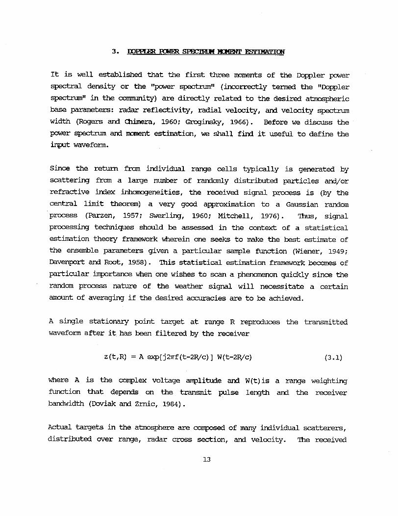
It is well established that the first three moments of the Doppler power
spectral density or the "power spectrum" (incorrectly termed the "Doppler
spectrum" in the community) are directly related to the desired atmospheric
base parameters: radar reflectivity, radial velocity, and velocity spectrum
width (Rogers and Chimera, 1960; Groginsky, 1966). Before we discuss the
power spectrum and moment estimation, we shall find it useful to define the
input waveform.
Since the return from individual range cells typically is generated by
scattering from a large number of randomly distributed particles and/or
refractive index inhomogeneities, the received signal process is (by the
central limit theorem) a very good approximation to a Gaussian random
process (Parzen, 1957; Swerling, 1960; Mitchell, 1976). Thus, signal
processing techniques should be assessed in the context of a statistical
estimation theory framework wherein one seeks to make the best estimate of
the ensemble parameters given a particular sample function (Wiener, 1949;
Davenport and Root, 1958). This statistical estimation framework becomes of
particular importance when one wishes to scan a phenomenon quickly since the
random process nature of the weather signal will necessitate a certain
amount of averaging if the desired accuracies are to be achieved.
A single stationary point target at range R reproduces the transmitted
waveform after it has been filtered by the receiver
z(t,R) = A exp[j2rf(t-2R/c) W(t-2t-2R/c) (3.1)
where A is the complex voltage amplitude and W(t)is a range weighting
function that depends on the transmit pulse length and the receiver
bandwidth (Doviak and Zrnic, 1984).
Actual targets in the atmosphere are composed of many individual scatterers,
distributed over range, radar cross section, and velocity. The received
13
waveform for a particular distributed target then is a sample function of
the random process which produces the atmospheric return. We desire to
estimate the mean characteristics of the random target over an ensemble of
sample functions. The vector sum of the return complex voltage from the
individual scatterers is
z(t,R) = Z Ai exp[j2fi(t-2Ri/c)] W(t-t2Ri/c) (3.2)i
where the subscript i represents the individual particle. Each particle has
a complex voltage return (Ai), a Doppler shifted frequency (fi), and a range
(Ri). At any given sampling instant for the kth pulse the received waveform
can be represented in the complex signal plane by a vector (or "phasor")
which has an instantaneous amplitude or voltage IVk(R) and phase Ek(R)
determined by the instantaneous vector sum of the individual scatterers.
The complex signal is then
Zk(R) = Ik(R) + j Qk(R) (3.3)
where Ik(R)=IVk(R) Icos ek(R) is the in-phase and Qk(R)=|Vk(R) Isin Ek(R) is
the quadrature phase component (Rader, 1984). These expressions illustrate
that (for a specific received polarization) only two quantities are
measurable, the complex amplitude and phase. All other quantities are
derived from these based on physical models.
3.1 GENERAL FEURES OF THE DOFPPER POWER SECRM
The concept of the Doppler power spectrum is fundamental in radar signal
processing (Haykin, 1985b). A typical power spectrum, shown in Figure 3.1,is a plot of the returned power as a function of the Doppler shifted
frequency components in the target resolution volume. The usual sign
convention (taken from spherical coordinates) is that a positive Doppler
velocity corresponds to a velocity away from the radar; the rate of change
in range is positive. This corresponds to a negative Doppler frequency
shift. The velocity limits ±Vmax are determined by the Nyquist constraint
that two samples per wavelength or period are required to unambiguously
measure a frequency (Whittaker, 1915; Nyquist, 1928; Shannon, 1949). For a
14

0
-10
dB -20
-30
-40-0.5 -0.4 -0.3 -0.2 -0.1
VELO
Fig 3.1 Doppler power spectrumecho in white noise.Vmax, velocity spectrum
0 0.1 0.2 0.3 0.4 0.5)CITY/2 Vmax
(128 point periodogram) of typical weatherEstimated parameters are velocity 0.4width ~ .04 Vax, and SNR ~ 10 dB.
15

uniform pulse repetition time Ts (equally spaced samples) the so called
"Nyquist velocity" is
Vmax = \/4Ts . (3.4)
The interval [-Vmax, +Vma] is called the "unambiguous velocity interval" or
commonly the "Nyquist velocity interval" and all possible velocities are
measured within this interval. The reality of sampling theory dictates that
sampled Doppler spectra exist on a circular frequency domain rather than a
frequency line extending both directions from zero (Gold and Rader, 1969).
Thus, as a target velocity increases beyond Vmax, it aliases or "folds" onto
the negative velocity region of the Nyquist velocity interval (Passarelli,
et al., 1984).
The signal power spectrum rests on a platform of "white noise", so called
because the noise power spectral density is independent of frequency. White
noise is caused by several factors including thermal noise from the
receiver, phase noise from the transmitter/receiver system, artifacts from
the spectrum estimation algorithm, artifacts from receiver non-linearities,
and quantization noise from the A/D converters.
It is convenient to approximate the signal portion of the power spectrum
with a Gaussian shape having some mean velocity and width. The area under
the signal portion of the spectrum, not including the contribution of white
noise, is the returned power. Depending on the distribution of velocities
in the pulse volume and the scattering mechanism, asymmetric spectra and/or
multi-modal spectra may occur. Second trip echoes are a common cause of
bimodal spectra in klystron systems. Janssen and Van der Spek (1985) found
that only about 75% of observed precipitation spectra had the assumed
Gaussian shape.
For ST/MST radars the spectrum is often assumed to be Gaussian, but spectra
measured at near vertical antenna beam directions (zenith angles less than
about 10°) very regularly show one or more strong spectral spikes superposed
on a Gaussian shaped base. The spikes result from a corresponding number of
16

quasi-horizontal laminar refractive index structures producing partial
reflections while the Gaussian floor results from scattering by turbulent
refractive index structures. Moreover, the aspect sensitivity due to the
quasi-horizontal laminar structures may produce strongly asymmetric mean
power spectra if several single power spectra are averaged for oblique
antenna beam directions.
The width of the velocity spectrum has a number of contributions including
wind shear, turbulence, particle fallspeed dispersion, antenna rotation
(Nathanson, 1969) and, in the case of lidar, range propagation of the pulse
during sarpling. It is difficult to separate instrumental effects from the
desired signal contributions.
The goal of signal processing is to deduce the characteristics of the signal
portion of the spectrum. This means that the other contributions from
clutter, noise, and artifacts must be either minimized or removed by the
various steps of processing. There are two basic approaches: frequency
domain processing using the power spectrum, and time domain processing using
the autocorrelation function. Each approach has its advantages and
disadvantages but the essential information available from each is identical
since the power spectrum of the sampled signal and its autocorrelation
function comprise a Discrete Fourier Transform (DFT) pair, (Oppenheim &
Schafer, 1975; Tretter, 1976):
N-1S(nfo) = Z R(mTs) exp [-j2mnm/N] (3.5a)
m=0
N-lR(miTs) = N- 1 Z S(nfo) exp [+j27rmn/N] (3.5b)
n=0
where S(nfo) is the Doppler spectrum in multiples of the fundamental
frequency shift fo=l/NTs and R(rTs) is the autocorrelation function in
multiples of the sample time Ts. This is the discrete version of the
celebrated Wiener-Khinchine theorem (Wiener, 1930; Khinchine, 1934). The
information content is identical in the two approaches. The primary
difference between time and frequency domain processing is that the
17

information concerning the lower spectral moments is distributed over
several frequencies of the power spectrum, while it is concentrated in the
small lags of the autocorrelation function.
It is important to realize that sampling theory dictates that both S(nfo)
and R(mrs) be periodic. That is, the spectrum repeats at multiples of the
sampling frequency and the correlation function repeats at multiples of N
times the sampling period (NTS). When highly coherent spectral components
(e.g. clutter) are present, the correlation usually will not decay to zero
within the N/2 samples. Thus, the periodicity requirement of R(mTs) will
produce a biased spectrum estimate. Care must be exercised in these cases.
3.2 FREQUENCY DOMAIN SPECTRAL MEMENT ESTIMATION
Estimating the Doppler power spectrum and its moments directly are
straightforward techniques (Haykin and Cadzow, 1982). However, some basic
questions must be answered first. We implicitly assume a data model for
weather and clutter spectra when we choose a spectrum estimation technique.
A specific data model such as a sum of sinusoids or white noise passed
through a narrowband filter is best analyzed by a spectrum analysis
technique compatible with that data model. Robinson (1982) emphasizes this
point in his historical review of spectrum estimation. Marple (1987)
stresses the importance of using an appropriate model fitting analysis and
gives a very well organized discussion of classical and modern spectral
estimates using digital techniques.
3.2.1 Fast Fburier transform techniques
The Doppler power spectrum may be estimated from the Discrete Fourier
Transform (DFT) of the complex signal. The DFT decomposes the observed data
into a sum of sinusoids having amplitude and phase that will exactly
reproduce the observed data. It is easy to show that these N discrete
components are adequate to reconstruct the entire continuous spectrum so
long as the complex data samples {zk} are taken at a rate equal to or
greater than the bandwidth of the signal. The advantage of measuring the
full Doppler spectrum is that spectral impurities such as ground clutter,
18

bi-modal spectra or artifacts can be suppressed by intuitive (if non-
optimal) algorithms.
The so called "periodogram", a frequently used estimator in weather radar as
well as many other fields, is an N point spectrum estimator in which the
standard deviation of each spectral value equals its mean value. Usually
one averages several spectra from a divided time series or smooths over
several points in the periodogram to improve the accuracy. The periodogram
is defined as the squared magnitude of the transformed data sequence {Zk}
(Blackman and Tukey, 1958; Cooley and Tukey, 1965; Oppenheim and Schafer,
1975),
N-1P(f) = N-11 Z hkzk exp [-j27fk]1 2 (3.6)
k=-O
where the """ denotes an estimate. The hk term is the "window" which
modifies the waveform being transformed.
In general, window functions have a maximum value centered on the time
series and are tapered near zero at the ends. This tapering reduces the
spectrum smearing, a "leakage" of spectral energy introduced by the
discontinuity imposed by sampling when the end points are joined. Windowing
also effectively reduces the number of points in the time series. The
simplest window is hk = 1 (or no windowing). For this window, the
periodogram of a single point target has the first side lobe only 13 dB down
from the peak. This is not a problem for estimating the mean and variance
of the designed signal, but if strong clutter is present, then the sidelobe
power from the clutter that leaks throughout the Nyquist interval can mask
weaker weather echoes. Table 2 shows characteristics of several common
windows. Harris (1978) and Marple (1987) both give an extraordinary
description of window functions. In general, the lower the sidelobes
offered by a window, the broader its main lobe response. This broadening
degrades the spectral moment estimates.
19

Table 2
Characteristics of time series data windows (Marple, 1987).
Equivalent 1/2 PowerWindow Highest Sidelobe Bandwidth Bandwidth
Name Sidelobe Decay Rate (Bins) (Bins)
Rectangle -13.3 dB -6 dB/octave 1.00 0.89Triangle -26.5 dB -12 dB/octave 1.33 1.28Hann -31.5 dB -18 dB/octave 1.50 1.44Hamming -43 dB -6 dB/octave 1.36 1.30Gaussian -42 dB -6 dB/octave 1.39 1.33Equiripple -50 dB 0 dB/octave 1.39 1.33
The windowed periodogram P(f) can be evaluated at any frequency f in the
Nyquist interval. The Fast Fourier Transform (FFT) is simply a highly
efficient technique for evaluating the DFT at N equally spaced discrete
frequencies (Welch, 1967). Although the FFT algorithm is attributed to
Cooley and Tukey (1965), a recent historical investigation into the history
of the Fast Fourier Transform by Heideman, et al. (1984) attributes an
algorithm very similar to the FFT for computation of the coefficients of a
finite Fourier series to Gauss, the German mathematician. Apparently the
first implementation of the FFT on a weather radar was in December 1970 at
the CHILL radar (Mueller and Silha, 1978).
3.2.2 Maximum entrpy techniques
The aforementioned Fourier transform techniques have been understood since
the time of Fourier and Gauss and are well documented by Jenkins and Watts
(1968). Only recently have techniques based on covariance estimates and
probabilistic concepts been explored. Kay and Marple (1981) and Childers
(1978) have termed these parametric techniques "modern spectrum analysis".
Marple (1987) points out that maximum entropy, maximum likelihood and other
techniques are "modern" in the sense that short data sequences produce
spectral resolutions better than the inverse duration of the data sequence,
which is characteristic of classical spectrum estimators. Furthermore, fast
digital algorithms have been developed which allow computing hardware to
perform the computations in the required time frames. This interest in
20

alternative spectrum estimators can be explained by categorizing expected
performance improvements as increased resolution or increased detectability.Both Jaynes (1982) and Makhoul (1986) attempt to clarify some confusion and
misleading notions related to the maximum entropy techniques.
Maximum entropy (ME) spectrum analysis estimates the spectrum using
parametric techniques to define the spectrum. The parameters are typically
derived from the data samples or some estimated autocorrelation sequence.
The ME technique was developed by J.P. Burg (1967, 1968, 1975) as a
geophysical prospecting technique for high resolution measurement of sonic
wave reflections and velocities. Makhoul (1975) shows that the all pole ME
spectrum model can approximate any spectrum arbitrarily closely by
increasing its order L. He shows that the ME spectra minimizes the log
ratio of the estimated spectrum to the true spectrum integrated over the
Nyquist interval. The MST radar community (Klostermeyer, 1986) and the
lidar community (Keeler and Lee, 1978) have used the maximum entropy method
for characterizing atmospheric targets. Sweezy (1978) and Mahapatra and
Zrnic (1983) have computed maximum entropy spectrum estimates on simulated
weather radar data and compared them with Fourier transform and pulse pair
estimators. Haykin, et al. (1982) describe how maximum entropy techniques
can be applied to Doppler processing of radar "clutter" including weather
and birds for aviation hazard identification.
Atmospheric echoes, whether from precipitation, aerosols, or turbulence, can
be modeled by "autoregressive" (AR) techniques as narrow band filtered
noise. These AR and the standard Fourier technique appear to represent the
essential spectral features well although little quantitative work is
available for comparison in the atmospheric echo application. Van den Bos
(1971) and Ulrych and Bishop (1975) show that maximum entropy spectrum
analysis is equivalent to least squares fitting of a discrete time all pole
model to the observed data. As noise is added to the observations the
autoregressive moving average (ARMA) model is more appropriate (Cadzow,
1980; Marple, 1987).
21

The justification for studying maximum entropy spectra is its ability to
estimate complete spectra from the first few lags of the autocorrelation
function rather than from all the autocorrelation lags that are required by
the Fourier transform technique (Radoski, et al., 1975). Since only the
first few autocorrelation values are known with any confidence, this
property may be critically important when the sampled data sets are very
short. Baggeroer (1976) computes confidence limits for ME spectra which are
applicable to atmospheric echoes.
The "order" of the maximum entropy spectra defines the number of lags, or
equivalently the number of poles in the filter through which white noise is
passed in modeling the data. A larger order allows non-Gaussian spectral
detail to be more accurately represented, e.g. a weak atmospheric echo in
the presence of a much stronger ground clutter. However, a larger order
requires a longer data sample to obtain accurate estimates.
The basic technique uses the sampled input data to compute R(0), R(1),...
R(L) for the Lth order estimator. Additional lags are realized by requiring
that the entropy (in an information theoretic sense) of the probability
density function having the extended autocorrelation function be maximized.
This extended autocorrelation function allows computation of coefficients
for a whitening or linear prediction filter. The ME spectrum is computed
from these filter coefficients which are defined by the matrix equation
A = R-1P (3.7)
where A is the filter coefficient vector, R is the autocorrelation matrix
and P is the autocorrelation vector (Ulrych and Bishop, 1975). The
coefficient estimates can be rapidly computed using the Levinson algorithm
(Makhoul, 1975; Anderson, 1978).
This filter removes the predictable components from the input data and the
optimum filter of order L minimizes the prediction error. The Lth order ME
spectrum estimate can then be computed
22

^2 (L)
SME (f) (3.8)L
I1 -e am exp[-j2rfm] 12
m=l
where am are the elements of A and ao2(L) is final prediction error. Burg
(1967) gives the "forward-backward" technique of estimating the linear
prediction coefficients directly from the data which frequently permits more
detail to be shown in the spectrum. Smylie, et al. (1973) and Haykin and
Kesler (1976) give the complex form of the ME spectrum estimator.
Friedlander (1982) and Makhoul (1977) describe lattice structures for ME
spectrum estimates which are computationally more efficient and identical toBurg's method. Papoulis (1981) attempts to interrelate the various aspects
of maximum entropy and spectrum estimation in his mathematical review paper.
Marple (1987) presents a more readable exposition. Cadzow (1980, 1982)
extends the ME concept to rational models.
Keeler and Lee (1978) and Mahapatra and Zrnic (1983) have shown that the
pulse pair frequency estimator is identically the mean (or the peak, in this
special case) of the first order maximum entropy spectrum. The atmospheric
remote sensing community has been using the simplest form of ME for almost
two decades! Its relevance to accurate parameter estimation for weather
radars, ST/MST profilers and lidar signals is an active research area
(Haykin, 1982).
3.2.3 Maximum likelihood techniques
Maximum likelihood (ML) estimation is a statistical concept that gives the
most likely outcome or minimum variance estimate of an experiment based on a
set of known probabilities. ML estimates of spectral parameters are
"efficient", i.e. there is no other unbiased estimator having a lower
variance. It is well suited for estimating parameters of a spectrum whose
shape is known or assumed when neither a priori knowledge nor a valid cost
function associated with moment estimator error is known (Van Trees, 1968).
Zrnic (1979a) uses ML techniques to derive the minimum variance (Cramer-Rao)
23
bounds of spectral moment estimators for application to atmospheric radar
data. He compares present estimators to these bounds and interprets Levin's
(1965) results in a modern framework. Moreover, he shows that the pulse
pair estimator is ML for a Markov process.
In general closed form solutions for ML estimates of spectrum moments are
quite complicated and difficult to compute. The optimum (ML) processor
depends on the underlying signal statistics which in turn depend on the
spectrum shape and SNR. Shirakawa and Zrnic (1983) evaluate the ML
estimator for sinusoids in noise and find a slight improvement over the
pulse pair estimator at low SNR's. Novak and Lindgren (1982) derive the
exact ML mean velocity estimator for Gaussian shaped spectra using more than
one autocorrelation lag. Their technique is similar to Lee and Lee's (1980)
poly pulse pair velocity estimator. Miller and Rochwarger (1972) show that
for independent pairs, the pulse pair estimator of mean frequency is ML for
an arbitrarily shaped spectrum so long as the normalized width is small.
Sato and Woodman (1982) use a least square fit algorithm to estimate
spectral parameters, including noise and clutter parameters, by assuming
prior knowledge of the spectral shapes. Woodman (1985) shows that this
technique is a ML estimator of the spectral characteristics. It is
gratifying that the simple pulse pair estimators approach the minimum
variance bound over a wide range of SNR's.
If the spectrum shape is completely unknown, the ML spectrum gives the most
probable estimate which concentrates the spectral energy at the input signal
frequencies while minimizing other spectral energy in a statistically
optimum sense (Capon, 1969; Lacoss, 1971). The statistical rationale for
using ML estimation is that the ML spectrum estimate provides a minimum
variance, unbiased estimate of the power at a given frequency. Burg (1972)
has shown that in the mean the Lth order ML spectrum is just the following
combination of ME spectra up to order L:
L[SML(f) - 1 = L1 Z [SME,m(f)- 1 (3.9)
m=l
24

Thus, the mean ML spectrum is a smoothed version of mean ME spectra. It has
many of the same properties as ME spectra but the details are obscured by
combining all order ME spectra. There have been theoretical studies of ML
spectra but little application to atmospheric data. Klostermeyer (1986) has
computed ML spectra for VHF radar data.
3.2.4 Classical spectral moment computation
The spectrum moments can be directly related to the reflectivity, velocity,
and dispersion parameters desired for further analysis. Computing these
moments has historically been performed using classical moment calculations
based on techniques from probability theory when considering the power
spectrum as a density function of frequency or velocity components of the
desired signal (Denenberg, 1971, 1976). For sampled data systems the
"sampling theorem" imposes certain requirements on moment and transform
computations that cannot be ignored -- namely replication in the frequency
domain and circular convolution (Oppenheim and Schafer, 1975).
Let the power spectrum of the received signal be denoted by S(f). Then the
classical spectral moments are given by
Mn = x fn S(f)df . (3.10)
The zeroth moment (MO) is the area under S(f) and represents total signal
clutter, and noise power. Of course, we are usually interested only in the
signal power, so the clutter and noise powers must be estimated and removed.
Noise power is generally easy to remove, but clutter removal causes
difficulties to the parameter estimation process.
The classical normalized first moment represents mean velocity and is given
by the linear weighting of S(f) over the Nyquist interval
fc = f S(f)df / Mo (3.11a)
V = (X/2) fc (3. 1Ib)
25

Note that white noise biases the velocity towards zero and for a pure noise
spectrum the mean velocity is identically zero. Various techniques have
been described for mitigating this bias, most of them requiring manipulation
of the power spectra. Thresholding the spectrum points with some value near
the noise spectral density is common, but some sensitivity is lost
(Hildebrand and Sekhon, 1974; Sirmans and Bumgarner, 1975a; Klostermeyer,
1986).
The "spectral balancing technique" rotates S(f) until the signal spectrum is
near zero so that the signal and the noise share the same zero mean
velocity. The amount of rotation represents the mean velocity of the signal
component and removes errors due to aliased spectra. The same effect is
obtained by computing the offset first moment
4 (f-fc) S(f)df = 0 (3.12)
where fc is varied to obtain equality.
The normalized second central moment represents the velocity dispersion
within the pulse resolution volume. Shear, turbulence and precipitation
motion (fallspeed oscillations, etc.) contribute to a distribution of radial
velocities (Nathanson and Reilly, 1968). A contribution from antenna
scanning during the finite dwell time may also be significant (Nathanson,
1969). The velocity dispersion (width) is the square root of the second
central moment of the spectrum estimate:
af2 = I (f-fc)2 S(f)df / M0 (3.13a)
W = (>/2) of . (3.13b)
Spectrum estimation algorithms are fairly time consuming to invoke, and once
the frequency domain is entered, there is still substantial computation to
accurately extract the meteorological moments. The main reason for entering
the frequency domain lies in the ability to more easily filter spectral
26

artifacts or identify multi-modal spectra. In cases where spectra are
unimodal and generally free from artifacts, more efficient time domain
processing is typically used.
3.3 TIME DIXMAIN SPECTRAL MO'ENT ESTIMATIC
The basis for time domain moment estimation is the transform relationship of
the autocorrelation function of the complex signal to the power spectrum.
An estimate of the autocorrelation can be easily calculated from the complex
input time series {Zk),
N-m-1R(m) = (N-m) 1 2 Zk* Zk+m (3.14)
k=0
where m is the lag between the two data series. For uncontaminated spectra,
usually only two or three lags are necessary to obtain the moments of
interest. This represents a substantial savings in computation over the
spectrum domain approach. The general relationship between the complex
autocorrelation function and the nth classical spectral moment is
Mn = R[n](0)/(j2w)n (3.15)
where R[n] (0) is the nth derivative of the autocorrelation function
evaluated at lag = 0 (Papoulis, 1962; Bracewell, 1965). The first three
spectral moments are used to estimate the reflectivity, radial velocity, and
velocity dispersion or width respectively (Miller, 1970; Miller, 1972).
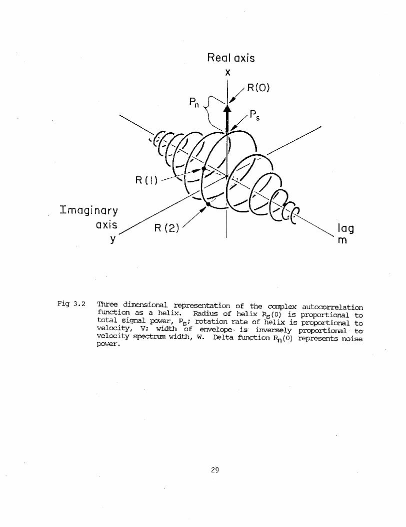
3.3.1 Gecmetric interpretatins
The complex autocorrelation function, which is the basis for time domain
moment estimation, is often depicted as its real and imaginary components,
but an alternative 3 dimensional representation allows a better
understanding of the covariance, or pulse pair, mean frequency estimator.
Consider the complex R(m) to be a 3D helix that is wide at the center and
tapered toward zero radius at the ends having a Gaussian shaped envelope.
27

Figure 3.2 shows a drawing of this continuous autocorrelation helix. A
sampled autocorrelation helix will consist of points on this helix spaced at
the PRT. Note that zero lag, R(0), is at the center and has no imaginary
component. The radius at lag 0 represents the signal power and the real
delta function at lag 0 represents the noise power. The width of the
Gaussian envelope of the helix represents the inverse velocity spectrum
width or dispersion. The rotation rate of the helix defines the mean
velocity of the signal. For a given spacing of autocorrelation function
samples the angular rotation between a pair of samples is a measure of mean
velocity. Thus, the angle of the complex estimate R(1) gives the mean
velocity of the received signal expressed as a fraction of the Nyquist
interval which is the "pulse pair estimator" used almost universally for
mean velocity in weather radar and lidar processors.
A useful geometric interpretation of the relationship between classical
spectral moments and the autocorrelation function can be found in Passarelli
and Siggia (1983). This interpretation illustrates many of the properties
of pulse pair estimators.
3.3.2 "Pulse pair" estimators
The advent of the so-called pulse pair, double pulse, or complex covariance
technique (Rummler, 1968a; Woodman and Hagfors, 1969; Miller and Rochwarger,
1972; Berger and Groginsky, 1973; Woodman and Guillen, 1974) for mean
velocity estimation was revolutionary since the algorithm arose at about the
same time that it could be implemented in hardware for a significant number
of range bins. Lhermitte (1972) and Groginsky (1972) reported the first use
of hardware signal processors and weather radars using this technique.
However, covariance processing for velocity measurements apparently was
first used in March of 1968 for ionospheric velocity measurements (Woodman
and Hagfors, 1969). Woodman and Guillen (1974) also reported covariance
based velocity measurements in the mesosphere at the Jicamarca MST radar in
1970. This algorithm development in the MST community was independent of
Rummler's work. The pulse pair algorithm led to an exciting growth in the
use of Doppler radar by the scientific community (Groginsky, et al., 1972;
Ihennitte, 1972; Sirmans, 1975; Ihermitte and Serafin, 1984).
28
Real axisx
Pn
R(I)
Imaginaryaxis
v1J
Fig 3.2 Three dimensional representation of the complex autocorrelationfunction as a helix. Radius of helix Rs(O) is proportional tototal signal power, Ps; rotation rate of helix is proportional tovelocity, V; width of envelope! is inversely proportional tovelocity spectrum width, W. Delta function Rn(0) represents noisepower.
29
R(O)
PS
lagm

Other time domain algorithms such as the "vector phase change" (Hyde and
Perry, 1958) and the "scalar phase change" (Sirmans and Doviak, 1973) are
closely related to the pulse pair estimator, but their performance is
inferior. Sirmans and Bumgarner (1975b) capare these and other mean
frequency estimators.
It is well known that the first few lags of the autocorrelation function are
sufficient to deduce spectrum parameters of interest. Papoulis (1965 and
1984), Bracewell (1965), Woodman and Guillen (1974), and Passarelli and
Siggia (1983) show that the autocorrelation function can be represented by a
Taylor series expansion in terms of the central moments of the Doppler
spectrum with the low order moments being the leading terms. In other
words, the first few lags of the autocorrelation function contain the moment
information of interest. For an arbitrary spectrum, these expansions have
the form
R(mits) = A(mrTs) exp[-j0(mrs)] . (3.16)
The even function A(mrTs) is determined primarily by the even central moments
(e.g., power, variance and kurtosis), while the odd function 0(mTs) is
determined primarily by the mean velocity and the odd central moments (e.g.,
skewness).
Estimators can be generated for any moment, provided that a sufficient
number of autocorrelation lags are measured. White noise power Pn biases
the magnitude for lag zero. Therefore, the total received power must be
corrected for noise,
Pr = R(0) - Pn (3.17)
The pulse pair mean velocity estimator is not biased by white noise and is
obtained by taking the argument of the first autocorrelation lag,
V = ( /2) (2Ts)-1 tan[Im R(T)/Re R(Ts)] . (3.18)
30

The pulse pair spectrum width is given by
W = ( X/2) (2fTs)- 1 [1 - p(Ts) (1 + SNR-1)] (3.19)
where p(Ts) =|R(Ts) |/R(O) is the normalized first lag and the noise power
must be determined independently.
3.3.3 Circular spectral rmment computation for sampled data
Sampled data systems utilize the complex plane and z-transform theory to
formally express the relationships between the time and frequency domains
(Oppenheim and Schafer, 1975). For example, the DFT of the autocorrelation
function is formally the z-transform of the sampled autocorrelation function
evaluated on the unit circle in the z plane, i.e. |z|=1 or z = exp[-j27f]:
N-1S(f) = z R(mTs) z-m (3.20)
m=O I z=exp [-j 27rf]
The unit circle on the complex z plane is important in understanding
concepts of sampled or discrete data systems, specifically concepts of
digital signal processing. Figure 3.3 shows the z plane and the frequencies
associated with various points on the unit circle. Zero frequency, where
ground clutter usually appears, corresponds to z=l and the Nyquist frequency
(where velocity spectra alias into the next Nyquist velocity interval)
corresponds to z=-l. Thus, the z plane representation of spectral space
allows an immediate and simple geometric interpretation of velocity aliasing
and the velocity ambiguity arising from sampling too slowly. Analysis and
synthesis of digital filters requires heavy application of z transform
theory, thus easily allowing visualizing the effect of various types of
ground clutter filters, for example.
It is natural to compute spectral moments on the unit circle rather than
along the frequency line in the Nyquist velocity interval. The zeroth
moment or total receiver power, is still that area under the spectrum
31

Imag
f = (2Ts)-'
Real
I0
f = -(4Ts )-I Z plane
Fig 3.3 Periodogram power spectrum plotted on unit circle in the z-plane.Note velocity aliasing point, the Nyquist velocity, at z=-l.
32
whether on a line or on a circle. However, higher order moments can be
different for the two cases (Passarelli, et al., 1984).
A simple geometric derivation shows that the first circular moment estimate,
fc, of the estimated spectrum, S(f), is the normalized frequency at which
the center of mass on the circle is located,
S (27m/N) sin(27m/N)fc = (27)- 1 tan-1 (3.21)
Z S(27m/N) cos(2nm/N)
where the summations run over 0 to N-l. Trigonometric manipulation converts
this equation to
N-1Z S(27m/N) sin[27(n/N - fc)] = 0 . (3.22)
n=0
Thus, fc is the sinusoidal weighted mean of S(f) (Zrnic, 1979a). Further,
we see that the numerator and denominator of (3.21) are the imaginary and
real parts of R(mrTs) and that the circular first moment is identically the
pulse pair frequency or velocity estimator.
Two points are clear from this discussion: 1) white noise does not bias the
pulse pair frequency estimate because the noise does not weight any
particular frequencies on the circle, and 2) symmetric spectra have
identical first moments using either the classical (linear weighting) or the
circular (sinusoidal weighting) computations. Asymmetric spectra produce
different first moment estimators but there are no compelling reasons to
prefer linear weighting over the more common sinusoidal weighting (the pulse
pair estimator). Indeed, for sampled data systems the circular moment
computation is more natural than classical moment computation.
3.3.4 Pbly pulse pair techniques
If we accept the premise that knowing lags of the autocorrelation function
past the first allows a processor to extract additional information about
the received signal, then one should expect to reduce the variance of
velocity estimates by using, not only R(1), but R(2), R(3), etc. The
33
Classical:
2(f - f,,i) S(f)= o
2Ts freq - Y 2Ts
Circular:
Zsin[27r (f fci)]S(f) 0-t~~~~~i,,]scr, ·o~~~~~~~~~~~~
fcir +2T5
Fig 3.4 Comparison of classical and circular (pulse pair) first momentestimators. Classical estimate is determined by linear weightingof spectrum estimate and circular estimate, by sinusoidalweighting.
34
m
m

variance reduction can be realized only if the received signal is coherent
over the additional lags. Lee (1978) proposed the "poly pulse pair"
algorithm for lidar signal processing. Velocity estimates can be found from
a weighted average of the estimate given at each lag, where the smaller lags
are given higher weighting since the correlations are higher. Poly pulse
pair velocity estimates (using a few lags) produce lower variance estimates
than the pulse pair estimates when the spectrum width of the signal is only
a few percent of the sampling frequency (Lee and Lee, 1980).
Strauch, et al. (1977) evaluated poly pulse pair for 3 cm radar processing.
They concluded that for typical velocity spectrum widths and PRF's (sample
rates) used with X-band Doppler radar, the coherence time was frequently too
short to give a significant improvement in the velocity estimates. However,
for infrared lidar the coherence times and sample rates permit a significant
improvement in reflectivity, velocity, and width estimates (Bilbro, et al.,
1984). Furthermore, Rastogi and Woodman (1974) and Srivastiva, et al.
(1979) use multiple lag estimates of the correlation function to estimate
moments of a Gaussian shaped spectrum. Several independent estimates of the
autocorrelation function can be found and a Gaussian shaped curve fitted to
these samples. Sato and Woodman (1982) have used this nonlinear curve
fitting technique to estimate signal, clutter, and noise parameters at the
Arecibo ST radar.
3.4 UNCERTAINTIES IN SPECThUM UMENT ESTIfM4AI
Any estimator has an associated uncertainty. In atmospheric radar signal
processing the velocity spectrum moments are being estimated with some
uncertainty that depends on the processing interval, the coherence time or
velocity width, and the SNR. Zrnic has published extensively on weather
radar spectrum estimator uncertainties and his results are succinctly
described in Doviak and Zrnic (1984). A summary is given here.
3.4.1 Reflectivity
Marshall and Hitschfeld (1953) describe the probability density function of
the distributed weather target. The received signal is a complex Gaussian
process which has a Rayleigh amplitude distribution and an exponential power
35

distribution. Thus, the mean received signal power is Ps with variance Ps2
and the coherence time is determined by the spectrum width of the signal.
The number of independent signal samples in a given integration time Td
seconds is approximately MI = 2/WTd (Doviak and Zric, 1984) where W is the
spectrum width (standard deviation) in Hertz. The number of independent
noise samples is just M = Td/Ts, the total number of samples in the dwell
time. Therefore, the variance of the mean power estimate is approximately
var(Pr) = Ps2/MI + Pn2/M . (3.23)
Doviak and Zrnic (1984) show that if the number of independent signal
samples is smaller than about 20 and a log receiver is used, the bias in the
estimated received power depends on MI and its variance is not exactly
proportional to 1/MI. A square law receiver does not encounter these
problems. Marshall and Hitschfeld (1953), as well as a recent review by
Ulaby, et al. (1982), show that the ratio of the mean power to the
fluctuating power associated with a single sample of a Rayleigh quantity is
5.6 dB. Therefore, for MI independent samples the signal power estimates
are known within 5.6/MjI dB. Averaging independent samples obtained in
range can further reduce the variance.
3.4.2 Velocity
Woodman and Hagfors (1969) used statistical analysis of Gaussian random
variables to estimate the uncertainty of pulse pair velocities. Berger and
Groginsky (1973) applied perturbation analysis to derive the variance of the
independent and contiguous pulse pair frequency estimators. Zrnic (1977b)
later extended their results to spaced but correlated pulse pairs. Two
conditions, both of which are usually satisfied for a large number of
samples (M), are necessary for the analysis to be accurate:
M >> A /47 W Ts (3.24a)
M >> (SNR-1 + 1)2 / p2(Ts) (3.24b)
where W is the velocity spectrum width and p(Ts) = R(Ts)/R(0) is the
autocorrelation function at lag Ts (the PRT) normalized to unity. At high
36

SNR and for large enough M that both conditions are satisfied, and for
contiguous pairs typical of radar Doppler processing, and for Gaussian
shaped spectra, the variance of the velocity estimate is
var(V) = f W/ 8/7 M Ts . (3.25)
Table 3 summarizes the velocity uncertainties at high SNR for three cases:
1) contiguous samples, 2) independent sample pairs, and 3) the minimum
variance bound. Expressions are given both in terms of the actual spectrum
width in ms -1 (W) and the width normalized to the Nyquist velocity interval
(Wn). Figure 3.5 shows the standard deviation of velocity estimates
normalized to the Nyquist velocity interval and to the square root of the
number of samples M as a function of the normalized spectrum width. The SNR
is a parameter for the two sets of curves -- those for the typical
contiguous pairs and for less typical spaced pairs of pulses (Campbell andStrauch, 1976; Doviak and Zrnic, 1984). Note that reasonably accurate
velocity estimates can be obtained for a given M doawn to SNR ~ 0 dB so long
as the Gaussian standard deviation velocity width is less than about 0.2 of
the Nyquist velocity interval 2Vmax.
Woodman (1985) discusses errors for multiple lag velocity estimators in
which the lags are statistically dependent. By weighting the correlation
estimates in an optimum fashion, he concludes that for high SNR only a few
(2 or 3) lags are necessary.
3.4.3 Velocity spectrum width
Benham, et al. (1972) and Berger and Groginsky (1973) applied a perturbation
analysis to the spectrum width estimator and Zrnic (1977b) later extended
their results to arbitrarily spaced pulse pairs. Their primary result for
high SNR, contiguous pairs, and narrow, Gaussian shaped spectra is that the
variance of the velocity width is
var(W) = 3 XW / 64/T M Ts . (3.26)
37

THBLE 3
Expressions for variance of velocity estimators at high SNR. AssumesGaussian spectra in white noise, low normalized velocity width (Wn=W/2Vmax)and large M. Expressions apply to both pulse pair and Fourier transformestimators.
Var(V) using W
Contiguoussamples(typical case)
x8]/7w MT
Independentpairs
2M
Minirumvariancebound
48 TS2
-MX2 W4M X2
Var(V) using Wn
W wn167r MTs 2
X2Wn2
8Mr 25
3 \ 2
Wn4
MTs2
38
C\M
Q<>
( '°V 1.0
z0
u 0.5Q0
Q0 0.1 0.2 0.3 0.4
NORMALIZED SPECTRUM WIDTH oavn
Fig 3.5 Velocity error as function of spectrum width and SNR. Spectrumwidth is normalized to Nyquist interval, vn=W/2Vn1 =2WTs/X. M isnumber of sample pairs and error is normalized to Nyquist velocityinterval, 2va = 2Vmax . Small circles represent simulation values(Doviak and Zrnic, 1984).
39

Table 4 summarizes the width uncertainties at high SNR for three cases: 1)
contiguous samples, 2) independent sample pairs, and 3) the minimum variance
bound. Expressions are given both in terms of the actual spectrum width in ms-1
(W) and normalized to the Nyquist velocity interval (Wn). Figure 3.6 shows the
normalized standard deviations of the width estimates as a function of normalized
spectrum width for a range of SNR's. The width estimator is relatively good ifthe normalized width is between 0.02 and 0.20 of the Nyquist interval and the SNR> 5 dB.
40

TABLE 4
Expressions for variance of width estimators at high SNR. Assumes Gaussianspectra in white noise, low normalized velocity width (Wn=W/2Vmax) and large M.Expressions apply to both pulse pair and Fourier transform estimators.
Var(W) using W Var(W) using wn
Contiguoussamples(typical case)
3w
64W,/642z MTs
3 X2
Wn128J7r MTS 2
Independentpairs
Minimumvariancebound
w2
2M
x 2 28MT2 Wn2
8MTs281]?
2880 T 44 W6
M X4
45 X2
MTS2
41

c
0
C
0.5az
cn n0 . 1 0.2 0.3 0.4
NORMALIZED SPECTRUM WIDTH, Ovn
Fig 3.6 Width error as a function of spectrum width and SNR. Spectrumwidth is normalized to Nyquist interval, vn=W/2Vmax=2WTs/X- M isnumber of sample pairs and error is normalized to Nyquistinterval, 2Vmax . Small circles represent simulation values(Doviak and Zrnic, 1984).
42
I
I

4. SIGNAL PROCESSING TO ETTMINATE BIAS AND ARIT'ACIS
The primary goal of an effective signal processing scheme is to provide
accurate, unbiased estimates of the characteristics of meteorological
echoes. This means that in addition to moment estimation, the signal
processing algorithms must also eliminate the degrading effects of ground
clutter targets, range aliasing and velocity aliasing. Indeed, this
challenging aspect of signal processing has received considerable attention
in the recent literature.
4.1 DOPPLER TECHNIQUES FM GROUND CLITER SUPPRESSION
Ground clutter poses a significant problem for both coherent and incoherent
radar applications. Clutter biases the reflectivity, mean velocity and
velocity spectrum width estimates. It significantly reduces the effective
area of coverage at close range where the azimuth resolution is best. Even
weak clutter can frequently mask clear air echoes. Fortunately, signal
processing can greatly reduce the effects of clutter. Zrnic and Hamidi
(1981), Zrnic, et al. (1982), and Evans (1983) address various aspects of
Doppler clutter cancellation.
Clutter cancellation is possible for both coherent (Doppler) and non-
coherent systems. Non-coherent techniques rely on the Rayleigh distribution
of the amplitude fluctuations of weather echo to differentiate between
clutter and weather (Geotis and Silver, 1976; Tatehira and Shimizu, 1978;
Aoyagi, 1983). The performance of this approach uses the correlation of
successive samples which depends on the Doppler spectrum width (Sirmans and
Dooley, 1980). Clutter cancellation on most modern systems is performed via
Doppler techniques. Coherent ground based systems rely on clutter being
nearly stationary and use high-pass digital filters to eliminate targets in
a narrow bandwidth near zero velocity. Groginski and Glover (1980) give
requirements and clutter filter specifications and design concepts
particular to weather radar systems.
43

4.1.1 Antenna and analog signal considerations
The first line of defense against clutter is an antenna with low sidelobes
and a good radar site. Main lobe clutter is very difficult to suppress
because clutter targets are usually much stronger than weather targets.
However, since sidelobes are usually down at least 20 dB (one way) from the
peak power, signal processing is effective in suppressing resulting clutter
power without problems caused by a saturated receiver.
Shorter wavelengths generally offer better signal-to-clutter ratios than
longer wavelengths given the same targets. This is because the power
returned from Rayleigh scatterers goes inversely as the 4th power of the
radar wavelength, while large clutter targets will behave more like specular
reflectors having a lesser wavelength dependence (Barton and Ward, 1984).
Superior clutter cancellation performance depends critically on the linear
dynamic range of the transmitter/receiver system. This dynamic range is
governed primarily by the system phase noise and the linear dynamic range of
the receiver itself. The phase stability of the oscillators used in the
radar will determine the degree of clutter cancellation that is possible.
The effect of phase noise is to spill power from a coherent target into
white noise. In the case of a strong clutter target and a weak weather
target, even a relatively small amount of phase noise can obscure a weather
target under the phase noise floor. For Gaussian distributed phase noise
and a coherent clutter target, the maximum clutter-to-phase noise power
ratio (CNR) that can be achieved for small phase errors is straight forward
to compute (Skolnik, 1980) as
CNR= exp(-/2 }/(l-exp{-p 2 } )
« P-2 for P<<1 (4.1)
where p is the pulse-to-pulse rms phase error in radians of the complex
(baseband) signal. The maximum CNR that can be tolerated is equal to the
clutter-to-signal ratio (CSR) that corresponds to a signal-to-phase noise
power (SNR) of about 0 dB. For example, a klystron transmitter can achieve
better than 0.1 degree rms phase error which corresponds to 55 dB CNR. A
44

signal at 55 dB CSR would have an SNR of 0 dB. If 55 dB of main lobe clutter
power could be cancelled, and only the phase noise power or clutter residual
remained, there would be an adequate SNR for Doppler processing. Some
coherent-on-receive magnetron systems may achieve only 5 degrees of phase
stability (21 dB CNR) depending on the quality of the phase lock loop that
synchronizes the receiver to the transmitted pulse. Therefore, it is
frequently not cost-effective to design a signal processor capable of more
than 20-25 dB of clutter cancellation for many magnetron systems. A well
designed magnetron system can achieve much better phase stability.
In many systems it is the dynamic range of the linear receiver that poses
the fundamental limit on the ability to separate weather signals from strongclutter signals. If the linear receiver has a dynamic range of 50 dB, then
this will be the order of the maximum clutter-to-signal ratio that can be
handled. High performance clutter cancellation that is commensurate with
the phase stability of a klystron typically requires a "fast AGC" gain
control and, essentially, floating point digital data conversion. Other AGC
techniques are less effective and may degrade the existing inherent quality
of a stable system. But because they introduce less noise than a typical
magnetron transmitter, they can be used in magnetron systems without
sacrificing overall system performance.
The simplest form of clutter cancellation by Doppler signal processing is to
simply ignore strongly reflecting narrow width targets that have velocities
near zero. On a color velocity display, for example, those bins can be
assigned the background color. More sophisticated processors use either time
domain digital filtering or frequency domain filtering. Which approach is
used depends on the general philosophy of signal processing that is employed
for spectrum moment estimation.
4.1.2 Frequency domain filtering.
Frequency domain processing was discussed earlier. Clutter is typically a
narrow spike (<1 ms-1) centered about zero frequency or DC (direct current).
Weather echoes are usually broader, so that it is possible to remove the
clutter and then interpolate the weather signal across the gap. The first
45
step in frequency domain filtering is to enter the frequency domain via some
spectrum estimation technique. This is usually done via an FFT. The choice
of the time-domain window is critical since the window sidelobes should be
matched to the dynamic range characteristics of the transmitter/receiver
system. For example, a 57 dB Blackman window (Harris, 1978) might be used
in a klystron system but it would not be justified for a magnetron system
that has a phase noise limited CNR of 25 dB.
Removal of clutter in the frequency domain is easily performed by the human
eye, and it is not difficult to develop algorithms that achieve ;30 dB
suppression. Passarelli, et al. (1981) discuss several algorithms for
frequency domain clutter cancellation and point out the adaptive nature of
the general technique, i.e., both the notch width and depth of the filter
can be adjusted to remove only the clutter that is present, with minimal
distortion of overlapped weather or noise. On the other hand, time domain
filters usually, but not necessarily, have a fixed notch width and stop band
attenuation.
4.1.3 Time domain filtering
Time domain digital filtering has been an active research area for over 20
years (Kaiser, 1966; Gold and Rader, 1969; Oppenhiem and Schafer, 1975;
Rabiner and Gold, 1975; Tretter, 1976; Roberts and Mullis, 1987). Precise
control of the digital transfer function allows filter characteristics not
obtainable with analog filters. Digital filters fall into two general
categories, finite impulse response (FIR) filters and infinite impulse
response (IIR) filters. Both of these are used in current weather radars
wherein the I and Q values are filtered separately. An example of a simple
IIR filter is an exponential average of the I and Q values to determine and
remove the DC offset. An example of a simple FIR filter is to calculate the
DC offset over a fixed number of pulses and then subtract this value from
the pulses. In practice, more general FIR and IIR filtering techniques are
used that attenuate not only the DC, but also the low frequency components
around DC to achieve clutter suppression of more than 40 dB. Figure 4.1
shows a typical high-pass filter. Filter design is fairly mechanical and
the parameters that are adjusted are the stopband attenuation, the stopband
46

0
-10
Z -20z0
-30
-50
0 I 2 3 4 5 6
VELOCITY (m s')
Fig 4.la Clutter filter frequency response for a 3 pole infinite impulseresponse (IIR) high pass elliptic filter. For ground clutterwidth of 0.6 ms-1 and scan rate of 5 rpm this filter gives about40 dB suppression. Vs = stop band. Vp = pass:band cutoff, Vmax= +16 ms-1 (Hamidi and Zrnic, 1981).
47
c·Vs-~~~~~~~~~~~~~~~~~~~~~~~~~~~~~~___I I I I
I ~~~~~~~~~~~~I I
I / V
TV__- II
I
I
I\ I ! ! I I, I I - I

Xk
Fig 4.lb Implementation of 3rd order IIR clutter suppression filter; z-1 is1 PRT delay. K1 - K4 are filter coefficients (Hamidi and Zrnic,1981).
48

width, the transition band width and the passband ripple which if too large,
can bias the mean velocity.
The IIR filter is computationally more efficient to implement than a
comparable FIR filter but, because of its transient response
characteristics, it is best run in a continuous mode with minimal
perturbation such as those caused by slow AGC changes or PRF changes.
Initialization of the filter can improve the transient response
characteristics. Hamidi and Zrnic (1981) and Groginsky and Glover (1980)
evaluate IIR filters for weather radar systems.
FIR filters offer linear phase performance and are well suited for batch
processing of pulses since they operate on a finite number of pulses. This
makes them well-suited to slow AGC or multiple PRF techniques (i.e., where
the PRF is held constant while a batch of pulses is collected and then
changed for the next batch).
There are other types of clutter suppression algorithms that should be
mentioned. Anderson's (1981) test of the mean block level subtraction
technique offers 20 to 30 dB of clutter cancellation. The parametric
clutter cancellation techniques described by Passarelli (1981, 1983) use
physical models of clutter and weather along with estimates of the
autocorrelation function at various lags to compute the clutter power and
then estimate various Doppler spectral moments. Clutter suppression of 30
dB or more has been achieved. Sato and Woodman (1982) use a nonlinear
processing scheme to fit the observed clutter spectrum and extract the
spectral moments when clutter is about 50 dB stronger than the signal.
When a separate calibrated log channel is used for reflectivity measurement,
an uncalibrated linear channel can be used to remove the clutter
contribution from the log channel power estimate. The ratio of the signal
power to the signal plus clutter power r = Pr[S]/Pr[ S + c3 is the same in
both the linear and the log channels. Therefore, after computing r from the
coherent (linear) channel data, the log channel signal power is
49

10 log Pr[S] = 10 log Pr[S + ] + 10 log r.
When multiple PRT measurements are made for the purpose of extending the
unambiguous velocity interval, nearly all clutter filters have problems.
Anderson (1987) describes an interpolation scheme for the dual PEF ASR-9
radar.
4.2 RANGE/VELOCTTY AMBIGUITY RESOLUDTCN
A fundamental tradeoff exists with constant PRF Doppler radar. A large
unambiguous range (IRma) requires a low PRF
PRF = ,/2RPx ; (4.3)
however, a large unambiguous velocity (Vmax) (and accurate spectral moment
calculations) requires a large PRF
PRF = 4 Vmax /A (4.4)
Another PRF tradeoff is that accurate measurement of the mean velocity
requires a high PRF since the Doppler spectrum width must be narrow relative
to the Nyquist interval (high coherency) whereas accurate intensity
measurements require a low PRF to acquire independent samples (low
coherency). Signal processing offers several techniques for expanding the
unambiguous range and unambiguous velocity. These tradeoffs illustrate that
the choice of PRF must be optimized for different applications.
A performance benchmark for comparison purposes is an S-band (10 cm) radar
operating at 1 KHz PRF with an unambiguous velocity range of ±25 ms'1 and an
unambiguous range of 150 km. This unambiguous range is too small for
assuring that second trip echoes will not be present. The unambiguous
velocity is also too small to ensure that aliasing will not occur, but large
enough that double aliasing (velocities greater than 75 ms-1) will be rare.
At C-band, the unambiguous velocity is halved so that double aliasing will
be fairly common and single aliasing will occur routinely. Reducing the PRF
50
(4.2)

to minimize second trip echoes, will make the velocity aliasing problem even
more serious at C-band.
Coherent lidar and profiler systems do not exhibit range/velocity
ambiguities. For Doppler lidar, the sampling rate during a single pulse can
be made sufficiently high with no impact on the unambiguous range. For the
case of a wind profiler operating at a high elevation angle, the long
wavelength and the steep angle of incidence provide such a large unambiguous
velocity that most profiler processing schemes utilize coherent averaging to
reduce the effective sample rate while simultaneously preserving processor
resources.
For microwave radar, range/velocity ambiguity is a serious problem in many
applications (Doviak, et al., 1978). Fortunately, there are several
techniques for mitigating these ambiguities and each technique has its
advantages and shortcomings. Selection of a technique is usually optimized
for specific applications.
4.2.1 Resolution of velocity ambiguities
There are several techniques for handling range/velocity aliasing that are
not truly signal processing techniques, but rather techniques that use
physical modeling to correct aliased data. Frequently, continuity can be
used to detect velocity folding. For example, one does not expect to see 25ms-1 discontinuities in velocity from bin to bin (in range or azimuth), so
they are assumed to be caused by aliasing. The disadvantage of this
approach is that one must have some region with a known velocity to
correctly invoke continuity. Also, this technique requires that the echo
coverage be fairly continuous and may need manual input to perform final
editing (Bargen and Brown, 1980). Hennington (1981) uses another physical
modeling approach by estimating the mean wind profile obtained from a
sounding or other source to correct aliased velocities. The technique works
well when the perturbation velocities are small compared to the Nyquist
interval. A similar technique described by Ray and Ziegler (1977) uses the
velocity distribution along a radial to dealias velocities. Merritt (1984)
employs both continuity and a wind field model to dealias isolated areas.
51
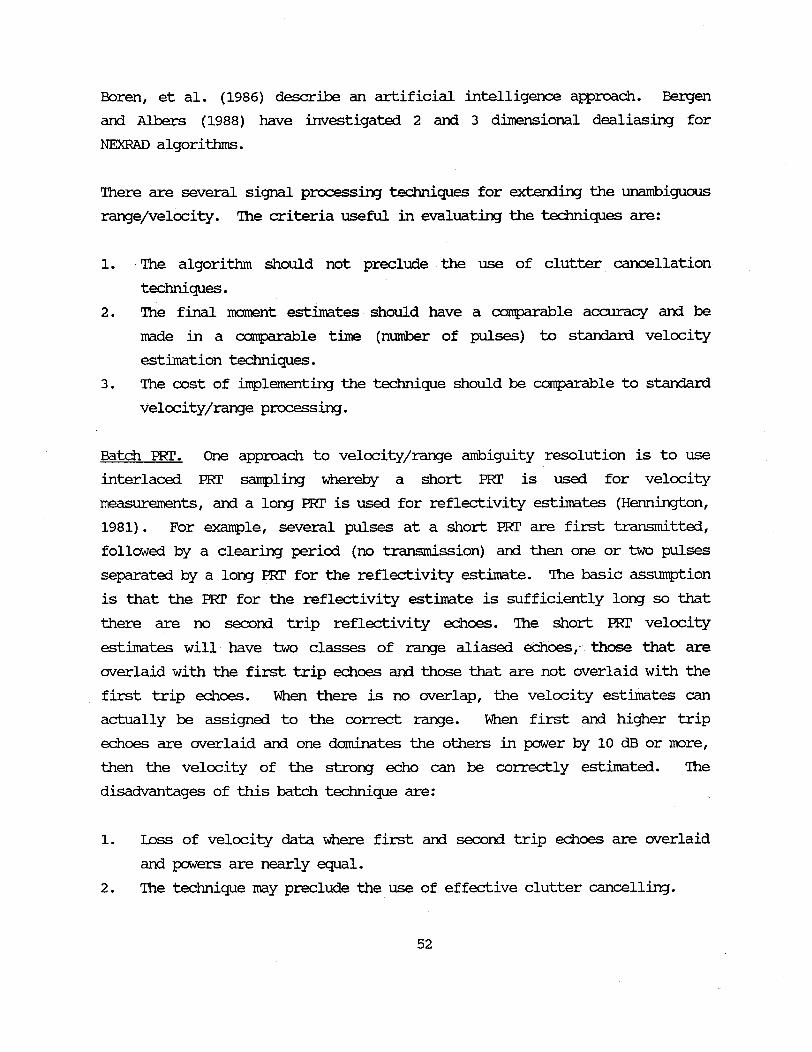
Boren, et al. (1986) describe an artificial intelligence approach. Bergen
and Albers (1988) have investigated 2 and 3 dimensional dealiasing for
NEXRAD algorithms.
There are several signal processing techniques for extending the unambiguous
range/velocity. The criteria useful in evaluating the techniques are:
1. The algorithm should not preclude the use of clutter cancellation
techniques.
2. The final moment estimates should have a conparable accuracy and be
made in a comparable time (number of pulses) to standard velocity
estimation techniques.
3. The cost of implementing the technique should be comparable to standard
velocity/range processing.
Batch PRT. One approach to velocity/range ambiguity resolution is to use
interlaced PRT sampling whereby a short PRT is used for velocity
measurements, and a long PRT is used for reflectivity estimates (Hennington,
1981). For example, several pulses at a short PTR are first transmitted,
followed by a clearing period (no transmission) and then one or two pulses
separated by a long PRr for the reflectivity estimate. The basic assumption
is that the PRT for the reflectivity estimate is sufficiently long so that
there are no second trip reflectivity echoes. The short PRr velocity
estimates will have two classes of range aliased echoes,- those that are
overlaid with the first trip echoes and those that are not overlaid with the
first trip echoes. When there is no overlap, the velocity estimates can
actually be assigned to the correct range. When first and higher trip
echoes are overlaid and one dominates the others in power by 10 dB or more,
then the velocity of the strong echo can be correctly estimated. The
disadvantages of this batch technique are:
1. Loss of velocity data where first and second trip echoes are overlaid
and powers are nearly equal.
2. The technique may preclude the use of effective clutter cancelling.
52

3. The data acquisition time is increased because the long PRT pulses are
unusable for making velocity estimates.
A similar approach is to have two radars share a common antenna which is
also known as a dual-frequency approach (Glover, et al., 1981). One radar
can sample at a long, constant PRT and the other can sample at a short,
constant PRT. Alternatively, two scans can be made at each elevation, a
long PRT scan for reflectivity and a short PRI scan for velocity. These
techniques are clearly more expensive but they allow excellent clutter
cancellation.
Multiple PRT and multiple PRF techniques can be used to dealias velocities.
Here, "multiple PRT" shall mean that the PRT is changed on a pulse-to-pulse
basis whereas "multiple PRF" shall mean that the PRF is fixed while a batch
of samples is collected and then changed for the next batch of samples. The
general technique is described by Sirmans, et al. (1976). Dazhang, et al.
(1984) and Zrnic and Mahapatra (1985) describe an actual implementation.
Dual PRT technique. In the dual PRT (or staggered PRT) method the two PRT's
usually are in ratios of either 3/2 or 4/3. First, one calculates the
first lag complex autocorrelation for each PRT, averaging over a number of
pulses. Then, the expanded velocity is calculated from
= (981 -2)/47r(T2-T 1) . (4.5)
The corresponding unambiguous velocity is
Vmax = + 4/4(T2-T1 ) . (4.6)
According to this expression, a 3/2 PRT ratio yields an unambiguous velocity
that is twice that corresponding to the short PRT, while for a PET ratio of
4/3, the expanded velocity range is 3 times. Why not expand further? Since
the variance of the expanded range velocity estimate is based on the
difference between the two fundamental estimates, its variance is roughly
proportional to twice that of each fundamental estimate. Fortunately, the
53

expanded velocity estimate need be used only to roughly dealias the two
fundamental estimates. The velocity estimate can be improved by averaging
the two velocity estimates to get the final estimator provided they have
been correctly dealiased. This averaging technique provides an estimator
that uses all available pairs of consecutive pulses, rather than half the
available pairs.
Since the dual PRT technique dealiases velocities by a large factor, one can
operate the radar at a lower PRF and thus have a larger unambiguous range.
Doviak and Zrnic (1984) point out that another advantage of the multiple PRT
technique is that second trip echoes will be incoherent or "whitened" and
thus not bias the first trip velocity estimates.
Dual PRF technique. A disadvantage of the dual PRT technique is that
standard clutter filters are very difficult to implement. This can be
overcome for some filtering schemes by using a dual PRF technique wherein a
sequence of pulses is collected at each of two PRF's and then each sequence
is processed separately. The data processing is identical to the standard
pulse pair processing except that the velocity from the previous sequence is
used along with the velocity from the current sequence to dealias the
current velocity. The sampling statistics are similar to the pulse pair,
except that for this technique to be viable the mean velocity change between
adjacent sequences must be small.
Because the PRF is fixed while each batch is collected, the dual PRF
technique can employ a batch processing clutter filter such as an FFT or an
FIR filter. An IIR filter can be used, but several pulses will be required
to clear the filter between PRF changes. Because the basic dual PRF
processing is essentially the same as standard pulse pair processing at a
constant PRF, it is easier to implement on an existing system.
Unfortunately, the dual PRT feature of "whitening" the second trip echoes is
lost when dual PRF sampling is used.
54

4.2.2 Resoluticn of range ambiguities
Low PRF radars minimize overlaid echo but require sophisticated velocity
dealiasing techniques. If we promote the occurrence of overlaid echoes by
using a higher PRF to provide a large unambiguous velocity, then the range
aliased echoes must be resolved.
Most range dealiasing techniques use phase codes to distinguish between
first and second trip echoes. The simplest is the "magnetron" technique for
which each transmitted pulse has a random phase. A typical magnetron is
coherent-on-receive only for the current pulse. This means that
contributions from multiple trip echoes are not coherent so that they appear
as increased white noise power. Consequently, the mean velocity and
spectrum width are unbiased by overlaid multiple trip echoes. A problem
with this technique is that the reflectivity cannot be deduced unless
various received noise sources can be evaluated quantitatively. Also, the
additional white noise that is caused by multiple-trip echoes reduces the
sensitivity to first trip echoes and degrades the accuracy of mean velocity
and width estimates.
A similar technique can be developed using a fully coherent system such as a
klystron in conjunction with a phase shifter to change the phase of the
transmitted pulse. This permits the transmission of pseudo-random phase
sequences that have "white" properties (Chakrabarti and Tomlinson, 1976;
Sawate and Dursley, 1980). The I and Q values can be "recohered" relative
to the first trip or the second trip, etc., by using the appropriate phase
shifts so that Doppler spectra can be evaluated for each trip (Laird, 1981).
This technique offers information for both the first and second trip
returns, but does not solve the problem of reduced sensitivity for overlaid
echoes.
Siggia (1983) addresses this issue by filtering the first trip echo from the
second trip echo and vice versa, to reduce noise contamination. The
technique works well as long as the two Doppler spectra (1t and 2nd trip)
are not so broad that they occupy a large fraction of the Nyquist interval.
Zrnic and Mahapatra (1985) have evaluated this technique.
55

Sachidananda and Zrnic (1986) describe a different technique where, instead
of inserting phase shifts to "whiten" the 2nd trip echo, the phase shifts
are inserted to cause the second trip Doppler spectrum to be a split bimodal
spectrum whose autocorrelation for lag 1 is zero. This means that the
second trip echo does not bias the first trip velocity estimates.
All of these "phase diversity" techniques are well suited for standard
clutter filtering techniques. However, there are substantial signal
processing computations to implement some of them.
4.3 POIARIZATION SWITCHING CO(SEQUENCES
Bringi and Henry (Chap. 19A) describe various polarization techniques which
provide valuable target information but make clutter suppression and
velocity dealiasing more difficult. Differential phase propagation,
scattering and instrumental effects preclude use of simple Doppler
processing techniques (Schnabl, et al., 1986). However, it is possible in
principle to extract both the Doppler information and differential phase
shift simultaneously (Sachidananda and Zrnic, 1989; Doviak and Zrnic, 1984).
Keeler and Carbone (1986) describe a dual PRT scheme which allows processing
two orthogonal polarization states separately prior to velocity dealiasing.
The alternating horizontal and vertical polarized pulse sequence mitigates
contamination caused by range aliasing since the overlaid second trip echo
is depolarized (Doviak and Sirmans, 1973).
Processing techniques to simultaneously provide clutter suppression,
velocity and range dealiasing, and polarization processing are just
beginning to receive serious attention.
56

5. EPDXRAfTORY SIGNAL PXCESSIN TECHXNIQUES
Implementations of modern signal processing algorithms on atmospheric radars
have evolved slowly in the last several years. Modern digital signal
processing algorithms have been difficult to implement for a variety of
reasons, but the algorithms are well known (Kailath, 1974). Programmable
processors with the speed to implement many of these algorithms and to
explore their application to distributed targets, rather than point targets,
is now possible.
5.1 PUISE OCfMPRESSICN
Pulse compression, or wideband waveform, schemes for improved radar range
resolution were first theoretically described by Woodward's (1953)
fundamental paper. Klauder, et al. (1960) and Cook (1960) later described
the linear FM (chirp) pulse which has been widely used in military radars.
Reid (1969) described a CW meteorological radar using pseudo-random coding.
Barton (1975) has edited a collection of pulse compression papers which
details the chirp technique. Lewis, et al. (1986) emphasize poly-phase
coded pulse compression waveforms.
Probably the first use of pulse compression for atmospheric distributed
targets was on the Arecibo ionospheric radar (Farley, 1969; Gray and Farley,
1973). The STORMY weather group at McGill University implemented a
compression scheme for reflectivity processing in the early 70's (Fetter,
1970; Austin, 1974). Their use was to provide many independent samples of
intensity within a given range cell to improve the reflectivity estimate.
They did not attempt any velocity measurements using their pseudo-random
phase coded pulse. In the late 70's Krehbiel and Brook (1979) reported
using a wideband noise waveform on the New Mexico Tech "Redball" radar to
provide reflectivity estimates during the short dwell time of their fast
scanning radar. Chadwick and Cooper (1972) and Keeler and Frush (1983a and
1983b) have described the principle of pulse compression Doppler
measurements on microwave weather radars using distributed targets.
Browning, et al. (1978) describe the 10 cm pulsed Doppler radar at Defford,
57

England which was modified to generate 4 Js, 5 MHz chirp pulses and measure
Doppler shifts from ice crystals at 8 km range. Chadwick and Strauch (1979)
demonstrated an FM-CW waveform on a 10 cm Doppler weather radar. Woodman
(1980b) shows how a continuous wave phase coded waveform was used in the
bistatic mode at Arecibo. Recently he has obtained full spectrum
information using this technique.
Pulse compression is a well established waveform design technique in the
military and aviation radar communities and has been used in the ST/MST
radar community (Crane, 1980; Gonzales and Woodman, 1984; Sulzer and
Woodman, 1985) and the lidar community (Oliver, 1979), but has not been
seriously investigated for microwave Doppler weather radar use. The reasons
for this are:
1. Range resolution and transmit power using standard high peak power
pulsed radars have been adequate to achieve the required scientific
goals.
2. Dwell times have been limited by mechanical scanning rates to tens of
milliseconds, thereby yielding the several independent samples of the
Rayleigh fluctuations necessary to obtain accurate reflectivity
estimates.
3. Presence of range time sidelobes on pulse compression waveforms causes
range smoothing and large bias errors in high reflectivity gradients.
5.1.1 Advantages of pulse omupression
The driving force for exploring pulse compression in weather radars is the
desire for ground based and airborne Doppler radars to rapidly sample the
volume at a spatial resolution adequate for mesoscale or cloud physics
analyses. These systems fall into the short dwell time category. Dwell
times of only a few milliseconds are insufficient for averaging independent
Rayleigh fluctuations to reduce the variance of parameter estimates.
Therefore, independence must be gained in some other way, in particular by
multiple frequency schemes or spatial averaging. Marshall and Hitschfeld
(1953) pointed out that frequency separations greater than the inverse pulse
width give independent Rayleigh returns. Pulse compression waveforms give
58

independent returns (to first order) at spatial resolution proportional to
the inverse bandwidth (Nathanson, 1969). Either technique gives independent
returns over short dwell times ( <5 ms) so that the antenna beam can be
scanned at least an order of magnitude faster than typical weather radars
(Keeler and Frush, 1983b). Strauch (1988) proposes a burst chirp waveform
relevant to short dwell time weather radars.
Another application of pulse compression waveforms is in solid state
transmitter systems which typically are peak power limited to low values
compared to klystron transmitters, but can sustain very long pulse widths
and generate average powers comparable to the tube systems with greater
reliability. Pulse compression techniques could be used with these high
duty cycle systems to achieve range resolution corresponding to a much
shorter pulse length. The NOAA network wind profilers will incorporate
pulse compression for this purpose.
5.1.2 Disadvantages of pulse ccmpression
There are tradeoffs associated with using pulse compression to achieve
faster scan time. The tradeoff involves reduced radar sensitivity with a
compressed pulse compared to a single frequency pulse of the same duration
and power. While the full benefit of the average transmitted power is
achieved, however the noise bandwidth must be increased to accommodate the
pulse bandwidth. Therefore, the SNR of the individual samples is degraded.
Keeler and Frush (1983a) describe how this tradeoff relates to the "time-
bandwidth product" (TB) of the compressed pulse. For the same average
transmitted power the increase in independence is TB and the decrease in SNR
is TB. For example, a chirp waveform 1 microsecond long sweeping 10 MHz of
bandwidth has a TB = 10. Range samples spaced by more than 15 m are
independent and have a SNR ten times lower than the uncompressed 1
microsecond pulsed waveform. Frequently, the independent range samples can
be averaged to provide estimates having a reduced variance while allowing
much faster scan rates.
The primary disadvantage is a contribution to the backscatter from range
time sidelobes. Because the receiver filter output is the cross-correlation
59

of the received waveform and the time reversed transmit waveform (a matched
filter), range time sidelobes will cause data "blurring" in range space
similar to that caused by antenna sidelobes in the transverse spatial
dimension. Range time sidelobes (and antenna sidelobes) are especially
troublesome in high reflectivity gradients. Because atmospheric targets are
distributed in space, it is the integrated sidelobes that contribute to the
distortion. They are analogous to the integrated antenna sidelobes which
contribute interference from distributed targets at the same range. The
contamination problem is particularly troublesome in downward looking radars
from air or space platforms when one desires to estimate precipitation
directly above the strongly reflecting earth surface. Careful waveform
design and tapering based on digital waveform generation rather than analog
devices may alleviate the range time sidelobe distortion (Farina, 1987).
For echoes with sufficiently long correlation times, as is the case of
ST/MST radars using long wavelengths, complementary codes (Golay, 1961;
Schmidt, et al., 1979; Woodman, 1980a; Gossard and Strauch, 1983; Wakasugi
and Fukao, 1985) completely cancel the range time sidelobes. However, more
robust schemes, like quasi-complementary codes (Sulzer and Woodman, 1984)
show good results in practice when non-linearities in the system distort the
desired pulse shape. The direct application of complementary codes is not
compatible with the shorter wavelength weather radar and lidar system.
The second disadvantage for pulse compression waveforms is the increase in
minimum range caused by transmitting a long pulse. Reception cannot begin
until the entire transmit waveform is finished. Pulses longer than several
microseconds are unacceptable for close ranges. The NWS wind profiler
solution is to extend the scan time using a short pulse mode for short
ranges and use a long pulse mode for long ranges. Other techniques also
exist.
A third disadvantage relates to the availability of bandwidth. Research
systems are not seriously constrained, but operational systems may require
bandwidths which do not fit into the channelized frequency assignments.
60

5.1.3 Ambiguity function
The tradeoff in sensitivity for a larger number of independent samples gives
considerable flexibility in waveform design - so much flexibility in fact
that the concept of the "ambiguity function" was developed by Woodward
(1953) to study the effects on range and velocity ambiguities for a specific
waveform. For our purposes this ambiguity function is indispensable for
understanding the receiver response to targets at other ranges and other
velocities from that to which the receiving filter is matched. Weather
targets are distributed in range and velocity by their very nature and are
especially sensitive to these undesirable responses.
The ambiguity function defines the ability of a waveform to resolve
different targets in range and velocity based on the power response of a
filter matched to some specific range time and Doppler shift (Nathanson,
1969; Skolnik, 1980; Brookner, 1977). Figure 5.1 shows the ambiguity
diagram for a single FM chirp waveform in range (r) and velocity (¢) space.
Note that targets having non-zero velocities at ranges different from the
desired range (r=0) contribute significantly to the filter output. The
function evaluated along the r axis (i.e., 0=0) is identically the
autocorrelation function of the waveform (Frank, 1963; Cook and Bernfeld,
1967; Barton, 1975).
Atmospheric radars involve estimation of the return power and velocity
rather than detection of such a target at some position in range-velocity
space. Our primary interest in the ambiguity diagram is to study the range
time sidelobes as a function of Doppler offset. It is easy to show that the
plot of the ambiguity function along the range axis is simply the
autocorrelation function. Real weather targets having Doppler shifts of
order only 103 Hz compared to pulse bandwidths of 107 Hz allow us to
concentrate our attention to this narrow strip of the ambiguity function
along the range axis. All the range time sidelobes in this strip must be
kept small to avoid contamination of targets at the desired range and
velocity. Known waveform design techniques may allow tailoring of the
waveform to our "small velocity" case to keep sidelobes in this narrow
61

Ijx (r, ) I
Io1O6 /
Fig 5.1 Ambiguity diagram for single FM chirped pulse waveform with TB=10.
r is range dimension. 0 is velocity dimension. Targets
distributed in (r,¢) space contribute to the filter output
proportional to the ambiguity function. For atmospheric targets,
Doppler shift frequencies are typically very small relative to
pulse bandwidth (Rihaczek, 1969).
62
I

ambiguity region acceptably small (Deley, 1970; Kretschmer and Lewis, 1983;
Costas, 1984; and Lewis, et al., 1986).
5.1.4 CCpariso with multiple frequency sdceme.
Krehbiel and Brook (1968) and Keeler and Frush (1983a) show that a pulse
compression waveform with time-bandwidth product TB has characteristics
similar to a multiple frequency radar using the same time and bandwidth
factors. Consecutive pulses may be generated at different frequencies and
processed in separate receivers tuned to the different frequencies. This
scheme yields the same number of independent samples for the same total
pulse duration and total bandwidth. The advantage of the multi-frequency
scheme, aside from the straightforward parallel receiver implementation, is
reduced range time sidelobes.
5.2 AiAPTIVE FJIIERING AIXIcTHMS
At Stanford University in the early 1960's, Widrow and his colleagues
(Widrow and Hoff, 1960) developed a class of filters that could "learn"
their received signal environment and, in time, adapt their characteristics
to optimally filter an incoming signal. Initial applications were in
pattern classification (Widrow, 1970), but use in adaptive antennas (Widrow,
et al., 1967) and the closely related field of spectrum line enhancement
(Zeidler, et al., 1978) and noise (interference) cancelling (Widrow, et al.,
1975a) quickly followed. Griffiths (1975) has described instantaneous
frequency estimation techniques applicable to Doppler radars. Atmospheric
radar applications (i.e., non-military) have been sparse mainly because the
computational load associated with constantly changing filter coefficients
could not be accommodated until recently. Keeler and Griffiths (1977) have
reported adaptive frequency estimation schemes applied to acoustic radars
sensing boundary layer winds.
With the advent of fast programmable signal processors, we can expect to see
a rash of new applications in radar for adaptive filtering techniques.
Adaptive filter systems are characterized by both a time variable transfer
function and the ability to self adjust, or be trained, to their environment
for optimizing some measurement criterion (Alexander, 1986b). A common
63

index for optimization is the minimum mean squared error (mmse) between the
processed output signal and a known desired output (or at least one which is
correlated with the desired signal). Figure 5.2 depicts a 2 dimensional (2
weight) error surface. Widrow's (1970) popular Ieast Mean Square (IMS)
algorithm estimates the gradient of the quadratic error surface and steps
the weights toward the minimum error value.
Nearly identical adaptive techniques have been developed for antenna beam
steering by Howells (1976), Gabriel (1976, 1980), Appelbaum (1976), Monzingo
and Miller (1980), and Compton (1988). Adaptive antenna systems have the
capabilities of tracking desired signals in space, maximizing the SNR, and
nulling out undesired interfering signals. The optimization criterion is
maximization of signal to interference plus noise ratio, which for many
cases is identical to the IMS criterion. For radar applications the beam
can be steered to the desired direction and the adaptation can
simultaneously maximize the SNR by spectral shaping and spatially nulling
any interfering sources. Van Veen and Buckley (1988) give a tutorial review
of spatial beam forming techniques.
5.2.1 Adaptive filtering applications
The structure for a performance feed back adaptive system is shown in Figure
5.3 where we note the input signal xk, the adaptive processor output yk, the
yet to be defined desired response dk, and the error signal, ek = dk - Yk.This error signal drives an adaptive algorithm which controls the transfer
function of the adaptive processor, and its output yk. Various closed loop
structures are possible as are a variety of adaptive algorithms. Widrow and
Stearns (1985), Honig and Messerschmitt (1984), Alexander (1986b), and
Haykin (1986) give excellent overviews of these structures and algorithms.
Widrow, et al. (1976) describe the learning characteristics of IMS adaptive
filters in both stationary environments when the filters converge to an
optimal setting and non-stationary environments where the filter continues
to adapt to the time variable input signal statistics. Adaptive filters
have found application in data prediction schemes, system identification or
modeling, parameter tracking, deconvolution and equalization, and
interference (clutter) cancelling (Alexander, 1986a). Usually the
64
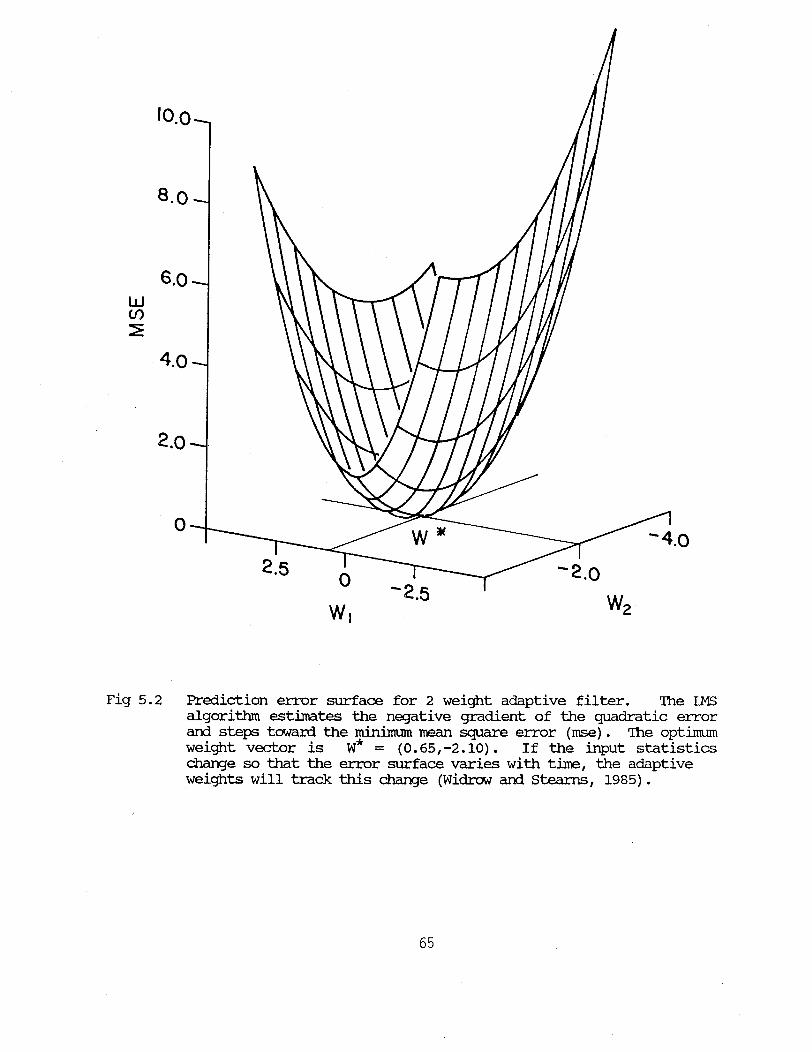
LU()2
.0
WIWI W2
Fig 5.2 Prediction error surface for 2 weight adaptive filter. The LMSalgorithm estimates the negative gradient of the quadratic errorand steps toward the minimum mean square error (mse). The optimumweight vector is W* = (0.65,-2.10). If the input statisticschange so that the error surface varies with time, the adaptiveweights will track this change (Widrow and Stearns, 1985).
65

Inni it
Xk
Errork
Fig 5.3 Adaptive filter structure. The desired response (dk) isdetermined by the application. The adaptive filter coefficients(Wk) and/or the output signal (Yk) are the parameters used forspectrum moment estimation (Widrow and Stearns, 1985).
66
application determines the origin of the reference signal and the specific
adaptive algorithm to be used. Sibul (1987) has edited a collection of
application papers for adaptive filters. Further applications in neural
networks and fault tolerant computing are being explored (Lippmann, 1987;
Shriver, 1988).
As an example of an atmospheric radar application, an adaptive linear
prediction filter will improve the SNR of the received signal so that the
moment estimation will yield improved estimates. In the frequency domain
the prediction filter acts as a narrow band pass filter having time variable
center frequency which passes the received signal while suppressing the
spectral noise components. Tufts (1977) and Anderson, et al. (1983)
describe this enhancement procedure. The input signal xk is the desired
signal, dk. The previous input samples (xkl, xk_2, ..., xk-L} = XT are
filtered to predict, or estimate, the present sample xk. The error signal
is the difference between Xk=dk and its estimate Yk, i.e. ekx-yk. The
filter is adjusted using the IMS algorithm so that the mean squared error
signal <ek2> is minimized. Sequentially then, the filter adjusts itself to
predict the input signal more accurately. Some error will be present but
the predicted signal will have an improved SNR over the input itself. In
this sense, we have an adaptive matched filter which can track the input
signal as its characteristics (e.g., its Doppler shift and width) change
with time (Tufts and Rao, 1977).
Probing deeper into the mathematics, we find that the algorithm is
estimating the negative gradient of a quadratic error surface in the L
dimensional adaptive filter weight vector space and adjusting the filter
weight vector Wk to step towards the minimum mean squared prediction error
with every iteration. This operation plus some supporting mathematics
defines the highly efficient steepest gradient descent IMS adaptive
algorithm (Widrow, 1970; Widrow, et al., 1975b).
Wk+l = Wk + 2gek Xk, (5.1)
67

where g is a precisely defined constant which determines the convergence
rate and the excess noise generated by the adaptation process.
It is easy to show that the one step prediction structure leads to the Lth
order maximum entropy (ME) spectrum estimate (Lang and McClellan, 1980;
Griffiths, 1975). Keeler and Lee (1978) have shown how the complex, first
order, one step prediction filter yields the pulse pair frequency estimator,
which has been made adaptive. Keeler (1978) further reports a bias and
variance of an adaptive ME frequency estimator.
What makes adaptive prediction and SNR enhancement possible is the
difference in correlation time of the desired narrow band signal (or
sinusoid) and the unpredictable white noise. Similarly, the long coherence
time of clutter input components may allow these interfering signals to be
rejected using adaptive interference (noise) cancelling filters (Widrow, et
al., 1975a). For example, airborne Doppler clutter can be represented by a
strong, narrow spectral return having a variable Doppler shift and sea
clutter may be sufficiently offset from zero Doppler that an adaptive scheme
may provide adequate suppression in both cases.
5.2.2 Adaptive antenna applications
Adaptive beamforming was motivated by a desire to steer the main beam in a
desired direction while simultaneously nulling interfering sources and
maximizing the signal to interference plus noise ratio at the output of the
adaptive beamformer (Haykin, 1985a; Compton, 1988). Atmospheric radars are
troubled by interfering ground clutter returns and could benefit from using
an adaptive antenna. For example, an RHI scanning radar could dynamically
place a line of nulls along the dominant ground clutter return angles near
0° elevation. Or a ground reflected multipath ray could be suppressed. UHF
radio communications present slowly time varying interfering sources for
wind profilers which could be suppressed by adaptive array techniques.
Forming nulls in the array antenna patterns in real time as the interferers
become active or as the antenna elevation increases may be feasible in many
cases. Constraints on the adaptation speed and antenna scan rates may limit
68

performance of these proposed systems since stationarity over a finite time
period is usually required. Furthermore, narrowbeam systems require several
thousand array elements and a digital control system for a truly adaptive 3
dimensional beam. Cost is a limiting factor in this regard (Mailloux,
1982).
Array processing utilizes multi-channel processing algorithms to process the
individual signals from each element to effect both spatial beamforming and
temporal filtering. Vector and matrix based algorithms introduce special
difficulties. Haykin (1985a) describes array signal processing algorithms
which have been applied to a variety of fields, e.g. seismology, radio
astronomy, tomographic imaging, sonar, and radar. Recently, Sachidananda,
et al. (1985) have proposed sequentially changing (at the pulse repetition
rate) the pattern of a phased array antenna. Subsequent Doppler processing
allows contributions to velocity estimates entering through the antenna
sidelobes to be whitened and/or removed (Zrnic and Sachidananda, 1988).
5.3 UITI-CHANNEL PRDCESSING
As atmospheric remote sensors become more sophisticated and programmable
processors achieve greater computational power, multi-channel processing
algorithms will become more common. The signals from separate input
channels can be thought of as a vector time series and processed, or
filtered, collectively by using the correlated information in the channels
to produce more accurate parameter estimates than if they were processed
separately (Marple, 1987). The coefficients of these multi-channel filters
are found by solving a set of linear equations similar to the single channel
equations used in linear prediction filtering and associated applications.
Wiggins and Robinson (1965) give a recursive technique for solving these
"normal" equations. Strand (1977) and Morf, et al. (1978) describe multi-
channel maximum entropy spectrum estimation, which is a direct result of
solving the normal equations.
In addition to radar array antenna data, dual polarization data is another
example of a multi-channel complex input signal. Horizontal and vertical
channels of a dual linear polarization radar can be processed to yield cross
69

parameters. Each input data point can be thought of as a 2x2 matrix, the
polarization matrix, rather than a complex I and Q estimate. The set, or
vector of these matrix inputs is then processed using complex matrix
algorithms which are designed to optimally and jointly estimate target
parameters. Processing both channels simultaneously yields additional
information that could not be obtained if they were processed independently.
Integrated sensor systems can benefit by multi-channel processing schemes.
A multi-channel algorithm might make use of 10 minute wind profiler data and
1 minute radar or lidar data. Wind profiles on multiple scales would be
produced with lower error than either system operating alone. Application
of coherence functions to these multi-channel sensors provides an analytic
tool for correlated data which improves the analysis.
5.4 A IPRICI INFR4ATICN
Information that is known in advance, a priori information, can be used to
improve atmospheric parameter estimates. Most remote sensors treat each
spatial resolution volume independently from all others. However, there are
physical constraints in the atmosphere that limit the rates of change of
certain parameters. These constraints are known in advance and can be used
to constrain the processing algorithm to produce better estimates of
velocity, for example, than if they were ignored. To be most effective this
a priori knowledge should be used as early in the processing chain as
practicable. For example, if one knows (or is confident that the received
signal consists of a Gaussian shaped signal spectrum in white noise, then
one should be able to use this prior information to generate a lower error
velocity estimate than if the information were ignored.
Signal processing algorithms constrained by known a priori information
typically yield simpler and faster algorithms that give lower variance
estimates than unconstrained estimators. Frequently these estimators are
maximum likelihood, i.e., minimum variance, and can be readily computed
using modern processing hardware.
70

6. SIGNAL PFXFESSCR IMPTrFMTATION
Signal processing encompasses analog and digital processing of both the
transmitted and received radar signal. Because of timing requirements, most
pulse-to-pulse control functions are also handled by the signal processing
system. In this section we discuss the signal processing implementations
that are found on modern radars and the tasks typically allocated to the
signal processor.
6.1 SIGNAL PROCESSING CONTROL FUNCTICNS
Signal processors usually perform a variety of radar control functions and
serve as the interface between the radar system and the radar data
processing system (usually a host computer). These control tasks include:
1. Pulse waveform selection
2. Polarization switching
3. Phase sequencing
4. Pulse sequence generation
5. Range gate trigger generation
6. Linear channel gain control
7. Calibration pulse injection
Radar control starts at the transmitter. The signal processor usually
generates the PRF, although good practice dictates that the basic clock be
derived from a reference oscillator that is shared between the processor and
the radar. PRF control by the processor minimizes the possibility of range
bin jitter caused by timing uncertainties in the A/D sampling and is
particularly important if a multiple PRF processing scheme is employed since
the processing must be synchronized with the PRF.
Because of the need to preserve the duty cycle limit of the transmitter, it
is a safety feature and a convenience to have the signal processor also
control the pulse width and bandwidth filter selection.
71

Since the signal processor is in control of the PRF, it is typically
assigned the task of controlling all pulse-to-pulse functions such as phase
control for pseudo-random phase processing and polarization switch control.
This approach assures that the processing is properly synchronized with all
aspects of the transmit-receive sequence.
Built-in calibration test units that operate during normal data collection
are now found on some systems. The idea is to inject a pulse of known power
and phase characteristics in the last few range bins for each transmitted
pulse or during antenna repositioning intervals with the transmitter off.
These bins are then processed identically to all other bins. The output
values can be monitored in real time to verify that the system is
functioning properly, and for system power calibration. In addition, the
injected signal can be made coherent so that the Doppler processing can be
checked. The advantage of this approach is that the entire receiver and
processing system can be verified without interrupting normal operations.
The remainder of this section is devoted to linear channel gain control
techniques. Currently, the receiver systems for most applications use
analog signal -processing techniques for deriving the linear channel I and Q
(in-phase and quadrature) and log channel outputs. The log channel output
is typically used for quantitative power measurements because of its dynamic
range capabilities (90-100 dB). The linear channel measurements are used
for extracting information related to the phase of the signal, i.e., mean,
velocity, spectral width and clutter measurements, and can provide power
estimates as well. The linear channel measurements operate over a more
restricted dynamic range, typically z40-60 dB, that is usually shifted by
means of an automatic gain control (AGC) loop over a range of ~100 dB. It
is the linear channel gain control problem where digital signal processing
often makes its first appearance in the radar processing chain.
Linear receiver gain control is typically performed via one of the following
methods:
1. IF limiting
72

2. Sensitivity time control (STC)
3. Slow AGC
4. Fast AGC
5. Multiple receivers
In the first case, a "soft" limiter is inserted at IF before phase detection
(Nathanson, 1969; Zeoli, 1971; Frush, 1981 ). The advantage of this
technique is that it is extremely simple to implement and permits the linear
receiver to operate over a fairly wide dynamic range with good mean velocity
retrieval. However, if the Doppler spectrum is bimodal, such as for ground
clutter mixed with a weather spectrum, this technique tends to "capture" the
stronger signal and suppress the weaker one. This behavior makes it
unsuitable for systems that require clutter cancellation.
For the STC case, the linear channel gain is increased with range in an
attenpt to represent the average characteristics of weather and clutter.
Since there is no feedback based on actual power measurements, it is easy to
implement. However, it is a near certainty that strong clutter targets will
cause saturation of the linear receiver at close range unless an IF limiting
approach is used as well. Likewise, weak clear air echoes that would be
detectable at full gain at close range, will be attenuated beyond
detectability.
For the slow AGC, the log receiver measurements from the previous ray are
used to optimize the linear receiver gain for the targets that are actually
present at each range. The samples for an integration period are collected
while the gain is held constant. If the log receiver is used for
quantitative power measurements, the actual gain does not need to be known
with great precision (within 3 dB is usually satisfactory). Also, since the
gain is held constant, the phase shifts that are introduced by the gain
control are constant from pulse-to-pulse so that these do not have to be
corrected. The primary drawback is that the ability to distinguish between
the clutter and weather components of the signal may be limited by the
fundamental dynamic range of the linear receiver. Furthermore, strong
reflectivity gradients will cause erroneous gain settings.
73

The fast AGC, or instantaneous AGC (IAGC) approach, for which the gain of
the linear receiver is adjusted for each range and each pulse, is used where
there is a high degree of phase purity in the transmitted pulse (e.g.,
klystron systems). The power measurement for either the previous pulse, orthe current pulse (in which case a delay line is required) is used to set
the receiver gain. This is the most complicated form of AGC to implement
since it requires a very accurate calibration of both the amplitude and
phase response of the receiver as a function of gain and the input power.
Mueller and Silha (1978) employ a real-time calibration and correction
scheme so that the output phase of the linear receiver requires no
correction. Properly implemented this approach provides wide dynamic range
linear response for high-performance clutter cancellation and more accurate
estimates of the power than a log channel.
Another approach is to employ multiple receivers, each optimized for a fixed
range of input power with the advantage that all samples can be digitized
and the optimal receiver can be decided with a digital algorithm. Moreover,
switching transients and calibration procedures are minimized.
6.2 SIGNAL A/D CONVERSIC N AND CAIBRATICN
Figure 6.1 shows a block diagram of a typical digital, time domain Doppler
signal processor. The digital signal processor provides the interface to
the radar I, Q and log signals, and connects to a host computer that
provides the user interface, data processing, display and data
communications.
After analog phase detection, the I, Q and log values are digitized. In the
case of a fast AGC, a digital AGC value may also serve as an "exponent" for
a floating point representation. The precision that is required for
digitizing the I and Q values depends primarily on the underlying precision
of the linear receiver and the dynamic range limitations imposed by ground
clutter induced phase noise. In computing dynamic range, an additional bit
amounts to 6 dB more power measurement capability. However, because the
receiver noise level requires about two bits to coherently integrate weak
74

g
ication
Fig 6.1 Block diagram of a typical signal processor.
75
signals and one bit denotes the sign of bipolar data, the usable
instantaneous dynamic range is limited to ~54 dB for 12 bit samples. This
range provides a margin for an AGC that may not optimize its use of the
receiver dynamic range and offers reasonable clutter rejection. For the log
channel, the quantization of the digitized signal determines, to some
extent, the accuracy of the final power estimates. However, it is usually
the inherent large fluctuation of «30 dB for Rayleigh signals (Nathanson,
1969) that imposes the more fundamental limit.
The A/D converter values should not saturate. I and Q saturation causes
harmonic generation in the frequency domain. Furthermore, image spectrum
generation about DC in the spectrum is frequently caused by imbalance in the
amplitude and/or phase of the I and Q signals (Hansen, 1985).
Time domain averaging is an important step in processing ST/MST radar
signals to reduce the noise (Strauch, et al., 1984). The averaging not only
increases the SNR by N, but also increases the dynamic range by 10 log N.
The discussions above illustrate the need for time series and power spectrum
displays to optimize radar performance. Just as important, the host
processor must be equipped with software to provide the interactive displays
that are required for accurate system adjustment and verification.
6.3 REEIETlVlTY PROCESSING
The precise measurement of the received power is an important objective for
most weather radar systems, and for noncoherent systems, this is the primary
measurement. In the pre-Doppler era, there was interest in the so-called
"power-fluctuation spectrum" and spectrum width estimates (Rutkowski and
Fleisher, 1955; Atlas, 1964;). Most radar systems, whether Doppler or
noncoherent, employ a wide dynamic range log receiver that operates at IF.
These systems merely average the log values which results in an asymptotic
(with the number of independent samples) 2.51 dB bias in the estimation of
the average power for Rayleigh distributed targets (Doviak and Zrnic, 1984).
There are other types of receiver responses, such as the linear and square
law receivers, and the log receiver has the largest standard deviation for
power estimates (Zrnic, 1975a). However, in view of calibration errors and
76

the uncertainties in relating power measurements to rainfall rate, the log
receiver performance is adequate for many applications. When differential
reflectivity measurements are required, one attempts to measure small
differences in power so that the square law receiver is preferred (Bringi,
et al., 1983; Chandrasekar, et al., 1988).
Two common techniques that are used for power averaging are the exponential
average (Zrnic, 1977a) and the uniformly weighted average. Exponential
averaging is calculated using
Pk = Pk-1 *(1-C) + Pk *C (6.1)
where Pk is the current estimate of average power based on the new sample pk
and the previous estimate Pk-1 . C is a weighting constant between 0 and 1.
When C is close to 1, the current pulse is more strongly weighted. This
technique is extremely simple to implement in real time and provides a new
estimate for each pulse. Since real time digital processing capabilities
have improved, and analog CRT displays are rapidly being replaced by color
displays, this technique has been largely replaced by a simple uniformly
weighted average over a fixed number of pulses.
Averaging of independent samples is required to obtain accurate reflectivity
estimates. Since. independence is governed by the coherence time this
imposes a fundamental constraint on the scan rate for data collection. For
example, at 3 rpm and 500 Hz PRF, one can average only 27 pulses per degree
of antenna rotation. Depending on the wavelength and the spectrum width of
the scatterers, not all of these pulses will be independent. A technique
for increasing the number of independent pulses is to average in range using
a range bin spacing that is greater than the pulse width. This requires
somewhat more processing power, but results in more accurate reflectivity
estimates. Also, averaging can be adjusted as a function of range so that
the resulting average range interval is comparable to the beamwidth
dimension.
77

The conversion from dBm to dBZ is done via the radar equation which involves
the radar constant and range normalization. The term "STC" is sometimes
inappropriately used to refer to the digital range normalization that isperformed in the processor. This term is a reference to the analog
technique that was used in the past to represent the radar reflectivity on
CRT display. Digital range normalization merely adjusts the output values
appropriately without causing the loss of sensitivity at short range.
6.4 'THRESHOEIDfING R DATA QUALITY
The goal of thresholding is to have the signal processor flag data that
may be corrupted by bias and artifact. Clarity of presentation of the
spectral moments is important to a user trying to interpret a display. Forsubsequent data processing and product generation (e.g., CAPPI's, cross-
sections, rainfall accumulations), noise, bias and other artifacts increase
the computational demand on the data processor and degrade the final
product. Finally, thresholding followed by run length encoding for data
compression can greatly reduce the communications bandwidth requirements for
transmitting radar data and products and reduce the archive resources that
are required to store them.
There are numerous thresholding criteria and variables that are employed in
modern radars:
1. Incoherent signal-to-noise power
2. Coherent signal-to-noise power
3. Doppler spectrum width
4. Clutter-to-signal power
5. Zero velocity
6. Geometric criteria
7. Statistical criteria
The incoherent signal-to-noise power is calculated by comparing the received
power at a range bin with the system noise power (S+N/N). This criterion is
most commonly used to threshold the wide dynamic range power measurements
(e.g., from a log receiver). The coherent signal-to-noise power is the area
78

under the signal portion of the power spectrum divided by the total noise
power (S/N). It can be calculated directly from the spectrum, or using the
measured autocorrelations. Similarly, the spectrum width itself can be used
as an indicator of the accuracy of the Doppler mean velocity and spectrum
width.
Both a low coherent signal-to-noise ratio and a large spectrum width
contribute to a large variance in the velocity and width estimators.
Ideally, thresholding should be made at a constant variance level, e.g.,
velocity is accepted if it's expected error is less than 1 m/s.
Unfortunately the relationship that governs the effect of SNR and width on
the variance of the velocity estimator is not a simple one (Zrnic, 1977b),
hence it is usually not implemented as a real time thresholding criterion.
Instead, the typical approach is to use either the coherent SNR and/or the
width separately and adjust the threshold until the displays are reasonably
free of speckles.
A popular measure of the quality of velocity and width estimates, which
accounts for the effects of both the coherent SNR and the spectral width is
the normalized first lagged autocorrelation magnitude IR(1)|/R(O). It is
easily computed, conveniently bounded between 0 and 1 and thresholds
unreliable estimates reasonably well.
The measured clutter-to-signal ratio (CSR) is often calculated for the
purpose of correcting the log receiver power for the effects of clutter.
When the actual CSR exceeds the dynamic range capabilities of the receiver
or the ability of the clutter filter to accurately remove clutter, then the
data should be discarded. The calculated CSR can then be used as the
thresholding criterion.
Another method of thresholding range bins that are affected by clutter is to
simply not display bins that have a mean velocity within a narrow band about
zero velocity. This technique is effective for Doppler radars that have no
clutter filter, or Doppler radars of limited linear dynamic range available
for cancelling clutter. Both the velocity and reflectivity can be
79

thresholded using this criterion. Unfortunately, any weather that falls
into the threshold velocity band is also rejected.
Simple geometric considerations can be used for thresholding data that are
not physically reasonable. A very simple threshold is to eliminate all data
that are above a fixed height where weather echoes are assured not to occur,
e.g., 20 km. Another threshold that is easily implemented in a processor is
a "speckle remover" that eliminates all isolated range bins that have no
nearest neighbors in range or azimuth. Use of a speckle remover eliminates
aircraft and point clutter targets. It also allows other thresholds to be
set to lower values for greater sensitivity since only double speckles will
be passed.
Finally, statistical criteria involve considerations of local continuity and
rejection of data that are a few standard deviations away from local mean
values. Strauch, et al. (1984) utilize a very effective "consensus
averaging" technique (Fischler and Bolles, 1981) to delete wild points or
outliers for time domain integration of wind profiler processing. One or
two dimensional median filtering techniques also allows deletion of
individual or isolated groups of anomalous data.
The application of thresholding requires caution. One common problem
develops when a linear channel index is used to threshold both the velocity
and the reflectivity. If this is done it is not uncommon to observe "black
holes" of rejected reflectivity echo (so called if the display background is
black). These often occur in regions of large shear or turbulence such asthunderstorm cores (Hjelmfelt, et al., 1981) where there is ample
reflectivity present. This points out that different threshold
combinations, and perhaps threshold levels, should be used for the different
spectral moments. For example, an acceptable threshold for velocity will
generally not be appropriate for spectrum width since spectrum width
requires a stronger signal for proper estimation.
80

7. ITREND IN SIGNAL PROCESSING
7.1 REALIZATIC[N FACT
Several key components comprise a realizable signal processing system--
chips, memory, and a large bandwidth output device. This digital technology
has found wide applications in modern radars (Rabinowitz, et al., 1985).
7.1.1 Digital signal processr chips
In the last 5 years integrated circuit chips specially optimized for digital
signal processor (DSP) operations such as multiply-accumulate, on-chip
memory, and the supporting logic have developed computational power
exceeding hardwired processors of several years ago. These DSP chips are
available from a variety of manufacturers and can be installed on
commercially available high speed busses, such as VME and Multibus II. As
integrated circuit developments in memory continue, on-chip memory will
expand to allow caching and make DSP algorithm's more efficient.
Interconnectability using multiple fast busses and fast communication ports
still allow full implementations of many DSP algorithms. The commercial
availability of families of DSP chips and busses provides documentation,
technical support, and probable upgrades for faster and compatible
processing speed.
Current 32 bit DSP chips are based on silicon technology (TTL and CMOS) and
can achieve clock rates of tens of MHz and execution rates of a few Million
Instructions Per Second (MIPS). The next generation of microprocessor and
DSP chips will be fabricated from gallium arsenide (GaAs) and will allow
several processors to be attached to a single chip component. Clock rates
for these advanced devices will be a few hundred MHz with instruction rates
exceeding 100 MIPS. This technology is growing rapidly. However, within
the next several years the number of components per chip will be limited by
fabrication processes and shortly thereafter by physical constraints within
the chip itself (Aliphas and Feldman, 1987).
81

An important factor that will allow rapid expansion of radar processing
power is the trend of D6P chip manufacturers to develop higher performance
chips that are compatible with previous versions. Thus, a relatively simple
redesign of the processor board using the same basic architecture, combined
with reprogrammed algorithms, offers greatly enhanced processing power at
low cost.
The ready availability of the processing power obviates a move towards more
real time processing. For example, as multi-parameter radars and faster
scanning radars evolve, more processing power will be necessary to compute
the quality-checked, auto-edited data that is so valuable to real time
observations. The real time processing can perform all the "signal
processing" plus an increasing amount of the "data processing" tasks.
7.1.2 Storage media
External devices for mass storage have long been dominated by magnetic tape.
The half inch tape is the standard, but various other tape-based media and
technologies are being explored. These include special high density tapes
such as NCAR's obsolete TBM (terra-bit memory), magnetic tape cartridges,
video cassettes, and the digital audio tape (DAT) devices using helical scan
technology. All of these tape storage media suffer from serial access
delays and are undesirable for on line, fast access storage. However, they
are extremely well suited for "write-once" archiving applications such as
radar data acquisition. Storage capacities of two or more gigabytes can be
achieved today. Higher capacity and faster transfer rates will continue to
evolve. Winchester disks using "vertical recording" techniques allow high
density and fast access and fit many applications which require fast, random
access storage.
The thrust in storage media development now seems to be in optical recording
techniques. Compact disk (CD) technology, being a consumer product, has
become relatively inexpensive. The data capacity of optical media is
approaching several Gbytes on a 5.25" CD and data transfer rates of several
Mbytes/sec are possible. Random access times are being reduced to the
millisecond range.
82
7.1.3 Display technology
Real time color radar displays have become an important component of remote
sensor technology since their first implementation by Gray, et al. (1975).
Intensity modulated PPI and RHI scopes show high resolution reflectivity
displays, but digital color displays show all the directly measured
variables (e.g., velocity) as well as derived variables such as differential
reflectivity, phase, and depolarization quantities. Plotting data from
multiple sensors in real time, zooming into specific areas of interest,
generating time lapsed images, and defining special overlays provides a
measure of flexibility not available only a few years ago. Special purpose
programmable graphics processors allow these new, yet fairly simple, image
processing capabilities. The next generation of graphics processors will
accommodate 3 dimensional real time image generation, color images with
transparency, easily manipulated images to change the viewing angle, and
programmability in high level languages to allow a high degree of user
interaction. The display is the investigator's or the user's contact to the
environment being studied or watched. Particular emphasis should be placed
on this aspect of the remote sensor to extract its maximum utility.
7.1.4 omrmercial radar processors
Radar processors have historically been developed by the organization
responsible for the entire remote sensor system. Recently, however, digital
signal processors have become commercially available as special purpose
computers for Doppler lidars (Bilbro, et al., 1984), and weather radars
(Siggia, 1981; Chandra, et al., 1986, and Schroth, et al., 1988). The
specialized processing algorithms being developed and applied to atmospheric
remote sensors can be efficiently integrated into many types of remote
sensors and customized to the specific application by different software.
System engineering of signal processors is changing because of the
improvements in hardware technology and architectures (Allen, 1985).
However, the biggest change is occurring because of changes in the system
engineering methodology. Open software standards for operating systems
83
(e.g., POSIX), for computer language (e.g., ANSII standards, Ada, etc.), and
run-time environments (e.g., X-OPEN) are being developed and applied. Data
bus standards, (e.g., VME) are being clarified, updated and adhered to by
board and peripheral manufacturers. Open software standards and workable
data bus standards facilitate cost-effective development and manufacture of
special signal processing boards that integrate and can be upgraded to the
latest DSP chip sets.
7.2 IREN1&S IN I EGRA4TBILr[TY OF DSP
The new generation of digital signal processors for atmospheric remote
sensors is programmable. This is a marked contrast to early hardwired
processors in which the algorithms could be modified only with great
difficulty and most often resulting in the loss of the original capability.
Programmable processors allow algorithm modifications, processing
experiments, diagnostic testing, and system testing while still retaining
the capability of returning to a pre-existing mode of operation. Modern
digital filtering and waveform processing using advanced algorithms is now
possible without the constraints imposed by physical limitations of hardware
devices. Schmidt, et al. (1979) and Woodman, et al. (1980) describe
programmable signal processors for VHF Doppler wind profilers. These
present day DSP systems are directly programmable in modern languages, such
as "C".
Advanced processing algorithms using matrix methods, such as singular value
decomposition, orthogonalization, multichannel optimization techniques, and
non-linear processing algorithms using adaptive and data compression
techniques (Haykin, 1985a; Kay, 1987; Marple, 1987) can be coded and tested
on line in real time, without destroying the original algorithm
implementation. Standard algorithms can be as easily replaced as they can
be modified. Optimization may become an easier task.
As the DSP chips support higher level languages, algorithm portability
becomes easier to achieve. Reproducability of clone processors and
algorithms, for example in a radar network, is feasible. However,
programmable hardware leads to a new set of development and maintenance
84

problems. A higher level of training and maintenance equipment is required
for trouble-shooting a malfunctioning radar processor. Board level
maintenance may require a more expensive spare inventory. Programmability
brings new headaches as well as many new features.
Another area of rapid development important to distributed signal processor
architectures is the application of multiprocessor operating systems.
Distributed computing power on a common high speed bus requires an operating
system capable of controlling data transfers and bus arbitration and memory
management. Presently these operating systems are targeted towards more
general purpose processor chips (e.g., the Motorola 68030), but future
application will find them on distributed DSP processors as well. Software
development is a key issue in generating efficient realizations of the DSP
algorithms. UNIX is presently becoming accepted as the common operating
system of choice for many applications programs and for development of real
time software, which then typically run under a UNIX compatible real time
operating system (e.g., VxWorks, PDOS).
7.3 SHIOR TERM EXPECCTATICNS
During the next 5 years we may expect a revolution in atmospheric digital
signal processor technology. However, this technology will tend to leave
the atmospheric science community behind unless we prepare ourselves to take
advantage of the evolving hardware and software advances. We have lived by
the pulse pair processor for over a decade. Other techniques have been
explored that in same instances provide better parameter estimates but have
not been feasible to implement in the past. This constraint is rapidly
disappearing.
7.3.1 Rarge/velocity ambiguities
Within the next 2 or 3 years we may expect several research groups to
implement new pulsing and processing schemes for range and velocity
dealiasing. These schemes, driven by the FAA's Terminal Doppler Weather
Radar (TDWR) procurement, as well as the Nexrad implementations, will allow
ground clutter suppression simultaneously with velocity dealiasing and
overlaid echo suppression algorithms. There will be exploration of
85

polarization processing improvements combined with resolving range and
velocity ambiguities and clutter suppression.
7.3.2 Ground clutter filtering
Effective clutter filtering will be readily implemented on conventional
Doppler radars. However, efforts to integrate clutter suppression with
other processing improvements will likely encounter several technical
obstacles involving analog components (e.g., polarization switches, IF
amplifiers, and transmitter instabilities). Fundamental limitations related
to the narrow clutter spectra may well limit clutter suppression for radars
using dwell times shorter than the clutter correlation time. Yet to be
explored nonlinear filtering techniques may allow effective suppression even
under these conditions.
7.3.3 Waveforms for fast scanning radars
A major limitation of existing Doppler meteorological radars is their
inability to scan a solid angle in space fast enough to measure a rapidly
evolving atmospheric event with adequate temporal resolution. A dwell time
of a few milliseconds is desired. The proper long term solution requires an
electronically scanned phased array antenna - a very expensive item. The
mechanical solution of simply scanning faster and using short dwell times is
insufficient to preserve the parameter measurement accuracy. Scan rates
greater than about 100 degrees per second for a 1° beamwidth cause spectrum
spreading due to antenna motion that rapidly degrades the measurement
accuracy. A reasonable alternative is to rapidly scan mechanically at a
rate such that the spectrum spread is not dominated by the scan induced
component and to use a wideband waveform (pulse compression or multiple
frequency) that allows a reasonably large number of independent parameter
estimates to be made in the short dwell time imposed by the coherence time
of the return signal. Some research groups are testing short dwell time
waveforms (Keeler and Frush, 1983b; Strauch, 1988) on both airborne and
ground-based weather radars.
86
7.3.4 Data cmpression
Data compression algorithms are an important aspect of signal processing.
Data compression can be divided into two classes -- "truncation" for any
range gates at altitudes greater than the tropopause and "run length
encoding" or "compaction" for strings of data having the same value.
Typically parameter estimates not passing some threshold test are
arbitrarily set to zero and run length encoded. Data truncation will become
more common as programmable processors are installed.
7.3.5 Artificial intelligence ased feature extraction
Future computing will be directed at enhancing man's analytical and
inferential skills, rather than routine physical or mental activities.
Symbolic programming techniques combined with knowledge engineering and
artificial intelligence techniques show potential for rapid advance; the
same is true for meteorological image processing and automated recognition
and extraction of atmospheric features. Two dimensional signal and image
processing algorithms will be implemented using programming architectures,
reducing development time and extracting more meteorological information
from remote sensor data sets.
7.3.6 Real time 3D weather image processing
Relatively new computing hardware allows ready implementations of various
symbolic object processing systems that can be applied to problems in
atmospheric science. Coupled with fast graphics processors we can expect
real time 3D images produced with the latest image rendering techniques
which allow reconstructed radar data fields overlaid with in-situ
measurements from airborne and ground based meteorological stations.
Graphics computers with large video memories allow time lapsing of high
resolution 3D images and arbitrary cross sections to be displayed using a
variety of techniques currently being developed. Transparency of data
elements near the viewer allows observation of the storm interior.
7.4 IDNG TERM EXPECIATICNS
Several years from now we can expect revolutionary changes in the way signal
processing will increase our ability to understand atmospheric dynamics in
87

real time. Combining new hardware forms and more efficient softwaredevelopment techniques with evolving communications technology and thetumbling cost of computing power will allow remote sensor systems to present
readily assimilated graphical formats. These systems will provide an
interactive user interface taking forms that are only dreamed about today.
For example, tactile feedback technology will allow a meteorologist to
manually pick up a "thunderstorm" and manipulate it to better examine the
evolving towers and outflows.
7.4.1 Advance hardware
The present development of GaAs (gallium arsenide) computing elements may
replace silicon dominated chips if the promised five fold speed increases
and higher reliability in thermal and radiation extremes are realized.
7.4.2 Optical interconnects and processing
Fiber optical communication is capable of extremely high bandwidth. Data
rates and parallel processing using optical techniques can accommodate
processing algorithms having throughput many orders of magnitude higher than
serial and most existing parallel digital signal processing schemes. Fiber
optic back planes for computers are available now.
7.4.3 Ctumunicatians
Processing of atmospheric radar signals has many concepts in common with
communications processing and the same technologies can be incorporated. By
logically combining the processing functions with the communications link,
both locally and over long distance, new capabilities will be possible.
7.4.4 Electronically scanned array antennas
Military budgets have financed the development of highly efficient, very low
sidelobe, multiple beam, two dimensional electronically scanned array
antennas. The computing power necessary to control the beams is available
but the communications to each array element, the phase shifters capable of
handling high peak powers for radar systems, and the sheer number of
elements required (several thousand) are very costly. These step scan
antennas will allow more rapid volume coverage while retaining parameter
88

accuracy and will reduce the deleterious effects of antenna sidelobes. The
very high cost of this performance increase must be justified for
atmospheric radar applications.
7.4.5 Adaptive systems
Self learning, time variable processing systems will allow a degree of
optimization that is not possible today. Neural networking concepts utilize
interconnected arrays of processing elements which share the processing and
communications load so that the overall computational efficiency is
maximized. The algorithms used in these adaptive systems can be defined by
a training sequence or can be self learning during the processing time.
Research is concentrating on integrating distributed processing concepts
with expected hardware.
89


8. CoNCrI3SIONS
8.1 ASSESSMENT OF CUR PAST
Radar signal processing engineers, in the meteorological radar community at
least, have taken a somewhat narrow view of signal processing in the past.
A large effort has been dedicated to using the pulse pair algorithm for
estimating the first two or three spectral moments, largely because the
existing processing power has been rather limited to these simple algorithms
and because for an important class of signals the pulse pair algorithm is
optimum. Advances have been made in the ST/MST radar community in pulse
compression, coherent averaging, and non-linear least squares parameter
fitting techniques, and in the lidar community in multiple lag processing.
Other techniques have been ignored or rejected simply because the scientific
need for these advances did not exist, or if it did, the risk of undertaking
such a development was not warranted.
The operational radar community and many researchers have been unable to
explore weak echoes because of inadequate sensitivity. There are better ways
of improving radar sensitivity than brute force techniques of more power and
larger antennas. Advanced signal processing techniques must be explored
more thoroughly to achieve these sensitivity gains. Modern spectrum
analysis methods for modeling distributed target echoes in strong clutter
and multi-channel processing techniques to extract better information from
collections of remote sensors is an area ripe for extensive research.
The digital boundaries of the signal processor are being extended in both
directions. Digital IF quadrature mixers are presently available which will
accept IF and local oscillator analog signals and put out digitized I and Q
samples. Digital matched filters operating at IF rather than baseband (DC)
will became a reality. The radar engineering community is ready to
integrate these new components where warranted.
91

8.2 RECEMMENDATIONS R C FOR U RE
Aside from continuing to actively explore many of the modern signal
processing techniques, there are two general recommendations we would
encourage for utilizing modern signal processing algorithms.
First, many universities have active digital signal processing groups in the
Electrical Engineering departments and many industries have vast experience
in radar signal processing techniques. Our research community should strive
to interact more strongly with these two on an international scale. The
university cooperative education programs should be explored and encouraged.
University exchange programs involving signal processing experts as well as
meteorologists should be encouraged. Industrial contacts with radar
manufacturers and systems producers, such as NEXRAD and TDWR should be
maintained so as to exchange signal processing expertise as well as
meteorological expertise.
Second, the meteorological radar community should maintain the lead in
sponsoring signal processing sessions at AMS radar conferences and sponsor
participation in other signal processing related meetings. Members of the
ST/MST radar and coherent lidar communities should be encouraged to attend
these sessions (and vice versa) since our target models, our propagation
medium, our processing problems, and our techniques are nearly identical.
As noted before members of these communities have successfully explored
modern algorithms and predated weather radars use of the pulse pair and poly
pulse pair velocity estimators as well as use of pulse compression and
complementary coding schemes.
Finally, as R.W. Lee of the Signal Processing panel stated once, we can now
build processors with "megaflops to burn". We can use them very easily by
implementing new processing algorithms, for example, using a priori
knowledge to improve estimates. Computing special diagnostic outputs which
have no bearing on the data collected, but simply allow the operator to
adjust processing parameters, is an effective use of processing power.
92

8.3 ACCEPiANCE OF NEW TECHNIQUES
New techniques are not usually accepted easily by any scientific community.
Twenty years ago, Doppler processing using the now standard pulse pair
estimator was not readily accepted. Why should any new signal processing
algorithms using only statistical concepts improve the accuracy of moment
estimates? Skepticism is healthy in science. Accepting a new technique
requires four critical conditions:
1. An important application, a problem which needs to be solved.
2. An intuitive, familiar basis for understanding the concepts involved in
the new technique, which includes a convenient interface for exploring
the innards of the new technique.
3. A field demonstration to convince the community that the new technique
is indeed an improvement over the former.
4. Real, live funding for development and demonstration.
8.4 ACKNoICMrEDGMENT
The authors wish to thank the panel members for their verbal and written
contributions to this report. D. Zrnic and R. Serafin have been especially
helpful with comments on various drafts. V. Chandrasekar, J. Evans, G.
Gray, J. Klostermeyer, F. Pratte, R. Strauch, R. Wiesenberg, and R. Woodman
and have provided helpful written comments that have been incorporated into
this signal processing review. J. Devine provided expert assistance with
integrating the text, the figures, and the references.
93

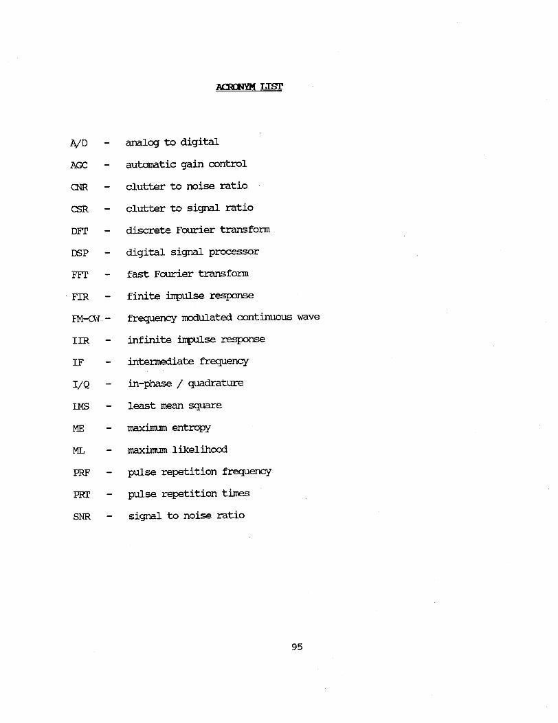
ACIHNYM isr
A/D - analog to digital
AGC - automatic gain control
CNR - clutter to noise ratio
CSR - clutter to signal ratio
DFT - discrete Fourier transform
DSP - digital signal processor
FFT - fast Fourier transform
FIR - finite impulse response
FM-CW - frequency modulated continuous wave
IIR - infinite impulse response
IF - intermediate frequency
I/Q - in-phase / quadrature
IMS - least mean square
ME - maximum entropy
ML - maximum likelihood
PRF - pulse repetition frequency
PRT - pulse repetition times
SNR - signal to noise ratio
95


B I B L T OQ"A B I Y
Alexander, S.T., 1986a: Adaptive Signal Processing: Theory andApplications. New York: Springer Verlag.
_______, 1986b: Fast adaptive filters: A geometric approach.IEEE Trans. Acoust., Speech, and Sig. Proc., 3, No. 4, 18-20.
Aliphas, A., and J.A. Feldman, 1987: The versatility of digital signalprocessing chips. IEEE Spetru, 24, No. 6, 40-45.
Alldritt, M., R. Jones, C.J. Oliver, and J.M. Vaughan, 1978: The processingof digital signals by a surface acoustic wave spectrum analyzer. J.Phys. E: Sci. Instrum., 11, 116-119.
Allen, J., 1985: Computer architecture for digital signal processing.Proc. IEEE, 73, No. 5, 852-873.
Anderson, C.M., E.H. Satorius, and J.R. Zeidler, 1983: Adaptive enhancementof finite bandwidth signals in white Gaussian noise. IEEE Trans.Acoust., Speech, and Sig. Proc., ASSP-31, No. 1, 17-28.
Anderson, J.R., 1981: Evaluating ground clutter filters for weather radars.Preprints 20th Conf. Radar Meteor., AMS, 314-318.
, 1987: The measurement of Doppler wind fields with fastscanning radars: signal processing techniques. J. Atmos. Ocean.Tech., 4, no. 4, 627-633.
Anderson, N., 1978: Comments on the performance of maximum entropyalgorithms. Proc. IEE, 66, 1581-1582.
Aoyagi, J., 1983: A study on the MTI weather radar system for rejectingground clutter. Papers in Meteorology and Geophysics, 33, 187-243.
Applebaum, S.P., 1976: Adaptive arrays. IEEE Trans. Antennas Propaqat.,AP-24, 585-598 (Special issue on Adaptive Antennas).
Atlas, D., 1964: Advances in radar meteorology. Advances in Geophysics,10, Landsberg and Mieghem, Eds. New York: Academic, 317-478.
Atlas, D. and R.K. Moore, 1987: The measurement of precipitation withsynthetic aperture radar. J. Atmos. Ocean. Tech., 4, 368-376.
Austin, G.L., 1974: Pulse compression systems for use with meteorologicalradars. Radio Science, 9, No. 1, 29-33.
Baggeroer, A.B., 1976: Confidence intervals for regression MEM Spectralanalysis, IEEE Trans. Inform. Theory, IT-22, 534- 545.
97

Balsley, B.B., and R.F. Woodman, 1969: On the control of the F-regionelectric field: experimental evidence. J. Atmos. Terrest. Phys., 31,865-867.
Bargen, D.W. and R.C. Brown, 1980: Interactive radar velocityunfolding. Preprints 19th Conf. Radar Meteor., AMS, Boston, 278-285.
Barton, D.K., 1975: Radars, Vol. 3. Pulse Compression. Dedham, MA: ArtechRadar Library.
, and H.R. Ward, 1984: Handbook of RadarMeasurement, Dedham,MA: Artech House.
Battan, L.J., 1973: Radar Observation of the Atmosphere, Chicago:University of Chicago Press.
Bello, P.A., 1965: Some techniques for the instantaneousmeasurement of multipath and Doppler spread. IE:E TransTech., COM-13, No. 3, 185-292.
Benham, F.C., H.L. Groginsky, A.S. Soltes, and G. Works, 1972:estimation of Doppler spectrum parameters. Final Report,19628-71-C-0126, Raytheon Company, Wayland, Mass.
Bergen, W.R., and S.C. Albers, 1988:of Doppler radar velocities.319.
real-timeon Comm.
Pulse pairContract F-
Two and three dimensional de-aliasingJ. Atmos. Ocean. Tech., 5, No. 2, 305-
Berger, T., and H.L. Groginsky, 1973: Estimation of the spectral moments ofpulse trains. Paper presented at the Int. Conf. on Information Theory,Tel Aviv, Israel.
Bilbro, J.G., D. Fichtl, D. Fitzjarrald, M. Krause andAirborne Doppler lidar wind field measurements. Bull.Soc., 65, 348-359.
R. Lee, 1984:Amer. Meteor.
, C. DiMarzio, D. Fitzjarrald, S. Johnson, and W. Jones, 1986:Airborne Doppler lidar measurements. Appl. Opt., 25, 3952.
Blackman, R.B., and J.W. Tukey, 1958: The Measurement of Power Spectra.New York: Dover.
Bode, H.W., and C.E. Shannon, 1950: A simplified derivation of linear leastsquares smoothing and prediction theory. Proc. IRE, 38, 417-425.
Boren, T.A., J.R. Cruz,approach to DopplerConf. Radar Meteor.,
and D. Zrnic, 1986:weather radar velocity
AMS, JP107-110.
An artificial intelligencede-aliasing. Preprints 23rd
Bracewell, R., 1965: The Fourier Transform and Its Applications. New York:McGraw-Hill.
98
9
Bringi, V.N., T.A. Seliga and S.M. Cherry, 1983: Statistical properties ofthe dual polarization differential reflectivity (ZDR) radar signal.IEEE Trans. Geosci. Remote Sens., GE-21, 215-220.
, and A. Hendry, 1988: This volume, Chapter 19A.
Brookner, E., 1977: Radar Technology. Dedham, MA: Artech House.
Browning, K.A., P.K. James, D.M. Parkes, C. Rowley, and A.J. Whyman, 1978:Observations of strong wind shear using pulse compression radar.Nature, 271, 529 - 531.
Burg, J.P., 1967: Maximum entropy spectral analysis. 37th Annual Intl. Soc.Exploration Geophysicists Meeting, Oklahoma City, OK, Oct. 31.
, 1968: A new analysis technique for time series data.NATO Advanced Study Institute on Signal Processing with Emphasis onUnderwater Acoustics Vol 1, paper #15, Enschede, Nederlands.
, 1972: The relationship between maximum entropy spectra andmaximum likelihood spectra. Geophysics, 37, No. 2, 375-376.
, 1975: Maximum entropy spectral analysis. Ph.D. Dissertation,Dept. of Geophysics, Stanford University.
Cadzow, J.A., 1980: High performance spectral estimation -- a new ARMAmethod. IEEE Trans. Acoust., Speech, Signal Processing, ASSP-28, No.5, 524-529.
, 1982: Spectral estimation: An overdetermined rational modelequation approach. Proc. IEEE, 70, No. 9, 907-939 (Special issue onSpectral Estimation).
Campbell, W.C., and R.C. Strauch, 1976: Meteorological Doppler radar withdouble pulse transmission. Preprints, 17th Conf. Radar Meteor., AMS,42-44.
Capon, J., 1969: High-resolution frequency-wavenmber spectrum analysis.Proc. IEEE 5,7, 1408-1418.
Caton, P.A.F., 1963: Wind measurement by Doppler radar. Meteor. Mag., 92,213-222.
Chadwick, R.B., and G.R. Cooper, 1972: Measurement of distributed targetswith the random signal radar. IEEE Trans. on Aerosp. Electron. Syst.,AES-8, 743-750.
, K.P. Moran, R.G. Strauch, G.E. Morrison, and W.C. Campbell,1976: Microwave radar wind measurements in the clear air. RadioScience, 11, No. 10, 795-802.
99

, and R.G. Strauch, 1979:signals from distributed targets.Sys., AES-15, 185-188.
Processing of FM-CW Doppler radarIEEE Trans. on Aerosp. Electron.
Chakrabarti, N., and M. Tomlinson, 1976: Design of sequences with specifiedautocorrelation and cross correlation. IEEE: Trans. on Communications,COM-24.
Chandra, M., T. Jank,Ritenberg, 1986:Preurints 23rd Conf.
P. Meischner, A. Schroth, E. Clemens, and F.The advanced coherent polarimetric DFVLR radar.Radar Meteor., AMS, JP385-393.
Chandrasekar, V., G.R. Gray, V.N. Bringi, and R.J. Keeler, 1989:Efficient differential reflectivity processing usingreceivers. J. Atmos. Ocean. Tech., 6, in press.
logarithmic
Childers, D.G., 1978: Modern Spectrum Analysis.Reprint Series, New York: I:F Press.
IEEE Press Selected
Chimera, A.M., 1960: Meteorological radar echo study. Cornell Aero Labs,Buffalo, N.Y., Final Rep. Contract AF33(616)-6352.
Adaptive Antennas. Englewood Cliffs, N.J.: Prentice
Cook, C.E., 1960: Pulse compression:transmission. Proc. IRE, 48, 310-316.
, and M. Bernfeld, 1967: Radar Signals:Theory and Application. New York: McGraw-Hill.
Cooley, J.W., and J.W. Tukey, 1965:calculation of complex Fourier series.
Key to more efficient radar
An Introduction to
An algorithm for the machineMath Camp, 19, 297- 301.
Costas, J.P., 1984: A study of a class of detection waveformsideal range-Doppler ambiguity properties. Proc. IEE,996-1009.
having nearly72, No. 8,
Crane, R.K., 1980: Radar measurements of wind at Kwajalein. Radio Science,15, No. 2, 383-394.
Davenport, W.B., and W.L. Root, 1958: An Introduction to the Theory ofRandom Signals and Noise. New York: McGraw-Hill.
Dazhang, T., S.G. Geotis, R.E. Passarelli, Jr., A.L. Hansen, and C.L. Frush,1984: Evaluation of an alternating PRF method for extending the rangeof unambiguous Doppler velocity. Preprints 22nd Conf. Radar Meteor.,AMS, 523-527.
Deley, G.W., 1970: Waveform design. Radar Handbook, Merril I. Skolnik, Ed.New York: McGraw-Hill 3.1-3.47.
100
Compton, R.T., 1988:Hall.
-6 J. P.1 .4 a .4.,A........ b
--I

Denenberg, J.N., 1971: The estimation of spectral moments. Report of Lab.Atmos. Probing, Dep. Geophys. Sci., Univ. Chicago and Dep. Elect. Eng.,Illinois Inst. Tech.
_______ , 1976: Spectral moment estimators: A new approach to tonedetection. The Bell System Technical Journal, 55, No. 2, 143-155.
, R.J. Serafin, and L.C. Peach, 1972: Uncertainties incoherent measurement of the mean frequency and variance of the Dopplerspectrum from meteorological echoes. Preprints 15th Conf. RadarMeteor., AMS, 216-221.
Doviak, R.J., and D.S. Sirmans, 1973: Doppler radar with polarizationdiversity. J. Atmos. Sci., 30, 737-738.
, D. Sirmans, D. Zrnic, and G.B. Walker, 1978: Considerationsfor pulse-Doppler radar observations of severe thunderstorms. J. Appl.Met., 17, No. 2, 189-205.
, D.S. Zrnic, and D.S. Sirmans, 1979: Doppler weather radar.Proc. IFFE, 67, No. 11, 1522-1553.
, R.M. Rabin, and A.J. Koscielny, 1983: Doppler weather radarfor profiling and mapping winds in the prestorm environment. IEEETrans. Geosci. Remote Sens., GE-21, No. 1, 25-33.
, and D.S. Zrnic, 1984: Doppler Radar and Weather Observations,New York: Academic Press.
Evans, J.E., 1983: Ground Clutter cancellation for the NEXRAD system.Lincoln Laboratory project report ATC-122, Mass. I n s t i t u t e o fTechnology.
Farina, A., editor, 1987: Optimised Radar Processors. London, PeterPeregrinus Ltd.
Farley, D.T., 1969: "Incoherent scatter correlation function measurements."Radio Science, 4, No. 10, 935-953.
Fetter, R.W., 1970: Radar weather performance enhanced by pulsecompression. Preprints 14th Conf. Radar Meteor., AMS, 413- 418.
, 1975: Real time analog Doppler processing (RANDOP).Preprints 16th Conf. Radar Meteor., AMS, 153-555.
Fischler, M.A., and R.C. Bolles, 1981: Random sample consensus: A paradigmfor model fitting with applications to image analysis and automatedcartography. Commun. of ACM, 24, 381-395.
Foord, R., R. Jones, J.M. Vaughan, and D.V. Willetts, 1983: Precise
101
comparison of experimental and theoretical SNR's in C02 laserheterodyne systems. Appl. Opt., 23, 3787.
Frank, R.L., 1963: Polyphase codes with good nonperiodic correlationproperties. IEEE Trans. on Information. Theory, IT-9, 43-45.
Friedlander, B., 1982: Lattice methods for spectral estimation. Proc.IEEE, 70, 990-1017 (Special issue on Spectral Estimation).
Frush, C.L., 1981: Doppler signal processing using IF limiting. Preprints20th Conf. Radar Meteor., AMS, 332-336.
Gabriel, W.F., 1976: Adaptive arrays - an introduction. Proc. IEE, 64,239-272.
, 1980: Nonlinear spectral analysis and adaptive array superresolution techniques. NRL Report 8345, reprinted in Lewis,Kretschwer, & Shelton (1986) Aspects of Radar Signal Processing,Harwood, MA: Artech House.
Gage, K.S., and B.B. Balsley, 1978: Doppler radar probing of the clearatmosphere. Bulletin AMS, 59, No. 9, 1074-1093.
_, 1988: This volume, Chapter 28A.
Geotis, S.G. and W.M. Silver, 1976: An evaluation of techniques forautomatic ground echo rejection. Preprints 17th Conf. Radar Meteor.,AMS, 448-452.
Glover, K.M., G.M. Armstrong, A.W. Bishop and K.J. Banis, 1981: A dualfrequency 10 cm Doppler weather radar. Preprints 20th Conf. RadarMeteor., AMS, 738-743.
Golay, M.J.E., 1961: Complementary series. IRE Trans. Info. Theory, IT-7,82-87.
Gold, B., and C.M. Rader, 1969: Digital Processing of Signals, New York:McGraw-Hill.
Gonzales, C.A., and R.F. Woodman, 1984: Pulse compression techniques withapplication of HF probing of the mesosphere. Radio Science, 19, No. 3,871-877.
Gossard, E.E., and R.G. Strauch, 1983: Radar Observations of Clear Air andClouds. New York: Elsevier Science Publishers B.V.
Gray, G.R., R.J. Serafin, D. Atlas, R.E. Rinehart, and J. Boyajian, 1975:Real time color doppler radar display. Bulletin AMS, 56, no. 6, 580-588.
Gray, R.W., and D.T. Farley, 1973: Theory of incoherent scattermeasurements using compressed pulses. Radio Science, 8, 123-131.
102

Griffiths, L.J., 1975: Rapid measurement of digital instantaneousfrequency. IEEE Trans. on Acoustics, Speech and Signal Processing,ASSP-23, 207-222.
Groginsky, H.L., 1965: The coherent memory filter. Electron. Prog., 9, No.3, 7-13.
, 1966: Digital processing of the spectra of pulse Dopplerradar precipitation echoes. Preprints 12th Conf. Radar Meteor., AMS,34-43.
, 1972: Pulse pair estimation of Doppler spectrumparameters. Preprints 15th Conf. Radar Meteor., AMS, 233-236.
, A. Soltes, G. Works, and F.C. Benham, 1972: Pulse pairestimation of Doppler spectrum parameters. Final Report, [NTIS AD744094], Raytheon Company, Wayland, MA. 158.
, and K.M. Glover, 1980: Weather radar canceller design.Preprints 19th Conf. Radar Meteor., AMS, 192-198.
Hamidi, S., and D.S. Zrnic, 1981: Considerations for the design of groundclutter cancelers for weather radars. Preprints 20th Conf. RadarMeteor., AMS, 319-326.
Hansen, D.S., 1985: Receiver and analog homodyning effects on Dopplervelocity estimates. J. A. Atmos. Ocean. Tech., 2, 644-655.
Hardesty, R.M., 1986: Performance of a discrete spectral peak frequencyestimator for Doppler wind velocity measurements. IEEE Trans. Geosci.Remote Sens., GE-24, No. 5, 777-783.
_____ _ , R.E. Cupp, M.J. Post, and T.R. Lawrence, 1988: A ground-based, injection-locked, pulsed TEA laser for atmospheric windmeasurements. Proc. SPIE , 889, 23-28.
Hardy, K.R., and I. Katz, 1969: Probing the clear atmosphere with highpower, high resolution radars. Proc. IEEE, 57, No. 4, 468-480.
Harris, F.J., 1978: On the use of windows for harmonic analysis with theDiscrete Fourier Transform. Proc. IEEE, 66, No. 1, 51-83.
Haykin, S., 1982: Maximum-entropy spectral analysis of radar clutter.Proc. IEEE, 70, No. 9, 953-962.
, 1983: Communication Systems. New York: John Wiley & Sons.
, editor, 1985a: Array signal processing. Englewood Cliffs, NJ:Prentice Hall.
103

, 1985b: Radar signal processing. IEEE Trans. on Acoustics,Speech & Signal Processing, ASSP-33, 2-18.
, 1986: Adaptive Filter Theory. Englewood Cliffs, NJ: PrenticeHall.
____ , and S. Kesler, 1976: The crmplex form of the maximum entropymethod for spectra estimation. Proc. ITEE, 64, 822-823.
, and J.A. Cadzow, 1982: Scanning the issue - The special issueon spectral estimation. Proc. IEEE, 70, No. 9, 883-884.
, B.W. Currie, and S.B. Kesler, 1982: Maximum-entropy spectralanalysis of radar clutter. Proc. IEEE, 70, 953-962 (Special issue onSpectral Estimation).
Heideman, M.T., D.H. Johnson, and C.S. Burrus, 1984: Gauss and the historyof the fast fourier transform. IEEE Trans. on Acoustics, Speech &Signal Processing, ASSP-32, 14-21.
Hennington, Larry, 1981: Reducing the effects of Doppler Radar Ambiguities.J. Appl. Met., 20, 1543-1546.
Hildebrand, P.H., and R.S. Sekhon, 1974: Objective determination of noiselevel in Doppler spectra. J. Appl. Met., 13, 808-811.
, and R.K. Moore, 1988: This volume, Chapter 22A.
Hjelmfelt, M.R., A.J. Heymsfield and R.J. Serafin, 1981: Combined radar andaircraft analysis of a Doppler radar "black hole" region in an Oklahomathunderstorm. Preprints 20th Conf. Radar Meteor., AMS, Boston, 66-70.
Honig, M.L., and D.G. Messerschmitt, 1984: Adaptive Filters: Structures,Algorithms, and Applications. Boston: Kluwer Academic Publishers.
Howells, P.W., 1976: Explorations in fixed and adaptive resolution at GEand SURC. IEEE Trans. on Antenna Prep., AP-24, 575-584 (Special issueon Adaptive Antennas).
Huffaker, R.M., 1974-75: C02 laser Doppler systems for the measurement ofatmospheric winds and turbulence. Atmospheric Technology, NCAR, 71.
, D.W. Beran, and C.G. Little, 1976: Pulsed coherent lidarsystems for airborne and satellite based wind field measurement. Proc.7th Conf. Aerosp and Aeronaut. Meteor., AMS, 318-324.
,_ T.R. Lawrence, M.J. Post, J.T. Priestley, F.F. Hall, Jr.,R.A. Richter, and R.J. Keeler, 1984: Feasibility studies for a globalwind measuring satellite system (Windsat): Analysis of simulatedperformance. Appl. Opt., 23, 2523-2536.
104

Hyde, G.H., and K.E. Perry 1958:Tech. Rep., TR no.189.
Doppler phase difference integrator. MIT
Jackson, L.B., J.F. KimplementationElectroacoustics,
aiser, and H.S. McDonald, :of digital filters.ASSP-17, No. 2, 104-108.
1969: An approach to theIEEE Trans. Audio and
Janssen, L.H. and Van der Spek, 1985:precipitation. IF:E Trans. Aerosp.
The shape of Doppler spectra fromElectron. Syst., AES-21, 208-219.
Jaynes, E.T., 1982: On the rationale of maximum-entropy methods. Proc.IEEE, 70, 939-952 (Special issue on Spectral Estimation).
Jelalian, A.V., 1977: Laser Radar Theory and Technology. Chapter 24. E.Brookner, Ed. Artech House.
, 1980: Laser radar systems. RecorAerospace Systems Cony. (EASOON), Arlington, VA.
d IEEE Electronics and
, 1981a: Laser and microwave radar. Laser Focus, 88-94.
, 1981b: Laser radar improvements. IEEE Spectrum, 18, 46-51.
Jenkins, G.M. and D.G. Watts, 1968: Spectral Analysis and Its Applications.San Francisco: Holden-Day.
Kailath, T., 1974: A view of three decades of linear filtering theory.IEEE Trans. Inf. Theory, IT-20, 146-181.
Kaiser, J.F., 1966: Digital filters. Chap. 7 Systems Analysis by DigitalComputer, F.F. Kuo & J.F. Kaiser (eds.), New York: Wiley.
Kay, S.M., 1987:Prentice Hall.
Modern Spectral Estimation. Englewood Cliffs, N.J.:
Kay, S., and L. Marple, 1981: Spectrum analysis - A modern perspective.Proc. I F, 69, No. 11, 1380-1419.
Keeler, R.J., 1978: Uncertainties in adaptive maximum entropy frequencyestimators. IEEE Trans. on Acoustics, Speech and Signal Proc., ASSP-26, no. 5, 469-471.
, and L.J. Griffiths, 1977: Acouadaptive linear prediction filtering. J.1227.
, and R.W. Lee, 1978: ComplexDoppler estimates for pulsed O02 lidar.Conf. on Acoustics, Speech and Sicnal Proc.
istic Doppler extraction byAcoust. Soc. Am., 61, 1218-
covariance/maximum entropyProceedings of IEEE Intl.
, Tulsa, OK. 365-368.
and C.L. Frush, 1983a: Coherent wideband processing of
105
��- -�- I
distributed radar targets. Digest of Int'l. Geoscience and RemoteSensing Symposium (IGARSS-83), San Francisco, PS1 (3.1 - 3.5).
_, 1983b: Rapid scan doppler radar developmentconsiderations. Preprints 21st Conf. Radar Meteor., AMS, 284-290.
, and R.E. Carbone, 1986:for meterological Doppler radars.AMS, 357-360.
A modern pulsing/processing techniquePreprints 23rd Conf. Radar Meteor.,
Kesler, S.B., 1986: Modern Spectrum Analysis, II. Drexel University, IEEEPress.
Khinchine, A.J., 1934:processes. Math. Ann.,
Correlation theory of stationary stochastic109, 604-15.
Klauder, J.R., A.C. Price, S. Darlington, and W.J. Albersheim, 1960:theory and design of chirp radars. Bell System Technical Journal,745-808.
Klostermeyer, J., 1986:likelihood spectra of731-736.
Experiments with maximum entropy and maximumVHF radar signals. Radio Science, 21, No. 4,
Krehbiel, P.R., and M. Brook, 1968: The fluctuating radar echo. Proc. 13thWeather Radar Conf., AMS, Boston, 2-11.
, 1979: A broad-band noise technique for fast-scanning radar observations of clouds and clutter targets. IEEE Trans.on Geoscience Electronics, GE-17, 196-204.
Kretschmer,codedSyst.,
F.F. Jr., and B.L. Lewis, 1983: Doppler properties of polyphasepulse compression waveforms. IEEE Trans.on Aerosp. Electron.AES-19, .No. 4, 521-531.
Lacoss, R.T., 1971:36, 661-675.
Data adaptive spectral analysis methods. Geophysics,
Laird, B.G., 1981: On ambiguity resolution by random phase processing.Preprints 20th Conf. Radar Meteorology, AMS, 327-331.
Lang, S.W., and J.H. McClellan, 1980: Frequency estimation with maximumentropy spectral estimators. IEEE Trans. Acoust., Speech, and Sig.Proc., ASSP-28, 716-724.
Lawrence, T.R., D.J. Wilson, M.C.velocimeter for remote windPreprints of Intl. Conf on Ae:Washington, D.C., AMS, 317-320.
Krause, 1972: Application of a laservelocity and turbulence measurements.rosp. and Aeron. Met. Mav 22-26, 1972,
Lee, R.W., 1978: Performance of the poly-pulse-pair Doppler estimator.Lassen Res. Memo 78-03.
106
The39,
. - r r

, and K.A. Lee, 1980: A poly-pulse-pair signal processor forcoherent Doppler lidar. Digest of OSA Topical Meeting on coherentlaser radar for atmospheric sensing, WA2-4, Aspen, Colorado.
Levin, M.J., 1965: Power spectrum parameter estimation. IEEE Trans. Inform.Theory, IT-11, 100-107.
Lewis, B.L., F.F. Kretschmer, Jr., and W.W. Shelton, 1986: Aspects of RadarSignal Processors, Norwood, MA: Artech House.
Ihermitte, R.M., 1960: The use of special "pulse Doppler radar" inmeasurements of particle fall velocities. Proc. 8th Wea. Radar Conf.,269-275.
, 1972: Real time processing of meteorological Doppler radarsignals. Preprints 15th Conf. Radar Meteor., AMS, 364-367.
, and D. Atlas, 1961: Precipitation motion by pulse Dopplerradar. Proc. 9th Conf. Weather Radar, AMS, 218-223.
, and R. Serafin, 1984: Pulse-to-pulse coherent Dopplersonar signal processing techniques. J. Atmos. Ocean. Tech., 1, No. 4,293-308.
Li, F.K., K.E. Im, W.D. Wilson, and C. Blachi, 1987: On the design issuesfor a spaceborne rain mapping radar. Proc. Internat. Symposium onTropical Precipitation Measurements, Tokyo, Oct. 1987. A. DeepakPublishing (in press).
Ligthart, L.P., L.R. Nieuwkerk, and J. van Sinttruyen, 1984: FM-CW Dopplerradar signal processing for precipitation measurements. Preprints 22ndConf. Radar Meteor., AMS, 538-543.
Lippmann, R.P., 1987: An introduction to computing with neural nets. IEEEAcoustics, Speech and Signal Processing Magazine, 4, No. 2, 4-22.
Little, C.G., 1969: Acoustic methods for the remote probing of the loweratmosphere. Proc. I:TEEE, 57, No. 4, 571-578 (Special issue on RemoteEnvironmental Sensing).
Mahapatra, P.R., and D.S. Zrnic, 1983: Practical algorithms for meanvelocity estimation in pulse Doppler weather radars using a smallnumber of samples. IEEE Trans. Geosci. Remote Sens., GE-21, 491-501.
Mailloux, R.J., 1982: Phased array theory and technology. Proc. IEEE, 70,246-291.
Makhoul, J., 1975: Linear prediction: A tutorial review. Proc. IEEE, 63,561-580 (Special issue on Digital Signal Processing). Correction inProc. IEEE, 64, 285, 1976.
107

, 1977: Stable and efficient lattice methods for linearprediction. IEEE Trans on Acoustics, Speech and Signal Proc., ASSP-25,423-428.
, 1986: Maximum confusion spectral analysis. IEEE Third ASSPWorkshop on Spectrum Estimation and Modeling, Boston, 6-9.
Marple, S.L., 1987: Digital Spectral Analysis with Applications, Prentice-Hall, Englewood Cliffs, N.J.
Marshall, J.S., 1971: Peak reading and thresholding in processing radarweather data. J. Appl. Meteor., 10, 1213-1223.
, and W. Hitschfeld, 1953: Interpretation of thefluctuating echo from randomly distributed scatters (Part I). Can.Jour. Phys., 31, Pt. 1, 962-995.
McCaul, E.W. Jr., H.B. Bluestein, and R.J. Doviak, 1986: Airborne Dopplerlidar techniques for observing severe thunderstorms. Appl. Optics, 25,No. 5, 698-708.
McClellan, J.H., 1982: Multidimensional spectral estimation. Proc. IEEE70, 1029-1039 (Special issue on Spectral Estimation).
McWhirter, J.G., and E.R. Pike, 1978: The extraction of information fromlaser anemometry data. Physica Scripta, 119, 417-425.
Merritt, M.W., 1984: Automatic velocity de-aliasing for real-timeapplications. Preprints 22nd Conf. Radar Meteor., AMS., 528-533.
Miller, K.S., 1970: Estimation of spectral moments of time series.Biometrika, 57, 513-517.
, and M.M. Rochwarger, 1970: On estimating spectral moments inthe presence of colored noise. IEEE Trans. Inform. Theory, IT-16, 303-309.
, 1972: A covariance approach to spectralmoment estimation. IEEE Trans. Inform. Th., IT-18, No. 5, 588-596.
Miller, K.W., 1979: Estimation of Doppler centroid of fading radar targets.IEEE Trans. Aerosp. Electron. Syst., AES-15, No. 1, 171-177.
Miller, R.W., 1972: Techniques for power spectrum moment estimation. Proc.Int. Conf. Communications, 45.23-45.27.
Mitchell, R.L., 1976: Radar Signal Simulation. Dedham, MA: Artech House.
Monzingo, R.A., and T.W. Miller, 1980: Introduction to Adaptive Arrays.New York: Wiley & Sons.
108

Morf, M., A. Vieira, D.T. Lee, and T. Kailath, 1978: Recursive multichannelmaximum entropy spectral estimation. IEEE Trans. on GeoscienceElectronics, GE-16, 85-94.
Mueller, E.A., and E.J. Silha, 1978: Unique features of the CHILL radarsystem. Preprints 18th Conf. Radar Meteor., 381-382.
Nathanson, F.E., 1969: Radar Design Principles, New York: McGraw-Hill.
, and J.P. Reilly, 1968: Radar Precipitation Echoes. IEEETrans. Aerosp. Electron. Syst., AES-4, No. 4, 505-514.
Novak, L.M. and N.E. Lindgren, 1982: Maximum likelihood estimation ofspectral parameters using burst waveforms. Proc. 16th Asilomar Conf.on Circuits, Systems and Computers, IEE Computer Society Press, NewYork, 318-324.
Nyquist, H., 1928: Certain topics in telegraph transmission theory. AIEETrans, 47, 617-644.
Oliver, C.J., 1979: Pulse compression in optical radar. IEEE Trans.Aerosp. Electron. Syst., AES-15, No. 3., 306-324.
Oppenheim, A.V., and R. W. Schafer, 1975: Digital Signal Processing,Englewood Cliffs, N.J.: Prentice-Hall.
Paczowski, H.C., and J. Whelehan, 1988: Understanding Noise: Part I andII. IEEE MITS-Newsletter. Winter, 23-36.
Papoulis, A., 1962: The Fourier Integral and Its Applications. New York:McGraw-Hill.
, 1981: Maximum entropy and spectral estimation: a review.IEEE Trans. on Acoustics, Speech and Signal Processing, ASSP-29, No. 6,1176-1981.
, 1965 and 1984: Probability, Random Variables, and StochasticProcesses. New York: McGraw-Hill.
Parzen, E., 1957: On consistent estimates of the spectrum of a stationarytime series. Ann. Math. Stat., 28, 329-348.
Passarelli, R.E., 1981: Autocorrelation techniques for ground clutterrejection. Preprints 20th Conf. Radar Meteor., AMS, 308-313.
, 1983: Parametric estimation of Doppler spectral moments:An alternative ground clutter rejection technique. J. Clim. and Appl.Met., 22, 850-857.
, P. Romanik, S.G. Geotis, and A.D. Siggia, 1981: Groundclutter rejection in the frequency domain. Preprints 20th Conf. RadarMeteor., AMS, Boston, 295-300.
109

, and A.D. Siggia, 1983: The autocorrelation function andDoppler spectral moments: Geometric and asymptotic interpretation.Jour. Climate and Appl. Meteorology, 22, No. 10, 1776-1787.
, R.J. Serafin, and R. Strauch, 1984: Effects of aliasingon spectral moment estimates derived from the complex autocorrelationfunction. J. Climate Appl. Meteorol., 23, 848-849.
Probert-Jones, J.R.,Royal Met. Soc.,
1962: The radar equation in meteorology. Quart J.88, 485-495.
Rabiner, L.R., and B. Gold, 1975: Theory and Application of Digital SignalProcessing. Englewood Cliffs, N.J.: Prentice-Hall.
Rabinowitz,1985:No. 2,
S.J., C.H. Gager, E. Brookner, C.E. Muehe, and C.M. Johnson,Applications of digital technology to radar. Proc. IEE, 73,325-339 (Special issue on Radar).
Rader, C.M., 1984: A simple method for sampling in-phase and quadraturecomponents. IEEE Trans. on Aerospace and Electronic Systems, AES-20,No. 6, 821-824.
Radoski, H.R., P.F. Fougere, and E.J. Zawalick, 1975: A comparison of powerspectral estimates and applications of the maximum entropy method. J.of Geophysical Research, 80: 619-625.
Rastogi, P.K.,Jicamarca1217-1231.
and R.F. Woodman, 1974: Mesospheric studies using theincoherent-scatter radar. J. Atmos. Terrestrial Phys., 36,
Ray, P.S., and C. Ziegler, 1977:estimates. J. Appl. Met., 16, 563-564
De-aliasing first-moment Doppler
Reid, M.S., 1969: A millimeter wave pseudorandom coded meteorologicalradar. IEEE Trans. Geosci. Electron., GE-7, No. 3, 146-156.
Richter, J. H., 1969: High resolution tropospheric radar sounding.Science, 4, 1261-1268.
Radio
Rife, D.C., and R.R. Boorstyn, 1974: Single tone parameter estimation fromdiscrete-time observation. IEEE Trans. on Info. Theory, IT-20, No. 5,591-598.
Rihaczek, A.W., 1969:McGraw-Hill.
Principles of high resolution radar, New York:
Roberts, R.A., and C.T. Mullis, 1987: Digital Signal Processing. Reading,MA: Addison-Wesley.
110

Robinson, E.A., 1982: A historical perspective of spectrum estimation.Proc. IEEE, 70, 885-907 (Special issue on Spectral Estimation).
Rogers, R.R., 1971: The effect of variable target reflectivity on weatherradar measurements. Quart. J. Royal. Met. Soc., 97, 154-167.
_____ , and A.J. Chimera, 1960: Doppler spectra from meteorologicalradar targets. Proc. 8th Weather Radar Conf., 377-385.
Rottger, J., and M. Larsen, 1988: This volume, Chapter 21A.
, J. Klostermeyer, P. Czechowsky, R. Ruister, and G. Schmidt,1978: Remote sensing of the atmosphere by VHF radar experiments.Naturwissenschaften, 65, 285-296.
Rummler, W.D., 1968a: Introduction of a new estimator for velocity spectralparameters. Tech. memo. MM-68-4121-5, Bell Labs, Whippany, N.J.
, 1968b: Accuracy of spectral width estimators using pulsepair waveforms. Tech. memo. MM-68-4121-14, Bell Labs, Whippany, N.J.
, 1968c: Two pulse spectral measurements. Tech. memo MM-68-4121-15, Bell Labs, Whippany, N.J.
Rutkowski, W., and A. Fleisher, 1955: R-meter: An instrument for measuringgustiness. M.I.T. Weather Radar Res. Rep., 24.
Sachidananda, M., and D.S. Zrnic, 1985: ZDR measurement considerations fora fast scan capability radar. Radio Science, 20, No. 4, 907-922.
, R.J. Doviak, and D.S. Zrnic, 1985: Whitening of sidelobepowers by pattern switching in radar array antenna. IEEE Trans. onAnt. and Prop., AP-33, No. 7, 727-735.
____-, 1986: Recovery of spectral moments fromoverlaid echoes in a Doppler weather radar. IEEE Trans. on Geosci.Remote Sens., GE-24, No. 5, 751-764.
, 1989: Efficient processing of alternatelypolarized radar signals. J. Atmos. Ocean. Tech., 6, in press.
Sato, T., and R.F. Woodman, 1982: Spectral parameter estimation of CATradar echoes in the presence of fading clutter. Radio Science, 17, No.4, 817-826.
Sawate, D.V., and M.B. Dursley, 1980: Crosscorrelation properties ofpseudo-random and related sequences. Proc. IEEE, 68, No. 5, 593-619.
Schmidt, G., R. Rister, and P. Czechowsky, 1979: Complementary code anddigital filtering for detection of weak VHF radar signals from themesosphere. IEEE Trans. on Geoscience Electronics, GE-17, No. 4, 154-161.
111
Schnabl, G., M. Chandra, A. Schroth, and E. Luneburg, 1986: The advancedpolarimetric DFVLR radar: First measurements and its unique signal-processing and calibration aspects. Preprints 23rd Conf. RadarMeteor., 1, 159-164.
Schriver, B.D., 1988: Artificial neural systems. IEE::: Computer, 21, No. 3,8-9 (Special issue on neural networks).
Schroth, A.C., M.S. Chandra, and P.S. Meischner, 1988: C-band coherentpolarimetric radar for propagation and cloud physics research. J.Atmos. Ocean. Tech., 5, 803-822.
Serafin, R.J., and R.G. Strauch, 1978: Meteorological radar signalprocessing. Air Quality Meteorology and Atmospheric Ozone. A. L.Morris and R.C. Barras (Eds.), Amer. Soc. for Testing and Materials,159-182.
Shannon, C.E., 1949: Communication in the presence of noise. Proc. IRE,37, 10-21.
Shirakawa, M. and D.S. Zrnic, 1983: The probability density of a maximumlikelihood mean frequency estimator. IEEE Trans. on Acoustics, Speechand Signal Processing, ASSP-31, No. 5, 1197-1201.
Sibul, L.H., 1987: Adaptive Signal Processing. Penn. State Univ.: IEEPress.
Siggia, A.D., 1981: A real-time Doppler spectrum analyzer. Preprints 20thConf. Radar Meteor., AMS, 222-227.
, 1983: Processing phase coded radar signals with adaptivedigital filters. Preprints 21st Conf. Radar Meteor., AMS, 167-172.
Sirmans, D., 1975: Estimation of spectral density mean and variance bycovariance argument techniques. Preprints 16th Conf. Radar Meteor.,AMS, 6-13.
, and R.J. Doviak, 1973: Meteorological radar signal intensityestimation. NOAA Tech memo ERL-NSSL-64, 69-71.
, and B. Bumarner, 1975a: Estimation of spectral density meanand variance by covariance argument techniques. Preprints 16th Conf.Radar Meteor., AMS, 6-13.
, 1975b: Numerical comparison of five meanfrequency estimators. J. Appl. Meteor., 14, 991-1003.
, D. Zrnic, and B. Bumgarner, 1976: Extension of maximumunambiguous Doppler velocity by use of two sampling rates. Preprints17th Conf. Radar Meteor., AMS, 23-28.
112

, and J.T. Dooley, 1980: Ground clutter statistics of a 10 cnground based radar. Preprints 19th Conf. Radar Meteor., AMS, 184-191.
Skolnik, M.I., 1970: Radar Handbook. New York: McGraw-Hill.
, 1980: Introduction to Radar Systems.Hill.
New York: McGraw-
Smith, P.L., 1987:Doppler spectralOcean. Tech., 4,
The relationship between coherentprocessing of weather radar echoes.541-544.
integration andJ. Atmos. and
, 1986: On the sensitivity of weather radars. J. Atmos. Ocean.Tech., 3, No. 4, 704-713.
, K.R. Hardy, and K.M. Glover, 1974: Applications of radar tometeorological operations and research. Proc. IEE:, 62, No.6, 724-745.
Smylie, D.E., G.K.C. Clarke, and T.J. Ulrych, 1973: Analysis ofirregularities in the earth's rotation. Methods in Comp. Phvs., 13,391-430.
Srivastava, R.C., A.R. Jameson, and P.H. Hildebrand, 1979: Time computationof mean and variance of Doppler spectra. J. Appl. Met., 18, 189-194.
,_ and R.C. Carbone, 1969:frequency and amplitude as related toScience, 4, No. 4, 381-393.
Strand, O.N.,spectral
Statistics of instantaneousthe Doppler spectrum. Radio
1977: Multichannel complex maximum entropy (autoregressive)analysis. IEEE Trans. on Automatic Control, AC-22, 634-640.
Strauch, R.G., 1988:meteorological radars
A modulation waveformJ. Atmos. Ocean. Tech.
for short dwell, 5, No. 4, 512-520.
, W.C. Campbell, R.B. Chadwick, and K.P. Moran,boundary layer radar with Doppler capability. NOAA Tech.WPL 39.
1975: FM-CWRep. ERL 329-
-, R.A. Kropfli, W.B. Sweezy, W.R. Moninger, and R.W. Lee, 1977:Improved Doppler velocity estimates by the poly pulse pair method.Preprints 18th Conf. Radar Meteor., AMS, 376-380.
, D.A. Merritt, K.P. Moran, K.B. Earnshaw, D. Van de Kamp,1984: The Colorado wind profiling network. J. Atmos. Ocean. Tech., 1,37-49.
Sulzer, M.P., and R.F. Woodman, 1984:technique for MST radar sounding.
Quasi-complementary codes: A newRadio Science, 19, No. 1, 337-344.
____, 1985: Pulse compression hardware decodingtechniques for MST radars. Radio Science, 20, no. 6, 1146-1154.
113
time

Sweezy, W.B., 1978: Comparison of maximum entropy method estimation ofDoppler velocity moments with conventional techniques. Preprints 18thConf. Radar Meteor., AMS, 401-404.
Swerling, P., 1960: Estimation of Doppler shifts in noise spectra. Intl.Conv. Record, Pt. 4, 148-153.
Tatehira, R., and T. Shimizu, 1978: Intensity measurement of precipitationecho super position ground clutter-a new automatic technique forground clutter rejection. Preprints, 18th Conf. Radar Meteor., AMS,364-369.
Taylor, J.W. Jr., and G. Brunins, 1985: Design of a new airportsurveillance radar (ASR-9). Proc. IEEE, 73, No. 2, 284-289.
Toomey, J.P., 1980: High-resolution frequency measurement by linearprediction. IEEE Trans. Aerosp. Electron. Syst., AES-16, No. 4, 517-525.
Tretter, S.A., 1976: Introduction to Discrete-Time Signal Processing. NewYork: Wiley.
Tufts, D.W., 1977: Adaptive line enhancement and spectrum analysis. Proc.I:EEE, 65, 169-173.
, and R.M. Rao, 1977: Frequency tracking by MAP demodulation andby linear prediction techniques. Proc. IEEE, 1220-1221.
Ulaby, F.T., R.K. Moore, and A.K. Fung, 1982: Microwave Remote Sensing:Active and Passive. Vol. II. Reading, MA: Addison-Wesley.
Ulrych, T.J., and T.N. Bishop, 1975: Maximum entropy spectral analysis andautoregressive decomposition. Rev. Geophys. and Space Phys., 13, 183-200.
Van den Bos, A., 1971: Alternative interpretation of maximum entropyanalysis. IEEE Trans. Inform. Theory, IT-17, 493-494.
Van Trees, H.L., 1968: Detection, Estimation, and Modulation Theory Part I.New York: Wiley.
Van Veen, B.D., and D.M. Buckley, 1988: Beamforming: A versatile approachto spatial filtering. IEEE Acoustics, Speech and Signal ProcessingMagazine, 5, 4-24.
Vaughn, C.R., 1985: Birds and insects as radar targets: a review. Proc.IEEE, 73, No. 2, 205-227.
Wakasugi, K., and S. Fukao, 1985: Sidelobe properties of a complementarycode used in MST radar observations. IEEE Trans. Geosci. Remote Sens.,GE-23, No. 1, 57-59.
114
Welch, P.D., 1967: The use of fast Fourier transform for the estimation ofpower spectra. IEEE Trans. on Audio Electroacoustics, ASSP-15, 70-73.
Whittaker, E.T., 1915: On the functions which are represented by theexpansion of interpolation theory. Proc. Royal Society, 35, 181-194.
Widrow, B., 1970: Adaptive filters. Aspects of Network and System Theory.R.E. Kalman and N. De Claris (Eds.), New York: Holt, Rinehard andWinston.
______ , and M.E. Hoff, 1960: Adaptive switching circuits. IRE WESCONConv. Rec., part 4, 96-104.
, P.E. Mantey, L.J. Griffiths, and B.B. Goode, 1967: Adaptiveantenna systems. Proc. IEEE, 55, 2143-2159.
_______, F.R. Glover, J.M. McCool, J. Kaunitz, C.S. Williams, R.H. Hearn,J.R. Zeidler, E. Dong, and R.C. Goodlin, 1975: Adaptive noisecancelling: Principles and applications. Proc. IEEE, 63, 1692-1716.
, J.M. McCool, and M. Ball, 1975b: The complex IMS algorithm.Proc. IEEE, 63, 719-720.
, J.M. McCool, M.G. Larimore, and C.R. Johnson, 1976: Stationaryand nonstationary learning characteristics of the IMS adaptive filter.Proc. IEEE, 64, 1151-1162. (Special issue on adaptive systems).
_, and S.D. Stearns, 1985: Adaptive Signal Processing. EnglewoodCliffs, N.J.: Prentice-Hall.
Wiener, N., 1930: Generalized harmonic analysis. Acta Math., 55, 117-258.
, 1949: Extrapolation, Interpolation, and Smoothing of StationaryTime Series with Engineering Applications. New York: Wiley.
Wiggins, R.A. and E.A. Robinson, 1965: Recursive solution to themultichannel filtering problem. J. Geophys. Res., 70, 1885-1891.
Woodman, R.F., 1985: Spectral moment estimation in MST radars. RadioScience, 20, 1185-1195.
, and T. Hagfors, 1969: Methods for measurement of verticalionospheric motions near the magnetic equator by incoherent scattering.J. Geophys. Res. Space Physics, 75, No. 5, 1205-1212.
, and A. Guillen, 1974: Radar observations of winds andturbulence in the stratosphere and mesosphere. J. Atmos. Sci., 31493-505.
---- __, R.P. Kugel, and J. Rottger, 1980: A coherent integrator-
115

decoder preprocessor for the SOUSY-VHF Radar. Radio Science, 15, No.2, 233-242.
, 1980a: High altitude resolution stratospheric measurementswith the Arecibo 430-MHz radar. Radio Science, 15, no. 2, 417-422.
, 1980b: High altitude resolution stratospheric measurementswith the Arecibo 2380 MHz radar. Radio Science, 15, no. 2, 423-430.
Woodward, P.M., 1953: Probability and Information Theory with Applicationsto Radar. New York: Pergamon.
Zeidler, J.R., E.H. Sartorius, R.M. Chabries, and H.T. Wexler, 1978:Adaptive enhancement of multiple sinusoids in uncorrelated noise. IEEETrans. Acoust., Speech, and Sig. Proc., ASSP-26, 240-254.
Zeoli, G.W., 1971: IF versus video limiting for two-channel coherent signalprocessors. IEEE Trans. Inform. Theory, IT- 17, 579-587.
Zrnic, D.S., 1975a: Moments of estimated input power for finite sampleaverages of radar receiver outputs. IEEE Trans. Aerosp. ElectronSyst., AES-11, No. 1, 109-113.
, 1975b: Simulation of weather-like Doppler spectra and signals.J. Appl. Meteor., 14, No. 4, 619-620.
, 1977a: Mean power estimation with a recursive filter. IEEETrans. Aerosp. Electron. Syst., AES-13, 281- 289.
, 1977b: Spectral moment estimates from correlated pulse pairs.IEEE Trans. Aerosp. Electron. Syst., AES-13, 344-354.
, 1978: Matched filter criteria and range weighting for weatherradar. IEEE Trans. Aerosp. Electron. Syst., AES-14, 925-930.
, 1979a: Estimation of spectral moments for weather echoes.IEEE Trans. on Geoscience Electronics, GE-17, 113-128.
, 1979b: Spectrum width estimates for weather echoes. IEEETrans. Aerosp. Electron. Svst., AES-15, Sept., 613-619.
, 1980: Spectral statistics for complex colored discrete-timesequence. IEEE Trans. Acoust. Speech, and Sic. Proc., ASSP-28, No. 5,596-599.
, and S. Hamidi, 1981: Considerations for the design of groundclutter cancelers for weather radar. Interim report, Systems Research& Development Service, Report No. DOT/FAA/RD-81/72.
, S. Hamidi, and A. Zahrai, 1982: Considerations for the designof ground clutter cancellers for weather radar. Final report, SystemsResearch & Development Service, Report No. DOT/FAA/RD-82/68.
116

--- -- , and P. Mahapatra, 1985: 'To methods of ambiguity resolution inpulse Doppler weather radars. IEEE Trans. on Aerospace and ElectronicSystems, AES-21, 470-483.
117


