Simulation of High-Dimensional
t-Student Copulas
Gerard TorrentJosep Fortiana
ASTIN 2011
Madrid, June 2011
Objective
Evaluate the credit risk of a portfolio composed by assets
(loans, leases, mortgages, lines of credit, bank guarantees, etc.) given
to SME’s using the Monte Carlomethod.
Index
Motivation
The t-Student Copula
Block Matrices
Spearman’s Rank
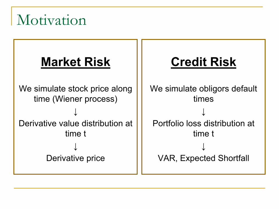
Motivation
Market Risk
We simulate stock price along time (Wiener process)
↓Derivative value distribution at
time t↓
Derivative price
Credit Risk
We simulate obligors default times
↓Portfolio loss distribution at
time t↓
VAR, Expected Shortfall
Motivation
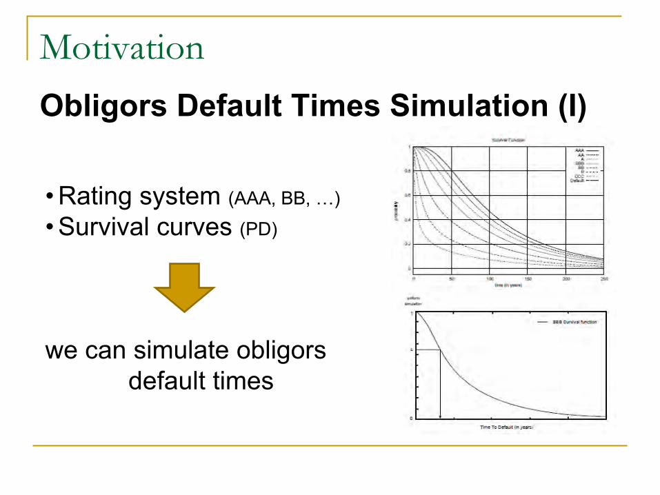
• Rating system (AAA, BB, …)
• Survival curves (PD)
we can simulate obligorsdefault times
Obligors Default Times Simulation (I)
Motivation
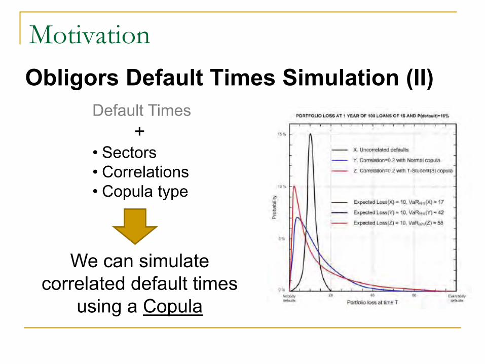
Default Times+
• Sectors• Correlations• Copula type
Obligors Default Times Simulation (II)
We can simulate correlated default times
using a Copula
Motivation
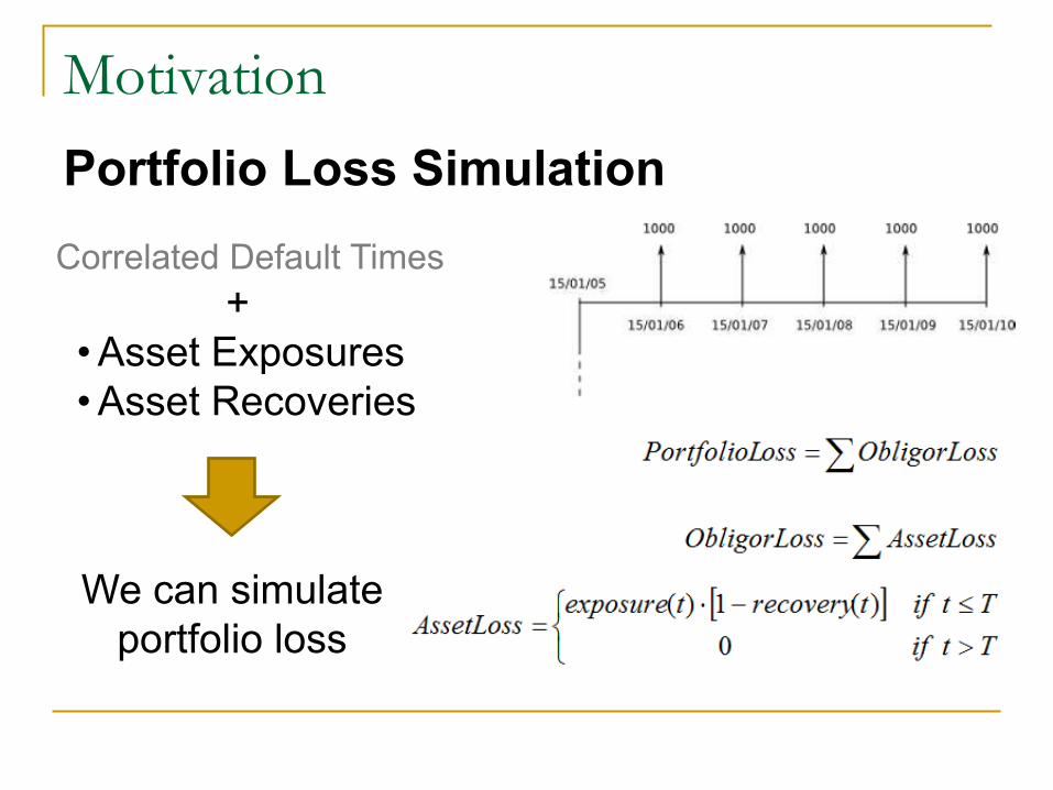
Portfolio Loss SimulationCorrelated Default Times
+• Asset Exposures• Asset Recoveries
We can simulate portfolio loss
Motivation
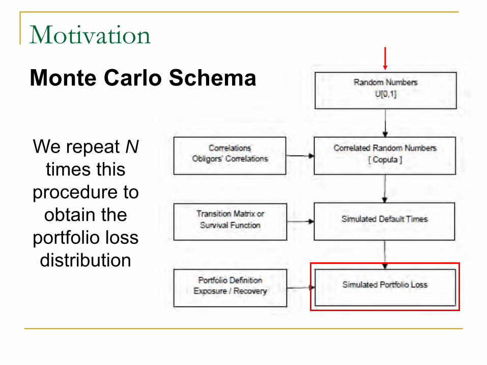
Monte Carlo Schema
We repeat Ntimes this
procedure to obtain the
portfolio loss distribution
Motivation
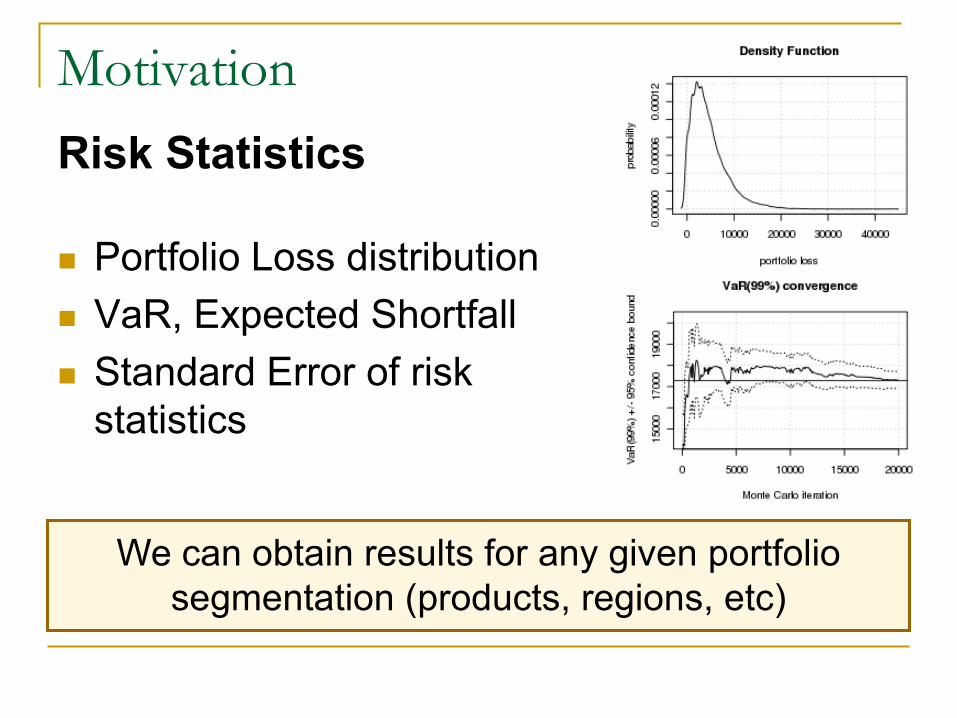
Portfolio Loss distribution VaR, Expected Shortfall Standard Error of risk
statistics
We can obtain results for any given portfolio segmentation (products, regions, etc)
Risk Statistics
Motivation
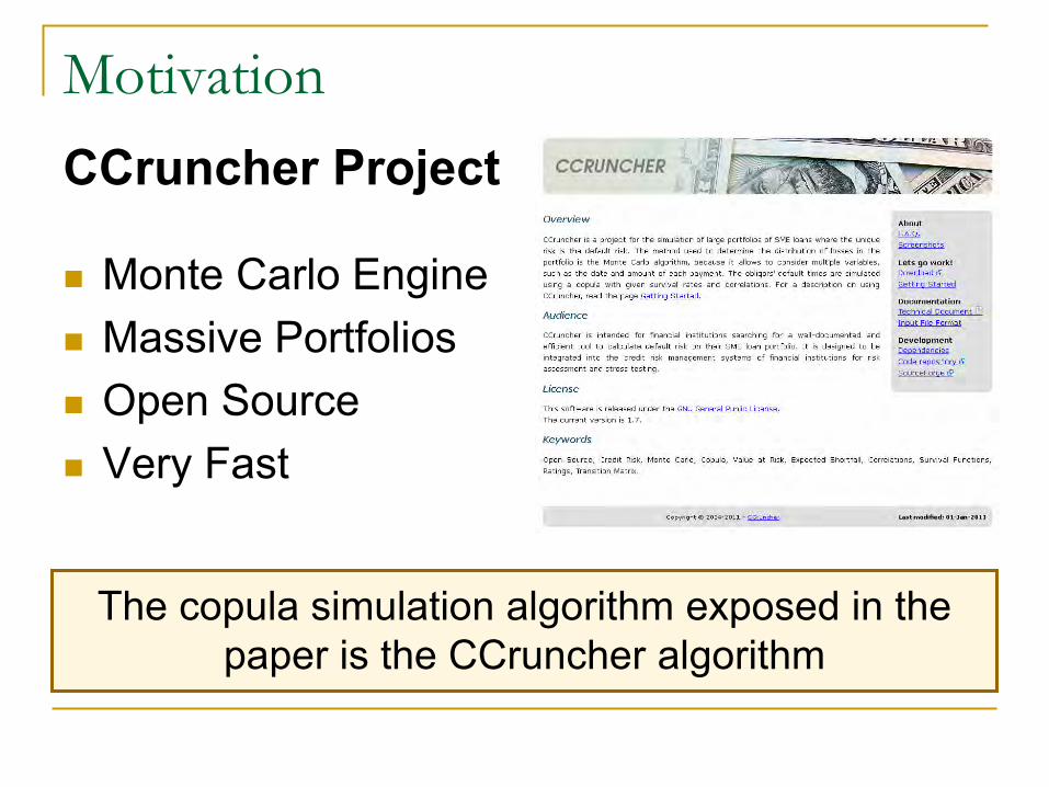
Monte Carlo Engine Massive Portfolios Open Source Very Fast
CCruncher Project
The copula simulation algorithm exposed in the paper is the CCruncher algorithm
Index
Motivation
The t-Student Copula
Block Matrices
Spearman’s Rank
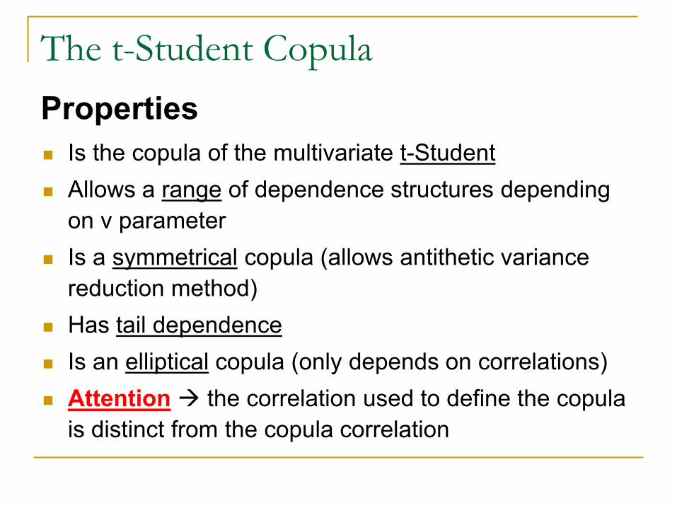
The t-Student Copula
Is the copula of the multivariate t-Student Allows a range of dependence structures depending
on v parameter Is a symmetrical copula (allows antithetic variance
reduction method) Has tail dependence Is an elliptical copula (only depends on correlations) Attention the correlation used to define the copula
is distinct from the copula correlation
Properties
The t-Student Copula
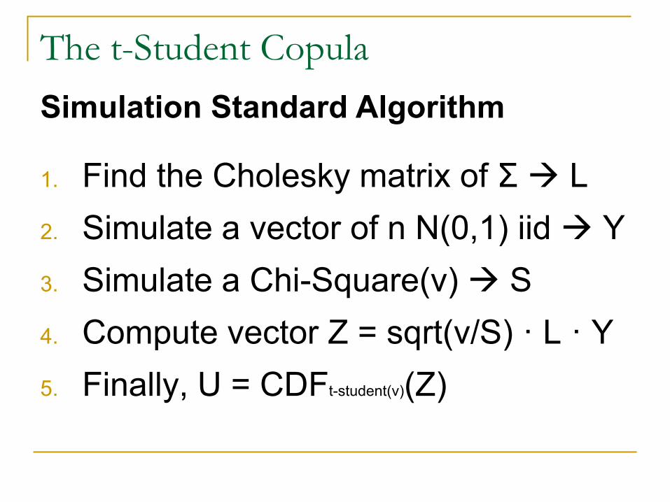
1. Find the Cholesky matrix of Σ L2. Simulate a vector of n N(0,1) iid Y3. Simulate a Chi-Square(v) S4. Compute vector Z = sqrt(v/S) · L · Y5. Finally, U = CDFt-student(v)(Z)
Simulation Standard Algorithm

Index
Motivation
The t-Student Copula
Block Matrices
Spearman’s Rank
Block Matrices
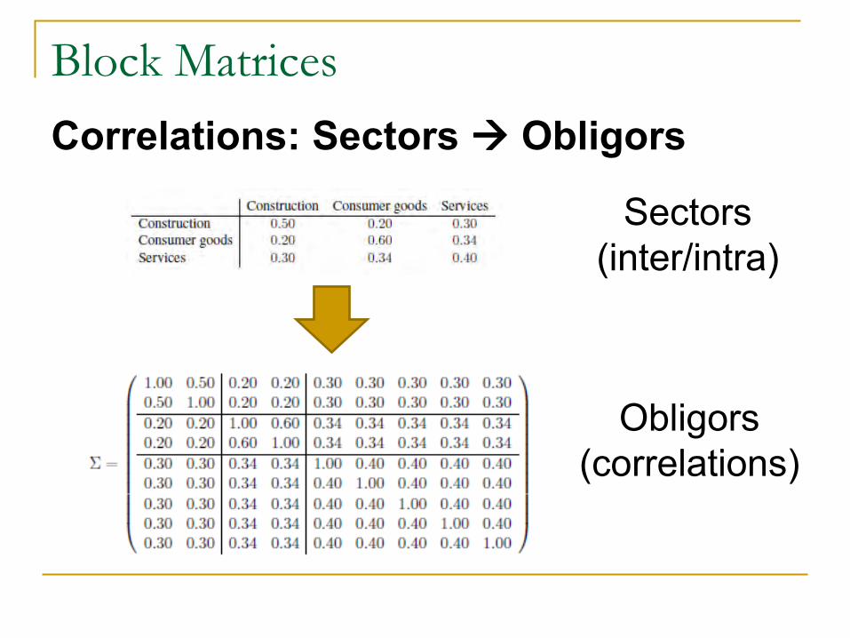
Correlations: Sectors Obligors
Sectors(inter/intra)
Obligors(correlations)
Block Matrices
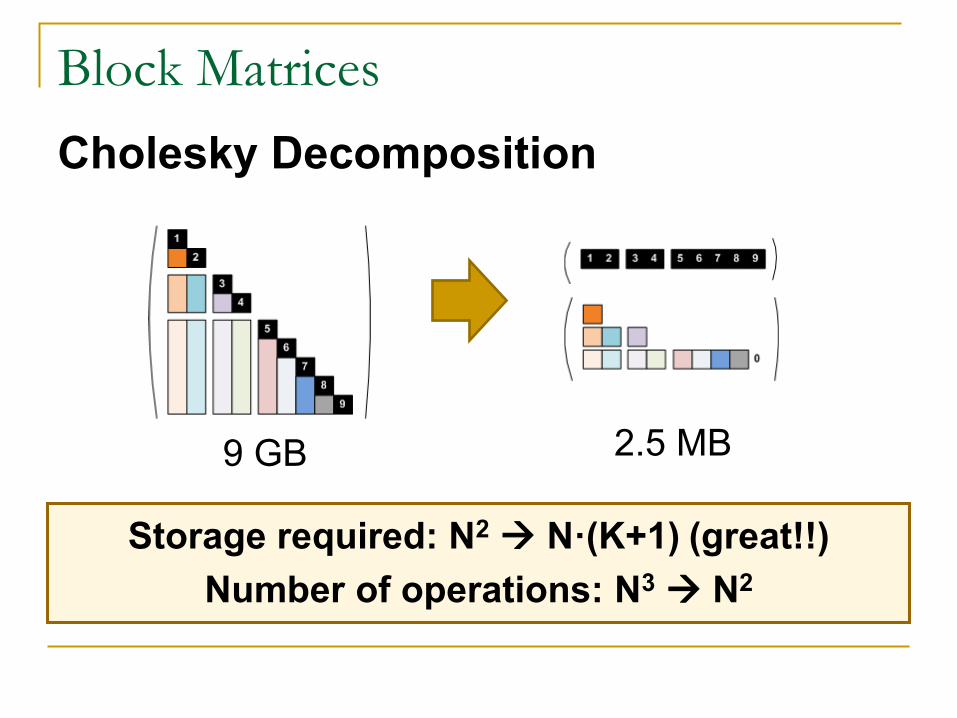
Storage required: N2 N·(K+1) (great!!)
Number of operations: N3 N2
Cholesky Decomposition
9 GB 2.5 MB
Block Matrices
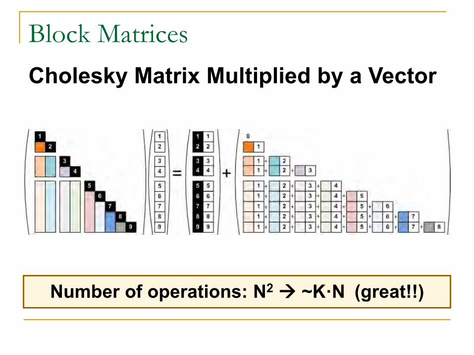
Number of operations: N2 ~K·N (great!!)
Cholesky Matrix Multiplied by a Vector
Block Matrices
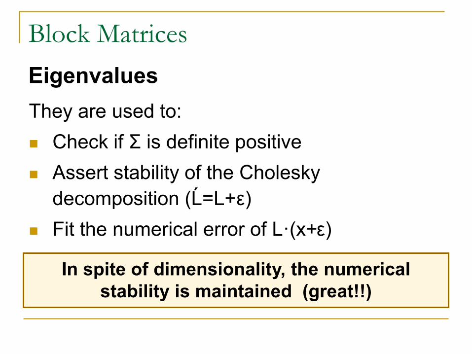
They are used to: Check if Σ is definite positive Assert stability of the Cholesky
decomposition (Ĺ=L+ε) Fit the numerical error of L·(x+ε)
Eigenvalues
In spite of dimensionality, the numerical stability is maintained (great!!)
Index
Motivation
The t-Student Copula
Block Matrices
Spearman’s Rank
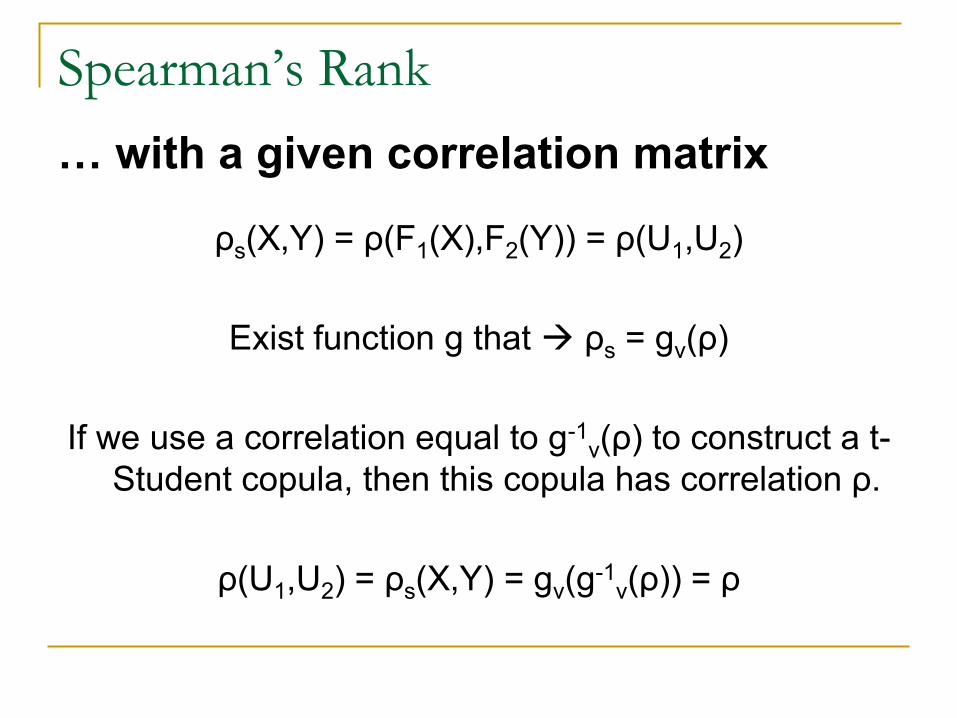
Spearman’s Rank
ρs(X,Y) = ρ(F1(X),F2(Y)) = ρ(U1,U2)
Exist function g that ρs = gν(ρ)
If we use a correlation equal to g-1ν(ρ) to construct a t-
Student copula, then this copula has correlation ρ.
ρ(U1,U2) = ρs(X,Y) = gν(g-1ν(ρ)) = ρ
… with a given correlation matrix
Spearman’s Rank
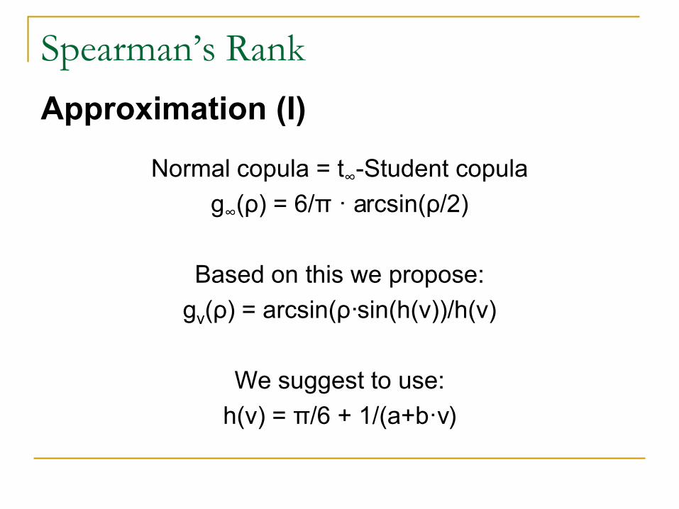
Normal copula = t∞-Student copulag∞(ρ) = 6/π · arcsin(ρ/2)
Based on this we propose:gv(ρ) = arcsin(ρ·sin(h(v))/h(v)
We suggest to use:h(v) = π/6 + 1/(a+b·v)
Approximation (I)
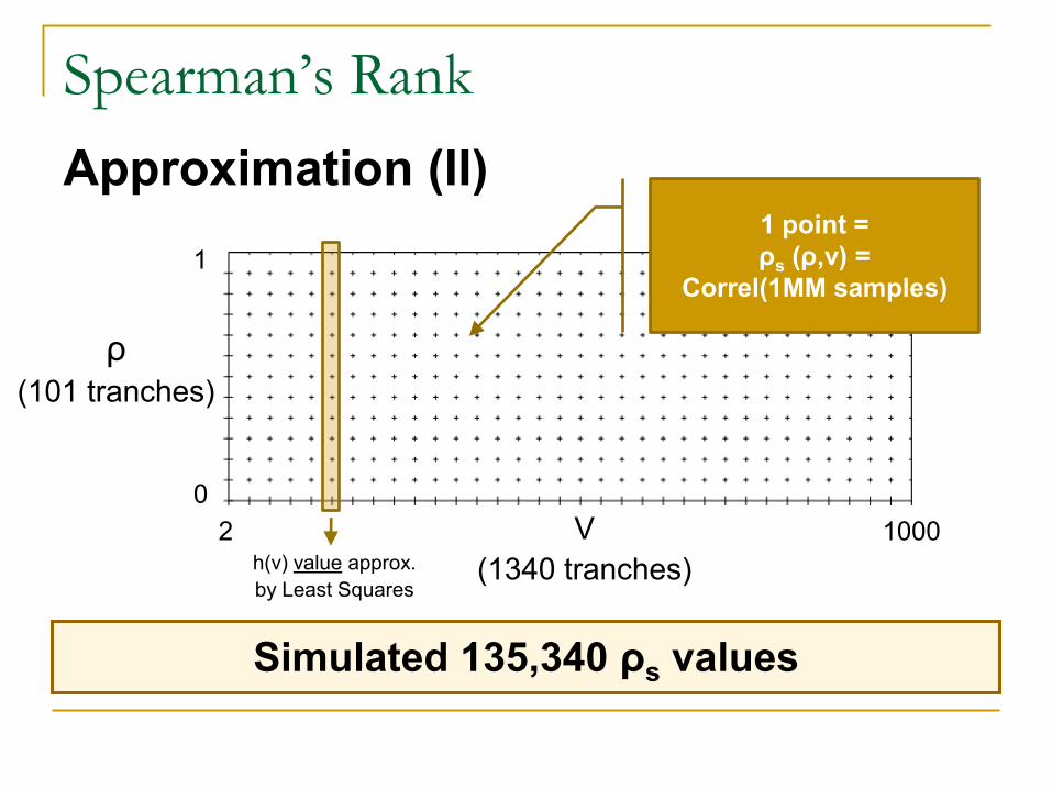
Spearman’s Rank
V(1340 tranches)
Approximation (II)
Simulated 135,340 ρs values
ρ(101 tranches)
1 point =ρs (ρ,v) =
Correl(1MM samples)
h(v) value approx.by Least Squares
1
02 1000
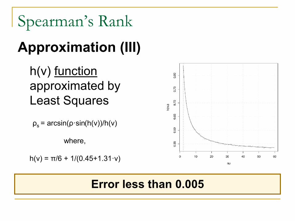
Spearman’s Rank
h(v) functionapproximated by Least Squares
Approximation (III)
Error less than 0.005
ρs = arcsin(ρ·sin(h(v))/h(v)
where,
h(v) = π/6 + 1/(0.45+1.31·v)

Summary
Portfolio Credit Risk Large Portfolios Monte Carlo Open Source CCruncher
Thank you !
Contact us: Gerard Torrent ([email protected]) Josep Fortiana ([email protected])
Useful links: http://www.ccruncher.net http://www.ccruncher.com


