137
Int. Jour. of Business & Inf. Tech. Vol-1 No. 1 June 2011
Solution of Stochastic Inventory Models with
Chance-Constraints by Intuitionistic Fuzzy
Optimization Technique S. Banerjee, T.K. Roy
Department of Mathematics, Bengal Engineering and Science University,
Shibpur, Howrah-711103, West Bengal, India
Abstract: Paknejad et al.’s model is analyzed in this paper
where the lead time demand follows normal distribution
under deterministic, stochastic and mixed environment,
respectively and thus the model becomes more realistic.
Expected annual cost is measured, with varying defective
rate. After that the Item wise multi objective models with
chance-constraints for both exponential and uniform lead
time demand are taken and the results are compared
numerically both in fuzzy optimization and intuitionistic
fuzzy optimization techniques. Objective of this paper is to
establish that intuitionistic fuzzy optimizaion method is
better than usual fuzzy optimization technique as expected
annual cost of this inventory model is more minimized in
case of intuitionistic fuzzy optimization method. Necessary
graphical presentations are also given besides numerical
illustrations.
Key-Words: Fuzzy optimizations, intuitionistic fuzzy
optimization, lead time demand, chance-constraint, multi-
objective stochastic model.
.
1. Introduction
Today most of the real-world decision-making
problems in economic, technical and environmental
ones are multi-dimensional and multi-objective. It is
significant to realize that multiple-objectives are often
non-commensurable and conflict with each other in
optimization problem. An objective within exact target
value is termed as fuzzy goal. So a multi-objective
model with fuzzy objectives is more realistic than
deterministic of it.
In conventional inventory models, uncertainties are
treated as randomness and are handled by appealing to
probability theory. However, in certain situations
uncertainties are due to fuzziness and these cases the
fuzzy set theory, originally introduced by Zadeh [23] is
applicable. In decision making process, first, Bellman
and Zadeh[6] introduced fuzzy set theory, Tanaka et. al.
[42] applied concept of fuzzy sets to decision making
problems to consider the objectives as fuzzy goals over
the α-cuts of a fuzzy constraints. Zimmerman [44, 45]
showed the classical algorithms can be used in few
inventory models. Li, Kabadi and Nair [28] discussed
fuzzy models for single-period inventory problem in
2002. Abou-El-Ata, Fergany and Wakeel[1] considered
in 2003, a probabilistic multi-item inventory model
With varying order cost. A single-period inventory
model with fuzzy demand isanalyzed by Kao and Hsu
[7]. Fergany, H.A. and El-Wakeel[8] considered a
probabilistic single-item inventory problem with
varying order cost under two linear constraints. A
survey of literature on continuously deteriorating
inventory models is discussed by F. Raafat[10]. Hala
and EI-Saadani[11] analyzed a constrained single
period stochastic uniform inventory model with
continuous distributions of demand and varying holding
cost. some inventory problems with fuzzy shortage cost
is discussed by Hideki Katagiri and Hiroaki [13]. I.
Moon and S. Choi[14] implemented A note on lead
time and distributional assumptions in continuous
review inventory models. Lai and Hwang [24,25]
elaborately discussed fuzzy mathematical programming
and fuzzy multiple objective decision making in their
two renowned contributions. Liang-Yuh and Hung-Chi
[26] analyzed A minimax distribution free procedure
for mixed inventory models invoving variable lead time
with fuzzy lost sales. Mahapatra and Roy [29]
discussed fuzzy multi-objective mathematical
programming on reliability optimization model. Hariga
and Ben-Daya [32] considered some stochastic
inventory models with deterministic variable lead time.
A fuzzy EOQ model with demand-dependent unit cost
under limited storage capacity is implemented by Roy
and Maiti [41]. Zheng [43] discussed optimal control
policy for stochastic inventory systems with Markovian
discount opportunities. Jaggi and Arneja [15]
considered stochastic integrated vendor-buyer model
with unstable lead-time and set up cost. Sadi-Nezhad ,
Nahavandi and Nazemi [40] analyzed periodic and
continuous inventory models in the presence of fuzzy
costs. Halim , Giri and Choudhuri [12] discussed fuzzy
production planning models for an unreliable
production system with fuzzy production rate and
stochastic and fuzzy demand. Banerjee and Roy [2]
presented a probabilistic inventory model with fuzzy
cost components and fuzzy random variable.
Intuitionistic Fuzzy Set (IFS) was introduced by K.
Atanassov [17] and seems to be applicable to real world
problems. The concept of IFS can be viewed as an
alternative approach to define a fuzzy set in case where
available information is not sufficient for the definition
of an imprecise concept by means of a conventional
fuzzy set. Thus it is expected that, IFS can be used to
simulate human decision-making process and any
138
Int. Jour. of Business & Inf. Tech. Vol-1 No. 1 June 2011
activitities requiring human expertise and knowledge
that are inevitably imprecise or totally reliable. Here the
degree of rejection and satisfaction are considered so
that the sum of both values is always less than unity
[17]. Atanossov also analyzed Intuitionistic fuzzy sets
in a more explicit way. Atanassov[18] discussed an
Open problems in intuitionistic fuzzy sets theory. An
Interval valued intuitionistic fuzzy sets was analyzed by
Atanassov and Gargov[18]. Atanassov and
Kreinovich[19] implemented Intuitionistic fuzzy
interpretation of interval data. The temporal
intuitionistic fuzzy sets are discussed also by
Atanossov[20]. Intuitionistic fuzzy soft sets are
considered by Maji Biswas and Roy[31]. Nikolova,
Nikolov, Cornelis and Deschrijver[33] presented a
Survey of the research on intuitionistic fuzzy sets.
Rough intuitionistic fuzzy sets are analyzed by Rizvi,
Naqvi and Nadeem[39]. Angelov [35] implemented the
Optimization in an intuitionistic fuzzy environment. He
[36, 37] also contributed in his another two important
papers, based on Intuitionistic fuzzy optimization.
Pramanik and Roy [38] solved a vector optimization
problem using an Intuitionistic Fuzzy goal
programming. A transportation model is solved by Jana
and Roy [16] using multi-objective intuitionistic fuzzy
linear programming. Fidanova and Atanassov [9]
discussed generalized net models and intuitionistic
fuzzy estimation of the process of ant colony
optimization. Banerjee and Roy [3] analyzed a
probabilistic fixed order interval system by general
fuzzy programming technique and intuitionistic fuzzy
optimization technique. Banerjee and Roy [4] also
solved a stochastic inventory model with fuzzy cost
components by fuzzy geometric and intuitionistic fuzzy
geometric programming technique. Mahapatra and
Mahapatra [30] presented the redundancy optimization
by intuitionistic fuzzy multi-objective programming.
Banerjee and Roy [5] discussed the solution of a
constrained stochastic model by fuzzy geometric and
intuitionistic fuzzy geometric programming.
Paknejad et.al. [34] presented a quality adjusted
lot-sizing model with stochastic demand and constant
lead time and studied the benefits of lower setup cost in
the model. We note that the previous literature focuses
on the issue of setup cost reduction in which
information about lead-time demand, whether constant
or stochastic, is assumed completely known. . Liang-
Yuh and Hung-Chi[27] modifies Paknejad et al.‟s
inventory model by relaxing the assumption that the
stochastic demand during lead time follows a specific
probability distribution and by considering that the
unsatisfied demands are partially backordered. Also,
instead of having a stockout cost in the objective
function, a service level constraint is employed.
As a single objective stochastic inventory problem,
Paknejad et al.‟s model[34] is analyzed in this paper
under deterministic, stochastic and mixed environment,
respectively, where the lead time demand follows
normal distribution. Expected annual cost is measured,
with varying defective rate, in deterministic
environment. After that an Item wise multi objective
models with chance-constraints for both exponential
and uniform lead time demand are taken and the results
are compared numerically both in fuzzy optimization
and intuitionistic fuzzy optimization techniques.
Objective of this paper is to establish that intuitionistic
fuzzy optimizaion method is better than usual fuzzy
optimization technique as expected annual cost of this
inventory model is more minimized in case of
intuitionistic fuzzy optimization method. Necessary
graphical presentations are also given besides numerical
illustrations.
2. Mathematical Model
Paknejad et.al. [26] presented a quality adjusted
lot-sizing model with stochastic demand and constant
lead time and studied the benefits of lower setup cost in
the model. We note that the previous literature focuses
on the issue of setup cost reduction in which
information about lead-time demand, whether constant
or stochastic, is assumed completely known. This paper
considers Paknejad et al.‟s model along with the
notations and some assumptions that will be taken into
account throughout the paper. Each lot contains a
random number of defectives following binomial
distribution. After the arrival purchaser examines the
entire lot. An order of size Q is placed as soon as the
inventory position reaches the reorder point s. the
shortages are allowed and completely backordered.
Lead-time is constant and probability distribution of
lead-time demand is known.
Now, we use the following notations:
D = expected demand per year
Q = lot size
s = reorder point
K = setup cost
θ = defective rate in a lot of size Q, 0 ≤ θ ≤ 1
h = nondefective holding cost per unit per year
h = defective holding cost per unit per year
π = shortage cost per unit short
= cost of inspecting a single item in each lot
μ = expected demand during lead time
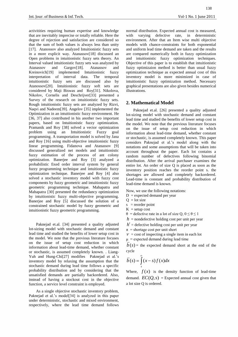
)(sb = the expected demand short at the end of the
cycle
s
dxxfsxsb )()()(
Where, )(xf is the density function of lead-time
demand. ),( sQEC = Expected annual cost given that
a lot size Q is ordered.
139
Int. Jour. of Business & Inf. Tech. Vol-1 No. 1 June 2011
3. Single Objective Stochastic Inventory
Model SOSIM)
Thus a quality adjusted lot-sizing model is formed
as:
),( sQMinEC = Setup cost + non-defective item
holding cost + stockout cost + defective item holding
cost + inspecting cost
=
1)1(
)1(
)(
)))1((2
1(
)1(
DvQh
Q
sbD
QshQ
DK
(3.1)
0, sQ
It is the stochastic model, which minimizes the
expected annual cost.
4. Multi Item Stochastic Inventory Model
(MISIM)
This model is analyzed here firstly in deterministic
environment and after that it is discussed in stochastic
and mixed environment also.
4.1 Model with deterministic budget and storage
To solve the problem in equation (3.1) as a MISIM,
it can be reformulated as:
),......,,,......,( 11 nn ssQQMinEC =
n
i 1
i
ii
iii
ii
iii
iiiiii
ii
ii
vDQh
Q
sbD
QshQ
KD
1)1(
)1(
)(
)))1((2
1(
)1(
Subject to
n
i
ii
n
i
ii
BQp
FQf
1
1
.,.......,2,10, nisQ ii
Here, For the i-th item (i =1, 2, ………….,n),
pi = price per unit item ,
fi = floor space available per unit,
n = number of item,
F = available floor space,
B = total budget.
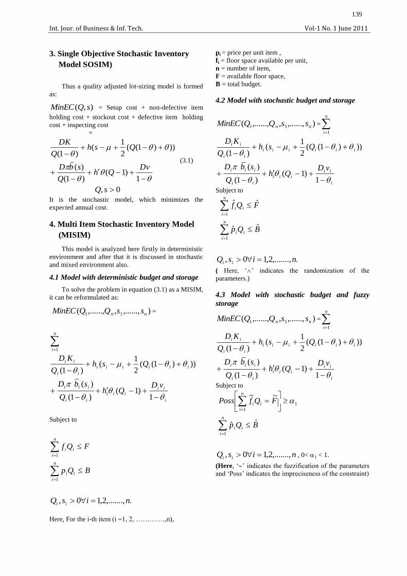
4.2 Model with stochastic budget and storage
),......,,,......,( 11 nn ssQQMinEC =
n
i 1
i
ii
iii
ii
iii
iiiiii
ii
ii
vDQh
Q
sbD
QshQ
KD
1)1(
)1(
)(
)))1((2
1(
)1(
Subject to
n
i
ii
n
i
ii
BQp
FQf
1
1
ˆˆ
ˆˆ
.,.......,2,10, nisQ ii
( Here, „‟ indicates the randomization of the
parameters.)
4.3 Model with stochastic budget and fuzzy
storage
),......,,,......,( 11 nn ssQQMinEC =
n
i 1
i
ii
iii
ii
iii
iiiiii
ii
ii
vDQh
Q
sbD
QshQ
KD
1)1(
)1(
)(
)))1((2
1(
)1(
Subject to
n
i
ii
n
i
ii
BQp
FQfPoss
1
1
1
ˆˆ
~~
nisQ ii ,.......,2,10, , 0< 1 < 1.
(Here, „‟ indicates the fuzzification of the parameters
and „Poss‟ indicates the impreciseness of the constraint)

140
Int. Jour. of Business & Inf. Tech. Vol-1 No. 1 June 2011
5 .Multi-Objective Stochastic Inventory
Model (MOSIM)
In reality, a managerial problem of a responsible
organization involves several conflicting objectives to
be achieved simultaneously subject to a system of
restrictions (constraints) that refers to a situation on
which the DM has no control. For this purpose a latest
tool is linear or non-linear programming problem with
multiple conflicting objectives. So the following model
which is an item wise multi objective may be
considered:
),( iii sQMinEC
i
ii
iii
ii
iii
iiiiii
ii
ii
vDQh
Q
sbD
QshQ
KD
1)1(
)1(
)(
)))1((2
1(
)1(
.,.......,2,10, nisQ ii
5.1 Model with deterministic budget and storage
),( iii sQMinEC
i
ii
iii
ii
iii
iiiiii
ii
ii
vDQh
Q
sbD
QshQ
KD
1)1(
)1(
)(
)))1((2
1(
)1(
Subject to
n
i
ii
n
i
ii
BQp
FQf
1
1
.,.......,2,10, nisQ ii
5.2 Model with stochastic budget and storage
),( iii sQMinEC
i
ii
iii
ii
iii
iiiiii
ii
ii
vDQh
Q
sbD
QshQ
KD
1)1(
)1(
)(
)))1((2
1(
)1(
Subject to
n
i
ii
n
i
ii
BQp
FQf
1
1
ˆˆ
ˆˆ
.,.......,2,10, nisQ ii
( Here, „‟ indicates the randomization of the
parameters.)
5.3 Model with stochastic budget and fuzzy
storage
),( iii sQMinEC
i
ii
iii
ii
iii
iiiiii
ii
ii
vDQh
Q
sbD
QshQ
KD
1)1(
)1(
)(
)))1((2
1(
)1(
Subject to
n
i
ii
n
i
ii
BQp
FQfPoss
1
1
1
ˆˆ
~~
.,.......,2,10, nisQ ii
( Here, „‟ indicates the fuzzification of the
parameters and „Poss‟ indicates the impreciseness of
the constraint)
6. Fuzzy Non-linear Programming (FNLP)
Technique to Solve Multi-Objective

141
Int. Jour. of Business & Inf. Tech. Vol-1 No. 1 June 2011
Non-Linear Programming Problem
(MONLP)
A Multi-Objective Non-Linear Programming
(MONLP) or Vector Minimization problem (VMP)
may be taken in the following form:
T
k xfxfxfxM ))(,),........(),(()inf( 21
Subject to
},......,2,1)(:{ mforjbororxgRxXx jj
n
….(6.1)
and ),....,2,1( niuxl ii
Zimmermann [36] showed that fuzzy programming
technique can be used to solve the multi-objective
programming problem.
To solve MONLP problem, following steps are used:
STEP 1: Solve the MONLP of equation (6.1) as a
single objective non-linear programming problem using
only one objective at a time and ignoring the others,
these solutions are known as ideal solution.
STEP 2: From the result of step1, determine the
corresponding values for every objective at each
solution derived. With the values of all objectives at
each ideal solution, pay-off matrix can be formulated as
follows:
)(........)()( 21 xfxfxf k
kx
x
x
....
2
1
)(....)()(
................
)(....)()(
)(....)()(
*
21
22*
2
2
1
11
2
1*
1
k
k
kk
k
k
xfxfxf
xfxfxf
xfxfxf
Here kxxx ,......,, 21
are the ideal solutions of the
objective functions )(),.......,(),( 21 xfxfxf k
respectively.
So
)}(),.......(),(max{ 21 krrrr xfxfxfU
and
)}(),.......(),(min{ 21 krrrr xfxfxfL
[Lr and Ur be lower and upper bounds of the thr
objective functions )(xf r ),.....,2,1 kr ]
STEP 3: Using aspiration level of each objective of the
MONLP of equation (6.1) may be written as follows:
Find x so as to satisfy
rr Lxf ~
)( ),........,2,1( kr
Xx
Here objective functions of equation (6.1) are
considered as fuzzy constraints. These type of fuzzy
constraints can be quantified by eliciting a
corresponding membership function:
0)(( xf rr or 0 if rr Uxf )(
)(( xf rr if rrr UxfL )(
),........,2,1( kr
= 1 if rr Lxf )(
….(6.2)
Having elicited the membership functions (as in
equation (6.2)) )(( xf rr for r = 1, 2, …… , k,
introduce a general aggregation function
))).((....,)),.......(()),((()( 2211~ xfxfxfGx kkD
So a fuzzy multi-objective decision making problem
can be defined as
Max )(~ xD
subject to Xx
….(6.3)
Here we adopt the fuzzy decision as:
Fuzzy decision based on minimum operator (like
Zimmermann‟s approach [44]. In this case equation
(6.3) is known as FNLPM.
Then the problem of equation (6.3), using the
membership function as in equation (6.2), according to
min-operator is reduced to:
Max
….(6.4)
Subject to )(( xf ii for
),........,2,1 ki
Xx ]1,0[
STEP 4: Solve the equation (6.4) to get optimal
solution.
7. Mathematical Analysis
A stochastic non-linear programming problem is
considered as:
Min f0(X)
Subject to
fj(X) cj (j=1, 2, ………..,m)
X 0.
142
Int. Jour. of Business & Inf. Tech. Vol-1 No. 1 June 2011
i.e Min f0(X)
….(7.1.1)
Subject to
fj(X) 0 (j=1, 2, ………..,m)
X 0.
Where, fj(X) = fj(X) - cj
Here X is a vector of N random variables y1, y2,
……….,yn and it includes the decision variables x1, x2,
……….,xn.
Expanding the objective function f0(X) about the mean
value iy of iy and neglecting the higher order term:
ii
N
i i
yyXy
fXfXf
1
0
00 )()( = )(X
(say) ….(7.1.2)
If yi (i=1, 2, ……. ,n) follow normal distribution then
so does )(X . The mean and variance of )(X are
given by:
= )(X
….(7.1.3)
2
2
1
0
iy
N
i i
Xy
f
….(7.1.4)
When some of the parameters of the constraints are
random in nature then the constraints will be
probabilistic and thus, the constraints can be written as:
jj rfP )0( (j=1,2 , ………,m)
….(7.1.5)
Then in the light of the theoretical convention
given above, equivalent deterministic constraints are:
0)(
2/1
2
1
iy
N
i i
j
jjj Xy
frf (j=1,2 ,
………,m) ….(7.1.6)
where, )( jj r is the value of the standard normal
variate corresponding to the probability rj.
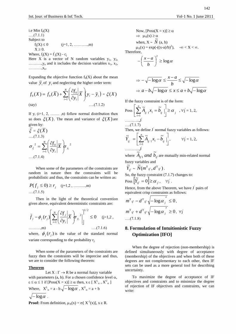
When some of the parameters of the constraints are
fuzzy then the constraints will be imprecise and thus,
we are to consider the following theorem:
Theorem
Let X : R be a normal fuzzy variable
with parameters (a, b). For a chosen confidence level ,
1 if [Poss(X = x)] then, x [ XL , X
U ]
Where, XL = a - b log , X
U = a + b
log .
Proof: From definition, X(x) = [ X-1
(x)], x R.
Now, [Poss(X = x)]
X(x)
when, X N~
(a, b)
X(x) = exp(-((x-a)/b)2), - < X < .
Therefore,
log
2
b
ax
loglog
b
ax
loglog baxba
If the fuzzy constraint is of the form:
Poss j
n
iijij
bxA
1
11
~~ , j
= 1, 2,
………..,J
….(7.1.7)
Then, we define J normal fuzzy variables as follows:
ij
Y~
n
iijij
bxA1
11
~~, j
= 1, 2,
………..,J
where 1
~jiA and jib
~are mutually min-related normal
fuzzy variables and
jiY
~ ),(
~ji
Yji
Y dmN .
So, the fuzzy constraint (7.1.7) changes to:
Poss jjiY 0~
, j .
Hence, from the above Theorem, we have J pairs of
equivalent crisp constraints as follows:
0log
jjiY
jiY dm ,
0log
jjiY
jiY dm , j
….(7.1.8)
8. Formulation of Intuitionistic Fuzzy
Optimization [IFO]
When the degree of rejection (non-membership) is
defined simultaneously with degree of acceptance
(membership) of the objectives and when both of these
degrees are not complementary to each other, then IF
sets can be used as a more general tool for describing
uncertainty.
To maximize the degree of acceptance of IF
objectives and constraints and to minimize the degree
of rejection of IF objectives and constraints, we can
write:
143
Int. Jour. of Business & Inf. Tech. Vol-1 No. 1 June 2011
nK,1,2,......i ,),(min
nK,1,2,......i ,),( max
i
i
RXX
RXX
Subject to
0
1)()(
)()(
,0)(
X
XX
XX
X
ii
ii
i
Where )(Xi denotes the degree of membership
function of )(X to the thi IF sets and )(Xi denotes
the degree of non-membership (rejection) of )(X from
the thi IF sets.
9. An Intuitionistic Fuzzy Approach for
Solving MOIP with Linear Membership
and Non-Membership Functions
To define the membership function of MOIM
problem, let acc
kL and acc
kU be the lower and upper
bounds of the thk objective function. These values are
determined as follows: Calculate the individual
minimum value of each objective function as a single
objective IP subject to the given set of constraints. Let **
2
*
1 ,......, kXXX be the respective optimal solution
for the k different objective and evaluate each objective
function at all these k optimal solution. It is assumed
here that at least two of these solutions are different for
which the thk objective function has different bounded
values. For each objective, find lower bound (minimum
value) acc
kL and the upper bound (maximum value)
acc
kU . But in intuitionistic fuzzy optimization (IFO),
the degree of rejection (non-membership) and degree of
acceptance (membership) are considered so that the
sum of both values is less than one. To define
membership function of MOIM problem, letrej
kL and
rej
kU be the lower and upper bound of the objective
function )(XZ k where acc
kL rej
kL rej
kU acc
kU . These values are defined as follows:
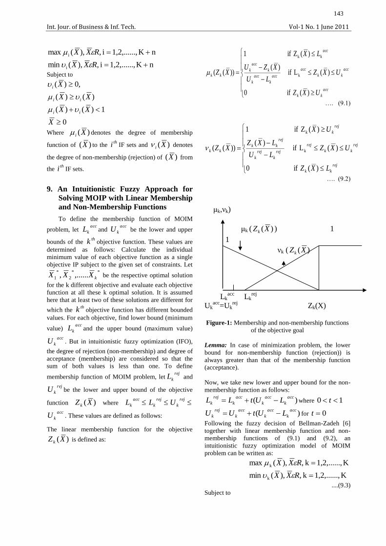
The linear membership function for the objective
)(XZ k is defined as:
)( if 0
)(L if )(
)( Zif 1
))(( k
k
acc
kk
acc
kk
acc
acc
k
acc
k
k
acc
k
acc
k
kk
UXZ
UXZLU
XZU
LX
XZ
…. (9.1)
)( if 0
)(L if )(
)( Zif 1
))(( k
k
rej
kk
rej
kk
rej
rej
k
rej
k
rej
kk
rej
k
kk
LXZ
UXZLU
LXZ
UX
XZ
…. (9.2)
μk,νk)
μk ( )(XZk ) 1
1
νk ( )(XZk
Lkacc
Lkrej
Ukacc
=Ukrej
Zk(X)
Figure-1: Membership and non-membership functions
of the objective goal
Lemma: In case of minimization problem, the lower
bound for non-membership function (rejection)) is
always greater than that of the membership function
(acceptance).
Now, we take new lower and upper bound for the non-
membership function as follows:
)(acc
k
acc
k
acc
k
rej
k LUtLL where 10 t
)(acc
k
acc
k
acc
k
rej
k LUtUU for 0t
Following the fuzzy decision of Bellman-Zadeh [6]
together with linear membership function and non-
membership functions of (9.1) and (9.2), an
intuitionistic fuzzy optimization model of MOIM
problem can be written as:
K,1,2,......k ,),(min
K,1,2,......k ,),( max
k
k
RXX
RXX
....(9.3)
Subject to
144
Int. Jour. of Business & Inf. Tech. Vol-1 No. 1 June 2011
0
1)()(
)()(
,0)(
X
XX
XX
X
kk
kk
k
The problem of equation (9.3) can be reduced following
Angelov [35] to the following form:
Max
….(9.4)
Subject to
)()(acc
k
acc
k
acc
kk LUUXZ
)()(rej
k
rej
k
rej
kk LULXZ
0
1
0
X
Then the solution of the MOIM problem is summarized
in the following steps:
Step 1. Pick the first objective function and solve it as a
single objective IP subject to the constraint, continue
the process K-times for K different objective functions.
If all the solutions (i.e.
n),1,2,......j ;,.....,2,1(......**
2
*
1 miXXX k
same, then one of them is the optimal compromise
solution and go to step 6. Otherwise go to step 2.
However, this rarely happens due to the conflicting
objective functions.
Then the intuitionistic fuzzy goals take the form
)(XZ k kk XL *)(~ .,.......,2,1 Kk ,
Step 2. To build membership function, goals and
tolerances should be determined at first. Using the ideal
solutions, obtained in step 1, we find the values of all
the objective functions at each ideal solution and
construct pay off matrix as follows:
)(............)()(
........................
........................
........................
)(............)()(
)(............)()(
**
2
*
1
*
2
*
22
*
21
*
1
*
12
*
11
kkkk
k
k
XZXZXZ
XZXZXZ
XZXZXZ
Step 3. From Step 2, we find the upper and lower
bounds of each objective for the degree of acceptance
and rejection corresponding to the set of solutions as
follows:
acc
kU = ))(max(*
rk XZ and acc
kL =
))(min(*
rk XZ
kr 1 kr 1
For linear membership functions,
)(acc
k
acc
k
acc
k
rej
k LUtLL where 10 t
)(acc
k
acc
k
acc
k
rej
k LUtUU for 0t
Step 4. Construct the fuzzy programming problem of
equation (9.3) and find its equivalent LP problem of
equation (9.4).
Step 5. Solve equation (9.4) by using appropriate
mathematical programming algorithm to get an optimal
solution and evaluate the K objective functions at these
optimal compromise solutions
.
Step 6. STOP.
10. Few Stochastic Models
CASE 1: Demand follows Uniform distribution
We assume that lead time demand for the
period for the thi item is a random variable which
follows uniform distribution and if the decision maker
feels that demand values for item I below ia or above
ib are highly unlikely and values between ia and ib
are equally likely, then the probability density function
)(xf i are given by:
)(xf i =
otherwise 0
a if 1
i i
ii
bxab
for
.,.....,2,1 ni
So, )(2
)()(
2
ii
ii
iiab
sbsb
for .,.....,2,1 ni
….(10.1)
Where, )( ii sb are the expected number of shortages
per cycle and all these values of )( ii sb affect all the
desired models.
CASE 2: Demand follows Exponential distribution
We assume that lead-time demand for the
period for the thi item is a random variable that follows
145
Int. Jour. of Business & Inf. Tech. Vol-1 No. 1 June 2011
exponential distribution. Then the probability density
function )(xf i are given by:
)(xf i = )( x
iie ,
x>0 for .,.....,2,1 ni
= 0, otherwise
So, )(
)(i
s
ii
iiesb
for .,.....,2,1 ni
….(10.2)
Where, )( ii sb are the expected number of shortages
per cycle and all these values of )( ii sb affect all the
desired models.
CASE 3: Demand follows Normal distribution
We assume that lead-time demand for the
period for the ith item is a random variable, which
follows normal distribution. Then the probability
density function fi(x) are given by:
)2/)(exp(2
1)(
22
ii
i
i xxf
,
x
)2/)(exp(2
1
))(1(2
)()(
22
iii
i
ii
i
ii
ii
s
sssb
for .,.....,2,1 ni ….(10.3)
Where, )( ii sb are the expected number of shortages
per cycle and all these values of )( ii sb affects all the
desired models and )( ix represents area under
standard normal curve from -∞ to ix .
11. Numericals
A. Solution of the model (3.1)
We consider the following data:
D=2750; K=10; h=0.25; v =0.02; π =1; h =0.15.
[All the cost related parameters are measured in „$‟]
Here, the lead time demand follows Normal distribution
with mean (μ) =20 and standard deviation (σ) =2.
The expected demand short at the end of the cycle takes
up the value as:
)2/)(exp(2
1
))(1(2
)()(
22
s
sssb
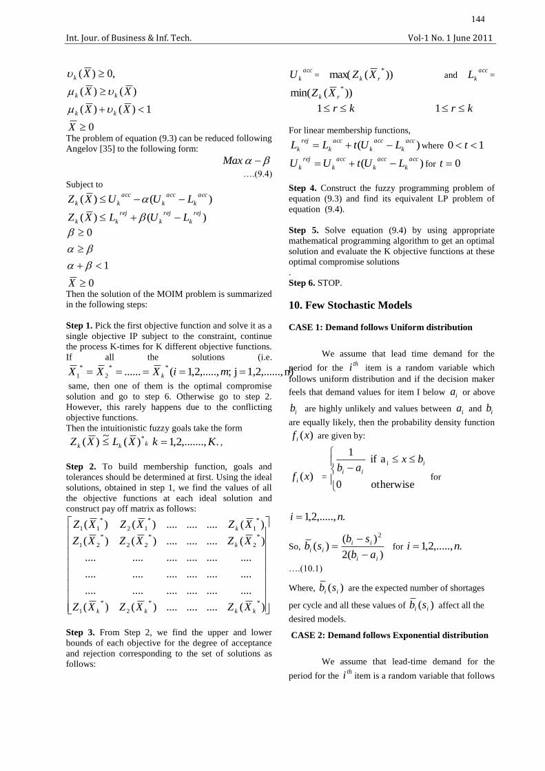
In the Table-1, a study of expected annual cost EC (Q,
s) with lot size Q and reorder point s is given for
different defective rate θ. We conclude from the
following Table-1 as well as graph-1 that, the order
quantity as well as the expected annual cost increase as
θ increases.
θ EC* (Q, s) Q
*
0.1 186.3471 489.2484
0.2 202.8538 513.7929
0.3 223.2740 543.9329
0.4 249.3887 581.9080
0.5 284.3121 631.4677
0.6 334.0731 699.4850
0.7 412.2208 800.3515
0.8 557.5926 971.4324
0.9 952.6872 1361.609
Graph-1: B. Solution of the model (4.1), (4.2) and
(4.3). In this case our objective is to analyze the
expected annual cost of the Multi-item model in
deterministic, stochastic and mixed environment
respectively when the lead-time demand follows normal
distribution and thus the model becomes more practical
and realistic.
0
200
400
600
800
1000
1200
1400
θ 0.1 0.2 0.3 0.4 0.5 0.6 0.7 0.8 0.9
EC* (Q, s) 186.347 202.854 223.274 249.389 284.312 334.073 412.221 557.593 952.687
Q* 489.248 513.793 543.933 581.908 631.468 699.485 800.352 971.432 1361.61
1 2 3 4 5 6 7 8 9
146
Int. Jour. of Business & Inf. Tech. Vol-1 No. 1 June 2011
To solve (4.1), we use the methods described in the
section 7 and the following data are considered:
D1=2750; K1=10; h1=0.25; θ1=0.3; μ1= 20; σ1= 2;
v1=0.02; π1=2; 1h =0.15; p1=2.
D2=2700; K2=14; h2 =0.65; θ2=0.5; μ2 = 10; σ2= 1;
v2=0.01; π2=1; 2h =0.35; p2=4.
B=40000, F=50000, f1=2, f2=3.
For model (4.2) the following data are taken:
D1=2750; K1=10; h1=0.25; θ1=0.3; μ1= 20; σ1= 2;
v1=0.02; π1=2; 1h =0.15; D2=2700; K2=14; h2 =0.65;
θ2=0.5; μ2 = 10; σ2= 1; v2=0.01; π2=1; 2h =0.35; 1p̂
=(3, 0.03), 1f̂ =(2,0.02), r=0.95, 2p̂ =(2, 0.02) 2f̂ =(3,
0.03) B̂ =(40000, 40) F̂ =(50000,50).
For model (4.3) the following data are taken:
D1=2750; K1=10; h1=0.25; θ1=0.3; μ1= 20; σ1= 2;
v1=0.02; π1=2; 1h =0.15; D2=2700; K2=14; h2 =0.65;
θ2=0.5; μ2 = 10; σ2= 1; v2=0.01; π2=1; 2h =0.35; 1p̂
=(1, 0.01), 1
~f =(1,0.01), r=0.95, 2p̂ =(2, 0.02) 2
~f =(3,
0.03) B̂ =(50000, 60) F~
=(60000,60), 1=0.5.
[All the cost related parameters are measured in „$‟]
Thus, we have the results obtained below:
Table-2
Models
under
Normal
Distribution
EC($) Q1 Q2 s1 s2
Determinist
ic
Environmen
t
1331.2
1
473.2
6
297.1
2
41.2
2
61.3
2
Stochastic
Environmen
t
1294.7
6
488.1
4
797.0
6 4.34 6.58
Mixed
Environmen
t
912.19 388.4
0
297.8
4
18.4
2
11.6
5
C. Solution of the model (5.1), (5.2), (5.3)
In case of intuitionistic fuzzy optimization not only the
membership function is maximized but also, the non-
membership function is minimized (as it is described
in section 8 and 9), whereas in the fuzzy optimization
technique only the memberships function is
maximized (as in section 6). So, our objective is to
establish the fact that IFO makes the betterment of
the solution than FO.
To solve MOSIM of section 5.1, we use the methods
described in the sections 6, 7, 8 and 9 and the following
data are considered:
Case1. The lead time demand follows uniform
distribution and thus )( ii sb , the expected demand
short at the end of the cycle takes up the value
according to (10.1).
We consider two different set of data as:
D1=2700; K1=12; h1=0.55; θ1=0.6; μ1=(a1+b1)/2; v1
=0.03; π1=1; h 1=0.25; a1=20; b1=70; μ1=(a1+b1)/2,
p1=3, f1=2.
D2=2750; K2=10; h2=0.25; θ2=0.8; μ2=(a2+b2)/2; v2
=0.02; π2=2; h 2=0.15; a2=10; b2=50; μ2=(a2+b2)/2,
p2=2, f2=3, B=40000, F=50000.
[All the cost related parameters are measured in „$‟]
The pay-off matrix is:
EC1 EC2
5142.5743421.852
5697.7992213.512
We take, U1acc
=852.3421; L1acc
=512.2213;
U2acc
=799.5697; L2acc
=574.5142;
U1rej
=852.3421; L1rej
=530; U2rej
=799.5697;
L2rej
=598.
Table-3: Comparison of solutions of FO and IFO in
deterministic environment
(UNIFORM LEAD-TIME DEMAND)
MET
HODS
Q1 Q2 s1 S2 EC1
($)
EC2
($)
α*
β*
Fuzzy
Optim
izatio
n
42
3.
7
10
66.
6
71.
78
4
49.
45
3
522.
348
7
591.
768
3
0.
7
9
--
Intuiti
onistic
Fuzzy
optimi
zation
97
0.
5
11
54.
4
64.
43
2
51.
65
4
518.
321
9
567.
650
8
0.
8
9
0.
04
5
147
Int. Jour. of Business & Inf. Tech. Vol-1 No. 1 June 2011
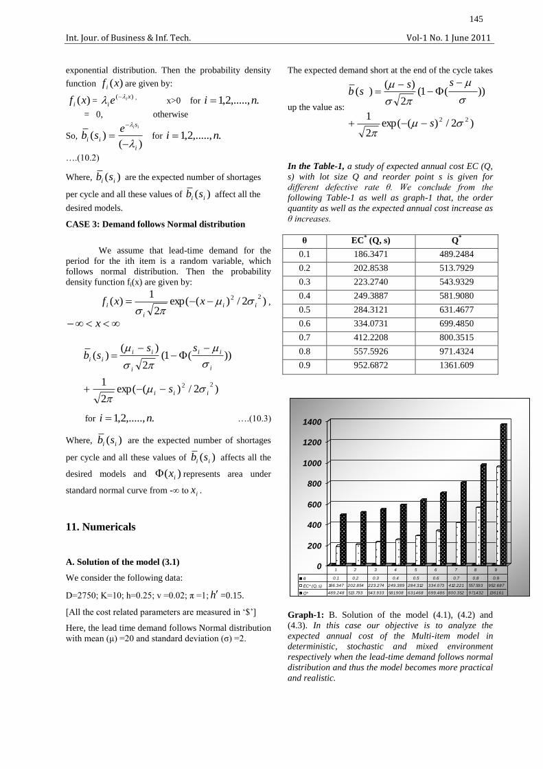
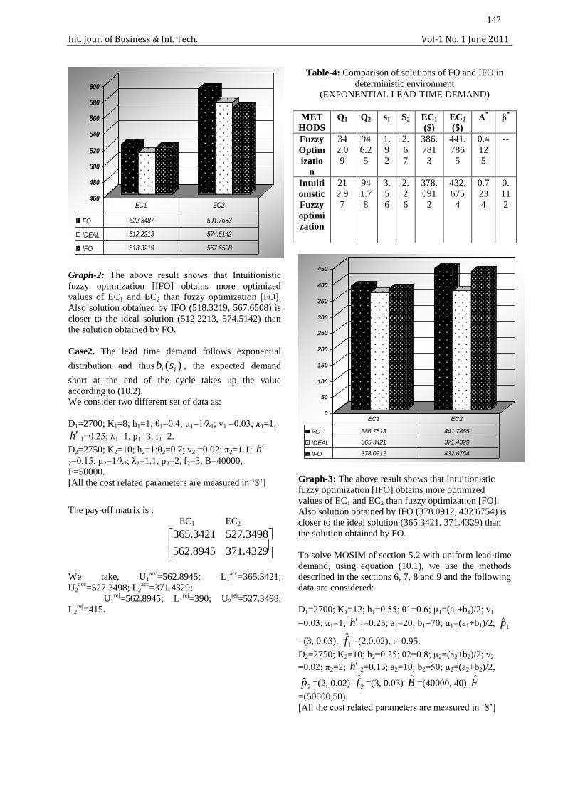
Graph-2: The above result shows that Intuitionistic
fuzzy optimization [IFO] obtains more optimized
values of EC1 and EC2 than fuzzy optimization [FO].
Also solution obtained by IFO (518.3219, 567.6508) is
closer to the ideal solution (512.2213, 574.5142) than
the solution obtained by FO.
Case2. The lead time demand follows exponential
distribution and thus )( ii sb , the expected demand
short at the end of the cycle takes up the value
according to (10.2).
We consider two different set of data as:
D1=2700; K1=8; h1=1; θ1=0.4; μ1=1/λ1; v1 =0.03; π1=1;
h 1=0.25; λ1=1, p1=3, f1=2.
D2=2750; K2=10; h2=1;θ2=0.7; v2 =0.02; π2=1.1; h
2=0.15; μ2=1/λ2; λ2=1.1, p2=2, f2=3, B=40000,
F=50000.
[All the cost related parameters are measured in „$‟]
The pay-off matrix is :
EC1 EC2
4329.3718945.562
3498.5273421.365
We take, U1acc
=562.8945; L1acc
=365.3421;
U2acc
=527.3498; L2acc
=371.4329;
U1rej
=562.8945; L1rej
=390; U2rej
=527.3498;
L2rej
=415.
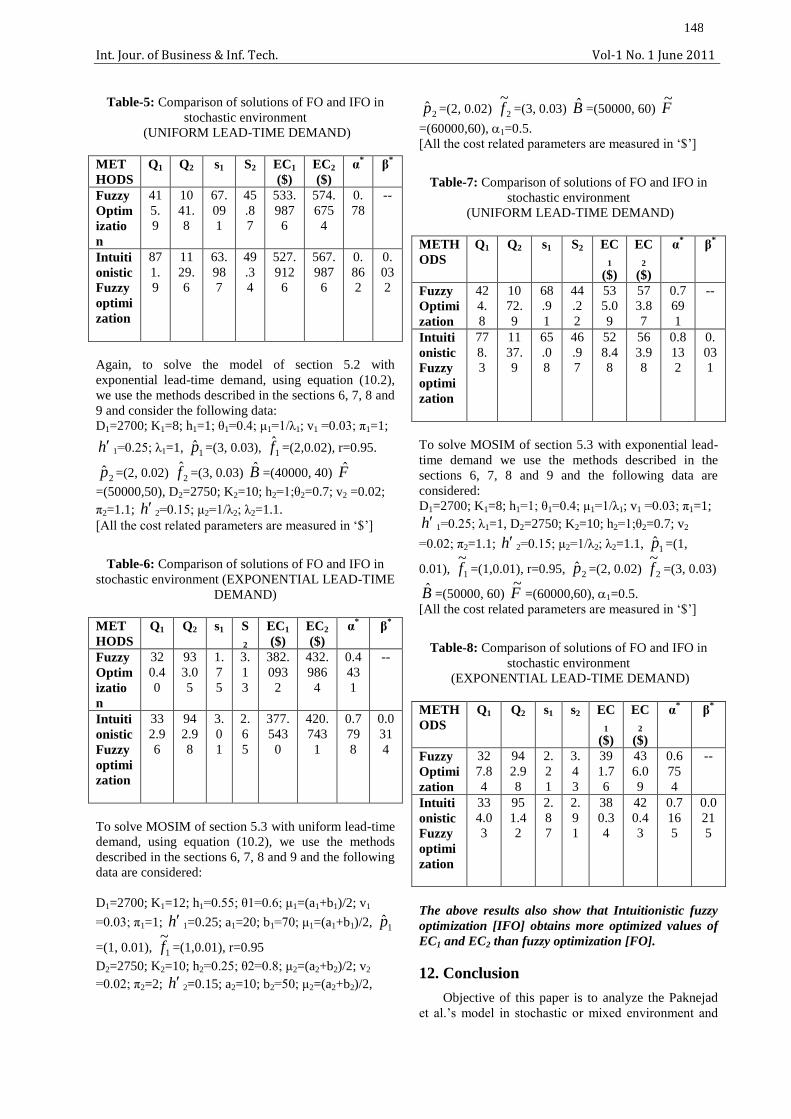
Table-4: Comparison of solutions of FO and IFO in
deterministic environment
(EXPONENTIAL LEAD-TIME DEMAND)
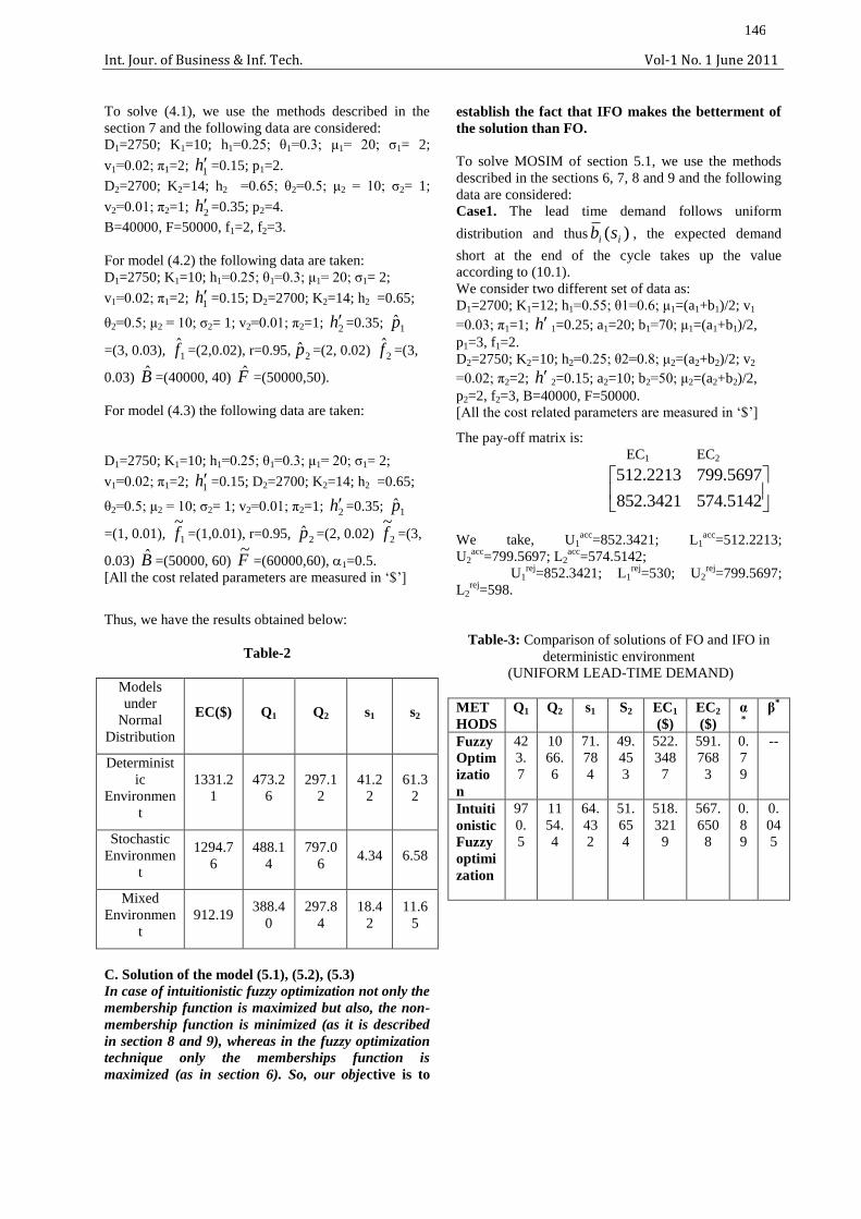
Graph-3: The above result shows that Intuitionistic
fuzzy optimization [IFO] obtains more optimized
values of EC1 and EC2 than fuzzy optimization [FO].
Also solution obtained by IFO (378.0912, 432.6754) is
closer to the ideal solution (365.3421, 371.4329) than
the solution obtained by FO.
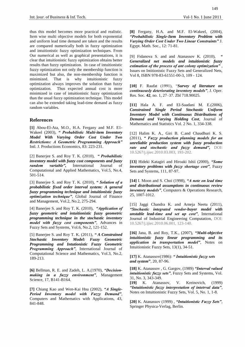
To solve MOSIM of section 5.2 with uniform lead-time
demand, using equation (10.1), we use the methods
described in the sections 6, 7, 8 and 9 and the following
data are considered:
D1=2700; K1=12; h1=0.55; θ1=0.6; μ1=(a1+b1)/2; v1
=0.03; π1=1; h 1=0.25; a1=20; b1=70; μ1=(a1+b1)/2, 1p̂
=(3, 0.03), 1f̂ =(2,0.02), r=0.95.
D2=2750; K2=10; h2=0.25; θ2=0.8; μ2=(a2+b2)/2; v2
=0.02; π2=2; h 2=0.15; a2=10; b2=50; μ2=(a2+b2)/2,
2p̂ =(2, 0.02) 2f̂ =(3, 0.03) B̂ =(40000, 40) F̂
=(50000,50).
[All the cost related parameters are measured in „$‟]
460
480
500
520
540
560
580
600
FO 522.3487 591.7683
IDEAL 512.2213 574.5142
IFO 518.3219 567.6508
EC1 EC2
0
50
100
150
200
250
300
350
400
450
FO 386.7813 441.7865
IDEAL 365.3421 371.4329
IFO 378.0912 432.6754
EC1 EC2
MET
HODS
Q1 Q2 s1 S2 EC1
($)
EC2
($)
Α*
β*
Fuzzy
Optim
izatio
n
34
2.0
9
94
6.2
5
1.
9
2
2.
6
7
386.
781
3
441.
786
5
0.4
12
5
--
Intuiti
onistic
Fuzzy
optimi
zation
21
2.9
7
94
1.7
8
3.
5
6
2.
2
6
378.
091
2
432.
675
4
0.7
23
4
0.
11
2
148
Int. Jour. of Business & Inf. Tech. Vol-1 No. 1 June 2011
Table-5: Comparison of solutions of FO and IFO in
stochastic environment
(UNIFORM LEAD-TIME DEMAND)
MET
HODS
Q1 Q2 s1 S2 EC1
($)
EC2
($)
α*
β*
Fuzzy
Optim
izatio
n
41
5.
9
10
41.
8
67.
09
1
45
.8
7
533.
987
6
574.
675
4
0.
78
--
Intuiti
onistic
Fuzzy
optimi
zation
87
1.
9
11
29.
6
63.
98
7
49
.3
4
527.
912
6
567.
987
6
0.
86
2
0.
03
2
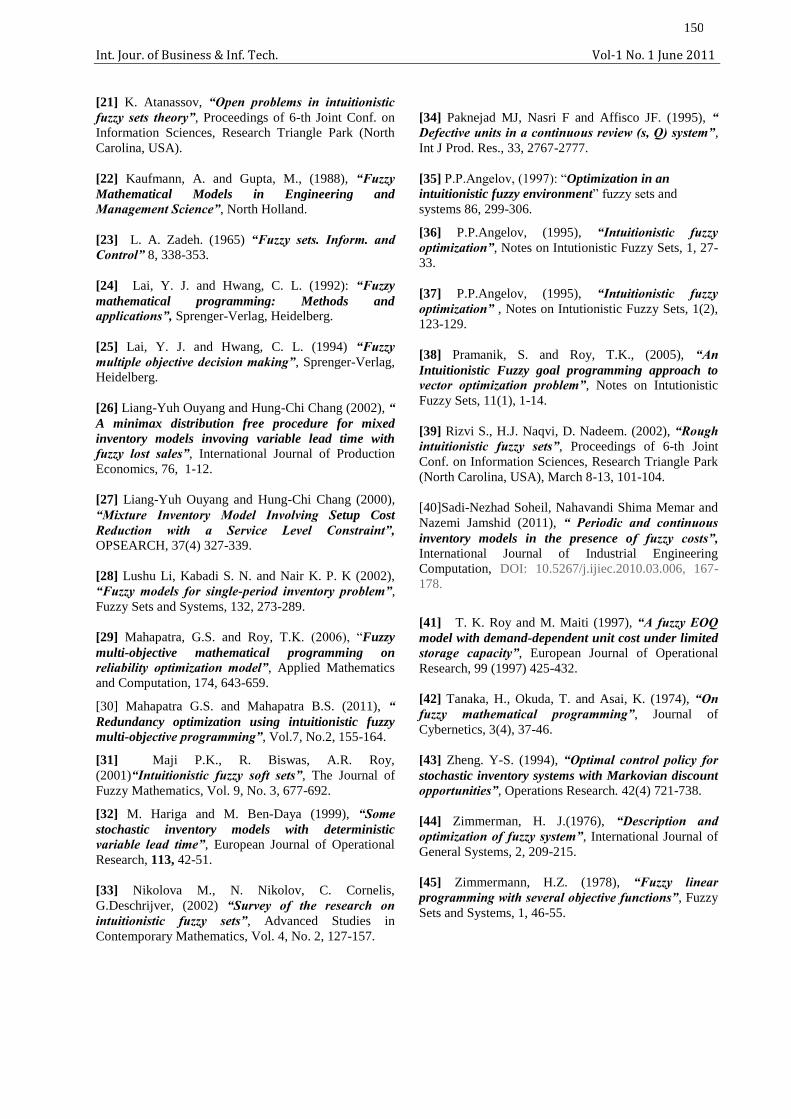
Again, to solve the model of section 5.2 with
exponential lead-time demand, using equation (10.2),
we use the methods described in the sections 6, 7, 8 and
9 and consider the following data:
D1=2700; K1=8; h1=1; θ1=0.4; μ1=1/λ1; v1 =0.03; π1=1;
h 1=0.25; λ1=1, 1p̂ =(3, 0.03), 1f̂ =(2,0.02), r=0.95.
2p̂ =(2, 0.02) 2f̂ =(3, 0.03) B̂ =(40000, 40) F̂
=(50000,50), D2=2750; K2=10; h2=1;θ2=0.7; v2 =0.02;
π2=1.1; h 2=0.15; μ2=1/λ2; λ2=1.1.
[All the cost related parameters are measured in „$‟]
Table-6: Comparison of solutions of FO and IFO in
stochastic environment (EXPONENTIAL LEAD-TIME
DEMAND)
MET
HODS
Q1 Q2 s1 S
2
EC1
($)
EC2
($)
α*
β*
Fuzzy
Optim
izatio
n
32
0.4
0
93
3.0
5
1.
7
5
3.
1
3
382.
093
2
432.
986
4
0.4
43
1
--
Intuiti
onistic
Fuzzy
optimi
zation
33
2.9
6
94
2.9
8
3.
0
1
2.
6
5
377.
543
0
420.
743
1
0.7
79
8
0.0
31
4
To solve MOSIM of section 5.3 with uniform lead-time
demand, using equation (10.2), we use the methods
described in the sections 6, 7, 8 and 9 and the following
data are considered:
D1=2700; K1=12; h1=0.55; θ1=0.6; μ1=(a1+b1)/2; v1
=0.03; π1=1; h 1=0.25; a1=20; b1=70; μ1=(a1+b1)/2, 1p̂
=(1, 0.01), 1
~f =(1,0.01), r=0.95
D2=2750; K2=10; h2=0.25; θ2=0.8; μ2=(a2+b2)/2; v2
=0.02; π2=2; h 2=0.15; a2=10; b2=50; μ2=(a2+b2)/2,
2p̂ =(2, 0.02) 2
~f =(3, 0.03) B̂ =(50000, 60) F
~
=(60000,60), 1=0.5.
[All the cost related parameters are measured in „$‟]
Table-7: Comparison of solutions of FO and IFO in
stochastic environment
(UNIFORM LEAD-TIME DEMAND)
METH
ODS
Q1 Q2 s1 S2 EC
1
($)
EC
2
($)
α*
β*
Fuzzy
Optimi
zation
42
4.
8
10
72.
9
68
.9
1
44
.2
2
53
5.0
9
57
3.8
7
0.7
69
1
--
Intuiti
onistic
Fuzzy
optimi
zation
77
8.
3
11
37.
9
65
.0
8
46
.9
7
52
8.4
8
56
3.9
8
0.8
13
2
0.
03
1
To solve MOSIM of section 5.3 with exponential lead-
time demand we use the methods described in the
sections 6, 7, 8 and 9 and the following data are
considered:
D1=2700; K1=8; h1=1; θ1=0.4; μ1=1/λ1; v1 =0.03; π1=1;
h 1=0.25; λ1=1, D2=2750; K2=10; h2=1;θ2=0.7; v2
=0.02; π2=1.1; h 2=0.15; μ2=1/λ2; λ2=1.1, 1p̂ =(1,
0.01), 1
~f =(1,0.01), r=0.95, 2p̂ =(2, 0.02) 2
~f =(3, 0.03)
B̂ =(50000, 60) F~
=(60000,60), 1=0.5.
[All the cost related parameters are measured in „$‟]
Table-8: Comparison of solutions of FO and IFO in
stochastic environment
(EXPONENTIAL LEAD-TIME DEMAND)
METH
ODS
Q1 Q2 s1 s2 EC
1
($)
EC
2
($)
α*
β*
Fuzzy
Optimi
zation
32
7.8
4
94
2.9
8
2.
2
1
3.
4
3
39
1.7
6
43
6.0
9
0.6
75
4
--
Intuiti
onistic
Fuzzy
optimi
zation
33
4.0
3
95
1.4
2
2.
8
7
2.
9
1
38
0.3
4
42
0.4
3
0.7
16
5
0.0
21
5
The above results also show that Intuitionistic fuzzy
optimization [IFO] obtains more optimized values of
EC1 and EC2 than fuzzy optimization [FO].
12. Conclusion
Objective of this paper is to analyze the Paknejad
et al.‟s model in stochastic or mixed environment and
149
Int. Jour. of Business & Inf. Tech. Vol-1 No. 1 June 2011
thus this model becomes more practical and realistic.
Item wise multi objective models for both exponential
and uniform lead time demand are taken and the results
are compared numerically both in fuzzy optimization
and intuitionistic fuzzy optimization techniques. From
Our numerical as well as graphical presentations, it is
clear that intuitionistic fuzzy optimization obtains better
results than fuzzy optimization. In case of intuitionistic
fuzzy optimization not only the membership function is
maximized but also, the non-membership function is
minimized. That is why intuitionistic fuzzy
optimization always improves the solution than fuzzy
optimization. Thus expected annual cost is more
minimized in case of intuitionistic fuzzy optimization
than the usual fuzzy optimization technique. This model
can also be extended taking lead-time demand as fuzzy
random variables.
References
[1] Abou-El-Ata, M.O., H.A. Fergany and M.F. E1-
Wakeel (2003), “ Probabilistic Multi-item Inventory
Model With Varying Order Cost Under Two
Restrictions: A Geometric Programming Approach”
Intl. J. Productions Economics, 83: 223-231.
[2] Banerjee S. and Roy T. K. (2010), “ Probabilistic
inventory model with fuzzy cost components and fuzzy
random variable”, International Journal of
Computational and Applied Mathematics, Vol.5, No.4,
501-514.
[3] Banerjee S. and Roy T. K. (2010), “ Solution of a
probabilistic fixed order interval system: A general
fuzzy programming technique and intuitionistic fuzzy
optimization technique”, Global Journal of Finance
and Management, Vol.2, No.2, 275-294.
[4] Banerjee S. and Roy T. K. (2010), “Application of
fuzzy geometric and intuitionistic fuzzy geometric
programming technique in the stochastic inventory
model with fuzzy cost components”, Advances in
Fuzzy Sets and Systems, Vol.6, No.2, 121-152.
[5] Banerjee S. and Roy T. K. (2011), “ A Constrained
Stochastic Inventory Model: Fuzzy Geometric
Programming and Intutionistic Fuzzy Geometric
Programming Approach”, International Journal of
Computational Science and Mathematics, Vol.3, No.2,
189-213.
[6] Bellman, R. E. and Zadeh, L. A.(1970), “Decision-
making in a fuzzy environment”, Management
Science, 17, B141-B164.
[7] Chiang Kao and Wen-Kai Hsu (2002), “A Single-
Period Inventory model with Fuzzy Demand”,
Computers and Mathematics with Applications, 43,
841-848.
[8] Fergany, H.A. and M.F. El-Wakeel, (2004),
“Probabilistic Single-Item Inventory Problem with
Varying Order Cost Under Two Linear Constraints” J.
Egypt. Math. Soc., 12: 71-81.
[9] Fidanova S. and and Atanassov K. (2010), “
Generalized net models and intuitionistic fuzzy
estimation of the process of ant colony optimization” ,
Issues on Intitionistic Fuzzy Sets and Generalized Nets, Vol 8, ISBN 978-83-61551-00-3, 109 - 124.
[10] F. Raafat (1991), “Survey of literature on
continuously deteriorating inventory models”, J. Oper.
Res. Soc. 42, no. 1, 27–37. Zbl 718.90025.
[11] Hala A. F. and EI-Saadani M. E.(2006),
Constrained Single Period Stochastic Uniform
Inventory Model with Continuous Distributions of
Demand and Varying Holding Cost, Journal of
Mathematics and Statistics Vol. 2 No. 1, 334-338.
[12] Halim K. A., Giri B. C.and Chaudhuri K. S.
(2011), “ Fuzzy production planning models for an
unreliable production system with fuzzy production
rate and stochastic and fuzzy demand”, DOI:
10.5267/j.ijiec.2010.03.003, 193-202.
[13] Hideki Katagiri and Hiroaki Ishii (2000), “Some
inventory problems with fuzzy shortage cost”, Fuzzy
Sets and Systems, 111, 87-97.
[14] I. Moon and S. Choi (1998), “A note on lead time
and distributional assumptions in continuous review
inventory models”, Computers & Operations Research,
25, 1007-1012.
[15] Jaggi Chandra K. and Arneja Neetu (2011),
“Stochastic integrated vendor-buyer model with
unstable lead-time and set up cost”, International
Journal of Industrial Engineering Computation, DOI:
10.5267/j.ijiec.2010.06.001, 123-140.
[16] Jana, B. and Roy, T.K., (2007), “Multi-objective
intuitionistic fuzzy linear programming and its
application in transportation model”, Notes on
Intuitionistic Fuzzy Sets, 13(1), 34-51.
[17] K. Atanassov(1986): “ Intuitionistic fuzzy sets
and system”, 20, 87-96.
[18] K. Atanassov , G. Gargov, (1989) “Interval valued
intuitionistic fuzzy sets”, Fuzzy Sets and Systems, Vol.
31, No. 3, 343-349.
[19] K. Atanassov, V. Kreinovich, (1999)
“Intuitionistic fuzzy interpretation of intetrval data”,
Notes on Intuitionistic Fuzzy Sets, Vol. 5, No. 1, 1-8.
[20] K. Atanassov (1999) , “Intuitionistic Fuzzy Sets”,
Springer Physica-Verlag, Berlin.
150
Int. Jour. of Business & Inf. Tech. Vol-1 No. 1 June 2011
[21] K. Atanassov, “Open problems in intuitionistic
fuzzy sets theory”, Proceedings of 6-th Joint Conf. on
Information Sciences, Research Triangle Park (North
Carolina, USA).
[22] Kaufmann, A. and Gupta, M., (1988), “Fuzzy
Mathematical Models in Engineering and
Management Science”, North Holland.
[23] L. A. Zadeh. (1965) “Fuzzy sets. Inform. and
Control” 8, 338-353.
[24] Lai, Y. J. and Hwang, C. L. (1992): “Fuzzy
mathematical programming: Methods and
applications”, Sprenger-Verlag, Heidelberg.
[25] Lai, Y. J. and Hwang, C. L. (1994) “Fuzzy
multiple objective decision making”, Sprenger-Verlag,
Heidelberg.
[26] Liang-Yuh Ouyang and Hung-Chi Chang (2002), “
A minimax distribution free procedure for mixed
inventory models invoving variable lead time with
fuzzy lost sales”, International Journal of Production
Economics, 76, 1-12.
[27] Liang-Yuh Ouyang and Hung-Chi Chang (2000),
“Mixture Inventory Model Involving Setup Cost
Reduction with a Service Level Constraint”, OPSEARCH, 37(4) 327-339.
[28] Lushu Li, Kabadi S. N. and Nair K. P. K (2002),
“Fuzzy models for single-period inventory problem”,
Fuzzy Sets and Systems, 132, 273-289.
[29] Mahapatra, G.S. and Roy, T.K. (2006), “Fuzzy
multi-objective mathematical programming on
reliability optimization model”, Applied Mathematics
and Computation, 174, 643-659.
[30] Mahapatra G.S. and Mahapatra B.S. (2011), “
Redundancy optimization using intuitionistic fuzzy
multi-objective programming”, Vol.7, No.2, 155-164.
[31] Maji P.K., R. Biswas, A.R. Roy,
(2001)“Intuitionistic fuzzy soft sets”, The Journal of
Fuzzy Mathematics, Vol. 9, No. 3, 677-692.
[32] M. Hariga and M. Ben-Daya (1999), “Some
stochastic inventory models with deterministic
variable lead time”, European Journal of Operational
Research, 113, 42-51.
[33] Nikolova M., N. Nikolov, C. Cornelis,
G.Deschrijver, (2002) “Survey of the research on
intuitionistic fuzzy sets”, Advanced Studies in
Contemporary Mathematics, Vol. 4, No. 2, 127-157.
[34] Paknejad MJ, Nasri F and Affisco JF. (1995), “
Defective units in a continuous review (s, Q) system”,
Int J Prod. Res., 33, 2767-2777.
[35] P.P.Angelov, (1997): “Optimization in an
intuitionistic fuzzy environment” fuzzy sets and
systems 86, 299-306.
[36] P.P.Angelov, (1995), “Intuitionistic fuzzy
optimization”, Notes on Intutionistic Fuzzy Sets, 1, 27-
33.
[37] P.P.Angelov, (1995), “Intuitionistic fuzzy
optimization” , Notes on Intutionistic Fuzzy Sets, 1(2),
123-129.
[38] Pramanik, S. and Roy, T.K., (2005), “An
Intuitionistic Fuzzy goal programming approach to
vector optimization problem”, Notes on Intutionistic
Fuzzy Sets, 11(1), 1-14.
[39] Rizvi S., H.J. Naqvi, D. Nadeem. (2002), “Rough
intuitionistic fuzzy sets”, Proceedings of 6-th Joint
Conf. on Information Sciences, Research Triangle Park
(North Carolina, USA), March 8-13, 101-104.
[40]Sadi-Nezhad Soheil, Nahavandi Shima Memar and
Nazemi Jamshid (2011), “ Periodic and continuous
inventory models in the presence of fuzzy costs”, International Journal of Industrial Engineering
Computation, DOI: 10.5267/j.ijiec.2010.03.006, 167-
178.
[41] T. K. Roy and M. Maiti (1997), “A fuzzy EOQ
model with demand-dependent unit cost under limited
storage capacity”, European Journal of Operational
Research, 99 (1997) 425-432.
[42] Tanaka, H., Okuda, T. and Asai, K. (1974), “On
fuzzy mathematical programming”, Journal of
Cybernetics, 3(4), 37-46.
[43] Zheng. Y-S. (1994), “Optimal control policy for
stochastic inventory systems with Markovian discount
opportunities”, Operations Research. 42(4) 721-738.
[44] Zimmerman, H. J.(1976), “Description and
optimization of fuzzy system”, International Journal of
General Systems, 2, 209-215.
[45] Zimmermann, H.Z. (1978), “Fuzzy linear
programming with several objective functions”, Fuzzy
Sets and Systems, 1, 46-55.


