Spatial Statistics Classification Spatial More
Spatial Statistics with Image Analysis
David Bolin1
1Mathematical StatisticsCentre for Mathematical Sciences
Lund University
Lund
October 5, 2012
David Bolin - [email protected] Spatial Statistics 1/35
Spatial Statistics Classification Spatial More
Outline
Spatial Statistics with Image Analysis
Hierarchical models
Estimation procedures
Pixel classification
K-means
Bayesian classification
EM-algorithm
Example
Spatial statistics
Image reconstruction
Ozone
Temperature
Learn more
David Bolin - [email protected] Spatial Statistics 2/35
Spatial Statistics Classification Spatial More Hierarchical Estimation
A statistical approach
◮ All measurements contain random measurement errors/variation.
◮ Most natural phenomena have natural random variation.
◮ Often the uncertainty of an estimate is, at least, as important as the
estimate it self.
◮ We need to describe and model random variation and uncertainties!
David Bolin - [email protected] Spatial Statistics 3/35
Spatial Statistics Classification Spatial More Hierarchical Estimation
Hierarchical models
◮ We often have some prior knowledge of the reality.
◮ Given knowledge of the true reality, what can we say about images
and other data?
◮ Construct a model for observations given that we know the truth.
◮ Given data, what can we say about the unknown reality?
This is the inverse problem.
David Bolin - [email protected] Spatial Statistics 4/35
Spatial Statistics Classification Spatial More Hierarchical Estimation
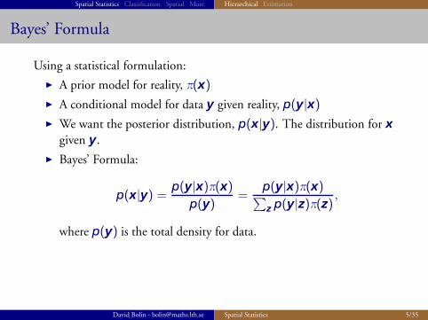
Bayes’ Formula
Using a statistical formulation:
◮ A prior model for reality, π(x)
◮ A conditional model for data y given reality, p(y|x)
◮ We want the posterior distribution, p(x|y). The distribution for x
given y.
◮ Bayes’ Formula:
p(x|y) =p(y|x)π(x)
p(y)=
p(y|x)π(x)∑z
p(y|z)π(z),
where p(y) is the total density for data.
David Bolin - [email protected] Spatial Statistics 5/35
Spatial Statistics Classification Spatial More Hierarchical Estimation
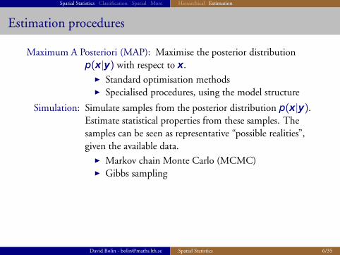
Estimation procedures
Maximum A Posteriori (MAP): Maximise the posterior distribution
p(x|y) with respect to x.
◮ Standard optimisation methods◮ Specialised procedures, using the model structure
Simulation: Simulate samples from the posterior distribution p(x|y).Estimate statistical properties from these samples. The
samples can be seen as representative “possible realities”,
given the available data.
◮ Markov chain Monte Carlo (MCMC)◮ Gibbs sampling
David Bolin - [email protected] Spatial Statistics 6/35
Spatial Statistics Classification Spatial More Hierarchical Estimation
Some examples
◮ Classification (K-means and the EM algorithm)◮ LANDSAT
◮ Dependence structures; Markov random fields◮ Image reconstruction◮ Reconstruction of fields — Global ozone and temperature
David Bolin - [email protected] Spatial Statistics 7/35
Spatial Statistics Classification Spatial More K-means Bayesian EM-algorithm Example
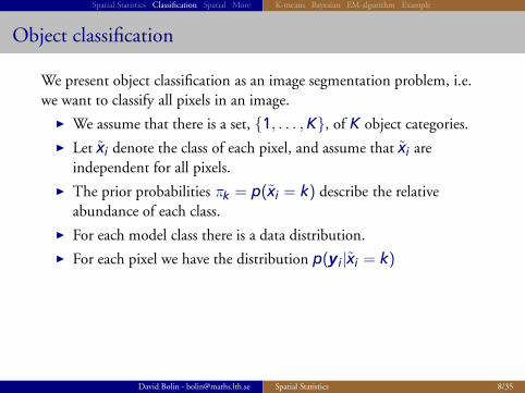
Object classification
We present object classification as an image segmentation problem, i.e.
we want to classify all pixels in an image.
◮ We assume that there is a set, {1, . . . ,K}, of K object categories.
◮ Let x̃i denote the class of each pixel, and assume that x̃i are
independent for all pixels.
◮ The prior probabilities πk = p(x̃i = k) describe the relative
abundance of each class.
◮ For each model class there is a data distribution.
◮ For each pixel we have the distribution p(yi|x̃i = k)
David Bolin - [email protected] Spatial Statistics 8/35
Spatial Statistics Classification Spatial More K-means Bayesian EM-algorithm Example
The K-means algorithm
The K-means algorithm is a simple, popular algorithm for separating
data into different clusters.
1. Select K data-points at random, as initial cluster centres.
2. Assign all data points to their nearest cluster centre.
3. Compute the mean within each cluster, and let these be the new
cluster centres.
4. Repeat from 2.
David Bolin - [email protected] Spatial Statistics 9/35
Spatial Statistics Classification Spatial More K-means Bayesian EM-algorithm Example
Drawbacks of K-means
◮ Handling of different πk?
◮ Different variation within clusters?
◮ Overlapping clusters?
If we assume that the data within each cluster is multivariate Normal,
how can we improve on K-means?
David Bolin - [email protected] Spatial Statistics 10/35
Spatial Statistics Classification Spatial More K-means Bayesian EM-algorithm Example
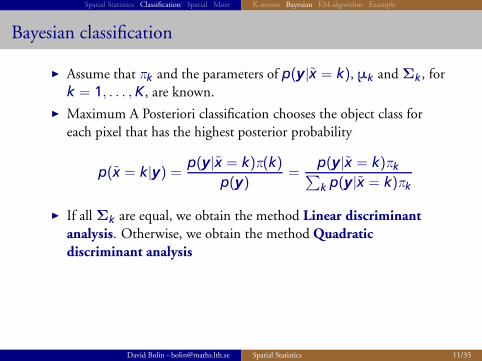
Bayesian classification
◮ Assume that πk and the parameters of p(y|x̃ = k), μk andΣk, for
k = 1, . . . ,K, are known.
◮ Maximum A Posteriori classification chooses the object class for
each pixel that has the highest posterior probability
p(x̃ = k|y) =p(y|x̃ = k)π(k)
p(y)=
p(y|x̃ = k)πk∑k p(y|x̃ = k)πk
◮ If allΣk are equal, we obtain the method Linear discriminant
analysis. Otherwise, we obtain the method Quadratic
discriminant analysis
David Bolin - [email protected] Spatial Statistics 11/35
Spatial Statistics Classification Spatial More K-means Bayesian EM-algorithm Example
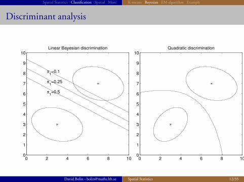
Discriminant analysis
0 2 4 6 8 100
1
2
3
4
5
6
7
8
9
10Linear Bayesian discrimination
π1=0.5
π1=0.25
π1=0.1
0 2 4 6 8 100
1
2
3
4
5
6
7
8
9
10Quadratic discrimination
David Bolin - [email protected] Spatial Statistics 12/35
Spatial Statistics Classification Spatial More K-means Bayesian EM-algorithm Example
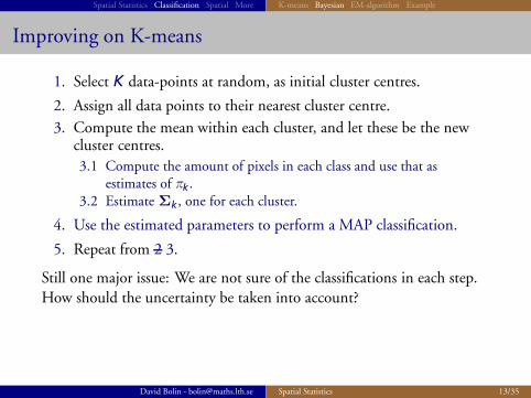
Improving on K-means
1. Select K data-points at random, as initial cluster centres.
2. Assign all data points to their nearest cluster centre.
3. Compute the mean within each cluster, and let these be the newcluster centres.
3.1 Compute the amount of pixels in each class and use that asestimates of πk.
3.2 EstimateΣk, one for each cluster.
4. Use the estimated parameters to perform a MAP classification.
5. Repeat from 2 3.
Still one major issue: We are not sure of the classifications in each step.
How should the uncertainty be taken into account?
David Bolin - [email protected] Spatial Statistics 13/35
Spatial Statistics Classification Spatial More K-means Bayesian EM-algorithm Example
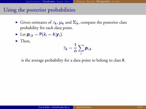
Using the posterior probabilities
◮ Given estimates of πk, μk andΣk, compute the posterior class
probability for each data point.
◮ Let pi,k = P(x̃i = k|yi).
◮ Then,
π̂k =1
n
∑
i
pi,k
is the average probability for a data point to belong to class k.
David Bolin - [email protected] Spatial Statistics 14/35
Spatial Statistics Classification Spatial More K-means Bayesian EM-algorithm Example
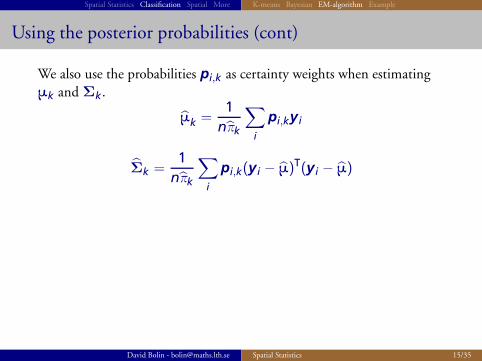
Using the posterior probabilities (cont)
We also use the probabilities pi,k as certainty weights when estimating
μk andΣk.
μ̂k =1
nπ̂k
∑
i
pi,kyi
Σ̂k =1
nπ̂k
∑
i
pi,k(yi − μ̂)T(yi − μ̂)
David Bolin - [email protected] Spatial Statistics 15/35
Spatial Statistics Classification Spatial More K-means Bayesian EM-algorithm Example
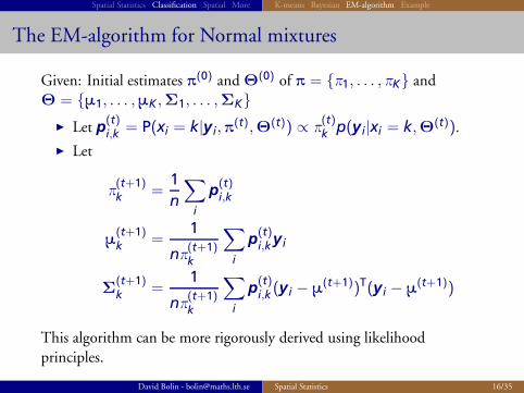
The EM-algorithm for Normal mixtures
Given: Initial estimates π(0) andΘ(0) of π = {π1, . . . , πK} and
Θ = {μ1, . . . ,μK,Σ1, . . . ,ΣK}
◮ Let p(t)i,k
= P(xi = k|yi,π(t),Θ(t)) ∝ π
(t)k
p(yi|xi = k,Θ(t)).
◮ Let
π(t+1)k
=1
n
∑
i
p(t)i,k
μ(t+1)k
=1
nπ(t+1)k
∑
i
p(t)i,k
yi
Σ(t+1)k
=1
nπ(t+1)k
∑
i
p(t)i,k(yi − μ
(t+1))T(yi − μ(t+1))
This algorithm can be more rigorously derived using likelihood
principles.
David Bolin - [email protected] Spatial Statistics 16/35
Spatial Statistics Classification Spatial More K-means Bayesian EM-algorithm Example
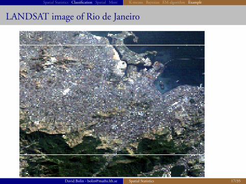
LANDSAT image of Rio de Janeiro
David Bolin - [email protected] Spatial Statistics 17/35
Spatial Statistics Classification Spatial More K-means Bayesian EM-algorithm Example
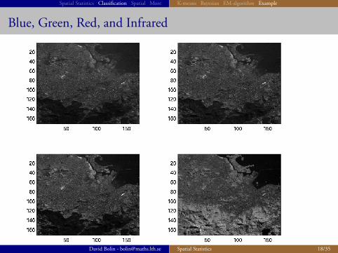
Blue, Green, Red, and Infrared
David Bolin - [email protected] Spatial Statistics 18/35
Spatial Statistics Classification Spatial More K-means Bayesian EM-algorithm Example
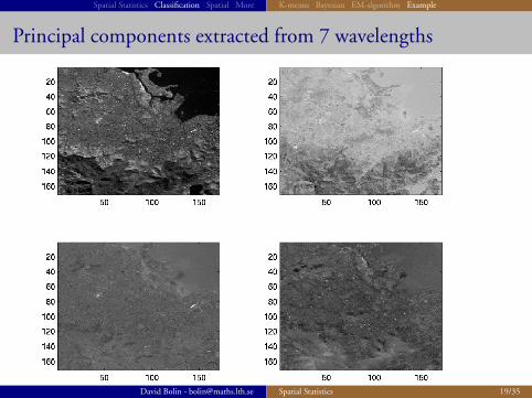
Principal components extracted from 7 wavelengths
David Bolin - [email protected] Spatial Statistics 19/35
Spatial Statistics Classification Spatial More K-means Bayesian EM-algorithm Example
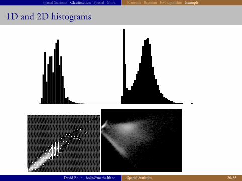
1D and 2D histograms
David Bolin - [email protected] Spatial Statistics 20/35
Spatial Statistics Classification Spatial More K-means Bayesian EM-algorithm Example
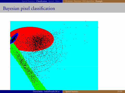
Bayesian pixel classification
David Bolin - [email protected] Spatial Statistics 21/35
Spatial Statistics Classification Spatial More K-means Bayesian EM-algorithm Example
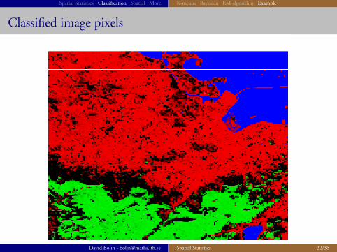
Classified image pixels
David Bolin - [email protected] Spatial Statistics 22/35
Spatial Statistics Classification Spatial More Reconstruction Ozone Temperature
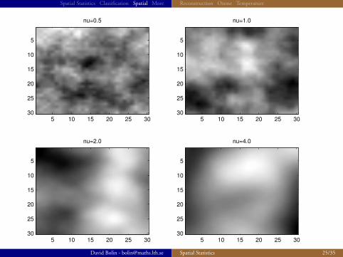
Stochastic fields
Many problems can be approached by modelling the spatial dependence
structure between pixels (or irregular locations).
◮ A random field is a collection of random variables x̃(u) with a
common density function.
◮ The random field can be used to model the dependence between
pixels, or other spatially varying data.
◮ For a random field x̃(u), the expectation function
mx̃(u) = E(x̃(u)) collects the point-wise expectations of the field.
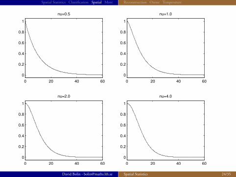
◮ For the covariance (dependence) between different pixels, we write
r(u,v) = C(x̃(u), x̃(v)) = E((x̃(u)− mx̃(u))(x̃(v)− mx̃(v))).
◮ r(u,v) is called the covariance function.
David Bolin - [email protected] Spatial Statistics 23/35
Spatial Statistics Classification Spatial More Reconstruction Ozone Temperature
0 20 40 60
0
0.2
0.4
0.6
0.8
1
nu=0.5
0 20 40 60
0
0.2
0.4
0.6
0.8
1
nu=1.0
0 20 40 60
0
0.2
0.4
0.6
0.8
1
nu=2.0
0 20 40 60
0
0.2
0.4
0.6
0.8
1
nu=4.0
David Bolin - [email protected] Spatial Statistics 24/35
Spatial Statistics Classification Spatial More Reconstruction Ozone Temperature
nu=0.5
5 10 15 20 25 30
5
10
15
20
25
30
nu=1.0
5 10 15 20 25 30
5
10
15
20
25
30
nu=2.0
5 10 15 20 25 30
5
10
15
20
25
30
nu=4.0
5 10 15 20 25 30
5
10
15
20
25
30
David Bolin - [email protected] Spatial Statistics 25/35
Spatial Statistics Classification Spatial More Reconstruction Ozone Temperature
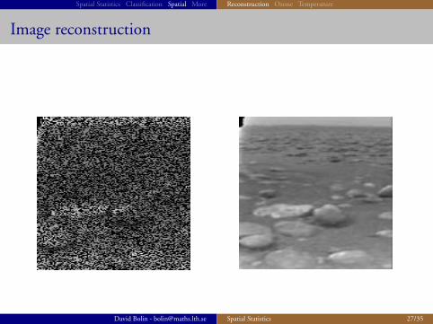
Image reconstruction
◮ Given an image with missing pixels we want to reconstruct the
missing values.
◮ Assume that the image is a sample from an underlying field.
◮ Estimate parameters of the field using the known pixels.
◮ Given parameters and data, estimate values for the missing pixels.
David Bolin - [email protected] Spatial Statistics 26/35
Spatial Statistics Classification Spatial More Reconstruction Ozone Temperature
Image reconstruction
David Bolin - [email protected] Spatial Statistics 27/35
Spatial Statistics Classification Spatial More Reconstruction Ozone Temperature
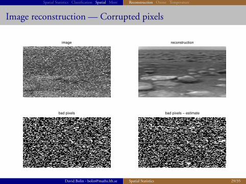
Image reconstruction — Corrupted pixels
◮ Typically we don’t know which pixels that are bad.
◮ A better model is then◮ Assume an underlying image, x.◮ Assume an indicator image for bad pixels, z.◮ Given the indicator we either observe the correct pixel value from x
or noise.
◮ Use Bayes’ Formula to compute the distribution for the unknown
image (and indicator) given observations and parameters.
◮ Estimate parameters and reconstruct.
David Bolin - [email protected] Spatial Statistics 28/35
Spatial Statistics Classification Spatial More Reconstruction Ozone Temperature
Image reconstruction — Corrupted pixels
image reconstruction
bad pixels − estimatebad pixels
David Bolin - [email protected] Spatial Statistics 29/35
Spatial Statistics Classification Spatial More Reconstruction Ozone Temperature
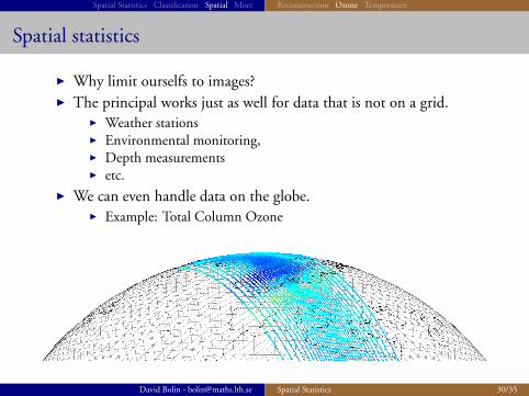
Spatial statistics
◮ Why limit ourselfs to images?
◮ The principal works just as well for data that is not on a grid.◮ Weather stations◮ Environmental monitoring,◮ Depth measurements◮ etc.
◮ We can even handle data on the globe.◮ Example: Total Column Ozone
David Bolin - [email protected] Spatial Statistics 30/35
Spatial Statistics Classification Spatial More Reconstruction Ozone Temperature
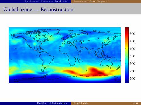
Global ozone — Reconstruction
200
250
300
350
400
450
500
David Bolin - [email protected] Spatial Statistics 31/35
Spatial Statistics Classification Spatial More Reconstruction Ozone Temperature
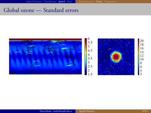
Global ozone — Standard errors
1.522.533.544.555.56
2468101214161820
David Bolin - [email protected] Spatial Statistics 32/35
Spatial Statistics Classification Spatial More Reconstruction Ozone Temperature
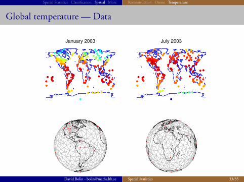
Global temperature — Data
January 2003 July 2003
David Bolin - [email protected] Spatial Statistics 33/35
Spatial Statistics Classification Spatial More Reconstruction Ozone Temperature
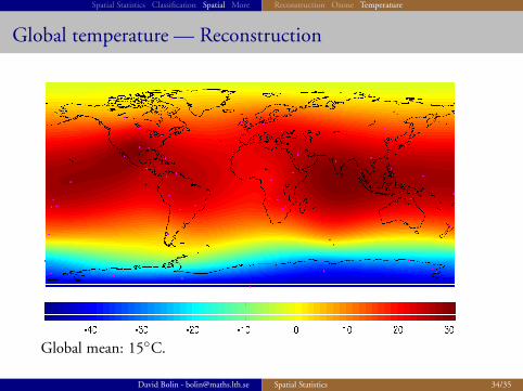
Global temperature — Reconstruction
Global mean: 15◦C.
David Bolin - [email protected] Spatial Statistics 34/35
Spatial Statistics Classification Spatial More
Learn more!
What?Spatial statistics with image analysis, FMSN20
When?HT2-2013, October–December
Where?Information and Matlab files will be available at
www.maths.lth.se/education/lth/courses/fmsn20masm25/
and
www.maths.lth.se/matstat/kurser/fmsn20masm25/
David Bolin - [email protected] Spatial Statistics 35/35


