
State Capacity and Economic Development: A NetworkApproach∗
Daron Acemoglu† Camilo García-Jimeno‡ James A. Robinson§
September 16, 2013
AbstractWe study the direct and spillover effects of local state capacity using the network of
Colombian municipalities. We measure local state capacity with the presence of state func-tionaries and institutions, and focus on its impact on local public good provision and pros-perity. We model the determination of local and national state capacity as a network game,in which each municipality, anticipating the choices and spillovers created by other munic-ipalities and the decisions of the national government, invests in local state capacity andthe national government chooses the presence of the national state in various areas to max-imize its own objective. We then estimate the parameters of this model, which reveal thedirect and spillover effects of local state capacity, both using reduced-form instrumental vari-ables techniques and structurally (using GMM, simulated GMM or maximum likelihood).Throughout our estimation, we exploit both the structure of the network of municipalities,regulating which municipalities create spillovers on which others, and the historical rootsof local state capacity as the source of exogenous variation for identifying both own andspillover effects. These are related to the presence of colonial royal roads and local presenceof the colonial state, factors which we argue are unrelated to current provision of public goodsand prosperity except through their impact on own and neighbors’ local state capacity. Ourestimates of the effects of state presence on prosperity are large. For example, bringing allmunicipalities below median to median state capacity, without taking into account equilib-rium responses of other municipalities, would increase the median fraction of the populationnot in poverty from 59.3% to 72%. Approximately 60% of this is due to direct effects and40% to spillovers. However, if we take the equilibrium response of other municipalities intoaccount, the median would instead increase to 78%, a very large change driven by equilibriumnetwork effects.
Very Very Preliminary and Incomplete. Please Do Not Circulate∗We are grateful to Alberto Ciancio, Amanda Culp, and Nicolas Idrobo for superb research assistance, and
Maria Angelica Bautista, Flavio Cunha, Frank Ditraglia, Elena Paltseva, Pascual Restrepo, Xun Tang, PetraTodd, Ken Wolpin, and participants at the Stockholm School of Economics/SITE conference on InstitutionalChallenges in Emerging Economies for valuable suggestions. Acemoglu gratefully acknowledges financial supportfrom ARO MURI.†Department of Economics, Massachusetts Institute of Technology. [email protected]‡Department of Economics, University of Pennsylvania. [email protected]§Government Department, Harvard University. [email protected]
1

1 Introduction
Though, in the West, we take for granted the existence of central and local states with the
capacity to enforce law and order, regulate economic activity and provide public goods, many
states throughout history and today in most less-developed parts of the world lack this capacity.
In Migdal’s (1988, p. 33) words: "In parts of the Third World, the inability of state leaders to
achieve predominance in large areas of their countries has been striking...”
The idea that such state capacity is vital for economic development, though latent in the
writings of Thomas Hobbes and Max Weber, began to attract more attention as a consequence
of analyses of the "East Asian Miracle”. A series of books by Johnson (1982), Amsden (1989) and
Wade (1990) argued that a key to the economic success of East Asian economies was that they
all had strong states. Evans (1995) developed this into a comparative theory of East Asian state
strength, arguing that it was the "embedded autonomy” of the South Korean state that made
it effective at promoting development. Others, such as Herbst (2000) and Centeno (2002) linked
the economic failure of African or Latin American nations to their limited state capacity1. This
hypothesis also receives support from the cross-country empirical evidence presented in Gen-
naioli and Rainer (2007) and the within-country evidence in Michalapoulos and Papaioannou
(2013) and Bandyopadhyay and Green (2012). All three papers find a positive impact of his-
torical measures of political centralization across African polities on contemporary public goods
provision and various measures of economic development. Relatedly, Boctstette, Chanda and
Putterman (2002) show a positive cross-country association between early state centralization
and economic development and Osafo-Kwaako and Robinson (2013) show similar correlations
using ethnographic data on political centralization from the Standard Cross-Cultural Sample.
Nevertheless, there is little convincing evidence for the impact of state capacity or “strength”
however conceptualized or measured, on economic development. What systematic empirical
findings there are, such as those of Evans and Rauch (1999, 2000), Besley and Persson (2009,
2011), and Dincecco and Katz (2013) show only correlations between measures of the extent to
which state officials are meritocratically recuited and promoted or the magnitude of tax revenues,
and measures of development. In all of these cases, as in the case study evidence above, it is
impossible to ascertain whether it is state capacity or some other institutional features that are
impacting public goods provision and economic development.1There is now a large monographic case study literature in political science and sociology on the role of state
capacity in economic development, for example Waldner (1999) and Kohli (2004)
1

In this paper, we contribute to this literature in several dimensions. First, we study the effect
of precise measures of state capacity of Colombian municipalities on public goods provision and
prosperity. We conceptualize "capacity" by the presence of state functionaries and institutions.
This represents one aspect of what Mann (1986, 1993) calls the "infrastructural power" of the
state (see Soifer, 2008). Colombia provides an ideal laboratory for this exercise both because
regional Colombian economic development is characterized by wide diversity in local state pres-
ence, public goods provision and prosperity, and because its history of colonization provides us
with sources of potential exogenous variation in state capacity which we exploit in order to deal
with potential endogeneity and reverse causality concerns and isolate the impact of state capac-
ity (rather than other social and institutional factors). In particular, we focus on the historical
presence of colonial state officials and the colonial “royal road” network. The road network, for
example, was partially based on pre-colonial indigenous roads and was largely replaced when the
modern system of roads was built in Colombia starting in the 1930s. This network has therefore
dissapeared, and thus (especially when we control for distance to current roads) provides an
attractive source of variation in the historical presence of the state, which is a key determinant
of the cost of building and expanding local state capacity. We exploit this royal road network as
well as information on the location of various colonial state offices in order to isolate historical
sources of variation in the costs of building state capacity today.
Second, to the best of our knowledge differently from all of the empirical literature in this area,
we explicitly allow for state capacity in one municipality to impact public goods provision and
economic outcomes in neighboring places. We expect (and empirically find) such neighborhood
externalities to be first order both because borders across municipalities are porous and because
building law and order or a functioning bureaucracy in the midst of an area where state capacity
is entirely missing is likely to be an insurmountable challenge2.
The potential impact of state capacity in one area on its neighbors, however, raises other
game-theoretic issues. Since building state capacity is costly (both because of political challenges
and because of the costs of building state agencies and hiring employees), municipalities may free
ride on the state capacity of their neighbors. Alternatively, there may be complementarities, and
municipalities may invest more in building state capacity when their neighbors are also doing so.
We tackle these issues by modeling the building of state capacity as a network game in which2For example, Di Tella and Schargrodsky (2004) show how a shock which led to increased policing in one part
of Buenos Aires reduced crime there but increased crime in neighboring parts.
2

each municipality takes the actions of the national government as well as their neighbors’ into
account and chooses its own state capacity. We then estimate the parameters of this structural
model exploiting both the network structure (following the ideas proposed in Bramoulle, Djeebari,
and Fortin, 2009) and the exogenous sources of variation discussed above. The key parameters
concern: (1) the impact of own state capacity on own public goods provision and prosperity; (2)
externalities on neighbors; and (3) the parameters of the best response equations revealing the
form of the dependence of municipalities’ decisions on building state capacity on their neighbors
decisions. In the process, we clarify why both empirical approaches that ignore the endogeneity
concerns and those that do not model the network structure of interactions will lead to misleading
estimates.
Our approach leads to precise estimates of the “best response” equations linking a munici-
pality’s state capacity to its neighbors, which show that in all cases state capacity decisions are
strategic complements. We estimate the effect of own and neighbors’ state capacity on various
measures of public goods provision (school enrolment, utilities coverage) and prosperity (quality
of life index and poverty) using one of three strategies: linear instrumental variables, generalized
method of moments and maximum likelihood. In each case, we make explicit how the reduced-
form parameters map into the structural ones. We find large and fairly precise effects of both
own and neighbors’ state capacity on these outcomes.
Our benchmark estimates imply, for example, that moving all municipalities below median
state capacity to the median will have a partial equilibrium direct effect (holding the level of state
capacity of all municipalities above the median constant) of reducing the median poverty rate by
12 percentage points, increasing the median coverage rate of public utilities (electricity, aqueduct
and sewage) by 17 percentage points, and increasing the median secondary enrollment rate by
25 percentage points. Our estimates suggest that about 60% of this is due to a direct effect,
while 40% is due to network spillovers. The full general equilibrium effect is very different,
however. Once we take into account the equilibrium responses to the initial changes in local
state capacity in the network, median coverage rate of public utilities increases 21 percentage
points, the median fraction of the population in poverty falls by 17 percentage points, and
median secondary enrollment rates increases by over 35 percentage points. These large impacts,
which are entirely due to network effects, highlight not only the importance of state capacity for
development but also the importance of taking general equilibrium effects into account.
We show that these estimates are quite robust. We end up with similar estimates with
3

or without controlling for the current road network, focusing on subsets of our instruments,
with different weights on different neighbors and under different assumptions on the reach of
externalities from neighbors.
We also extend our structural model to incorporate the decisions of the national government
concerning local state capacity. In particular, in Colombia, while municipalities themselves
hire and pay for a range of local state employees (large part of it with transfers from the central
government), the number of policemen and judges in the municipality are decided by the national
government. Incorporating this additional layer of interaction in the structural model has little
effect on our estimates, but allows us to estimate some key features determining the distribution
of national state presence across the country.
We are unaware of any other study that either estimates the effect of local state capacity
on local outcomes or models and estimates the network externalities and the network game in
this context. Nevertheless, our paper builds on and relates to several literatures. First, we build
on and extend the literature on the effect of state capacity on economic development which has
already been discussed above. In addition to the empirical and historical studies mentioned
above, there has recently been a small literature on the modeling of the emergence of state
capacity or persistence of weak states. Acemoglu (2005) constructs a model in which a self-
interested ruler taxes and invest in public goods and citizens make investment decisions. Lack of
state capacity or weak states are detrimental to economic development because they discourage
the ruler from investing in public goods as he anticipates that he will not be able to raise taxes in
the future. Besley and Persson (2009, 2010) also emphasize the importance of state capacity and
suggest that state building will be deterred when each group is afraid that the state they built
will be used against them in the future. Acemoglu, Ticchi and Vindigni (2011) and Acemoglu,
Robinson and Santos (2013) provide various models of persistence of weak states with low state
capacity. Our model takes a different direction than those and, in the process highlights a new
effect: state building will be deterred unless a national government plays an important role in this
process because local governments will underinvest in state capacity as they ignore the network
effects they create on their neighbors. Since our estimates suggest that these externalities are
substantial, this effect could be quite important in practice.
In utilizing a network game to model state building investments and for our empirical work,
our paper also relates to the literature on network games. Theoretically, our model is a variant of
Bramoulle, Kranton and D’Amours (2012), extended so that investments can be strategic com-
4

plements or substitutes (their model constrains them to be strategic substitutes). Empirically,
we build on Bramoulle et al.’s (2009) idea of using characteristics of neighbors and neighbors of
neighbors to overcome endogeneity within the network, but augment this with exogenous sources
of variation from the history of colonization in Colombia. Empirically, several of the issues we
confront in this paper are shared with the literature on peer effects (e.g., Calvo-Argemgol, Pat-
acchini, and Zenou (2009), Topa (2001), Katz, Kling, and Liebman (2001), Glaeser, Sacerdote,
and Scheinkman (1996), Bayer, Ross, and Topa (2008), Sacerdote (2002), and Nakajima (2007)).
Nevertheless, we are unaware of other studies that use a similar empirical strategy to estimate
the structural parameters of this type of model. In particular, we combine the use of moment
conditions derived from theory and identifying restrictions coming from the network structure,
to overcome the empirical challenges that emerge in this setting.
In addition to the literature we cited above on the role of state capacity in national economic
development, a small literature has emphasized, as we do, within-country variation in state
capacity. O’Donnell (1993) did this in the case of Latin America, arguing that the uneven
distribution of state capacity led to variation in the quality of democracy at the sub-national
level. Related ideas have emerged in the literature on civil wars with scholars arguing that
conflict starts and persists in parts of countries with low state capacity. Goodwin, for example,
argues that "revolutions are unlikely ... where the state effectively governs throughout the
national territory" (1999, p. 27). He also conceives of state effectiveness as infrastructural
power, in particular the territorial reach of the coercive capacity of the state through the national
territory. He argues that geographic areas where the state is ineffective provide spaces in which
revolutionaries can organize and evade repression3. Related ideas are widespread in the literature
on civil war (e.g., Fearon and Laitin, 2003, Kalyvas, 2006, and S·nchez, 2007, for the Colombian
case) but have not been rigorously tested. Research on within country income differences has
pointed at institutional differences as likely being a key explanatory variable (e.g. Acemoglu, and
Dell, 2010, Acemoglu, GarcÌa-Jimeno and Robinson, 2012, Bruhn and Gallego, 2012), but it has
not focused on variation in state capacity nor proposed an identification startegy. Most of the
empirical research in political science and sociology on the state has focused on the "first stage"
of our project in the sense that it has estimated models of the determinants of state capacity
rather than its consequences (e.g. Thies, 2005, 2007, Gennaioli and Voth, 2011, and Cardenas,3In the literature on state formation in the 19th century United States there is a heavy emphasis on the critical
role of federal and local government (e.g. Novak, 2008) and similar concerns have emerged in the literature onLatin America (see for example Soifer, 2012).
5
Eslava and Ramirez, 2011, for Colombia).
Finally, the network aspect of our paper is related to the literature on fiscal externalities be-
tween decentralized political units (Bewley, 1981, and Oates, 1999). Nevertheless, this literature
has not examined the types of externalities which are key to the current paper.
The rest of the paper proceeds as follows. Section 2 provides a discussion of the Colombian
context both regarding its colonial background as well as around the late 20th Century. Section 3
then presents a simple model of investments in state capacity within a network, Section 4 discusses
our empirical strategy, section 5 presents the data used in this paper, section 6 then presents our
reduced form and structural estimates and their implications, and section 7 concludes.
2 Context
This section provides a brief overview of some key features about the historical development of
state capacity in Colombia. Scholars of this country have long suggested that the weakness of the
state and its lack of spatial reach, has been a major source of the country’s poor development
experience and has contributed to its high levels of violence. The weakness of state presence
has been coupled since the 1886 Constitution by a high degree of Centralization at the national
level though this was reversed to some extent by the 1991 Constitution. Weak state presence
and strong centralization of state activity were also recurrent features of colonial Colombia, then
called Nueva Granada, during the three centuries of spanish colonial control.
The origins of this state weakness and absence are various. During the colonial period Spain
seriously restricted migration to its American colonies and after the huge populatiuon collapse
of the indigenous peoples in the century after conquest, they were concentrated into reducciones
(literally ’reductions’). Coupled to low population density were topographical challenges. The
Andean Cordillera running south to north splits in three close to the southern border with
Ecuador. The three mountain ranges, western, central, and easter, run north for around 600
miles effectively splitting the country into relatively disconnected regions both economically and
politically. But political factors also clearly influenced the nature, capacity, and presence of
the state. The Liberal regime that took power in 1850, for example, cut tariffs and abolished
monopolies in a way which created a fiscal crisis and led to severe state downsizing (Deas, 1982).
Since pre-colonial times, the highest population densities have been located in the highlands
of the Andes, particularly the eastern cordillera, and Spanish conquistadors and administrators
closely followed this pattern when settling during the 16th Century. Nevertheless, there were
6
significant changes in the distribution of the colonial state throughout the period of Spanish con-
trol, particularly after the beginning of the 18th Century when the Spanish under the Bourbons
attempted major institutional reform particularly directed at the strengthening of state control
in their American Colonies (see Paquette, 2012, Phelan, 1978, and McFarlane, 1993, for Colom-
bia). As the product of this set of reforms, the province of Nueva Granada became a viceroyalty
in 1717 and then again in 1739. Despite these efforts, the colonial state had a shallow presence
throughout the territory, and was highly spatially concentrated around a few cities and towns.
The Spanish never implemented the intended system of administration which was a key reform
used elsewhere in the Americas to strengthen the state. Bogota and Cartagena, as the capital
and the major slave and gold trading port, respectively, comprised 70% of all Crown employees
in the vicerroyalty in 1794.
The extractive nature of the Spanish colonial state naturally implied that its presence closely
followed economic resources. Most state activity was either focused on regulating gold mining,
particularly important in the western region, providing security services for the Spanish fleet
in the Caribbean, or attempting to regulate the relationship between settlers and indigenous
labor. These activities were very narrowly located in space, giving little incentive for the state
to develop a significant infrastructure or communications system. In fact, the only two attempts
at investing in infrastructure during colonial times were the water channel connecting the city of
Cartagena with the Magdalena river (which was at the time the only means of communication
and transportation from the Caribbean coast to the inland highlands), and the maintenance of
the royal roads network. In this paper, in fact, we exploit data related to the availability of this
royal roads network as a source of variation in historical state presence.
The royal roads network was the main investment in communications infrastructure during
the colonial period (the essays in Useche, 1995, provide detailed discussions of the royal roads
in many parts of Colombia). It was partially inherited from pre-colonial roads, and partially
built under Spanish authority. Pre-colonial roads often involved steep flights of steps unsuited
to horse or cart traffic (see Langebaek, Giraldo, Bernal, Monroy, and Barragan, 2000, for a
detailed study of the connections between pre-colonial and royal roads in eastern Colombia).
There is also archaeological evidence that indigenous roads were partly developed with religious
purposes, for pilgrimage to sacred places which were irrelevant to the Spanish. The difficulties
of converting colonial royal roads into modern motor roads were perhaps larger (see Pachon and
Ramirez, 2006, for a comprehensive overview). Some were still built for porterage along difficult
7

geographic paths, making them hard to subsequently reconvert to new transportation technolo-
gies. For example, although mountain edges were convenient for porter-based transportation of
merchandise, such road locations were inconvenient for railroads or highways. Historians and
Archaeologists agree that although the location of these roads reflect accurately the presence of
the colonial state, and the regions were the Spanish authorities were more interested in reaching
out an controlling the territory, most of the royal roads network was subsequently abandoned.
Around the mid 19th Century Colombia adopted a federal regime, that strengthened the
regional isolation and further weakened any attempts at national state-building. Indeed, each of
the states during this federal period had its own army, so that not even the Weberian idea of a
state having the monopoly of violence was attempted until the end of the War of 1000 days in
1903. Lack of centralization is acknowledged by Palacios and Safford as a major obstacle for the
development of the so needed communications infrastructure in this period. According to these
authors,
“In the decade of the 1870s, an attempt to use national funds to build a railroad that
would benefit the east triggered intense antagonism in the west and the [Caribbean]
coast... as a result, small, poorly financed and often failed projects proliferated...”
(Palacios and Safford ,2002, p. 27).
At the same time, the relative isolation of the different subregions (highland plateaus in the
Andes, valleys, etc.) also led to a relatively strong integration of nearby communities, and to a
relatively even distribution of political power between the disconnected regions. In their view,
the importance of local politics in Colombia has translated into a lack of centralized investments
that have limitted infrastructure development.
Palacios and Safford also provide some data that points to the extreme lack of state capacity
in the second half of the 19th Century. In 1870, with a total population of around 2.7 million,
the total number of both state and national level public employees was 4,500, or just 0.0015
bureaucrats per inhabitant! Some time later, in 1916 Palacios and Safford report 42,700 public
employees, for a population of 5.4 million, still only 0.0077 employees per capita. In comparison,
the U.S. during the Reagan administration had 0.072 public employees per capita, an order of
magnitude difference (Patton, 2013).
Throughout the 19th Century, another important phenomenon took place. In several regions
the relatively larger and wealthier cities during the Colonial era were leapfrogged by emerging
towns which had been relatively unimportant in that period. This is how in the Caribbean
8

coast Barranquilla grew rapidly while Cartagena stagnated and even saw its absolute population
decline. In the north-eastern Andes, the new cities of Cucuta and Bucaramanga surpassed the
colonial strongholds of Socorro, Velez and Pamplona. In the north-west, Medellin and Manizales
displaced Santafe de Antioquia as the largest and fastest growing urban centers. In the south,
Popayan was equally displaced by Cali. Interestingly, in our data we do find evidence that the
presence of the colonial state is negatively correlated with contemporary state capacity in the
same municipality, although colonial state presence in neighboring municipalities is positively
correlated with contemporary state capacity.
The capacity to raise fiscal revenues, one key aspect of state capacity, was also lacking all the
way into the 20th Century (as Deas, 1982, and Rincon and Junguito, 2007, note). For example,
commenting on this issue in 1912, Rufino Gutierrez argued that “...in most municipalities there
was no city council, mayor, district judge, tax collector... even less for road-building boards,
nor whom to count on for the collection and distribution of rents, nor who may dare collect the
property tax or any other contribution to the politically connected...” The independent state
basically inherited and for a long while left untouched the colonial fiscal system, which relied
mainly on indirect taxes: import tariffs, salt monopolies, and railway revenues.
State presence in Colombia continued to be weak throughout the 20th century. Robinson
(2013) interprets this as resulting from a form of ’indirect rule’ used by national elites to gov-
ern much of the country. As late as 1970 tax revenue was only around 5% of GDP (Rincon
and Junguito, 2007). In the different regions this has been interpreted as neglect from a very
centralized national government. Indeed, one of the main purposes of the 1991 Constitution,
as a demand from the regions, together with some policy attempts during the 80s to invest in
local state capacity (such as the Plan Nacional de Rehabilitacion), was to increase the extent of
descentralization in Colombia. The prevailing view was that descentralization would lead to a
strengthening of the state, through the local level. The logic behind this attempt was probably
that the weakness of state capacity in the regions could be substituted by local levels having more
direct control over public spending decisions. The 1991 Constitution in fact mandates transfers
from the central government to the local level. These transfers can only be used on specific areas
of public good provision, but in practice the spending decisions themselves are made by the
municipalities. Despite these major institutional changes in the late 20th Century, large swathes
of Colombia still have very weak state presence. Moreover, it was during the 1990s and early
2000s when the national state lost control of large peripheral areas of the country to the hands of
9

private armies of guerrillas and paramilitaries. In fact, even today some isolated regions as the
Choco or the Eastern Plains have not yet been at all integrated to the country. The reasons for
the failure of the reforms of the early 90s to alter the political equilibrium distribution of state
capacity are beyond the reach of this paper, but our findings may suggest some reasons for it.
3 A Simple Model of State-Building in a Network
In this section we develop a simple game-theoretic model of the determination of local and na-
tional state capacity, building upon the literature on games of public goods provision in networks.
Our starting point is the idea that the administrative map of a polity can be seen as a social
network were nodes are akin to the administrative units themselves, and links between nodes are
akin to the adjacency relations embedded in the map itself. Conveniently, in this perspective
links can be confidently considered fixed.
Thus, the economy consists of a network of municipalities, and a national state. Each munic-
ipality is a node of this network, municipalities sharing a border are connected, and we assume
throughout that all links are undirected. Prosperity in each municipality depends on local state
capacity, the spillover effects of state capacity from neighboring municipalities, and on national
state capacity allocated to the municipality. We further allow the strength of the spillovers to
depend on topographic features. All municipalities and the national state simultaneously choose
their levels of state capacity, to maximize their payoff, which is a function of the relative costs
and benefits of state capacity provision. State capacity positively impacts several dimensions of
prosperity, but its provision faces a convex cost. The national state, moreover, has heterogeneous
preferences over prosperity across municipalities. This simple model determines the equilibrium
distribution of local and national state capacity across municipalities, and hence the equilibrium
distribution of prosperity.
3.1 Network Structure and Preferences
Let i denote a municipality, and F be an n-x-n matrix with entries fij given by
fij =1
1 + δ1dij(1 + δ2eij)
where dij denotes the distance along the geodesic connecting the centroids of municipalities i and
j, and eij is a measure of variability in altitude along the geodesic connecting the centroids of
municipalities i and j. The fij ’s intend to allow for heterogeneity in the decay of any spillovers
10
between municipalities, depending on topographic features of the landscape. This will be an
especially relevant source of heterogeneity in the Colombian context due to the particularly
complex and rapidly variable topographic conditions of the country.
LetN(i) denote the set of municipalities connected to i. In practice we will consider adjacency
(two municipalities sharing a border) to imply a link. In our empirical exercises, nevertheless,
we experiment with alternative definitions of what constitutes a link, for example defining a link
to exist between any two municipalities within a certain distance of each other, or between not
only neighbors but also neighbors of neighbors. The matrix N(δ), on the other hand, denotes
the symmetric network matrix. Entry nij of this matrix is given by
nij =
{0 if j /∈ N(i)
fij if j ∈ N(i)
The network matrix captures both the presence of a link between two municipalities, and
the strength of any spillovers that may happen along that link. We allow several dimensions of
prosperity in a municipality to depend upon own state capacity and neighboring state capacity
in the following way:
pji = (κi + ξi)nisi + ψ1siNi(δ)s + ψj2Ni(δ)s + εji (1)
where pji is prosperity dimension j = 1, ...J in municipality i, si ∈ [0,∞) is municipality i’s state
capacity, ni is population, κi + ξi is the effect of own state capacity on prosperity, which we
allow to be municipality specific, and to depend on an observable κi and an unobservable (for
the econometrician) component ξi, ψ1 captures any interaction effect on own prosperity of own
and neighboring state capacity, and ψj2 captures the direct effect of neighboring state capacity
on own prosperity outcome j. Ni(δ) denotes the i’th row of the network matrix, and s denotes
the full column vector of state capacity levels. Finally εji are mean-zero unobservables for both
the municipality and the econometrician. We will rely on both direct measures of prosperity and
on measures of public goods provision.
3.2 The General Case
The most general model we consider allows state capacity in municipality i to be a constant
elasticity of substitution (CES) composite of both locally chosen li ∈ [0,∞), and nationally
chosen state capacity, bi ∈ [0,∞):
si =
[αl
σ−1σ
i + (1− α)bσ−1σ
i
] σσ−1
σ > 0 (2)
11

Each municipality decides its own state capacity li taking as given the choices of their neigh-
bors and the national government. Clearly, in the case α = 1, national choices are irrelevant.
Preferences for municipality i are assumed to take the form
Ui = Eε
1
J
∑j
pji −θ
2l2i
(3)
where J is the total number of prosperity outcomes. Preferences of the national level are assumed
to take the form
Wi = Eε
[∑i
{Uiζi −
η
2b2i
}](4)
where the ζi are the heterogeneous weights that the national state puts on each municipality.
It is interesting to note that though the focus of this paper is not to investigate the politics
of state building but rather to estimate the causal effect if state presence, there are several
ways we can think of politics entering into the model. For example, the parameters (κi, ξi) in
equation (1) capture the total factor productivity of state presence in municipality i. This will
be heavily dependent on politics. For example, if local politics is very clientelistic, as as the
case in Colombia (for example Davila and Leal, 2010) then many employees in the local public
payroll will be patronage appointments and this will create a situation with low total factor
productivity. Politics can also be thought of entering into the model via the weights ζi in the
objective function of the national level. For example, municipalities with many swing voters
might get a lot of weight because they are important places to gather votes, as in Stromberg
(2008).
We assume that local and national state capacities are chosen simultaneously. The first order
conditions for the municipalities and the national state determine the equilibria of this game.
Those with respect to li is given by
α
[sili
] 1σ
[(κi + ξi)ni + ψ1Ni(δ)s]− θli
{< 0 li = 0
= 0 , li > 0(5)
which is written in complementary slackness form. Given that (κi + ξi)ni ≥ 0, notice that only
if ψ1 < 0, can li = 0. The sign of ψ1 determines whether this is a game where local state
capacity choices are strategic substitutes (ψ1 < 0) or strategic complements (ψ1 > 0). Equation
(5) then implies that in a game of strategic complements, all municipalities will be providing a
positive level of state capacity in any equilibrium. Also notice that the overall externality from
neighboring state capacity on outcome j can be positive even in a game of strategic substitutes,
12

for large enough ψj2. Equation (5) is municipality i’s best response to all other municipalities’
and the national state’s choices.
For the national level, the first-order conditions with respect to each bi are given by
(1−α)
[sibi
] 1σ
{ζi [(κi + ξi)ni + ψ1Ni(δ)s] + ψ1Ni(δ)(s ∗ ζ) +
∑j ψ
j2
JNi(δ)ζ
}−ηbi
{< 0 bi = 0
= 0 bi > 0
(6)
where ∗ represents element by element multiplication. Notice from (6) that for any set of non-
negative weights ζ such that ζk > 0 for at least one k ∈ N(i) for all i, ψ1 > 0 and ψj2 > 0 for all
j is a sufficient condition for bi to be strictly positive in any equilibrium. In words, if spillovers
are positive and the game is one of strategic complements, the only way the national level could
allocate no state presence in municipality i is if municipality i’s weight, and all of municipality
i’s neighbors’ weights were zero. As we will describe below, our data on state capacity, both
local and national is strictly positive for all municipalities. This will allow us to focus on interior
equilibria.
Proposition 1: Sufficient conditions for a pure-strategy equilibrium of this game to exists
are either (i) ψ1 > 0 or ii) α < lσ+1σ
i sσ−1σ
i .
Existence of pure-strategy equilibria in this game follow either from the game exhibiting
strategic complementarities (ψ1 > 0) or from Kakutani’s fixed-point theorem and the concavity
of the payoff function in its own strategy (the strategy space can be assumed to be compact
by putting an arbitrary bound on state capacity). The inequality in Proposition 1 ensures that
the payoff function of municipality i is concave in its own strategy. If condition ii) above is not
satisfied, existence can still be guaranteed as long as the magnitude of the interaction effect ψ1
is small enough (See Appendix 1).
Regarding uniqueness, recent research by Allouch (2012) establishes that for network games
with non-linear best replies, a bound on the slope of the best responses is a sufficient condition
for existence and uniqueness. The bound is a function of the lowest eignevalue of the network
matrix N(δ). This is because the eigenvalues capture the extent to which the spillovers across
agents are either dampened or magnified through the network structure. Denote λmin as the
smallest eigenvalue of the network matrix N(δ).
Proposition 2: (Allouch (2012)). If for every player 1 + 1λmin(N(δ)) <
(∂li
∂Ni(δ)s
)−1< 1, the
game has a unique Nash equilibrium.
For an estimated parameter vector (α, σ, θ, ψ1, δ), the conditions in propositions 1 and 2 are
13

readily verifiable. Equations (1), (5) and (6) determine the joint equilibrium distribution of state
capacity, both local and national, and prosperity.
3.3 The Linear Case (α = 1):
The model above simplifies considerably in the case when α = 1, which reduces equation (2) to
si = li, so that the national level’s choices are irrelevant. In this case, the best reply equation
(5) becomes linear in neighboring state capacity provision:
sini
=ψ1
θ
Ni(δ)s
ni+κiθ
+ξiθ
(7)
Both in the general case and when α = 1, we specify κi as an unknown function of municipality
characteristics, and in particular, a function of historical state capacity characteristics which
we think of as shifters of the intercept of the best reply function. The work of Besley and
Persson (2010), for example, has stressed the idea that investments in state capacity are both
subject to large fixed costs and are long-lasting. As a result, it is likely that the Spanish colonial
state in Colombia has had a long-term effect on current state capacity levels. These historical
state presence measures, together with the network structure will be key to our identification
strategy. Equation (7) also highlights that even if properly identified, the interpretation of the
linear regression estimate of the “endogenous effect” (the effect of neighbors’ choice on own choice
in this context), should take into account that it is a reduced-form coefficient. It corresponds
neither to the interaction effect in equation (1) nor to the spillovers. Rather, it is the slope of
the best response function, and it is the quotient between the interaction effect and the elasticity
of the marginal cost of investment in state capacity.
We can additionally re-express the equilibrium state capacity from the best response equation
(7) as θsi = (κi+ξi)ni+ψ1Ni(δ)s, and substitute into the equation which determines prosperity
(1) to obtain
pji = θs2i + ψj2Ni(δ)s + εji (8)
Equation (8) shows that in equilibrium, the spillovers and feedbacks between municipality choices
within the network game imply a quadratic reduced-form relationship between own state capacity
and prosperity.
This result highlights the difficulty of estimating the relevant parameters using reduced-form
estimation. A regression of the relevant dependent variables on own and neighbors’ state capacity
will instead, at best, identify the parameter θ from variation in own state capacity, which is the
14

coefficient on the cost of state capacity investments, and has little to do with the actual effect
of own state capacity on the outcomes of interest (which is given by κi + ξi for municipality i).
Our empirical approach, detailed below, will overcome this difficulty as well.
With α = 1, existence of pure strategy equilibria follows immediately from concavity (and
Kakutani’s fixed point theorem as explained above) which always holds in this case. Uniqueness
of a positive equilibrium (where all municipalities choose a positive investment in state capacity)
is also guaranteed, since such an equilibrium is given by the solution to a set of linear equations.
However, multiple equilibria with some municipalities choosing zero investment is possible. A
condition for uniqueness of any equilibrium is given by Bramoulle, Kranton, and D’Amours
(2012) and can be applied directly here. Applying this condition and combining it with the
existence of equilibrium, we obtain:
Proposition 3: (Bramoulle, Kranton, and D’Amours (2012)). If |λmin(N(δ))| <(ψ1
θ
)−1,
the game has a unique Equilibrium.
This condition also ensures the equilibrium is stable. For an estimated parameter vector
(θ, ψ1, δ), the condition in proposition 3 can also be verified empirically.
Equations (7) and (8) determine the joint distribution of local state capacity and prosperity
across municipalities, and will be the focus of the first part of the paper. Identification of all
the key parameters (θ, ψ1, ψ2, δ) requires estimation of both equations. In equation (7), ψ1
θ
amounts to what is known in the literature on peer effects as an “endogenous effect”, while the
ψj2 ’s in equation (8) are what the literature on peer effects refers to as “contextual effects”. Of
course, the ξi and εji are likely to also include unobserved “correlated effects” (Manski, 1993),
and our empirical strategy will also tackle this problem.
4 Empirical Strategy
We aim to achieve several objectives with our empirical strategy. The first is to identify the
sign of the interaction effect in equation (1), which directly maps into the strategic nature of the
game being played between municipalities, and as a result, on the observed spatial patters of state
presence. Second, we would also like to characterize the relationship between several dimensions
of historical state presence and current state capacity choices. A priori this relationship could
have any sign. The Spanish colonial state made presence in several different dimensions, and
its objectives were likely to be heterogeneous across space. For example, in regions heavily
involved in gold mining during the 17th and 18th centuries, the presence of colonial officials
15

and Crown agencies was narrowly related to taxation purposes. In regions with higher densities
of Spanish settlers and their descendants, on the other hand, the demand for public services
such as legal adjudication and market regulation translated into a different type of colonial
state. Finally, in strategically located places the presence of the Spanish colonial state was
heavily related to military objectives. Moreover, given the at least partially extractive nature
of the Spanish colonial state in Colombia, the extent of its presence could well have had a
non-monotonic effect on the subsequent paths of local state building. Third, we are interested in
estimating the importance of state capacity on prosperity, both due to local choices and to spatial
spillovers. In particular, our estimation strategy will implicitly provide a test for the existence
of spillovers of this kind. Finally, we are also interested in providing a partial characterization of
the determinants of national state-building efforts, how they matter for public goods provision
and development, and how they interact with local choices.
Our structural model fully determines the equilibrium state capacity choices and prosperity
outcomes. Given the cross-sectional nature of our data and the strategic structure of our model,
we consider our data to reflect the resting point of a long-run process of standard best-response
dynamics. The conditions that ensure stability of this process and uniqueness of the equilibrium
depend on the slopes of the best replies and on the strength of the spillovers within the network.
For this reason, as noted above, we can directly verify these conditions given our empirical
estimates.4
Our data {(pi, li, bi,xi, ci)ni=1,D,E,A} used for estimation are cross sectional information
on several dimensions of prosperity pi, local li and national bi choices of state capacity, munic-
ipality characteristics xi, and colonial state presence characteristics ci. D, E, and A are n × n
matrices containing the geodesic distances between the centroids of all pairs of municipalities,
an index of variability in altitude along these geodesics, and the adjacecny status of each pair of
municipalities, respectively.
4.1 Linear Model
We propose several alternative estimation strategies. First, we assume that α = 1 which makes
equilibrium equations of our model (7) and (8) linear (in the reduced-form parameter ψ1
θ , and
θ and ψj2). As we argued above, we posit κiθ , the intercept of the best reply equation, to be an
4This leaves the question of whether for a different set of parameters there might be multiple equilibria and wemay incorrectly estimate a parameter vector implying uniqueness. We believe this is unlikely, since our estimatesare far from the values that would imply multiplicity.
16

unknown function of (ci,xi). Since we do not know the shape of this functional form, we will
allow for a flexible semi-parametric index-function approach for equation (7):
sini
=ψ1
θ
Ni(δ)s
ni+ g(ciϕ+ xiβ) + ςD + ξi (9)
where the ςD are department fixed-effects. For the purpose of estimating g() semi-parametrically,
we use a density estimator, by constructing the conditional expectation of the unknown function
using only the empirical distribution. To smooth out the distribution we use a density kernel
that gives weights to nearby observations to the point of evaluation. We use an index-function
approach due to the limited sample size. In practice, we divide the range of the function in many
bins5. Once the bin size is established we create a grid for the index, and assign a value for
the conditional expectation at the grid point from nearby observations, appropriately weighted
by the density kernel K(), and truncate the weighting at a specified distance of the grid point.
We experiment with both a biweight kernel and a normal kernel. For the linear model, the
conditional expectation is computed as follows:
E [g(ciϕ+ xiβ)] =
∑nj=1
[sjni− ψ1
θNi(δ)sni− ςD
]K((ci−cj)ϕ+(xi−xj)β
an
)∑n
k=1K((ci−cj)ϕ+(xi−xj)β
an
)where j are observations and i is the grid point.
In our estimating equations for the prosperity outcomes we include municipality characteris-
tics and department fixed effects:
pji = θs2i + ψj2Ni(δ)s + xiβj
+ ςjD + εji (10)
A first approach we pursue is to fix δ and let the function g() be approximated by a polino-
mial, as to be able to estimate (9) and (10) by linear regression. Nevertheless, there are several
identification challenges. The equilibrium implied by (9) means that Ni(δ)s is necessarily econo-
metrically endogenous in equation (1). This is the standard reflexion problem (Manski, 1993).
Because municipality j ∈ N(i) makes a choice which depends on si, Nj(δ)s =∑
k∈N(j) njksk is
a function of ξi, and thus, is correlated with ξi. This is true even if the ξi are pure idd noise6. If5For consistency, the bin size must satisfy two criteria: an → 0 as n→∞, and nan →∞ as n→∞. We also
make the bin size proportional to the index’s standard deviation to avoid having too many bins when the indexrange is very large. Following these rules, we choose an = 3.5std(ciϕ+ xiβ)n
− 13 .
6Solving for the social equilibrium in from (9), it is clear that each si is a function of all the ξj ’s:
s =ψ1
θN(δ)s+ n ∗ κ+ n ∗ ξ
17

ξi contains any unobservables that are common to i and j (correlated effects), the endogeneity
problem will be even more severe. Nevertheless, Bramoulle et al. (2009) show that the network
structure can provide valid instruments for Ni(δ)s. Their idea is relatively straightforward. If
for every node i there exists a node k such that k ∈ N(j), j ∈ N(i), and k /∈ N(i), then covariate
xk exactly satisfies the conditions for the validity of an instrument; it is correlated with the
endogenous regressor (cov(xk, sj) 6= 0) given that sj depends on sk which is a function of xk,
and it is not correlated with ξi (cov(xk, ξi) = 0). Indeed, the only way in which an exogenous
covariate of municipality k can have an influence on the state capacity choice of municipality i
is through the influence it has on municipality j’s choice of state capacity. This highlights that
if k ∈ N(i), xk will be an invalid instrument for si. Only the covariates of municipalities that
are neighbors of neighbors, but not themselves neighbors, will provide valid instruments.
In practice, the key difficulty with this approach is the assumption that xk is uncorrelated
with any unobserved correlated effects in ξi. This will be very likely for any covariates that are
spatially correlated, given that neighbor of neighbor municipalities will in general be relatively
close to each other. In the context of adolescent smoking choices, for example, suppose individuals
a and c are not friends, but have a common friend b. Parents’ education may influence own
smoking choices, and thus, c’s parents’ education may be proposed as an instrument to identify
how b’s smoking choices affect a’s smoking decision. Nevertheless, if both a and c live in a
neighborhood with a given sociodemographic profile, say high income, c’s parents’ education will
be picking up the effect of neighborhood prosperity on a’s smoking decision. In our setting,
there are several possible region-specific unobservables that may be correlated with neighbors
of neighbors observable municipality covariates. We thus propose to rely on detailed data on
the distribution of the Spanish colonial state which, as we will discuss in section 5 below, is in
practice very weakly or negatively spatially correlated. As we discussed in section 2, the colonial
settlement strategy implied the concentration of bureaucracies and agencies in particular cities,
which would have control and jurisdiction over surrounding areas. As such, towns with relatively
high levels of colonial state presence were likely to be surrounded by towns with relatively low
presence (See Figure 1, further described below). Moreover, the subsequent abandonment of
[I− ψ1
θN(δ)
]s = n ∗ (κ+ ξ)
s =
[I− ψ1
θN(δ)
]−1
n ∗ (κ+ ξ)
18

the royal roads network implies that although its proximity is a good reflection of colonial state
presence, these roads can confidently be considered unrelated to contemporary outcomes.
Denote by N2(i) the set of neighbors of neighbors of i that are not themselves i’s neighbors.
Thus, our first empirical strategy relies on using∑
k∈N2(i) fikck as instruments for Ni(δ)s in
equation (9). Our identifying assumption is thus that the colonial state presence level of munic-
ipality i’s neighbors of neighbors is uncorrelated with unobserved regional characteristics that
matter for prosperity, and that indeed municipalities in N2(i) are not connected with i. We use
this same set of instruments for Ni(δ)s in equation (10). In this equation, nevertheless, s2i is
also an endogenous regressor. By analogy, we use powers of Ni(δ)c as instruments for s2i . The
colonial state presence of the neighbors of municipality i should be correlated with i’s prosperity
only because i’s equilibrium choice of local state capacity depends on its neighbors’ local state
capacity choices.
System GMM
Separately estimating equations (9) and (10) is in general inefficient, given that the whole system
of J + 1 equations imposes several cross-equation restrictions due to their joint dependence on θ
and δ. Moreover, given our interest in estimating the shape of g(), we estimate equations (9) and
(10) as a system through a semi-parametric GMM approach inspired by Ichimura and Lee (1991).
These authors propose an index-approach semi-parametric non-linear least squares estimator. In
analogy to their methodology, by creating moment conditions coming from the orthogonality of
our instruments and the residuals in equations (9) and (10), we estimate the parameters of this
system through a semi-parametric GMM estimator. To identify δ we include as instruments
functions of dij and eij . In particular, we use the average distance of each municipality to
neighboring municipalities, and the average variation in elevation along geodesics connecting
municipality i to its neighbors. Let γ = (θ, ψ1,ψ2,ϕ,β, ς, β, ς). The estimator is given by
minγ,δ
[n∑i=1
Zi(δ)′qi(γ, δ)
]′( n∑i=1
Zi(δ0)′uiu
′iZi(δ0)
)−1 [ n∑i=1
Zi(δ)′qi(γ, δ)
](11)
where qi(γ, δ) = [ε1i , ..., εJi , ξi]
′, ui are residuals from a first stage estimate7, and
Zi(δ) =
[IJ ⊗ zpi (δ) 0
0 zBRi (δ)
]7ui = qi(γ0, δ0) and (γ0, δ0) = argminγ,δ
[∑ni=1 Zi(δ)
′qi(γ, δ)]′ (∑n
i=1 Zi(1)′Zi(1)
)−1 [∑ni=1 Zi(δ)
′qi(γ, δ)].
19

is the matrix of instruments for observation i. zpi (δ) is the vector of instruments for the prosperity
equations, and zBRi (δ) is the vector of instruments for the Best Response equation8.
4.2 General case
We subsequently relax the assumption that α = 1, allowing the national-level state capacity
choices to matter, and attempt to estimate the structural parameters of our full non-linear
model. We have several main objectives. First, to test whether allowing for the national-level
state capacity to matter for outcomes and for the strategic decision of municipalities (notice
that the bi shift the best reply functions of municipalities) alters our conclusions derived from
the restricted model. In particular, national-level choices could be both spatially correlated and
correlated with local state capacity choices in which case the estimates from the linear strategy
described above could be misleading. Second, it is also of interest to estimate the degree of
complementarity or substitutability between local and national state capacity in their effect over
prosperity.
Replacing the equilibrium conditions for the local state capacity choices, our structural equa-
tions (1), (5), (6) can be expressed as
hb(li,pi, bi|ζ) ≡ (1−α)
[sibi
] 1σ
{ζiθ
αli
[sili
]− 1σ
+ Ni(δ)
[(ψ1s +
∑j ψ
j2
Jι
)∗ ζ
]}−ηbi = 0 (12)
hξ(li,pi, bi) ≡θ
α
lini
[lisi
] 1σ
− ψ1Ni(δ)s
ni− g(ciϕ+ xiβ)− ςD (13)
hεj (li,pi, bi) ≡ pji −
θ
αlisi
[lisi
] 1σ
− ψj2Ni(δ)s− xiβj − ςjD (14)
where ι is a column vector of 1s, and with overall state capacity si defined by equation (2).
MLE with predetermined national choices
A first approach we pursue is to take the national-level’s choices as predetermined in the network
game between municipalities (this is, we ignore equation (12)). Our model thus reduces to equa-
tions (13) and (14). Conditional on the bi, these equations directly allow for a straightforward8The analytic asymptotic variance for this estimator is given by([
n∑i=1
Zi(ˆδ)′∇γ,δqi(ˆγ,
ˆδ)
]′( n∑i=1
Zi(δ0)′uiu
′iZi(δ0)
)−1 [ n∑i=1
Zi(ˆδ)′∇γ,δqi(ˆγ,
ˆδ)
])−1
20

maximum likelihood approach if we endow the εji ’s and the ξi with a joint distribution (and where
we still estimate the function g() semi-parametrically). The choice of estimator relies on the fact
that from equations (13) and (14) we can direcly invert the mapping from the endogenous vector
(li,pi) to unobservables (εi, ξi). In particular, we assume that
(ε1i , ..., εJi , ξi)
′ ∼ N(0(J+1)×1,Σ
)where
Σ =
σ2ε1 0 . . 0 00 σ2ε2 0 . . 0. . . . . .0 . . σ2
εJ0
0 0 . 0 σ2ξ
Define φ(εi, ξi; Σ) to be the joint density of (εi, ξi). Defining hξ(li,pi) ≡ hξ(li,pi|b), and
hεj (li,pi) ≡ hεj (li,pi|b), the likelihood for (li,pi) is given by9
Li(li,pi|b, l−i, ni, ci,xi;γ, δ,Σ) = φ(hε1(li,pi), ..., hεJ (li,pi), hξi(li,pi); Σ) |J i| (15)
where γ now includes α and σ. Finally, 10
|J i| =∂gξ∂li
=θ
α
1 + σ
σ
1
ni
[lisi
] 1σ
9Notice that hξ(li,pi) and hεj (li,pi) are one to one mappings:
∂hξ∂li
=θ
α
1 + σ
σ
1
ni
[lisi
] 1σ
∂hξ
∂pji= 0 ∀j
∂hεj
∂li= − θ
α
1 + σ
σsi
[lisi
] 1σ
∂hεj
∂pji= 1
∂hεj
∂pki= 0 for k 6= j
so that indeed we can invert the joint density as in (15).10
|J i| =
∣∣∣∣∣∣∣∣∣∣∣∣∣
∂hε1
∂li
∂hε1
∂p1i
∂hε1
∂p2i.
∂hε1
∂pJi∂hε2
∂li
∂hε2
∂p1i
∂hε2
∂p2i.
∂hε2
∂pJi
. . . . .∂hεJ
∂li
∂hεJ
∂p1i
∂hεJ
∂p2i.
∂hεJ
∂pJi∂hξ∂li
∂hξ∂p1i
∂hξ∂p2i
.∂hξ
∂pJi
∣∣∣∣∣∣∣∣∣∣∣∣∣=
∣∣∣∣∣∣∣∣∣∣∣∣∣∣
∂hε1
∂li1 0 . . 0
∂hε2
∂li0 1 0 . 0
. 0 0 1 . 0
. . . . . .∂hεJ
∂li0 0 0 . 1
∂hξ∂li
0 0 0 . 0
∣∣∣∣∣∣∣∣∣∣∣∣∣∣=∂hξ∂li
=θ
α
1 + σ
σ
1
ni
[lisi
] 1σ
21

Thus, the conditional MLE problem solves
maxγ,δ,Σ
{∑i
lnLi(li,pi|b, l−i, ni, ci,xi;γ, δ,Σ)
}(16)
Full Model (Simulated Method of Moments)
Our final empirical exercise consists of estimating the full model given by equations (12), (13), and
(14), which imposes the additional restrictions provided by the equilibrium choices of national-
level state capacity from equation (12). Of course, the national-level weights are unobserved.
We thus allow the importance given to municipality i to be a function of a vector of observable
characteristics related to within-network network position and importance, political variables,
and an unobserved component.
ζi = viπ + ωi (17)
We then define an average national-level choice first order condition as follows:
hb(li,pi, bi) =
ˆhb(li,pi, bi|ω)fω(ω)dω (18)
where fω() is the joint density of the national-level’s random weights. Notice that the
full vector of weights is assumed to be known to all players. Defining zNLi (δ) as a vec-
tor of instruments for the national-level’s best response equation, we propose a Simulated
Method of Moments estimator that takes the same form as (11), but with qi(γ, δ) =
[hε1(li,pi, bi), ..., hεJ (li,pi, bi), hξ(li,pi, bi), hb(li,pi, bi)]′, where
Zi(δ) =
IJ ⊗ zpi (δ) 0 00 zBRi (δ) 00 0 zNLi (δ)
and where the parameter vector γ now also includes η and π. In the empirical implementation
we test for the robustness of our estimator to several different densities fω().
5 Data
We compiled the data for this paper from several sources. The Fundacion Social (FS), a Colom-
bian NGO, collected and put together detailed data on state presence at the municipality level
in 1995, as measured by the presence of state agencies and bureaucracies. Out of a total of
1,103 municipalities in Colombia, FS collected data for 1,019. This constitutes the size of our
main sample, and the number of nodes in our network. Descriptive statistics for all of our
22

data are presented in Table 1 below. For each municipality, FS recorded the number of munic-
ipality (local) public employees, the number of national-level public employees, the number of
police inspections, police posts, courts, notary offices, Telecom offices,11, post offices, agricultural
bank offices12, public hospitals, public health centers, public health posts, public schools, public
libraries, fire stations, jails, culture houses, public instrument offices, and tax collection offices.
Because our theoretical framework stresses and exploits the difference between local and
nationally chosen levels of state capacity, we rely on the Colombian legislation to establish which
of the agencies for which FS has information are decided at the local level, and which at the
national level13. Police, courts, and public hospitals fall under the responsibility of the national
government. All other agencies are under the jurisdiction of the municipality. Because our
interest is closely related to the Weberian or “infrastructural” features of state capacity, and
not directly to the provision of public goods, we construct two measures of local state capacity
li: a) the number of municipality-level bureaucrats, which excludes police officers, judges, all
other judicial employees, and public hospital employees, and b) the total count of notary offices,
Telecom offices, post offices, fire stations, jails, public instrument offices, and tax collection
offices. We treat these two variables as alternative measures of local state capacity. We also use
the number of national-level public employees as our measure of national-level state capacity bi.
To measure local prosperity or development we collected available data from different sources.
The Centro de Estudios sobre Desarrollo Economico (CEDE) at Universidad de los Andes pro-
vided us with average 1992-2002 primary and secondary enrollment rates. From the OCHA
group at the United Nations, we collected data on aqueduct, sewage, and electricity household
coverage rates in 2002, and on vaccination rates in 2002. Finally, from the Colombian national
statistics bureau (DANE) we have data on the fraction of the population under the poverty line
in 1993 and 2005, and on a life quality Index for 1998. Based on these data, throughout our
empirical exercise we focus on four prosperity outcomes which are likely to depend on local state
capacity: a) the life quality index p1i , b) the average public utilities coverage in 2002 (aggregat-
ing aqueduct, sewage, and electricity) p2i , c) the population above the poverty line in 2005 p3i ,
and d) the secondary enrollment rate p4i . We focus on these four prosperity outcomes because11Telecom was the public telephone company at the time.12Caja Agraria.13Law 60 of 1993 and Law 04 of 1991 establish the distribution of responsibilities among the national and sub-
national levels in Colombia. The department level in Colombia was endowed by the 1991 Constitution with a verylimited number of responsibilities beyond mediating between the national and the municipal levels. Departments,nevertheless, can and do operate public hospitals.
23

although positively correlated between them, as Figure 2 shows, the shape of each distribution is
significantly different. Thus, we see each of these dimensions of prosperity as providing us with
relevant independent information.
In contrast, primary school enrollment and vaccination coverage are unlikely to depend on
local state capacity. Public investments targeting these outcomes are highly centralized in Colom-
bia. In fact, the Colombian Constitution mandates universal primary school enrollment. The
descriptive statistics in Table 1 show the very high average levels of primary enrollment, and the
small variation of this variable across municipalities. Moreover, the Ministry of Health directly
operates the vaccination efforts through national campaigns. In our robustness section below
we use these two development outcomes as a falsification exercise, showing their lack of relation
with the network structure.
To characterize our network we also directly built the adjacency matrix of Colombian mu-
nicipalities A based on the Colombian national geographic institute (IGAC)14. Using Arc-GIS
georeferenced data for Colombia, we also computed the geodesic (“as the bird flies”) distance
between the centroid of each pair of municipalities dij , and organize this data in matrix D. Also
using Arc-GIS and georeferenced topographic data for Colombia, we computed an index of the
variability in altitude along the geodesic connecting the centroid of every pair of municipalities
eij , and organize this data in matrix E. This variable is constructed by dividing each geodesic
in a number of intervals, each for a given altitude range along the geodesic itself, and computing
the average altitude of each of the intervals. The eij is then computed as the variance of the
average altitude across intervals, where each interval is appropriately weighted by its length. It
is intended to capture the frictions that a more uneven path should impose over the spillovers
across municipalities.
As discussed in the previous sections, we exploit variation in several dimensions of Spanish
colonial state presence in Colombia by using historical data originally collected by Duran y Diaz
(1794), an original source located at the National Library in Bogota that contains a full account
of state officials, salaries, the military, tariffs, taxes and fiscal revenue among others for all of the
Viceroyalty of Nueva Granada in the late 18th century.15 The document specifies the location of
officials and state administrations. Of particular interest, Duran y Diaz (1794) has a complete14We are excluding from our analysis the 2 municipalities in the Department of San Andres, which is an
archipielago in the Caribbean comprised of two major islands and several other smaller islands, and located at775 kms. from the mainland.
15We thank Malcolm Deas for pointing us to this document.
24

record of every colonial official and of several state agencies throughout the viceroyalty. From
this document we collected municipality-level data on the number of Crown employees, and
indicators on the presence of an alcabala16, a tobacco or playing cards estanco17, a liquor or
gunpowder estanco, and a post office. In addition to these variables we collected information
from historical maps in Melo and Moreno (2010) that depict the location of colonial royal roads.
We georeferenced these maps using Arc-GIS, and computed the distance between the centroid
of each municipality and the closest royal road. Based on this data we construct three measures
of colonial state presence: a) the number of Crown employees c1i , b) a count of the number of
agencies reported by Duran y Diaz18 c2i , and c) the distance to the closest royal road c3i .
In section 4 we argued that the validity of a strategy that relies on exploiting covariates
of neighbors of neighbors as instruments to identify social effects crucially depends on these
covariates not being correlated with any unobserved correlated effects. Although this is an
untestable assumption, it would be worrisome to find that the covariates used as instruments
are spatially correlated. Table 2 below presents the within-department spatial correlation matrix
of our three colonial state presence variables. The table presents the correlations between own
colonial state presence, neighbors’ colonial state presence, and neighbors of neighbors’ colonial
state presence.
The table shows a very low correlation of these colonial state presence measures between
adjacent municipalities and nearby municipalities. For example, distance to royal roads is the
variable with the highest spatial correlation. Nevertheless, own and neighboring distance to royal
roads has only a 0.28 correlation. This correlation falls to 0.045 between own and neighbors of
neighbors’ distance to royal roads. Own Crown employees are weakly negatively correlated
with neighbors’ and neighbors of neighbors’ crown employees (−0.061 and −0.062 respectively).
Similarly, own colonial state agencies are basically uncorrelated with neighbors’ and neighbors
of neighbors’ colonial state agencies (0.022 and 0.078 respectively). The patterns in Table 2
suggest that it is very unlikely that our historical measures of state presence will be picking up
unobserved correlated effects.
Finally we also use municipality-level covariates that include the distance to a current high-16The alcabala was a sales tax (usually 2%). The indicator denotes the presence of the local agency in charge
of collecting the tax.17An estanco was a state monopoly over the sale of a particular good, often including also a monopsony by
which the state regulated quantities and production rights. The indicator denotes the presence of the local agencyin charge of administering the estanco.
18Thus, this variable takes values in the set {0, 1, 2, 3, 4}.
25
way, longitude, latitude, surface area, altitude, average annual rainfall, and the density of pri-
mary, secondary, and tertiary rivers from CEDE, and the 1995 population from DANE. In
particular, to the extent that the location of contemporary and historical road networks may be
correlated, we find it especially important to control for the distance to current highways and
we do it throughout or estimation. As additional covariates, we also collected data from IGAC
on the distribution of land in each municipality by land quality (classified from quality 1 to 8),
by suitability (classified as agriculture-suitable, livestock-suitable, conservation-suitable), and by
land type (classified as under water, valley, mountain, hill, plain).
6 Results
In this section we present our estimates and empirical findings. As a preview, we find munic-
ipalities’ state-capacity investment decisions are strategic complements, and that the comple-
mentarity is weak enough that our parameter estimates are always consistent with the network
game having a unique and stable equilibrium. Our main finding is that various development
outcomes are strongly dependent on the overall levels of state capacity in a municipality, and
that state-capacity spillovers are significant. Quantitatively, own effects are about nine times as
large as spillover effects.
6.1 Linear Case
Our first set of estimates are obtained from a model where we assume that α = 1 and thus we
focus our attention on the game between municipalities. In this case, the best replies are linear,
and the data generating process is fully determined by equations (9) and (10) above. Table 3
presents the estimates for equation (9), where we measure state capacity alternatively as the
number of public agencies (columns 1-3) or the number of municipality employees (colmns 4-6).
Columns 1 and 4 present an OLS benchmark, where we impose δ = (1, 1) and we assume g()
is a linear function: g(ciϕ + xiβ) = a + ciϕ + xiβ. All reported values are average marginal
effects for ease of comparison19. Columns 2 and 5 then present instrumental variables estimates
for the same equation, where we rely on the Bramoulle et al (2009) strategy described in section
4. As instruments for neighboring state capacity Ni(δ)s we use neighbors of neighbors colonial
officials, colonial agencies, and distance to royal roads. Estimates for the first stage of this model
are presented in the bottom panel of Table 3. Finally, columns 3 and 6 present our main GMM19Standard errors for these marginal effects are computed using the delta method.
26

estimates where we estimate equations (9) and (10) as a system (equation (10) is estimated
for each of our four prosperity outcomes described in section 5), the function g(ciϕ + xiβ) is
estimated semi-parametrically, and the parameter δ is also estimated in this case.
First, notice that the conditions for a unique equilibrium in Proposition 3 are easily satisfied
at our parameter estimates. At our GMM estimates, when measuring state capacity through
agencies, we have (ψ1/θ)−1 = 0.4301 > λmin(N(δ)) = 0.2356. When measuring state capacity
through local bureaucracies, we have (ψ1/θ)−1 = 0.5284 > λmin(N(δ)) = 0.2357. The condition
is also satisfied at the OLS and IV estimates.
All of our estimates in Table 3 show a positive and very precisely estimated slope for the
best reply equation, also implying a positive interaction effect ψ1. These estimates imply that
the game between municipalities exhibits strategic complementarities. The 0.076 (s.e. 0.013)
estimate in the top of column (3) implies that at the median number of local state agencies
in our sample, one neigbor’s number of state agencies moving from the median (10) to the
mean (21) would lead to a 2.2% increase in own state agencies20. Notice this is only the direct
(immediate) response, and does not take into account equilibrium feedbacks would take place
through network effects as other municipalities also respond (due to strategic complementarities).
Given that the median number of neighbors is 5, this same immediate effect could be achieved
if all five neighbors increased their number of state agencies by 2. In that case, though, the
subsequent indirect effects would be different.
Figure 1 below presents our estimated function g(ciϕ+xiβ) from the system GMM. Through
most of the relevant range, the function is very precisely estimated. Recall that in our model,
gi(.) =κiθ, is proportional to the average effect of own state capacity on prosperity. The figures
show that the function is positive for all its relevant range and is increasing non-linearly. This
result highlights the importance of estimating g(ciϕ+ xiβ) flexibly, and suggests that the effect
of own state capacity on prosperity is quite heterogeneous across municipalities. Table 3 also
presents the average marginal effects ϕg′(ciϕ + xiβ) for the historical state presence variables,
revealing that overall, own colonial state officials and state agencies have a negative effect on
own contemporary state. At the same time, the bottom panel reveals a strong and positive effect
of neighbors of neighbors’ colonial state agencies on neighbors’ contemporary state capacity, and
a strong and negative effect of neighbors of neighbors’ distance to royal roads on neighbors’
contemporary state capacity.20(0.076) ∗ [ln(21)− ln(10)] = 0.056, which is 2.2% of the baseline log state capacity
27

Our key structural parameters resulting from the estimation of equation (10), are presented
in Tables 4 and 5. Similarly to the estimates reported for equation (9), we present benchmark
OLS and IV results from estimating each of our four prosperity outcomes separately (columns
1, 2, 4, 5, 7, 8, 10, and 11), and subsequently present the system GMM estimates in columns 3,
6, 9, and 12. Table 4 presents the estimates for the models using the number of agencies, and
Table 4B presents the estimates for the models using the number of municipality employees. In
all cases, we find both strong own effects that are quite significant and also even more precisely
estimated spillover effects. The quantitative magnitudes of the estimates are very similar between
Tables 4 and 5. Notice that the simultaneous-equations estimation increases the precision of our
estimates.
To assess the quantitative magnitudes of these estimates, as a first counterfactual exercise
Table 5A shows the implications of increasing all municipalities below median state presence to
the median. The first panel shows the partial equilibrium effects (holding the response of other
municipalities constant). We see quite significant increases in the Life Quality Index, the fraction
of the population not in poverty, utilities coverage and secondary enrollment. For example, the
fraction of the population not in poverty increases from 59.2% to 72%. The table also indicates
that about 63% of this is due to direct effects, so that spillover effects are not implausibly large,
though still sizable. The second panel then factors in the equilibrium responses through network
effects. Now the quantitative magnitudes are much larger. For example, fraction not in poverty
now rises to 78%. Of course, in this case, the additional sizable impact is due to the network
effects, which trigger responses from all municipalities through strategic complementarities. In
fact, the general equilibrium experiment also shows that nudging the level of state capacity of
all municipalities below median by taking them to the median (which leaves the median of the
distribution unchanged at the time of the experiment), leads, after the general equilibrium social
interactions in the network have happened, to a shift in the median of the distribution of state
capacity from 10 to 22.5. In fact, the final equilibrium distribution of state capacity compresses
considerably with the experiment, as the median and the mean are now very similar.
To investigate the sensitivity of our estimates in Tables 4 and 5 to the quadratic form on
si, we present OLS and IV results of running a misspecified model where own state capacity
enters linearly. Table 6 presents the estimates of this “naive” regression. Though this equation is
potentially misspecified, the estimates are still significant and quantitatively similar, which we
find reassuring as it also implies that functional forms are not responsible for our main structural
28

estimates. Compare, for example, the IV marginal own effects from Table 4 with those from Table
6. Measuring state capacity with agencies, the estimate in Table 4 are between 0.49 and 0.28,
while those in Table 6 are 0.36 and 0.25.
Figure 4 presents graphic evidence illustrating the fit of the model estimated by system
GMM. It shows scatterplots with the observed and predicted values for state capacity (measured
as number of bureaucrats) and prosperity outcomes using the estimated parameters in column
6 of Table 3, and columns 3, 6, 9, and 12 of Table 4B. The fit is very similar when measuring
state capacity through local level agencies.
The scatterpolots in Figure 4 show that the linear specification does a great job at predicting
all of the endogenous variables in the model. Nevertheless, they do show that the model does
a somewhat less satisfactory job for the tail of the distribution of both state capacity levels
and prosperity, where it tends to over-predict. (These are the largest and more prosperous
municipalities.) This result leaves the door open for the general version of the model to provide
a better fit of the tail of the distribution.
As we mentioned in section 5, there are some development outcomes (primary enrollment and
vaccination coverage) that closely depend on national-level policies in Colombia. As such, we
would expect local state capacity not to be significantly correlated with these outcomes. Table
7 below presents OLS and IV estimates of equation (10) for these two outcomes as a “placebo”
exercise. As the table ilustrates, we find them not to be correlated at all with either own or
neighboring local state capacity.
We also find that the results reported so far are robust. Here, to save space, we present only IV
estimates of equation (10) for our four prosperity outcomes. In Table 8A we estimate the model
without controlling for the distance to a current highways (Panel I), and introducing additional
geographic covariates (Panel II). Among the additional covariates we include the density of
primary, secondary and tertiary rivers, and the full distribution of land by qualities, suitability,
and type as described in section 5. All estimates remain pretty much unchanged compared
with those of Tables 4 and 5, except for the marginal own effect on secondary enrollment when
measuring state presence with municipality employees, in the exercise where we control for the full
set of additional geographic covariates (column (8) of Panel II on Table 8A). Notice, nevertheless,
that this is the outcome for which we have the smallest sample size, and in this specification
we are introducing seventeen additional controls. Moreover, the estimated marginal neighbors’
effect remains unchanged in this specification.
29

Table 8B then presents robustness exercises related to the network structure itself. In Panel I
we use third-degree neighbors colonial state covariates as instruments instead of our benchmark
second-degree neighbors colonial state. In Panel II we present the results of redefining the
meaning of a link, by considering either adjacent or second-degree adjacent municipalities as
connected. We consider the robustness exercises in Table 8B of great importance because we do
not know for certain what the true network structure is. Rather, in our benchmark especification
we are making the assumption that links are given by adjancency. Although a natural one, this
is still an assumption. The results of Table 8B show that our estimated effects are robust to
changing our assumptions about the network structure.
Finally in Table 8C we look at the sensitivity of our estimates to using subsets of our colonial
state presence instruments. In Panel I we exlude all functions of distance to royal roads from
the instrument set, and in Panel II we exclude all functions of colonial state employees from
the instrument set. This is akin to an overidentification test, since significantly different IV
estimates coming from different subsets of the instrument set would suggest that the identification
assumption is invalid for some of the instruments. The table illustrates the stability of our
estimates across subsets of instruments.
More importantly, we also consider the effect of controlling for the national-level bureaucracy,
on our estimates of both the best reply and the prosperity equation. This is important since
we would like to rule out that local state capacity is simply proxying for national-level state
capacity. Table 9 presents the IV results for the best reply, and Table 10 the IV results for
the prospserity outcomes equations. If anything, controlling for the national-level bureaucracy
increases the precision of our estimated effects.
We are also concerned with the possibility of heterogeneity across municipalities in their
objective function. In the Colombian context, illegal armies have contested state authority for
several decades, and local elites that successfully control local politics may well have objectives
that differ from what we posited in equation (3) where the marginal cost of providing state
capacity is constant across municipalities. We investigate the possible confounding effects of this
kind of heterogeneity by re-estimating our model excluding from our sample or from the network
itself, municipalities with historically high levels of violence as measured by paramilitary and
guerrilla attacks during the 1998-2004 period. Specifially in Panel I of Table 11 we exclude from
the estimating sample (but not from the network), municipalities above the 90th percentile of
the either the distribution of paramilitary or of guerrilla attacks. In Panel II we exclude this
30

same subset of municipalities from the network. The table presents the IV results, and illustrates
the robustness of our benckmark specification.
6.2 General Case
Our second set of main results relaxes the assumption that α = 1, allowing both for the national-
level state presence to matter for prosperity, and for the national government to be a player in
the state-building game. In this case, best replies are no longer linear and thus we implement two
alternative estimation strategies. First, we leave the national-level choices b as pre-determined,
and estimate equations (13) and (14) by conditional maximum likelihood as described in section
4.2. We then also model the national-level’s choices. In this case the national level’s first order
condition for each bi depends nontrivially on the full vector of weights ζ. Thus, we use this first
order condition to build moment conditions and simulate the moment by assuming a distribution
for the ω’s. We thus estimate the full system (12)− (14) through Simulated GMM.
We present our structural parameter estimates for the first exercises in Table 12, and based on
them perform a series of counterfactual exercises that take into account the general equilibrium
interactions taking place within the network game. These allow us to answer relevant questions
of interest. The first column of the table presents the estimates when we use the number of
state agencies as our measure of state capacity, and the second column presents the estimates
when using the number of municipality employees. We find a relatively high weight for local
state capacity within the CES composite (α of around 0.7). Moreover, the estimated elasticity
of substitution between local and national state σ is estimated to be relatively high, implying
that the CES composite is actually not far from linear in l and b, and a relatively large degree
of substitution between both types of state presence but also little strategic dependence of local
on national state. The structural estimate for the interaction effect ψ1 also directly implies
the strategic complementarity that we found in our linear model. The table also presents the
average (across the sample of municipalities) value of κi, which we recover in our estimation as
κi = θg(ciϕ+ xiβ). The table presents the standard deviation of the estimated κi’s. Recall κi
is proportional to the direct effect of own state capacity on prosperity.
At the parameter estimates in Table 12, the condition for uniqueness from Proposition 2 is
easily satisfied both when estimating the model for state agencies and for municipality employ-
ees. In the former case, we have that λmin(N(δ)) = −0.075, and 1 + 1λmin(N(δ)) = −12.35 <
min
{(∂li
∂Ni(δ)s
)−1}= 0.15 < max
{(∂li
∂Ni(δ)s
)−1}= 0.177 < 1, and in the latter we have
31
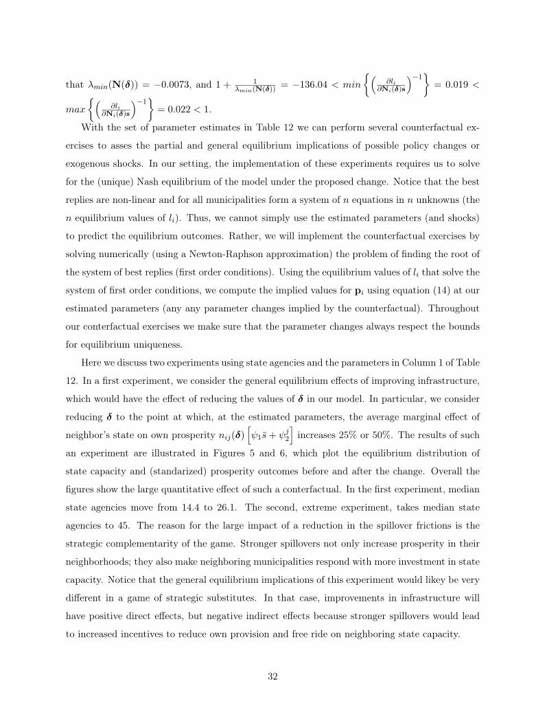
that λmin(N(δ)) = −0.0073, and 1 + 1λmin(N(δ)) = −136.04 < min
{(∂li
∂Ni(δ)s
)−1}= 0.019 <
max
{(∂li
∂Ni(δ)s
)−1}= 0.022 < 1.
With the set of parameter estimates in Table 12 we can perform several counterfactual ex-
ercises to asses the partial and general equilibrium implications of possible policy changes or
exogenous shocks. In our setting, the implementation of these experiments requires us to solve
for the (unique) Nash equilibrium of the model under the proposed change. Notice that the best
replies are non-linear and for all municipalities form a system of n equations in n unknowns (the
n equilibrium values of li). Thus, we cannot simply use the estimated parameters (and shocks)
to predict the equilibrium outcomes. Rather, we will implement the counterfactual exercises by
solving numerically (using a Newton-Raphson approximation) the problem of finding the root of
the system of best replies (first order conditions). Using the equilibrium values of li that solve the
system of first order conditions, we compute the implied values for pi using equation (14) at our
estimated parameters (any any parameter changes implied by the counterfactual). Throughout
our conterfactual exercises we make sure that the parameter changes always respect the bounds
for equilibrium uniqueness.
Here we discuss two experiments using state agencies and the parameters in Column 1 of Table
12. In a first experiment, we consider the general equilibrium effects of improving infrastructure,
which would have the effect of reducing the values of δ in our model. In particular, we consider
reducing δ to the point at which, at the estimated parameters, the average marginal effect of
neighbor’s state on own prosperity nij(δ)[ψ1s+ ψj2
]increases 25% or 50%. The results of such
an experiment are illustrated in Figures 5 and 6, which plot the equilibrium distribution of
state capacity and (standarized) prosperity outcomes before and after the change. Overall the
figures show the large quantitative effect of such a conterfactual. In the first experiment, median
state agencies move from 14.4 to 26.1. The second, extreme experiment, takes median state
agencies to 45. The reason for the large impact of a reduction in the spillover frictions is the
strategic complementarity of the game. Stronger spillovers not only increase prosperity in their
neighborhoods; they also make neighboring municipalities respond with more investment in state
capacity. Notice that the general equilibrium implications of this experiment would likey be very
different in a game of strategic substitutes. In that case, improvements in infrastructure will
have positive direct effects, but negative indirect effects because stronger spillovers would lead
to increased incentives to reduce own provision and free ride on neighboring state capacity.
32

A second experiment of interest asks about the role of national-level state presence. Given
it’s large variability across municipalities, we look at the general equilibrium effects of taking all
municipalities below median national-level public employees bi to the median. The results of this
exercise are presented graphically in Figure 7. In this case, the magnitude of the effects is smaller,
but still positive and of economic relevance. Median local state agencies increase from 14.4 to
15.2, leading to a 12% increase in the median Life Quality Index, a 8.7% increase in median
Public Utilities coverage, a 12.5% increase in the median fration of population above the poverty
line, and an 11% increase in median secondary enrollment rates. The reason for this more limited
effects of a shock to national-level state presence is that we are estimating a relatively low weight
of bi in the state capacity composite, together with a relatively high elasticity of substitution
between locan and state investments. Given the low weight of bi in the CES composite, the
direct effect of bi on prosperity is small. Moreover, the relatively high elasticity of substitution
implies that the strategic response of municipalities to increased national-level state is relatively
weak, leading to a small indirect effect.
Our results and experiments highlight the importance of centralized state-building in a con-
text where investments across neighboring communities are strategic complements. Within a
highly fragmented country like Colombia, where economic ties between regions are fairly limited,
our conterfactual exercises emphasize the high costs of uncoordinated investments that ignore
positive spillovers. More importantly, they emphasize that strategic complementarities increase
the value of centralized or coordinated decisionmaking.
7 Conclusions
In this paper we develop a framework for estimating the direct and spillover effects of local
state capacity using the network of Colombian municipalities. We propose measuring local state
capacity with the presence of state functionaries and institutions, and focus on its impact on local
public goods provision and prosperity. We model the determination of local and national state
capacity as a network game, in which each municipality, anticipating the choices and spillovers
created by other municipalities and the decisions of the national government, invests in local state
capacity and the national government chooses the presence of the national state in various areas
to maximize its own objective. We then estimate the parameters of this model, which reveal the
direct and spillover effects of local state capacity, both using reduced-form instrumental variables
techniques and structurally (using GMM, simulated GMM or maximum likelihood). In all of our
33

estimations, we exploit both the structure of the network of municipalities, determining which
municipalities create spillovers on which others, and the historical roots of local state capacity as
the source of exogenous variation for identifying both own and spillover effects. These are related
to the presence of colonial royal roads and the historical presence of the colonial state, factors
which we argue are unrelated to current provision of public goods and prosperity except through
their impact on own and neighbors’ local state capacity. We find large effects of state presence
on prosperity, and that network effects are first order. For example, bringing all municipalities
below median to median state capacity, without taking into account equilibrium responses of
other municipalities, would increase the median fraction of the population above the poverty line
from 59.3% to 65.3%, approximately 90% of this due to direct effects and 10% due to spillovers.
However, if we take the equilibrium responses of other municipalities into account due to the
strategic complementarity of municipalities’ choices, the median of the fraction of the population
not in poverty would instead increase to 79.2%, a very large change driven by equilibrium network
effects.
We view our paper as a first step in the modeling and estimation of the direct and spillover
effects of local state capacity, an in estimating general equilibrium social interactions within a
network. Our framework and estimates point to several issues that have not been emphasized in
the literature and that require further investigation. First, our results indicate a major obstacle
to the building of state capacity pioneered by local authorities: each municipality will tend to
ignore its positive effects on others, leading to underinvestment in local state capacity. This leads
to a new argument for why state centralization and building of state capacity often go hand-in-
hand. Second, our results focus only on some aspects of local state capacity. The typical view of
the Weberian rational bureaucracy also emphasizes such things as meritocracy and predictability
of the bureaucracy, which would be interesting to investigate at the local level too. Thirdly and
more importantly, we have stayed away from another aspect of Weberian state capacity, the
monopoly of violence. This is a central issue in Colombia, both as part of how the local state
functions and one of its main implications (e.g., homicides, activities of private armies). This is
an area of future research for us and for others.
8 References
Acemoglu, Daron (2005). “Politics and Economics in Weak and Strong States”, Journal of
Monetary Economics, 52, 1199-1226.
34

Acemoglu, Daron and Melissa Dell (2010). “Productivity Differences Between and
Within Countries,” American Economic Journal: Macroeconomics, 2(1), 169–188.
Acemoglu, Daron, Camilo García-Jimeno and James A. Robinson (2012). “Find-
ing El Dorado: Slavery and Long-Run Development in Colombia,” Journal of Comparative Eco-
nomics, 40(4), 534-564.
Acemoglu, Daron, James A. Robinson and Rafael J. Santos (2013). “The Monopoly
of Violence: Theory and Evidence from Colombia,” Journal of the European Economic Associa-
tion, 11(1), 5-44.
Acemoglu, Daron, Davide Ticchi and Andrea Vindigni (2011). “Emergence and
Persistence of Inefficient States” Journal of the European Economic Association, 9(2), 177-208.
Allouch, Nizar (2012). “On the Private Provision of Public Goods on Networks”, Unpub-
lished.
Amsden, Alice H. (1989). Asia’s Next Giant: South Korea and Late Industrialization,
New York: Oxford University Press.
Ballester, Coralio and Antoni Calvo-Armengol (2010). “Interactions with Hidden
Complementarities”, Regional Science and Urban Economics 40, 397-406.
Ballester, Coralio, Antoni Calvo-Armengol, and Yves Zenou (2006). “Who’s who
in Networks: Wanted: The Key Player”, Econometrica, 74(5), 1403-1417.
Bandyopadhyay, Sanghamitra and Elliot D. Green (2012). “Pre-Colonial Political
Centralization and Contemporary Development in Uganda”, APSA 2012 Annual Meeting Paper.
Bayer, Patrick, Stephen Ross, and Giorgio Topa (2008). “Place of Work and Place
of Residence: Informal Hiring Networks and Labor Market Outcomes”, Journal of Political
Economy, 116(6), 1150-1196.
Besley, Timothy and Torsten Persson (2010). “State Capacity, Conflict, and Develop-
ment”, Econometrica 78(1), 1-34.
Besley, Timothy and Torsten Persson (2009). “The Origins of State Capacity: Property
Rights, Taxation and Politics”, American Economic Review, 99(4), 1218-44.
Besley, Timothy and Torsten Persson (2011). Pillars of Prosperity, Princeton: Prince-
ton University Press.
Bewley, Truman (1981). “A Critique of Tiebout’s Theory of Local Public Expenditures”,
Econometrica, 49(3), 713-740.
Blume, Lawrence, William Brock, Steven Durlauf, and Yannis Ioannides (2010).
35

“Identification of Social Interactions”, in J. Benhabib, A. Bisin, and M. Jackson (eds.). Handbook
of Social Economics (Forthcoming).
Bockstette, Valerie, Areendam Chanda and Louis Putterman (2002). “States and
Markets: The Advantage of an Early Start”, Journal of Economic Growth, 7: 347-69.
Bramoullé, Yann and Rachel Kranton (2007). “Public Goods in Networks”, Journal
of Economic Theory, 135, 478-494.
Bramoullé, Yann, Rachel Kranton and Martin D’Amours (2012). “Strategic Inter-
action and Networks”, American Economic Review (Forthcoming).
Bramoullé, Yann, Habiba Djebbari, and Bernard Fortin (2009). “Identification of
Peer Effects through Social Networks”, Journal of Econometrics, 150, 41-55.
Bruhn, Miriam and Francisco Gallego (2012). “Good, Bad, and Ugly Colonial Activ-
ities: Do They Matter for Economic Development?”, Review of Economics and Statistics, 94(2),
433-461.
Bushnell, David (1993). The Making of Modern Colombia. A Nation in Spite of Itself,
University of California, Berkeley.
Calvo-Armengol, Antoni, Eleonora Patacchini, and Yves Zenou (2009). “Peer
Effects and Social Networks in Education”, Review of Economic Studies, 76, 1239-1267.
Cárdenas, Mauricio, Marcela Eslava and Santiago Ramírez (2011). “State
Capacity and Conflict”, Unpublished, Department of Economics, University of the Andes,
http://economia.uniandes.edu.co/profesores/planta/Eslava_Marcela/documentos_de_trabajo
Centeno, Miguel A. (2002). Blood and Debt: War and Statemaking in Latin America,
Princeton: Princeton University Press.
Davila, Andres and Francisco Leal (2010). Clientelismo: el Sistema Politico y su
Expresion Regional, 3rd Edition, Bogota. Universidad de los Andes.
Deas, Malcolm (1982). “Fiscal Problems of Nineteenth Century Colombia”, Journal of
Latin American Studies, 14(2), 287-328.
Dincecco, Mark abd Gabriel Katz (2013). “State Capacity and Long-Run Economic
Performance”, Unpublished, Department of Economics, University of Michigan.
Di Tella, Rafael and Ernesto Schargrodsky (2004). “Do Police Reduce Crime? Es-
timates Using the Allocation of Police Forces after a Terrorist Attack”, American Economic
Review, 94(1), 115–133.
Duran y Diaz, Joaquin (1794). Estado General de todo el Virreynato de Santafe de
36

Bogota, Bogota.
Evans, Peter B. (1995). Embedded Autonomy, Princeton: Princeton University Press.
Evans, Peter B. and James E. Rauch (1999). “Bureaucracy and Growth: A Cross-
National Analysis of the Effects of ‘Weberian’ State Structures on Economic Growth”, American
Sociological Review, 64, 748-765.
Evans, Peter B. and James E. Rauch (2000). “Bureaucratic Structure and Bureaucratic
Performance in Less Developed Countries”, Journal of Public Economics, 75, 49-71.
Fearon James and David D. Laitin (2003). “Ethnicity, insurgency and civil war”,
American Political Science Review, 97(1), 75–90.
Fundación Social (1998). Municipios y Regiones de Colombia: Una Mirada desde la
Sociedad Civil, Fundación Social, Bogotá.
Gennaioli, Nicola and Ilia Rainer (2007). “The Modern Impact of Pre-Colonial Cen-
tralization in Africa”, Journal of Economic Growth, 12(3), 185-234.
Gennaioli, Nicola and Hans-Joachim Voth (2011). “State Capacity and Military Con-
flict”, http://papers.ssrn.com/sol3/papers.cfm?abstract_id=1976041
Glaeser, Edward, Bruce Sacerdote, abd Jose Scheinkman (1996). “Crime and Social
Interactions”, Quarterly Journal of Economics, 111(2), 507-548.
Goodwin, Jeffrey (1999). No other way out: states and revolutionary movements 1945–
1991, Cambridge, Cambridge University Press.
Gutierrez, Rufino (1920). Monografias. Imprenta Nacional, Bogota.
Herbst, Jeffrey I. (2000). States and Power in Africa, Princeton: Princeton University
Press.
Ichimura, Hidehiko and Lung-fei Lee (1991). “Semiparametric Least Squares Estima-
tion of Multiple Index Models: Single Equation Estimation”, in W.A. Barnett, J. L. Powell, and
G. Tauchen (eds.). Nonparametric and Semiparametric Methods in Econometrics and Statistics,
Cambridge, Cambridge University Press, 3-49.
Johnson, Chalmers A. (1982). MITI and the Japanese Miracle, Stanford: Stanford
University Press.
Langebaek, Carl henrik, Santiago Giraldo, Alejandro Bernal, Silvia Monroy and
Andres Barragan (2000). Por los Caminos del Piedemonte: Una Historia de las Comunica-
ciones entre los Andes Orientales y los Llanos, siglos XVI a XIX, Bogota, Ediciones Uniandes.
Langebaek, Carl Henrik, and Jorge Morales (2000). Historia de las Comunicaciones
37

entre los Andes Orientales y los Llanos, siglos XVI a XIX, Bogota, Ediciones Uniandes.
Lee, Lung-fei and Xiaodong Liu (2009). “Specification and Estimation of Social Inter-
action Models with Network Structures”, Unpublished.
Kalyvas, Stathis N. (2006). The Logic of Violence in Civil War, New York: Cambridge
University Press.
Katz, Lawrence, Jeffrey Kling, and Jeffrey Liebman (2001). “Moving to Oppor-
tunity in Boston: Early Results of a Randomized Mobility Experiment”, Quarterly Journal of
Economics, 116(2), 607-654.
Kohli, Atul (2004). State-Directed Development: Political Power and Industrialization in
the Global Periphery, New York, Cambridge University Press.
Mann, Michael (1986). The sources of social power, Volume I, New York, Cambridge
University Press.
Mann, Michael (1993). The sources of social power, Volume II, New York, Cambridge
University Press.
Manski, Charles (1993). “Identification of Endogenous Social Effects: The Reflection
Problem”, Review of Economic Studies, 60(3), 531-542.
Mcfarlane, Anthony (1993). Colombia before Independence: Economy, Society, and
Politics under Bourbon Rule, New York, Cambridge University Press.
Melo, Jorge Orlando and Pilar Moreno (2010). Caminos Reales de Colombia, Banco
de la Republica, Bogota.
Michalopoulos, Stelios and Elias Papaioannou (2013). “Pre-Colonial Ethnic Institu-
tions and Contemporary African Development”, Econometrica, 81(1), 113–152.
Migdal, Joel S. (1988). Strong Societies and Weak States, New York, Cambridge Univer-
sity Press.
Nakajima, Ryo (2007). “Measuring Peer Effects in Youth Smoking Behaviour”, Review of
Economic Studies, 74, 897-935.
Novak, William (2008). “The Myth of the Weak American State”, American Historical
Review, 113(3), 752-772
Oates, Wallace (1999). “An Essay on Fiscal Federalism”, Journal of Economic Literature,
37(3), 1120-1149.
O’Donnell, Guillermo (1993). “On the state, democratization and some conceptual prob-
lems: a Latin American view with glances at some postcommunist countries”, World Develop-
38

ment, 21(1), 355–369.
Olsson, Ola and Christopher Paik (2012). “A Western Reversal Since the Neolithic?”
The Long-Run Impact of Early Agriculture, Unpublished, University of Gothenburg.
Osafo-Kwaako, Philip and James A. Robinson (2013). “Political Centralization in
Pre-Colonial Africa,” Journal of Comparative Economics”, Journal of Comparative Economics,
41(1), 534-564.
Pachon, Alvaro and Maria Teresa Ramirez (2006). La Infraestructura de Transporte
en Colombia durante el siglo XX, Bogotá, Banco de la Republica, Ediciones Fondo de Cultura
Economica.
Palacios, Marco and Frank Safford (2002). Colombia Pais Fragmentado, Sociedad
Dividida, Bogotá, Editorial Norma.
Palacios, Marco (2003). Entre la Legitimidad y la Violencia, Bogotá: Editorial Norma.
Paquette, Gabriel B. (2012). Bankruptcy of Empire: Mexican Silver and the Wars be-
tween Spain, Britain, and France, 1760-1810, New York, Palgrave-Macmillan.
Patton, Mike (2013). “The Growth of Government: 1980 to 2012”,
http://www.forbes.com/sites/mikepatton/2013/01/24/the-growth-of-the-federal-government-
1980-to-2012/
Phelan, John L. (1978). The People and the King: The Comunero Revolution in Colom-
bia, 1781, Madison, University of Wisconsin Press.
Rincon, Hernan and Roberto Junguito (2007). “La Politica Fiscal en el Siglo XX en
Colombia”, in James A. Robinson and Miguel Urrutia (eds.), Economia Colombiana del Siglo
XX: Un Analisis Cuantitativo, Bogota and Mexico D.F., Fondo de Cultura Economica.
Robinson, James A. (2013). “Colombia: Another 100 Years of Solitude?”, Current His-
tory, 112(751), 43-48.
Sacerdote, Bruce (2002). “Peer Effects with Random Assignment: Results for Dartmouth
Roommates”, Quarterly Journal of Economics, 116(2), 681-704.
Sánchez, Fabio (2007). Las cuentas de la violencia. Ensayos económicos sobre el crimen
y el conflicto en Colombia, Bogotá: Editorial Norma.
Soifer, Hillel (2012). Authority at a Distance: Institutions and Long-Run
Variation in State Development in Latin America, Unpublished book manuscript at
http://astro.temple.edu/~hsoifer/Website/Book_Manuscript.html
Soifer, Hillel (2008). “State Infrastructural Power: Conceptualization and Measurement
39

in Empirical Analysis”, Studies in Comparative International Development, 43(3-4), 231-251.
Stromberg, David (2008). “How the Electoral College Influences Campaigns and Policy:
The Probability of Being Florida”, American Economic Review, 98(3), 769-807.
Thies, Cameron G. (2007). “The Political Economy of State Building in Sub-Saharan
Africa”, Journal of Politics, 69(3), 716-731.
Thies, Cameron G. (2005). “War, Rivalry, and State Building in Latin America”, Amer-
ican Journal of Political Science, 49(3), 451-465.
Topa, Giorgio (2001). “Social Interactions, Local Spillovers and Unemployment”, Review
of Economic Studies, 68(2), 261-295.
Useche, Mariano (ed.) (1995). Caminos Reales de Colombia, Bogota, Fondo FEN
Colombia.
Wade, Robert H. (1990). Governing the Market, Princeton, Princeton University Press.
Waldner, David (1999). State-Building and Late Development, Ithaca, Cornell University
Press.
40

Figures
Figure 1: Colonial State Presence, 1794
Number of Crown Employees Number of State Agencies (Alcabalas, Estancos, Post offices)
41

Figure 2: Distribution of Prosperity Outcomes
0.0
2.0
4.0
6.0
8Fr
actio
n
20 40 60 80Life Quality Index
Distribution of Life Quality Index
0.0
2.0
4.0
6.0
8Fr
actio
n
0 20 40 60 80 100Public Utilities Coverage
Average of Electricity Aqueduct and SewageDistribution of Public Utilities Coverage
0.0
2.0
4.0
6.0
8Fr
actio
n
0 20 40 60 80 100% of the Population above the Poverty Line
Distribution of % of Population above the Poverty Line
0.0
2.0
4.0
6.0
8Fr
actio
n
0 .2 .4 .6 .8 1Secondary Enrollment Rate
Distribution of Secondary Enrollment Rate
42

Figure 3: Estimated g(ciϕ+ xiβ) function
!"#$ !%#$ !&#$ !'#$ !(#$ #$ (#$ '#$ &#$
!"#$%&'&#"('$)*"+,#&("*-.*/0)1%2$3415"(&6*789$)$%&:$(;<:"=":*>/"9)$"+*
!'"$ !'#$ !("$ !(#$ !"$ #$ "$ (#$ ("$ '#$ '"$
!"#$%&'&#"('$)*"+,#&("*-.*/0)1%2$3415"(&6*789$)$%&:$(;<:"=":*?8'"&8)'&(+*
43

Figure 4: Linear Model Fit Scatterplots
02
46
810
Pred
icted
1 2 3 4 5Observed
s_fit Fitted values
Fit: Observed vs. Predicted State Capacity (bureaucrats)-2
02
4Pr
edict
ed
-2 -1 0 1 2 3Observed
lqi_fit Fitted values
Fit: Observed vs. Predicted Life Quality Index
-4-2
02
4Pr
edict
ed
-3 -2 -1 0 1 2Observed
util_fit Fitted values
Fit: Observed vs. Predicted Public Utilities Coverage
-4-2
02
4Pr
edict
ed
-3 -2 -1 0 1 2Observed
nopov_fit Fitted values
Fit: Observed vs. Predicted Fraction of Population Above Poverty Line
-2-1
01
23
Pred
icted
-2 0 2 4 6Observed
sec_fit Fitted values
Fit: Observed vs. Predicted Secondary School Enrollment
44

Figure 5: Counterfactual Exercise: “Infrastructure Improvements”. Reducing δ.
0.1
.2.3
.4D
ensi
ty
0 5 10 15 20log of Local State Capacity
Density Density
Brown: Before Shock Grey: After Shock
Reduce Geographic Frictions so that average spillover is 25% strongerCounterfactual: Improving Infrastructure
0.1
.2.3
.4D
ensi
ty
0 5 10 15 20Life Quality Index
Density Density
Brown: Before Shock Grey: After Shock
Life Quality Index
0.1
.2.3
.4D
ensi
ty
-5 0 5 10 15 20Public Utilities Coverage
Density Density
Brown: Before Shock Grey: After Shock
Public Utilities Coverage
0.1
.2.3
.4D
ensi
ty
-5 0 5 10 15 20Pop. Not in Poverty
Density Density
Brown: Before Shock Grey: After Shock
Fraction of Population Above Poverty Line
0.1
.2.3
.4D
ensi
ty
0 5 10 15 20Secondary Enrollment
Density Density
Brown: Before Shock Grey: After Shock
Secondary Enrollment Rate
45
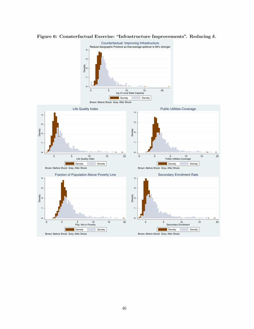
Figure 6: Counterfactual Exercise: “Infrastructure Improvements”. Reducing δ.
0.1
.2.3
.4D
ensi
ty
0 5 10 15 20log of Local State Capacity
Density Density
Brown: Before Shock Grey: After Shock
Reduce Geographic Frictions so that average spillover is 50% strongerCounterfactual: Improving Infrastructure
0.1
.2.3
.4D
ensi
ty
0 5 10 15 20Life Quality Index
Density Density
Brown: Before Shock Grey: After Shock
Life Quality Index
0.1
.2.3
.4D
ensi
ty
-5 0 5 10 15 20Public Utilities Coverage
Density Density
Brown: Before Shock Grey: After Shock
Public Utilities Coverage
0.1
.2.3
.4D
ensi
ty
-5 0 5 10 15 20Pop. Not in Poverty
Density Density
Brown: Before Shock Grey: After Shock
Fraction of Population Above Poverty Line
0.1
.2.3
.4D
ensi
ty
0 5 10 15 20Secondary Enrollment
Density Density
Brown: Before Shock Grey: After Shock
Secondary Enrollment Rate
46

Figure 7: Counterfactual Exercise: “Homogenizing National State Presence”
0.1
.2.3
.4D
ensi
ty
0 5 10 15 20 25log of Local State Capacity
Density Density
Brown: Before Shock Grey: After Shock
Take all municipalities below Median to the MedianCounterfactual: Homogenizing National State Presence
0.1
.2.3
.4D
ensi
ty
0 5 10 15 20Life Quality Index
Density Density
Brown: Before Shock Grey: After Shock
Life Quality Index
0.1
.2.3
.4D
ensi
ty
-5 0 5 10 15 20Public Utilities Coverage
Density Density
Brown: Before Shock Grey: After Shock
Public Utilities Coverage
0.1
.2.3
.4D
ensi
ty
-5 0 5 10 15 20Pop. Not in Poverty
Density Density
Brown: Before Shock Grey: After Shock
Fraction of Population Above Poverty Line
0.1
.2.3
.4D
ensi
ty
0 5 10 15 20Secondary Enrollment
Density Density
Brown: Before Shock Grey: After Shock
Secondary Enrollment Rate
47

Tables
!"#$%&'
!"#$"%&'( (%") (%*+") ,-")*".*&/%0+"-+1))*+"&,&'-'&./0"0'.12'3+$'( 45657 58688 58964:
)*+"&,&'-'&.;<3$+$="&$0>.?@=&*>''( AB64A 48688 B7:697
C"0$*3"&,&'-'&.;<3$+$="&$0>.?@=&*>''( 58:B6BB 448688 DA88644
)$E'.F<"&$0>.G3H'I 7A64B 7D698 5:68:
J<%&$+.K0$&$0$'(.L*-'#"2'.M"0' 9:6D5 9:6:N 45694
O#"+0$*3.*E.J*=<&"0$*3."%*-'.J*-'#0>.)$3' 9D657 9A6:: 5A678
/'+*3H"#>.?3#*&&@'30.M"0' 869B 869N 864N
J#$@"#>.?3#*&&@'30.M"0' 86AD 5688 868A
!"++$3"0$*3.L*-'#"2'.M"0' 8679 8677 865D
L*&*3$"&./0"0'.PEE$+$"&( 96NA 8688 5446BN
L*&*3$"&./0"0'.12'3+$'( 869D 8688 86BD
Q$(0"3+'.0*.M*>"&.M*"H(.RS@(6T 4N68D 5:6B: :76N4
C<@%'#.*E.C'$2U%*#( 967A 9688 56DA
V'*H'($+.Q$(0"3+'.0*.C'$2U%*#(.RS@(6T 75:697 :ND6NN 55:6:A
V'*H'($+.!"#$"%$&$0>.$3.?&'-"0$*3.0*.C'$2U%*#( 46DD 46DA 8678
Q$(0"3+'.0*.L<##'30.W$2UX">.RS@(6T :657 5694 N699
)*32$0<H' ,D76DN ,D76B4 567D
)"0$0<H' 96N4 9694 467:
/<#E"+'.1#'".R/Y6.S@(T NNA64B 4D:698 5749655
?&'-"0$*3.R;0(6T 548N6D5 54N9688 BAD6ND
1-'#"2'.133<"&.M"$3E"&&.R@@6T 5BA769A 5N:8698 58ND659
J*=<&"0$*3.R888T :D6:D 5:6B5 48867N
C<@%'#.*E.;<3$+$="&$0$'( 585A
/%23.+4-+0%&,-"-+2-+32
L*-"#$"0'(
C'0X*#Z.!"#$"%&'(
L*&*3$"&./0"0'.J#'('3+'
J#*(='#$0>
/0"0'.L"="+$0>
48

!"#$%&'
( ' ) * + , - . /(0&123&4567"38%&79&:9;"$&:9"<6 !"###
'0&=%5>?#9@6A&"B%@">%&<567"38%&79&:9;"$&:9"<6 #"$%& !"###
)0&=%5>?#9@6&9C&3%5>?#9@6A&<567"38%&79&:9;"$&:9"<6 #"#'( #")!( !"###
*0&123&D9$935"$&9CC585"$6 *#"#+( *#"#,$ *#"#', !"###
+0&=%5>?#9@6A&"B%@">%&89$935"$&9CC585"$6 *#"!') #"#&+ #"#)# *#"#)! !"###
,0&=%5>?#9@6&9C&3%5>?#9@6A&89$935"$&9CC585"$6 *#"#'' #"#)& #"#,$ *#"#)$ *#"#,# !"###
-0&123&D9$935"$&67"7%&">%385%6 *#"!&( *#"#&+ *#"#!, #"('( *#"##) *#"##$ !"###
.0&=%5>?#9@6A&"B%@">%&89$935"$&67"7%&">%385%6 *#"$#% #"$(# #"$%& *#"#(& #"'+# #"##% #"#$$ !"###
/0&=%5>?#9@6&9C&3%5>?#9@6A&89$935"$&67"7%&">%385%6 *#"!+& #"$'' #"&&' *#"#&) #"#&! #"'#% #"#,% #"$%+ !"###
E57?53F4%G"@7H%37&IG"75"$&D9@@%$"7593&9C&7?%&J5679@58"$&I7"7%&K@%6%38%&B"@5"#$%6
49

!"#$%&'
()")%&*"+",-).&/%"012%3&"04!"# !$# !%#&& !'# !(# !)#&&&*+, -. ,/012345406,789/06:;; *+, -. ,/012345406,789/06:;;
<=/54>/6;45>1?4@6ABB/C98
305-63057 DEDF( DED(' DEDG) DEDHH DED(F DED)$!DEDDH# !DED"H# !DED"%# !DEDD(# !DED"%# !DED""#
305-63*8$89-"$&0)")%&8::-,-"$05- 2DEDD" 2DEDDH 2DED"% DEDD" 2DEDDG 2DED"'!DEDD(# !DEDDG# !DEDD(# !DEDD)# !DEDDG# !DEDD)"#
305-63*8$89-"$&0)")%&";%9,-%05- 2DED$H 2DED'$ 2DED$' 2DED%$ 2DED'' 2DED$)!DED"D# !DED"%# !DED""# !DED"%# !DED"'# !DED"%#
305-63<-0)"9,%&)8&28."$&28"35- DED"D 2DEDD' DEDD) DEDD( 2DEDDG DEDD"!DEDDF# !DED"%# !DED"D# !DEDDF# !DED"$# !DED""#
I/1>JKL586LB6I/1>JKL58M6NL@L?14@6,949/6LBB1C14@8 2DED%) 2DEDG)!DED($# !DED)D#
I/1>JKL586LB6I/1>JKL58M6NL@L?14@6,949/64>/?C1/8 DE"GH DE$%(!DEDG(# !DEDF"#
I/1>JKL586LB6I/1>JKL58M6O1894?C/69L6N@L8/896PL74@6PL4Q 2DEDG$ 2DE""$!DED$G# !DED%)#
R15896894>/6P68ST45/QU DE$H% DE$H'*=/51Q/?91B1C491L?6V/89U6666666666666666V/89689491891C DE(H) DE%$"NJ12,ST45/Q!$#66666666666666666666666666666666W2=4@T/ DEG') DEH($:/L>543J1C6NL?95L@8 X/8 X/8 X/8 X/8 X/8 X/8O/34590/?96R1Y/Q6ABB/C98 X/8 X/8 X/8 X/8 X/8 X/8*K8/5=491L?8 FG( FG( F)% "D"G "D"G "DD%
PLKT896894?Q45Q6/55L5861?6345/?9J/818E6&VJ/65/3L59/Q6/891049/8645/6045>1?4@6/BB/C98&&6NL@T0?6!%#6186/891049/Q6486468789/069L>/9J/56Z19J6CL@T0?86!%#[6!)#[6!F#[64?Q6!"$#6LB6V4K@/6(&&&NL@T0?6!)#6186/891049/Q6486468789/069L>/9J/56Z19J6CL@T0?86!%#[6!)#[6!F#[64?Q6!"$#6LB6V4K@/6)
VJ/6=/C9L56LB6CL?95L@861?C@TQ/86@L?>19TQ/[6@4919TQ/[68T5B4C/645/4[6/@/=491L?[6541?B4@@[6QT0076BL56Q/34590/?96C43194@[6Q1894?C/69L6CT55/?965L4QE
&=8;&8:&>1?#%2&8:&/19-,-+"$-).&@?+$8.%%0&+,
*89)%?+82"2.&()")%&@A1-$-#2-1?&B%0)&C%0+890%&&=8;&8:&>1?#%2&8:&/19-,-+"$-).&()")%&D;%9,-%0&+,
@A1-$-#2-1?&B%0)&C%0+890%4&069&E&FGH6IJKF>FLJ0J69&M&;F,KN&M&OKPJ&M&Q<&M&R
S-20)&()";%&=-9%"2&/83%$4&F>FLJ0J69&E>TFLJ,KUH&M&OKUV&M&%
50

!"#$%&'
!"#"$%"$&'()*+),-"./0 .10 .2033 .40 .50 .6033 .70 .80 .9033 ./:0 .//0 ./1033;<= >? =@A&"B'CDD ;<= >? =@A&"B'CDD ;<= >? =@A&"B'CDD ;<= >? =@A&"B'CDD
EF#-)$)&G*@'?)*+),-"'.DHIC>JH<'EKKELM=0
()*+,(-*+ :N576 :N497 :N2/1 :N428 :N45: :N2/1 :N2:9 :N2/: :N2/1 :N2/9 :N181 :N2/1.:N:760 .:N/650 .:N:570 .:N:650 .:N/490 .:N:570 .:N:550 .:N/6/0 .:N:570 .:N:690 .:N1440 .:N:570
()*+,(-*. :N:2: :N:2/ :N:29 :N:25 :N:25 :N:24 :N:2/ :N:19 :N:19 :N:2: :N:4/ :N:2:.:N::40 .:N::60 .:N::70 .:N::40 .:N::50 .:N::50 .:N::40 .:N::50 .:N::50 .:N::60 .:N::70 .:N::50
K+*A&'=&)O"'<+$")*'DG%"-P'
Q)-%'&"A&'#R()-S"'TG*'UG+$&'A+O$+T+V)$V"'GT'+$A&*SB"$&A :N::: :N::: :N::: :N:::K+*A&'=&)O"'I'AWS)*"% :N514 :N514 :N514 :N514K+*A&'=&)O"'<+$")*'DG%"-P'
Q)-%'&"A&'#R()-S"'TG*'UG+$&'A+O$+T+V)$V"'GT'+$A&*SB"$&A :N::: :N::: :N::: :N:::K+*A&'=&)O"'I'AWS)*"% :N74/ :N74: :N74: :N724C"GO*)#X+V'LG$&*G-A Y"A Y"A Y"A Y"A Y"A Y"A Y"A Y"A Y"A Y"A Y"A Y"A!"#)*&B"$&'K+F"%'ETT"V&A Y"A Y"A Y"A Y"A Y"A Y"A Y"A Y"A Y"A Y"A Y"A Y"A;,A"*()&+G$A 972 972 962 975 975 962 975 975 962 965 965 962MX"'("V&G*'GT'VG$&*G-A'+$V-S%"A'-G$O+&S%"Z'-)&+&S%"Z'AS*T)V"')*")Z'"-"()&+G$Z'*)+$T)--Z'%SBB@'TG*'%"#)*&B"$&'V)#+&)-Z'%+A&)$V"'&G'VS**"$&'*G)%NIG,SA&'A&)$%)*%'"**G*A'+$'#)*"$&X"A+AN'3MX"'*"#G*&"%'"A&+B)&"A')*"'B)*O+$)-'"TT"V&A33LG-SB$A'.20Z'.60Z'.90Z')$%'./10')*"'UG+$&-@'"A&+B)&"%'[+&X'VG-SB$'.20'+$'M),-"'2\S,-+V']&+-+&+"A'VG("*)O"'+A'&X"')("*)O"'VG("*)O"'GT'HWS"%SV&Z'="[)O"Z')$%'E-"V&*+V+&@
/012-'^'/012334/'_'./01230`1341'_'/1.a03342'_'./1.a030`1344'_536'_'"
="VG$%'=&)O"'DG%"-P'#'^'b3A`1'_'c13/012-'_'534&_&78'_'d
A`1'^'/012334/'_'./01230`1341'_'/1.a03342'_'./1.a030`1344'_536'_'"
9:;-)%:+<=&">(&9?#$+3&@;;(-&A<:?3<?:"$&BC?"<+;>A<"<%&D")"3+<=&E%"-?:%(&"-F&&G;H&;I&/?J#%:&;I&E?>+3+)"$+<=&A<"<%&KH%>3+%-
<>KE'e]H<MY'>J!Ef'/998 \]g<>L']M><>M>E='L;?EIHCE':1 J;M'>J'\;?EIMY'1::5 =EL;J!HIY'EJI;<<DEJM'91R:1
51

!"#$%&'(
!"#"$%"$&'()*+),-"./0 .10 .2033 .40 .50 .6033 .70 .80 .9033 ./:0 .//0 ./1033;<= >? =@A&"B'CDD ;<= >? =@A&"B'CDD ;<= >? =@A&"B'CDD ;<= >? =@A&"B'CDD
EF#-)$)&G*@'?)*+),-"'.DHIC>JH<'EKKELM=0
)*+,-).+, :N2/9 :N1/5 :N/25 :N111 :N196 :N/25 :N/58 :N224 :N/25 :N/5/ :N:71 :N/25.:N:170 .:N/260 .:N:4:0 .:N:140 .:N/210 .:N:4:0 .:N:110 .:N/5/0 .:N:4:0 .:N:180 .:N/750 .:N:4:0
)*+,-).+/ :N:17 :N:18 :N:17 :N:17 :N:17 :N:18 :N:16 :N:1/ :N:12 :N:16 :N:21 :N:2:.:N::20 .:N::40 .:N::40 .:N::10 .:N::40 .:N::40 .:N::20 .:N::40 .:N::20 .:N::40 .:N::60 .:N::50
K+*A&'=&)O"'<+$")*'DG%"-P
Q)-%'&"A&'#R()-S"'TG*'UG+$&'A+O$+T+V)$V"'GT'+$A&*SB"$&A :N::/ :N::/ :N::/ :N:::K+*A&'=&)O"'I'AWS)*"% :N45: :N45: :N45: :N465K+*A&'=&)O"'<+$")*'DG%"-P'
Q)-%'&"A&'#R()-S"'TG*'UG+$&'A+O$+T+V)$V"'GT'+$A&*SB"$&A :N::: :N::: :N::: :N:::K+*A&'=&)O"'I'AWS)*"% :N7/6 :N7/5 :N7/5 :N7/9C"GO*)#X+V'LG$&*G-A Y"A Y"A Y"A Y"A Y"A Y"A Y"A Y"A Y"A Y"A Y"A Y"A!"#)*&B"$&'K+F"%'ETT"V&A Y"A Y"A Y"A Y"A Y"A Y"A Y"A Y"A Y"A Y"A Y"A Y"A;,A"*()&+G$A /:/4 /:/4 /::2 /:/7 /:/7 /::2 /:/7 /:/7 /::2 /::6 /::6 /::2MX"'("V&G*'GT'VG$&*G-A'+$V-S%"A'-G$O+&S%"Z'-)&+&S%"Z'AS*T)V"')*")Z'"-"()&+G$Z'*)+$T)--Z'%SBB@'TG*'%"#)*&B"$&'V)#+&)-Z'%+A&)$V"'&G'VS**"$&'*G)%NIG,SA&'A&)$%)*%'"**G*A'+$'#)*"$&X"A+AN'3MX"'*"#G*&"%'"A&+B)&"A')*"'B)*O+$)-'"TT"V&A33LG-SB$A'.20Z'.60Z'.90Z')$%'./10')*"'UG+$&-@'"A&+B)&"%'[+&X'VG-SB$'.60'+$'M),-"'2\S,-+V']&+-+&+"A'VG("*)O"'+A'&X"')("*)O"'VG("*)O"'GT'HWS"%SV&Z'="[)O"Z')$%'E-"V&*+V+&@
012.*%1,34&"5)&06#$,7&822).&93167361"$&:;6"3,2593"3%&<"*"7,34&=%".61%)&".>&&?2@&2A&B6C#%1&2A&=65,7,*"$,34&:C*$24%%.
="VG$%'=&)O"'DG%"-P'#'^'_3A`1'a'b13BDEF.'a'GHI&J&KL'a'c
'A`1'^'BDEF73I/'a'.BDEF70`13I1'a'B1.d073I2'a'.B1.d070`13I4'aG3M'a'"
BDEF.'^'BDEF73I/'a'.BDEF70`13I1'a'B1.d073I2'a'.B1.d070`13I4'aG3M'a'"
<>KE'e]H<MY'>J!Ef'/998 \]g<>L']M><>M>E='L;?EIHCE':1 J;M'>J'\;?EIMY'1::5 =EL;J!HIY'EJI;<<DEJM'91R:1
52

!"#$%&'(
!"#$% &# !"#$% &# !"#$% &# !"#$% &# !"#$% &#'( '( )* +,-(, +.-/, *'-0' +,-/ */-(( +0-)) 1/-/'
!"#$% &# !"#$% &# !"#$% &# !"#$% &# !"#$% &#'( //-+) )* 0.-(, +.-/, *1-0* +,-/ **-,. +0-)) ,'-01
23435%6474893:%$54;<"5=%4;%3>5%?<$@5"%#A%B#84B%;3435%4C5?895;
;3435%8474893:DE
;3435%8474893:DE
)*+%,-.%/01&!"2%&"$$&.3/-4-+"$-0-%5&6-07&50"0%&4"+"4-08&#%$96&.%:-"/&09&07%&.%:-"/;",0-"$&)<3-$-#,-3.&47"/=%&-/&.%:-"/&9>1
?%/%,"$&)<3-$-#,-3.&47"/=%&-/&.%:-"/&9>1
!"4839#?%=<5%3#%F9"583%GAA583E!"4839#?%=<5%3#%279BB#H5";E
I9A5%J<4B93:%K?=5L
0/-*M +,-0M 0.-*M +0-.M
I9A5%J<4B93:%K?=5L
NB399395;%6#H5"4C5 M%?#3%9?%O#H5"3: 258#?=4":%G?"#BB$5?3
.*-.M
NB399395;%6#H5"4C5 M%?#3%9?%O#H5"3: 258#?=4":%G?"#BB$5?3
)(-)M .0-.M ).-*M
53

!"#$%&'
!"#"$%"$&'()*+),-"./0 .10 .20 .30 .40 .50 .60 .7089: ;< 89: ;< 89: ;< 89: ;<
=>#-)$)&?*@'<)*+),-"'.ABCD;EB9'=FF=GH:0
()*+,(-*+ IJ521 IJ24I IJ4/1 IJ256 IJ243 IJ14I IJ242 IJ12I.IJI2K0 .IJ/150 .IJI240 .IJ/IK0 .IJI250 .IJ//50 .IJI4I0 .IJ/710
()*+,(-*. IJI13 IJI2I IJI2I IJI22 IJI16 IJI17 IJI15 IJI3I.IJI130 .IJII50 .IJII30 .IJII40 .IJII30 .IJII40 .IJII50 .IJII70
L)-%'&"M&'#N()-O"'P?*'Q?+$&'M+R$+P+S)$S"'?P'+$M&*OT"$&M IJIII IJIII IJIII IJIIIF+*M&':&)R"'C'MUO)*"% IJ116 IJ115 IJ115 IJ111
L)-%'&"M&'#N()-O"'P?*'Q?+$&'M+R$+P+S)$S"'?P'+$M&*OT"$&M IJIII IJIII IJIII IJIIIF+*M&':&)R"'C'MUO)*"% IJ63/ IJ63I IJ63I IJ623D"?R*)#V+S'G?$&*?-M W"M W"M W"M W"M W"M W"M W"M W"M!"#)*&T"$&'F+>"%'=PP"S&M W"M W"M W"M W"M W"M W"M W"M W"M8,M"*()&+?$M K62 K62 K64 K64 K64 K64 K54 K54
!"#"$%"$&'()*+),-".K0 ./I0 .//0 ./10 ./20 ./30 ./40 ./5089: ;< 89: ;< 89: ;< 89: ;<
=>#-)$)&?*@'<)*+),-"'.ABCD;EB9'=FF=GH:0
()*+,(-*+ IJ246 IJ/65 IJ15K IJ156 IJ/76 IJ112 IJ/57 IJIK4.IJI110 .IJIK10 .IJI1/0 .IJI740 .IJI1/0 .IJIK10 .IJI170 .IJ/120
()*+,(-*. IJI14 IJI16 IJI14 IJI14 IJI13 IJI11 IJI14 IJI2/.IJII20 .IJII30 .IJII10 .IJII30 .IJII20 .IJII30 .IJII30 .IJII50
L)-%'&"M&'#N()-O"'P?*'Q?+$&'M+R$+P+S)$S"'?P'+$M&*OT"$&M IJIII IJIII IJIII IJ171F+*M&':&)R"'C'MUO)*"% IJ162 IJ161 IJ161 IJIII
L)-%'&"M&'#N()-O"'P?*'Q?+$&'M+R$+P+S)$S"'?P'+$M&*OT"$&M IJIII IJIII IJIII IJIIIF+*M&':&)R"'C'MUO)*"% IJ6/5 IJ6/4 IJ6/4 IJ6/KD"?R*)#V+S'G?$&*?-M W"M W"M W"M W"M W"M W"M W"M W"M!"#)*&T"$&'F+>"%'=PP"S&M W"M W"M W"M W"M W"M W"M W"M W"M8,M"*()&+?$M /I/3 /I/3 /I/6 /I/6 /I/6 /I/6 /II5 /II5HV"'("S&?*'?P'S?$&*?-M'+$S-O%"M'-?$R+&O%"X'-)&+&O%"X'MO*P)S"')*")X'"-"()&+?$X'*)+$P)--X'%OTT@'P?*'%"#)*&T"$&'S)#+&)-X'%+M&)$S"'&?'SO**"$&'*?)%JC?,OM&'M&)$%)*%'"**?*M'+$'#)*"$&V"M+MJ'YHV"'*"#?*&"%'"M&+T)&"M')*"'T)*R+$)-'"PP"S&MZO,-+S'[&+-+&+"M'S?("*)R"'+M'&V"')("*)R"'S?("*)R"'?P'BUO"%OS&X':"\)R"X')$%'=-"S&*+S+&@
/01-)%0+23&"4(&/5#$+6&711(-&89":;%8&<=5"2+14>2"2%&?")"6+23&@%"-50%(&"-A&&B1C&1D&95E#%0&1D&@54+6+)"$+23&>2"2%&FC%46+%-
:"S?$%':&)R"'A?%"-]'#'^'_YM'`'a1Y9-'`'GYH'`'I!'`'b
9;F='c[B9HW';E!=d'/KK7 Z[e9;G'[H;9;H;=:'G8<=CBD='I1 E8H';E'Z8<=CHW'1II4 :=G8E!BCW'=EC899A=EH'K1NI1
>2"2%&?")"6+23&@%"-50%(&"-A&&B1C&1D&95E#%0&1D&@54+6+)"$+23&<E)$13%%-
F+*M&':&)R"'9+$")*'A?%"-]'M'^'96YH/'`'.960f1YH1'`'916YH2'`'.9160f1YH3'`GYJ'`'"
F+*M&':&)R"'9+$")*'A?%"-]'9-'^'96YH/'`'.960f1YH1'`'916YH2'`'.9160f1YH3'`GYJ'`'"
9;F='c[B9HW';E!=d'/KK7 Z[e9;G'[H;9;H;=:'G8<=CBD='I1 E8H';E'Z8<=CHW'1II4 :=G8E!BCW'=EC899A=EH'K1NI1
F+*M&':&)R"'9+$")*'A?%"-]'M'^'96YH/'`'.960f1YH1'`'916YH2'`'.9160f1YH3'`GYJ'`'"
F+*M&':&)R"'9+$")*'A?%"-]'9-'^'96YH/'`'.960f1YH1'`'916YH2'`'.9160f1YH3'`GYJ'`'"
:"S?$%':&)R"'A?%"-]'#'^'_YM'`'a1Y9-'`'GYH'`'I!'`'b
54

!"#$%&'
()")%&*"+",-).&/%"012%3&"04!"#"$%"$&'()*+),-"
./0 .10 .20 .30 .40 .50 ./60 .//0
789 :; 789 :; 789 :; 789 :;
<=#-)$)&>*?';)*+),-"'.@ABC:DA8'<EE<FG90
3+5-6305- H6I641 6I6JK H6I665 H6I/J1 H6I611 6I1/K 6I66/ 6I6/J
.6I6KL0 .6I1KK0 .6I6K40 .6I1/20 .6I61K0 .6I/540 .6I6110 .6I1610
3+5-63057 6I666 6I66J 6I662 6I66J 6I666 H6I66/ H6I661 6I666
.6I6630 .6I66J0 .6I6630 .6I66J0 .6I66K0 .6I6630 .6I66K0 .6I6630
M)-%'&"N&'#H()-O"'P>*'Q>+$&'N+R$+P+S)$S"'>P'+$N&*OT"$&N 6I666 6I666 6I666 6I66/
E+*N&'9&)R"'B'NUO)*"% 6I313 6I2J3 6I312 6I236
M)-%'&"N&'#H()-O"'P>*'Q>+$&'N+R$+P+S)$S"'>P'+$N&*OT"$&N 6I666 6I666 6I666 6I666
E+*N&'9&)R"'B'NUO)*"% 6I4K2 6I4/5 6I426 6I4/3
C">R*)#V+S'F>$&*>-N W"N W"N W"N W"N W"N W"N W"N W"N
!"#)*&T"$&'E+="%'<PP"S&N W"N W"N W"N W"N W"N W"N W"N W"N
7,N"*()&+>$N LJK LJK /662 /662 L43 L43 /6/4 /6/4
GV"'("S&>*'>P'S>$&*>-N'+$S-O%"N'->$R+&O%"X'-)&+&O%"X'NO*P)S"')*")X'"-"()&+>$X'*)+$P)--X'%OTT?'P>*'%"#)*&T"$&'S)#+&)-X'%+N&)$S"'&>'SO**"$&'*>)%I
B>,ON&'N&)$%)*%'"**>*N'+$'#)*"$&V"N+NI'
YGV"'*"#>*&"%'"N&+T)&"N')*"'T)*R+$)-'"PP"S&N
8$",%#9&:;%2,-0%4&<")-9="$$.&>%)%2/-=%3&8290+%2-).&"=3&81#$-,&?9930&@1),9/%0&()21,)12"$&:A1")-9=&B9C&9D&<1/#%2&9D&E1=-,-+"$-).&()")%&FC%=,-%0&+, &B9C&9D&<1/#%2&9D&E1=-,-+"$-).&:/+$9.%%0&+,
ZB:@ABW'<DB788@<DG'L1H61 ;AFF:DAG:7D'F7;<BAC<'/LL5 ZB:@ABW'<DB788@<DG'L1H61 ;AFF:DAG:7D'F7;<BAC<'/LL5
9"S>$%'9&)R"'@>%"-['#'\']YN^1'_'`1Y<GHI0'_;YJ'_'a!'_'b
E+*N&'9&)R"'8+$")*'@>%"-['N^1'\'<GHI,YJ/'_'.<GHI,0^1YJ1'_'<1.c0,YJK'_'.<1.c0,0^1YJ2'_;YK'_'"
E+*N&'9&)R"'8+$")*'@>%"-['<GHI0'\'<GHI,YJ/'_'.<GHI,0^1YJ1'_'<1.c0,YJK'_'.<1.c0,0^1YJ2'_;YK'_'"
55
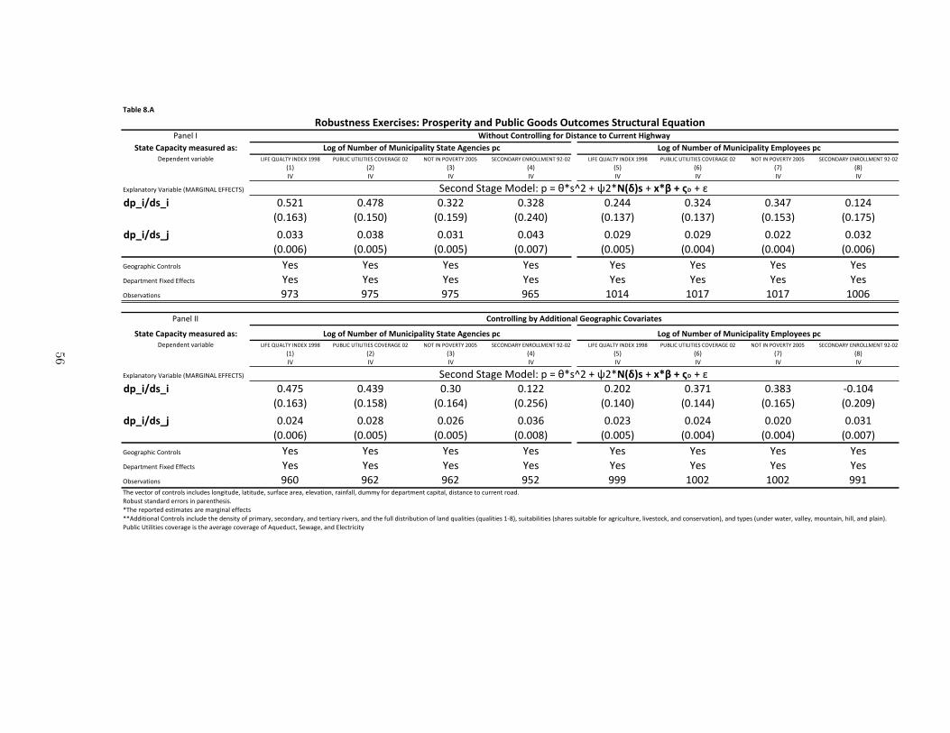
!"#$%&'()
!"#$%&'
*+"+%&,"-"./+0&1%"234%5&"26($)$#*$#+&,"-."/%$ 0'12&345067&'8(29&:;;< !4=0'>&46'0'6'2?&>@A2B5C2&DE 8@6&'8&!@A2B67&EDDF ?2>@8(5B7&28B@00G286&;EHDE 0'12&345067&'8(29&:;;< !4=0'>&46'0'6'2?&>@A2B5C2&DE 8@6&'8&!@A2B67&EDDF ?2>@8(5B7&28B@00G286&;EHDE
I:J IEJ IKJ ILJ IFJ IMJ INJ I<J
'A 'A 'A 'A 'A 'A 'A 'A
2O)%"#"+P-Q&A"-."/%$&IG5BC'850&2112>6?J
5-7/8527/ DRFE: DRLN< DRKEE DRKE< DRELL DRKEL DRKLN DR:EL
IDR:MKJ IDR:FDJ IDR:F;J IDRELDJ IDR:KNJ IDR:KNJ IDR:FKJ IDR:NFJ
5-7/85279 DRDKK DRDK< DRDK: DRDLK DRDE; DRDE; DRDEE DRDKE
IDRDDMJ IDRDDFJ IDRDDFJ IDRDDNJ IDRDDFJ IDRDDLJ IDRDDLJ IDRDDMJ
C$PS-")T.U&>P#+-P%V 7$V 7$V 7$V 7$V 7$V 7$V 7$V 7$V
($)"-+W$#+&1.O$*&2XX$U+V 7$V 7$V 7$V 7$V 7$V 7$V 7$V 7$V
@/V$-,"+.P#V ;NK ;NF ;NF ;MF :D:L :D:N :D:N :DDM
!"#$%&''
*+"+%&,"-"./+0&1%"234%5&"26($)$#*$#+&,"-."/%$ 0'12&345067&'8(29&:;;< !4=0'>&46'0'6'2?&>@A2B5C2&DE 8@6&'8&!@A2B67&EDDF ?2>@8(5B7&28B@00G286&;EHDE 0'12&345067&'8(29&:;;< !4=0'>&46'0'6'2?&>@A2B5C2&DE 8@6&'8&!@A2B67&EDDF ?2>@8(5B7&28B@00G286&;EHDE
I:J IEJ IKJ ILJ IFJ IMJ INJ I<J
'A 'A 'A 'A 'A 'A 'A 'A
2O)%"#"+P-Q&A"-."/%$&IG5BC'850&2112>6?J
5-7/8527/ DRLNF DRLK; DRKD DR:EE DREDE DRKN: DRK<K HDR:DL
IDR:MKJ IDR:F<J IDR:MLJ IDREFMJ IDR:LDJ IDR:LLJ IDR:MFJ IDRED;J
5-7/85279 DRDEL DRDE< DRDEM DRDKM DRDEK DRDEL DRDED DRDK:
IDRDDMJ IDRDDFJ IDRDDFJ IDRDD<J IDRDDFJ IDRDDLJ IDRDDLJ IDRDDNJ
C$PS-")T.U&>P#+-P%V 7$V 7$V 7$V 7$V 7$V 7$V 7$V 7$V
($)"-+W$#+&1.O$*&2XX$U+V 7$V 7$V 7$V 7$V 7$V 7$V 7$V 7$V
@/V$-,"+.P#V ;MD ;ME ;ME ;FE ;;; :DDE :DDE ;;:
6T$&,$U+P-&PX&UP#+-P%V&.#U%Y*$V&%P#S.+Y*$Z&%"+.+Y*$Z&VY-X"U$&"-$"Z&$%$,"+.P#Z&-".#X"%%Z&*YWWQ&XP-&*$)"-+W$#+&U").+"%Z&*.V+"#U$&+P&UY--$#+&-P"*R
BP/YV+&V+"#*"-*&$--P-V&.#&)"-$#+T$V.VR&
[6T$&-$)P-+$*&$V+.W"+$V&"-$&W"-S.#"%&$XX$U+V
[[5**.+.P#"%&>P#+-P%V&.#U%Y*$&+T$&*$#V.+Q&PX&)-.W"-QZ&V$UP#*"-QZ&"#*&+$-+."-Q&-.,$-VZ&"#*&+T$&XY%%&*.V+-./Y+.P#&PX&%"#*&\Y"%.+.$V&I\Y"%.+.$V&:H<JZ&VY.+"/.%.+.$V&IVT"-$V&VY.+"/%$&XP-&"S-.UY%+Y-$Z&%.,$V+PU]Z&"#*&UP#V$-,"+.P#JZ&"#*&+Q)$V&IY#*$-&^"+$-Z&,"%%$QZ&WPY#+".#Z&T.%%Z&"#*&)%".#JR&
!Y/%.U&4+.%.+.$V&UP,$-"S$&.V&+T$&",$-"S$&UP,$-"S$&PX&5\Y$*YU+Z&?$^"S$Z&"#*&2%$U+-.U.+Q
:;#32+<%22&=>%4./2%26&?4;2-%4/+0&"<5&?3#$/.&@;;52&A3+.;1%2&*+43.+34"$&=B3"+/;<
?$UP#*&?+"S$&GP*$%_&)&`&a[VbE&c&dE[CDEF2&c&>GH&I&JK&c&e
,;<+4;$$/<L�&)55/+/;<"$&@%;L4"-M/.&,;N"4/"+%2
?$UP#*&?+"S$&GP*$%_&)&`&a[VbE&c&dE[CDEF2&c&>GH&I&JK&c&e
&O;L&;P&C31#%4&;P&Q3</./-"$/+0&*+"+%&)L%<./%2&-. &O;L&;P&C31#%4&;P&Q3</./-"$/+0&=1-$;0%%2&-.R/+M;3+&,;<+4;$$/<L&P;4&K/2+"<.%&+;&,344%<+&S/LMT"0
&O;L&;P&C31#%4&;P&Q3</./-"$/+0&*+"+%&)L%<./%2&-. &O;L&;P&C31#%4&;P&Q3</./-"$/+0&=1-$;0%%2&-.
56

!"#$%&'()
!"#$%&'
*+"+%&,"-"./+0&1%"234%5&"26($)$#*$#+&,"-."/%$ 0'12&345067&'8(29&:;;< !4=0'>&46'0'6'2?&>@A2B5C2&DE 8@6&'8&!@A2B67&EDDF ?2>@8(5B7&28B@00G286&;EHDE 0'12&345067&'8(29&:;;< !4=0'>&46'0'6'2?&>@A2B5C2&DE 8@6&'8&!@A2B67&EDDF ?2>@8(5B7&28B@00G286&;EHDE
I:J IEJ IKJ ILJ IFJ IMJ INJ I<J
'A 'A 'A 'A 'A 'A 'A 'A
2O)%"#"+P-Q&A"-."/%$&IG5BC'850&2112>6?J
5-7/8527/ DRM<L DRFL; DRF:E DRLFN DRLFM DRKKN DRKFE DREEF
IDR:ELJ IDR::;J IDR:KEJ IDR:<;J IDRD<MJ IDRD<KJ IDRD;KJ IDR:EKJ
5-7/85279 DRDKL DRDLM DRDKL DRDLL DRDEM DRDKF DRDEM DRDKL
IDRDD<J IDRDDNJ IDRDDNJ IDRD:DJ IDRDDMJ IDRDDFJ IDRDDMJ IDRDD<J
C$PS-")T.U&>P#+-P%V 7$V 7$V 7$V 7$V 7$V 7$V 7$V 7$V
($)"-+W$#+&1.O$*&2XX$U+V 7$V 7$V 7$V 7$V 7$V 7$V 7$V 7$V
@/V$-,"+.P#V ;NK ;NF ;NF ;MF :D:L :D:N :D:N :DDM
!"#$%&''
*+"+%&,"-"./+0&1%"234%5&"26($)$#*$#+&,"-."/%$ 0'12&345067&'8(29&:;;< !4=0'>&46'0'6'2?&>@A2B5C2&DE 8@6&'8&!@A2B67&EDDF ?2>@8(5B7&28B@00G286&;EHDE 0'12&345067&'8(29&:;;< !4=0'>&46'0'6'2?&>@A2B5C2&DE 8@6&'8&!@A2B67&EDDF ?2>@8(5B7&28B@00G286&;EHDE
I:J IEJ IKJ ILJ IFJ IMJ INJ I<J
'A 'A 'A 'A 'A 'A 'A 'A
2O)%"#"+P-Q&A"-."/%$&IG5BC'850&2112>6?J
5-7/8527/ DRME; DRFM: DRLKD DRFDF DRKND DRK:F DRK:< DR:MF
IDR::MJ IDR:DNJ IDR::;J IDR:<DJ IDRDN<J IDRDNMJ IDRD<<J IDR:EDJ
5-7/85279 DRD:D DRD:E DRD:D DRD:K DRDD< DRD:D DRDD< DRD::
IDRDDEJ IDRDDEJ IDRDDEJ IDRDDKJ IDRDD:J IDRDD:J IDRDD:J IDRDDEJ
C$PS-")T.U&>P#+-P%V 7$V 7$V 7$V 7$V 7$V 7$V 7$V 7$V
($)"-+W$#+&1.O$*&2XX$U+V 7$V 7$V 7$V 7$V 7$V 7$V 7$V 7$V
@/V$-,"+.P#V ;NK ;NF ;NF ;MF :D:L :D:N :D:N :DDM
6T$&,$U+P-&PX&UP#+-P%V&.#U%Y*$V&%P#S.+Y*$Z&%"+.+Y*$Z&VY-X"U$&"-$"Z&$%$,"+.P#Z&-".#X"%%Z&*YWWQ&XP-&*$)"-+W$#+&U").+"%Z&*.V+"#U$&+P&UY--$#+&-P"*R
BP/YV+&V+"#*"-*&$--P-V&.#&)"-$#+T$V.VR&
[6T$&-$)P-+$*&$V+.W"+$V&"-$&W"-S.#"%&$XX$U+V
!Y/%.U&4+.%.+.$V&UP,$-"S$&.V&+T$&",$-"S$&UP,$-"S$&PX&5\Y$*YU+Z&?$]"S$Z&"#*&2%$U+-.U.+Q
:2/;<&;%/<=#>42&>?&;%/<=#>42&>?&;%/<=#>42&"2&/;2+431%;+2&@><&>?&A31#%4&>?&B3;/./-"$/+0&*+"+%&C<%;./%2&-. &@><&>?&A31#%4&>?&B3;/./-"$/+0&D1-$>0%%2&-.
E%?/;/;<&$/;F2&+>&/;.$35%&;%/<=#>42&";5&;%/<=#>42&>?&;%/<=#>42&@><&>?&A31#%4&>?&B3;/./-"$/+0&*+"+%&C<%;./%2&-. &@><&>?&A31#%4&>?&B3;/./-"$/+0&D1-$>0%%2&-.
?$UP#*&?+"S$&GP*$%^&)&_&`[VaE&b&cE[AGHI2&b&JKL&M&NE&b&d
O>#32+;%22&DJ%4./2%26&P4>2-%4/+0&";5&P3#$/.&Q>>52&R3+.>1%2&*+43.+34"$&DS3"+/>;
?$UP#*&?+"S$&GP*$%^&)&_&`[VaE&b&cE[AGHI2&b&JKL&M&NE&b&d
57

!"#$%&'()
!"#$%&'
*+"+%&)","-.+/&0%"123%4&"15($)$#*$#+&,"-."/%$ 0'12&345067&'8(29&:;;< !4=0'>&46'0'6'2?&>@A2B5C2&DE 8@6&'8&!@A2B67&EDDF ?2>@8(5B7&28B@00G286&;EHDE 0'12&345067&'8(29&:;;< !4=0'>&46'0'6'2?&>@A2B5C2&DE 8@6&'8&!@A2B67&EDDF ?2>@8(5B7&28B@00G286&;EHDE
I:J IEJ IKJ ILJ IFJ IMJ INJ I<J
'A 'A 'A 'A 'A 'A 'A 'A
2O)%"#"+P-Q&A"-."/%$&IG5BC'850&2112>6?J
4,6.7416. DRND: DRM<M DRK;E DRLL; DRKM; DRF:K DRL:F DR::F
IDR:NDJ IDR:FFJ IDR:M;J IDRELMJ IDR:L:J IDR:FDJ IDR:MFJ IDR:<NJ
4,6.74168 DRDEL DRDK: DRDKE DRDKN DRDEE DRDEK DRDEE DRDKD
IDRDDNJ IDRDDMJ IDRDDMJ IDRDD;J IDRDDFJ IDRDDFJ IDRDDFJ IDRDDNJ
C$PS-")T.U&>P#+-P%V 7$V 7$V 7$V 7$V 7$V 7$V 7$V 7$V
($)"-+W$#+&1.O$*&2XX$U+V 7$V 7$V 7$V 7$V 7$V 7$V 7$V 7$V
@/V$-,"+.P#V ;NK ;NF ;NF ;MF :D:L :D:N :D:N :DDM
!"#$%&''
*+"+%&)","-.+/&0%"123%4&"15($)$#*$#+&,"-."/%$ 0'12&345067&'8(29&:;;< !4=0'>&46'0'6'2?&>@A2B5C2&DE 8@6&'8&!@A2B67&EDDF ?2>@8(5B7&28B@00G286&;EHDE 0'12&345067&'8(29&:;;< !4=0'>&46'0'6'2?&>@A2B5C2&DE 8@6&'8&!@A2B67&EDDF ?2>@8(5B7&28B@00G286&;EHDE
I:J IEJ IKJ ILJ IFJ IMJ INJ I<J
'A 'A 'A 'A 'A 'A 'A 'A
2O)%"#"+P-Q&A"-."/%$&IG5BC'850&2112>6?J
4,6.7416. DRFDL DRLND DRKEM DRKD: DRLN< DRLMK DRK<; DRKLE
IDR:MMJ IDR:FDJ IDR:MKJ IDREFKJ IDR:NDJ IDR:N<J IDR:<LJ IDRELFJ
4,6.74168 DRDK: DRDKF DRDE; DRDL: DRDEL DRDEF DRDED DRDE<
IDRDDMJ IDRDDFJ IDRDDFJ IDRDDNJ IDRDDFJ IDRDDFJ IDRDDLJ IDRDDMJ
C$PS-")T.U&>P#+-P%V 7$V 7$V 7$V 7$V 7$V 7$V 7$V 7$V
($)"-+W$#+&1.O$*&2XX$U+V 7$V 7$V 7$V 7$V 7$V 7$V 7$V 7$V
@/V$-,"+.P#V ;NK ;NF ;NF ;MF :D:L :D:N :D:N :DDM
6T$&,$U+P-&PX&UP#+-P%V&.#U%Y*$V&%P#S.+Y*$Z&%"+.+Y*$Z&VY-X"U$&"-$"Z&$%$,"+.P#Z&-".#X"%%Z&*YWWQ&XP-&*$)"-+W$#+&U").+"%Z&*.V+"#U$&+P&UY--$#+&-P"*R
BP/YV+&V+"#*"-*&$--P-V&.#&)"-$#+T$V.VR&
[6T$&-$)P-+$*&$V+.W"+$V&"-$&W"-S.#"%&$XX$U+V
!Y/%.U&4+.%.+.$V&UP,$-"S$&.V&+T$&",$-"S$&UP,$-"S$&PX&5\Y$*YU+Z&?$]"S$Z&"#*&2%$U+-.U.+Q
&9:;&:<&=20#%3&:<&>2?.-.,"$.+/&*+"+%&@;%?-.%1&,- &9:;&:<&=20#%3&:<&>2?.-.,"$.+/&A0,$:/%%1&,-
?$UP#*&?+"S$&GP*$%^&)&_&`[VaE&b&cE[=BCD1&b&EFG&H&IJ&b&d
AE-$24.?;&J.1+"?-%&+:&K:/"$&K:"41&"1&L?1+320%?+1&9:;&:<&=20#%3&:<&>2?.-.,"$.+/&*+"+%&@;%?-.%1&,- &9:;&:<&=20#%3&:<&>2?.-.,"$.+/&A0,$:/%%1&,-
?$UP#*&?+"S$&GP*$%^&)&_&`[VaE&b&cE[=BCD1&b&EFG&H&IJ&b&d
AE-$24.?;&):$:?."$&A0,$:/%%1&"1&.?1+320%?+1
K:#21+?%11&AE%3-.1%15&M3:1,%3.+/&"?4&M2#$.-&N::41&O2+-:0%1&*+32-+23"$&AP2"+.:?
58

!"#$%&'
()")%&*"+",-).&/%"012%3&"04 &567&68&91/#%2&68&:1;-,-+"$-).&()")%&<7%;,-%0&+, &567&68&91/#%2&68&:1;-,-+"$-).&=/+$6.%%0&+,!"# !$#%& %&
'()*+,)-.+*,/0+1-233)456
30>-?30>@ 7879: 7879;!787"<# !787"=#
30>-?3*6$6;-"$&0)")%&688-,-"$0>- 7877; >7877"!7877?# !7877?#
30>-?3*6$6;-"$&0)")%&"7%;,-%0>- >787=: >787:"!787"$# !787":#
30>-?3A-0)";,%&)6&26."$&26"3>- >7877= >7877<!787""# !787"$#
@)A,*+BC/4-DA05*A16 E)6 E)6F)B+*5G)05-H/I)J-233)456 E)6 E)6KL6)*(+5/A06 M<9 "7"<
NALO65-65+0J+*J-)**A*6-/0-B+*)05C)6/68-PQC)-*)BA*5)J-)65/G+5)6-+*)-G+*,/0+1-)33)456
QC)-()45A*-A3-4A05*A16-/041OJ)6-1A0,/5OJ)R-1+5/5OJ)R-6O*3+4)-+*)+R-)1)(+5/A0R-*+/03+11R-JOGGS-3A*-J)B+*5G)05-4+B/5+1R-J/65+04)-5A-4O**)05-*A+J8
*6;)26$$-;7&862&9")-6;"$B$%C%$%"1,2",.*6;)%/+62"2.&()")%&=D1-$-#2-1/&E%0)&F%0+6;0%&
=D1-$-#2-1/&E%0)&F%0+6;0%4&0?;&G&HIJ?KLMH9HNL0L?;&O&7H,MP&O&QMRL&O&SA&O&T
59
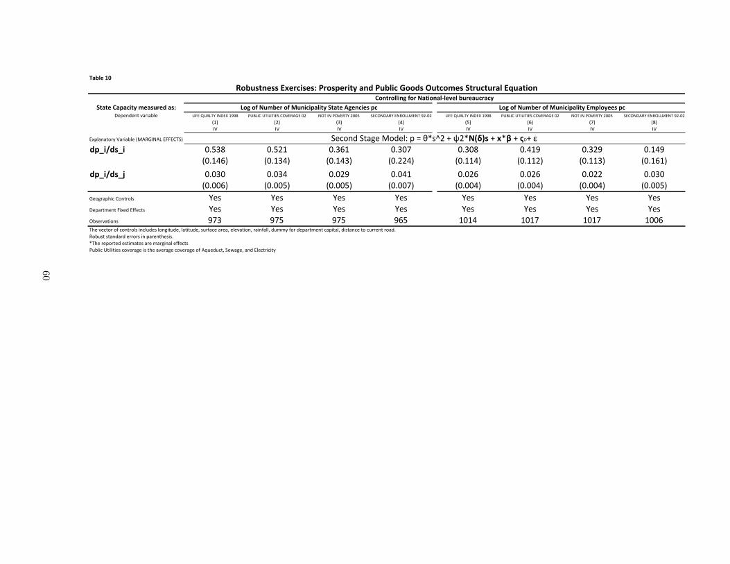
!"#$%&'(
)*"*%&+","-.*/&0%"123%4&"15!"#"$%"$&'()*+),-" ./01'234.56'/7!18'9::; <3=./>'35/./5/1?'>@A1B4C1'DE 7@5'/7'<@A1B56'EDDF ?1>@7!4B6'[email protected]':EHDE ./01'234.56'/7!18'9::; <3=./>'35/./5/1?'>@A1B4C1'DE 7@5'/7'<@A1B56'EDDF ?1>@7!4B6'[email protected]':EHDE
I9J IEJ IKJ ILJ IFJ IMJ INJ I;J
/A /A /A /A /A /A /A /A
1O#-)$)&P*Q'A)*+),-"'IG4BC/74.'1001>5?J
4,6.7416. DRFK; DRFE9 DRKM9 DRKDN DRKD; DRL9: DRKE: DR9L:
IDR9LMJ IDR9KLJ IDR9LKJ IDREELJ IDR99LJ IDR99EJ IDR99KJ IDR9M9J
4,6.74168 DRDKD DRDKL DRDE: DRDL9 DRDEM DRDEM DRDEE DRDKD
IDRDDMJ IDRDDFJ IDRDDFJ IDRDDNJ IDRDDLJ IDRDDLJ IDRDDLJ IDRDDFJ
C"PS*)#T+U'>P$&*P-V 6"V 6"V 6"V 6"V 6"V 6"V 6"V 6"V
!"#)*&W"$&'0+O"%'1XX"U&V 6"V 6"V 6"V 6"V 6"V 6"V 6"V 6"V
@,V"*()&+P$V :NK :NF :NF :MF 9D9L 9D9N 9D9N 9DDM
5T"'("U&P*'PX'UP$&*P-V'+$U-Y%"V'-P$S+&Y%"Z'-)&+&Y%"Z'VY*X)U"')*")Z'"-"()&+P$Z'*)+$X)--Z'%YWWQ'XP*'%"#)*&W"$&'U)#+&)-Z'%+V&)$U"'&P'UY**"$&'*P)%R
BP,YV&'V&)$%)*%'"**P*V'+$'#)*"$&T"V+VR'
[5T"'*"#P*&"%'"V&+W)&"V')*"'W)*S+$)-'"XX"U&V
<Y,-+U'3&+-+&+"V'UP("*)S"'+V'&T"')("*)S"'UP("*)S"'PX'4\Y"%YU&Z'?"])S"Z')$%'1-"U&*+U+&Q
?"UP$%'?&)S"'GP%"-^'#'_'`[VaE'b'cE[9:;<1'b'=[>'b'?!b'd
&@AB&AC&920#%3&AC&D2E.-.,"$.*/&)*"*%&FB%E-.%1&,- &@AB&AC&920#%3&AC&D2E.-.,"$.*/&G0,$A/%%1&,-
HA#21*E%11&G=%3-.1%15&I3A1,%3.*/&"E4&I2#$.-&JAA41&K2*-A0%1&)*32-*23"$&GL2"*.AE+AE*3A$$.EB&CA3&9"*.AE"$M$%N%$%"2-3"-/
60

!"#$%&''
!"#$%&'
()")%&*"+",-).&/%"012%3&"04($)$#*$#+&,"-."/%$ 0'12&345067&'8(29&:;;< !4=0'>&46'0'6'2?&>@A2B5C2&DE 8@6&'8&!@A2B67&EDDF ?2>@8(5B7&28B@00G286&;EHDE 0'12&345067&'8(29&:;;< !4=0'>&46'0'6'2?&>@A2B5C2&DE 8@6&'8&!@A2B67&EDDF ?2>@8(5B7&28B@00G286&;EHDE
I:J IEJ IKJ ILJ IFJ IMJ INJ I<J
'A 'A 'A 'A 'A 'A 'A 'A
2O)%"#"+P-Q&A"-."/%$&IG5BC'850&2112>6?J
3+5-6305- DRNFN DRN:N DRLK: DRF:E DRK<E DRL;D DRKL; DR:;M
IDR:M;J IDR:FLJ IDR:MMJ IDRENEJ IDR:L:J IDR:F<J IDR:FMJ IDREDFJ
3+5-63057 DRDE< DRDKE DRDEM DRDKL DRDEF DRDEL DRDED DRDEM
IDRDDMJ IDRDDMJ IDRDDFJ IDRDD<J IDRDDLJ IDRDDLJ IDRDDLJ IDRDDMJ
C$PS-")T.U&>P#+-P%V 7$V 7$V 7$V 7$V 7$V 7$V 7$V 7$V
($)"-+W$#+&1.O$*&2XX$U+V 7$V 7$V 7$V 7$V 7$V 7$V 7$V 7$V
@/V$-,"+.P#V N;; <D: <D: N;E <KK <KF <KF <EF
!"#$%&''
()")%&*"+",-).&/%"012%3&"04($)$#*$#+&,"-."/%$ 0'12&345067&'8(29&:;;< !4=0'>&46'0'6'2?&>@A2B5C2&DE 8@6&'8&!@A2B67&EDDF ?2>@8(5B7&28B@00G286&;EHDE 0'12&345067&'8(29&:;;< !4=0'>&46'0'6'2?&>@A2B5C2&DE 8@6&'8&!@A2B67&EDDF ?2>@8(5B7&28B@00G286&;EHDE
I:J IEJ IKJ ILJ IFJ IMJ INJ I<J
'A 'A 'A 'A 'A 'A 'A 'A
2O)%"#"+P-Q&A"-."/%$&IG5BC'850&2112>6?J
3+5-6305- :RDNE DR;FN DRKL; DR;:E DR<NM DR;LD DRLDD DRF:;
IDR:<NJ IDR:MDJ IDR:;:J IDRENDJ IDREENJ IDREFFJ IDR:<MJ IDREFKJ
3+5-63057 DRDEM DRDKE DRDEN DRDKE DRDE: DRDE: DRDED DRDEL
IDRDDNJ IDRDDMJ IDRDDMJ IDRD:DJ IDRDDMJ IDRDDMJ IDRDDFJ IDRDD<J
C$PS-")T.U&>P#+-P%V 7$V 7$V 7$V 7$V 7$V 7$V 7$V 7$V
($)"-+W$#+&1.O$*&2XX$U+V 7$V 7$V 7$V 7$V 7$V 7$V 7$V 7$V
@/V$-,"+.P#V N;; <D: <D: N;E <KK <KF <KF <EF
6T$&,$U+P-&PX&UP#+-P%V&.#U%Y*$V&%P#S.+Y*$Z&%"+.+Y*$Z&VY-X"U$&"-$"Z&$%$,"+.P#Z&-".#X"%%Z&*YWWQ&XP-&*$)"-+W$#+&U").+"%Z&*.V+"#U$&+P&UY--$#+&-P"*R
BP/YV+&V+"#*"-*&$--P-V&.#&)"-$#+T$V.VR&
[6T$&-$)P-+$*&$V+.W"+$V&"-$&W"-S.#"%&$XX$U+V
[[5**.+.P#"%&>P#+-P%V&.#U%Y*$&+T$&*$#V.+Q&PX&)-.W"-QZ&V$UP#*"-QZ&"#*&+$-+."-Q&-.,$-VZ&"#*&+T$&XY%%&*.V+-./Y+.P#&PX&%"#*&\Y"%.+.$V&I\Y"%.+.$V&:H<JZ&VY.+"/.%.+.$V&IVT"-$V&VY.+"/%$&XP-&"S-.UY%+Y-$Z&%.,$V+PU]Z&"#*&UP#V$-,"+.P#JZ&"#*&+Q)$V&IY#*$-&^"+$-Z&,"%%$QZ&WPY#+".#Z&T.%%Z&"#*&)%".#JR&
!Y/%.U&4+.%.+.$V&UP,$-"S$&.V&+T$&",$-"S$&UP,$-"S$&PX&5\Y$*YU+Z&?$^"S$Z&"#*&2%$U+-.U.+Q
A.P%$#U$&.V&W$"VY-$*&/Q&+T$&#YW/$-&PX&!"-"W.%.+"-Q&P-&CY$--.%%"&"++"U]V&P,$-&+T$&)$-.P*&:;;<HEDDLR
89,$13-:;&<2=/&)>%&:%)?=2@&/1:-,-+"$-)-%0&-:&)>%&AB)>&+%2,%:)-$%&=<&C-=$%:,%&D=;&=<&E1/#%2&=<&F1:-,-+"$-).&()")%&G;%:,-%0&+, &D=;&=<&E1/#%2&=<&F1:-,-+"$-).&8/+$=.%%0&+,
?$UP#*&?+"S$&GP*$%_&)&`&a[VbE&c&dE[EHIJ0&c&9KL&M&NO&c&e
P=#10):%00&89%2,-0%04&Q2=0+%2-).&":3&Q1#$-,&R==30&S1),=/%0&()21,)12"$&8T1")-=:89,$13-:;&<2=/&)>%&%0)-/")-:;&0"/+$%&/1:-,-+"$-)-%0&-:&)>%&AB)>&+%2,%:)-$%&=<&C-=$%:,%
&D=;&=<&E1/#%2&=<&F1:-,-+"$-).&()")%&G;%:,-%0&+, &D=;&=<&E1/#%2&=<&F1:-,-+"$-).&8/+$=.%%0&+,
?$UP#*&?+"S$&GP*$%_&)&`&a[VbE&c&dE[EHIJ0&c&9KL&M&NO&c&e
61

!"#$%&'(
)*+"$&,-"-%&."/"+0-1&2%"345%6&"3&)*7&*89 &24:0+0/"$0-1&,-"-%&;7%:+0%3&/+ 24:0+0/"$0-1&<=/$*1%%3&/+
>?' @A(B@ @A@BC
D@A@'EF D@A@''F
>?(&D)08%&G4"$0-1&H:6%IF @AJ'K 'A@E(
D@A'LKF D@AKC(F
>?(&DM4#$0+&N-0$0-0%3F 'A@@@ @AEJ@
D@A((OF D@A'JLF
>?(&DP*-&0:&M*Q%5-1F 'A(KO 'A'@@
D@AKEEF D@ACEJF
>?(&D,%+*:6"51&<:5*$$=%:-F 'A@B' 'A@J'
D@ACC(F D@A(''F
R @ALBB @ALBE
D@A@OLF D@A'@KF
STU?0V @A'BB @A(KL
D@A@'BFW D@A@KCFW
X @AL(K @AL'B
D@A(OEF D@A(BEF
Y 'AO'L 'AOCL
D@AKK(F D@AC'CF
Z"=%&[0-\&M5%6%-%5=0:%6&P"-0*:"$&)%Q%$&,-"-%&."/"+0-1.*:60-0*:"$&2)<
,-4+-45"$&M"5"=%-%5&<3-0="-%3
!"#$%&'()*+# OBK '@@K,-('+.'%./0$&)'()*+
Appendix
Proof of Proposition 1:
The second order condition for the municipality’s problem in equation (3) can be expressed
as
α [(κi + ξi)ni + ψ1Ni(δ)s]1
σ
1
li
[sili
] 1σ
{α
1
lisi
[sili
] 1σ
− 1
}− θ < 0
62
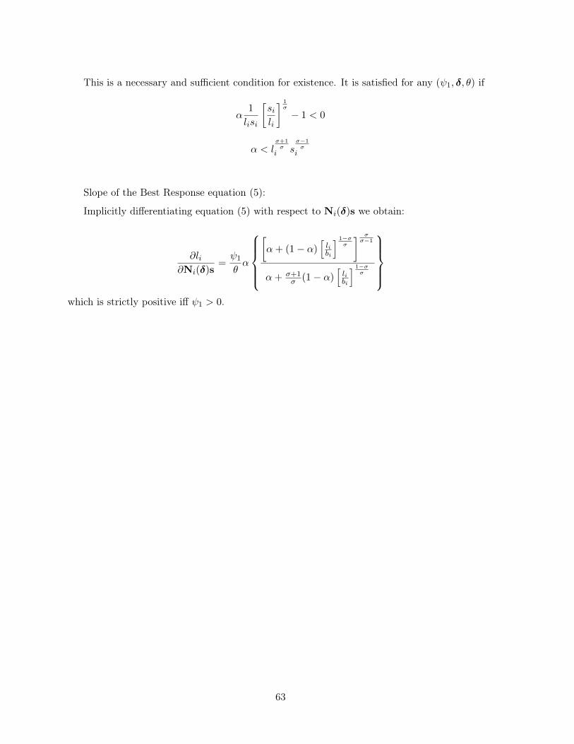
This is a necessary and sufficient condition for existence. It is satisfied for any (ψ1, δ, θ) if
α1
lisi
[sili
] 1σ
− 1 < 0
α < lσ+1σ
i sσ−1σ
i
Slope of the Best Response equation (5):
Implicitly differentiating equation (5) with respect to Ni(δ)s we obtain:
∂li∂Ni(δ)s
=ψ1
θα
[α+ (1− α)
[libi
] 1−σσ
] σσ−1
α+ σ+1σ (1− α)
[libi
] 1−σσ
which is strictly positive iff ψ1 > 0.
63


