
Statistical Health Grade System against Mechanical failures of
Power Transformers
Chao Hu1, Pingfeng Wang
2, Byeng D. Youn
3,*, Wook-Ryun Lee
4 and Joung Taek Yoon
3
1University of Maryland at College Park, Maryland, 20742, United States (Currently at Medtronic, Inc.)
2Wichita State University, Wichita, Kansas, 67260, United States
3Seoul National University, Seoul, 151-742, Korea
4Korea Electric Power Research Institute, Daejeon, 305-760, Korea
ABSTRACT
A health grade system against mechanical faults of power
transformers has been little investigated compared to those
for chemical and electrical faults. This paper thus presents a
statistical health grade system against mechanical faults in
power transformers used in nuclear power plant sites where
the mechanical joints and/or parts are the ones used for
constraining transformer cores. Two health metrics—root
mean square (RMS) and root mean square deviation (RMSD)
of spectral responses at harmonic frequencies—are first
defined using vibration signals acquired via in-site sensors
on fifty-four power transformers in several nuclear power
plants in sixteen months. We then investigate a novel
multivariate statistical model, namely copula, to statistically
model the populated data of the health metrics. The
preliminary study shows that the proposed health metrics
and statistical health grade system are feasible to monitor
and predict the health condition of the mechanical faults in
the power transformers.
1. INTRODUCTION
Power transformer is one of the most critical power
elements in nuclear power plants and an unexpected
transformer breakdown could cause a complete plant shut-
down with substantial societal expenses. It is very important
to ensure high reliability and maintainability of the
transformer during its operation. Investigations of the fault
causes have revealed that mechanical and electric faults are
primarily responsible for unexpected breakdowns of the
transformers (Lee et al., 2005). In total, 32 breakdowns of
main power transformers in Korean nuclear power plants
have been reported since 1978. Table 1 classifies these
breakdown causes into three groups (electrical, chemical,
and mechanical problems) and ways to manage them.
Preventive health management for power transformers has
been developed and implemented mainly for chemical and
electrical faults. Although mechanical failures are
responsible for about 40% of the transformer breakdowns,
the non-existence of generic health metrics or a health grade
system makes it difficult to perform preventive maintenance
actions for mechanical faults in a timely manner and only
corrective maintenance has been employed.
In the literature, substantial research has been carried out for
the health monitoring and diagnosis of power transformers.
An extensive review of health monitoring and diagnosis
methods of power transformers was provided in (Wang et
al., 2002) with a focus on all types of transformer failure
causes, and in (Pradhan, 2006; Saha, 2003) with a focus on
Insulation deterioration. Techniques commonly used for
health monitoring of power transformers can be summarized
as: (1) online partial discharge (PD) analysis (McArthur et
al., 2004), (2) dissolved gas analysis (DGA) (IEEE std.,
2008), (3) frequency response analysis (FRA) (Dick &
Erven, 1978), (4) moisture-in-oil analysis (Garcia et al.,
2005), (5) oil temperature analysis (Lee et al., 2005; Tang et
al., 2004), (6) winding temperature analysis (Picanço et al.,
2010), (7) load current and voltage analysis (Muhamad &
_____________________
* Corresponding author. † Chao Hu et al. This is an open-access article distributed under the terms of
the Creative Commons Attribution 3.0 United States License, which permits unrestricted use, distribution, and reproduction in any medium,
provided the original author and source are credited.
Annual Conference of Prognostics and Health Management Society 2012
2
Ali, 2006), and (8) online power factor analysis (Gong et al.,
2007). We note that the usage of the vibration signals in
monitoring the transformer health has been quite limited.
The transformer vibration generated by the core and
windings propagates through the transformer oil to the
transformer walls where vibration sensors can be placed for
vibration measurements. Bartoletti et al. (2004) transformed
measured acoustic and vibration signals into a frequency
domain and suggested a few metrics that could represent the
health status of transformers. Ji et al. (2006) acquired the
fundamental frequency component of the core vibration
signal as essential features to monitor and assess the
transformer health condition. García et al. (2006) proposed a
tank vibration model to detect the winding deformations in
power transformers and conducted the experimental
verification of the proposed model under different operating
conditions and in the presence of winding deformation .
Once sensory data are acquired through the health
monitoring, the data must be carefully analyzed for health
diagnosis in order to identify and classify failures modes.
Artificial intelligence (AI) techniques for pattern
recognition have been prevailing for this purpose. Among a
wide variety of AI techniques, ANNs have been most
widely used in the research dealing with transformer health
diagnosis (Huang, 2003; Hao & Cai-xin, 2007). Despite the
good accuracy reported in the literature, the use of ANNs is
limited by the intrinsic shortcomings including the danger of
over-fitting, the need for a large quantity of training data
and the numerical instability. In addition to ANNs, the fuzzy
logic (Hong-Tzer & Chiung-Cho, 1999; Su et al., 2000) and
expert systems (Purkait & Chakravorti, 2002; Saha &
Purkait, 2004) were also developed for transformer health
diagnosis. These two approaches take advantage of human
expertise to enhance the reliability and effectiveness of
health diagnosis systems. Recently, the support vector
machine (SVM) has been receiving growing attention with
remarkable diagnosis results (Fei et al., 2009; Fei & Zhang,
2009). The SVM, which employs the structural risk
minimization principle, achieves better generalization
performance than ANNs employing the traditional empirical
risk minimization principle, especially in cases of a small
quantity of training data (Shin & Cho, 2006).
The status of research on prognostics and health
management (PHM) of a power transformer can be
summarized as:
(1) Most health monitoring works for power transformers
are focused on chemical and electrical failures, but very
little on mechanical failures;
(2) Power transformer oil, gas and temperatures have been
widely used for health monitoring and diagnosis of
power transformers. In contrast, the vibration signal has
seldom been used for PHM in power transformer
applications;
(3) The PHM studies for power transformers currently stay
at the level of monitoring and diagnosis only, with few
works on the health prognostics and remaining useful
life (RUL) prediction.
This summary suggests the need to construct a health
management database, to formulate a health grade system
against mechanical faults, and to investigate the health
prognostics for power transformers. To this end, this study
presents a copula-based statistical health grade system
against mechanical faults of power transformers. The rest of
this paper is organized as follows: Section 2 introduces the
collection and pre-processing of the vibration data for power
transformer health monitoring; Section 3 presents the
developed copula based statistical health grade system for
power transformer health monitoring and prognostics
against mechanical faults followed by the conclusion in
Section 4.
2. DATA ACQUISITION AND PRE-PROCESSING
Failures of mechanical joints and/or other parts of power
transformers can be detected by analyzing mechanical
vibration properly. This section discusses the fundamentals
of transformer vibration, measurement procedures, and data
pre-processing.
Details (Occurrence) Occurrence Health
Analysis
Electrical
failures
- Natural disasters (1)
- Winding burnouts (2)
- Operator mistakes (2)
- Accidents in electric
power transmission (1) - Mal-operation (4)
- Product defects (1)
- Manufacturing defect (1)
- Product aging (1)
13 Insulation
Diagnosis Test
Chemical
failures
- Oil burnouts (1)
- Impurities in winding (1)
- Product defects (1)
- Increase of combustible gas
(3)
6 Insulating
Oil Analysis
Mechanical
failures
- Design defect (1)
- Manufacturing defect (1)
- Part corrosion (3)
- Joint failure (3)
- Crack, wear failure (5)
13 N.A.
Table 1. Breakdown Classification of Main Power
Transformers in Korean Nuclear Power Plants from 1978 to
2002

Annual Conference of Prognostics and Health Management Society 2012
3
2.1. Fundamentals of Transformer Vibration
Power transformer vibrations are primarily generated by the
magnetostriction and electrodynamic forces acting on the
core and windings during the operation. The vibration of the
core and windings propagates through the transformer oil to
the transformer walls where vibration sensors can be placed
for vibration measurements. The sensors cannot be placed
onto the joints because of the transformer oil and magnetic
and electric fields that can distort sensory signals. This
subsection gives a brief review of the fundamental physics
explaining vibrations in the transformer. Various vibration
sources exist inside a transformer, contributing to the tank
vibration. The transformer vibration mainly consists of the
core vibration originating from magnetostriction and the
winding vibration caused by electrodynamic forces resulting
from the interaction of the current in a winding with leakage
flux (García et al., 2006). Other vibration sources include
the characteristic acoustic wave produced by the tap changer
and periodic vibrations generated by the elements of the
cooling system (i.e., oil pumps and fans).
Alternating current (AC) with a constant frequency in power
transformers forms a magnetic field in the transformer core.
The magnetic field changes the shape of ferromagnetic
materials and produces mechanical vibration in the
transformer. This phenomenon is called “magnetostriction.”
As shown in Fig. 1, one cycle of the AC yields two peaks in
the magnetic field. Assume that an AC source with the
amplitude U0 and frequency f is applied to the drive and that
the amplitude is less than or just sufficient to saturate the
core. Then, the core vibration acceleration caused by
magnetostriction can be expressed as (Ji et al., 2006)
2 2
0 cos 4Ca U ft
(1)
We can observe from the above equation that the magnitude
of core vibration exhibits a linear relationship with the
square of the AC amplitude. Furthermore, the fundamental
frequency of the core vibration is twice that of the AC
frequency, as we can also observe in Fig. 1.
Winding vibrations are caused by electrodynamic forces
resulting from the interaction of the current in a winding
with leakage flux (Ji et al., 2006). These forces FW are
proportional to the square of the load current I, expressed as
2
WF I
(2)
Since the electromagnetic forces FW are proportional to the
vibration acceleration aW of the windings we then conclude
that (García et al., 2006)
2
Wa I
(3)
Thus, similar to the case of core vibration, the fundamental
frequency of winding vibrations is also twice the AC
frequency. The difference between these two types of
vibrations is that the magnitude of core vibration relies on
the voltage applied to the primary windings and is not
affected by the load current, while the magnitude of winding
vibrations is proportional to the square of the loading
current. In addition to the variables (voltage and current)
causing transformer vibration, the other factors (i.e.,
temperature, power factor) also have an influence on
vibration (Bartoletti et al., 2004), but due to the relatively
small influence, these factors are not considered in this
study. In fact, since power transformers in nuclear power
plants always operate at 100% full power, the variables
(voltage and current) and the power factor generally exhibit
very small variations over time. And since cooling systems
can effectively keep transformers cores and windings at
suitably low temperatures, the temperature factor also has
very small fluctuation.
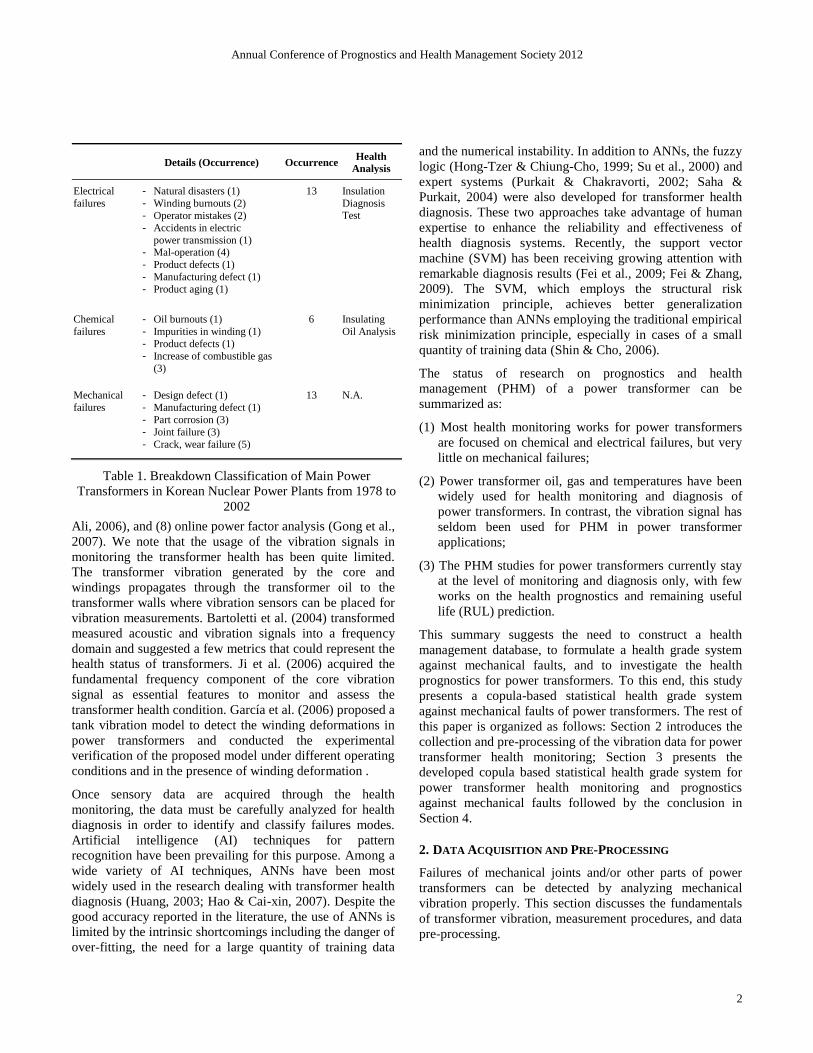
2.2. Vibration Signal Acquisition
In this study, fifty-four in-service power transformers in
four nuclear power plants were employed for acquiring
vibration signals. Among these transformers, three are
triple-phase transformers and the others are single-phase
transformers (see Table A in Appendix). These fifty-four
transformers have a wide range of ages, from less than one
year to about twenty-two years. This study employed B&K
4381 and PCB 357B33 accelerometers, which are charge
types with charge amplifiers (RION UV-06A). Depending
on the transformer size, 36 to162 accelerometers were used
to acquire the vibration signals from the transformers. The
sensors were evenly positioned within 1m on the single-
phase and triple-phase main transformers, as respectively
shown in Figs. 2(a) and (b). Measurements were conducted
along two directions (X and Y) on the surface of the
transformer frame and one perpendicular direction (Z) to the
surface. The accelerometers were installed on the flat
surface with a magnet base in order for easy measurement.
Figure 1. Magnetostriction in the transformer
Annual Conference of Prognostics and Health Management Society 2012
4
All measurements were obtained in the form of time-domain
signals in a full-power operation state of the power
transformers. In the state, all other subsidiary units affecting
vibration under normal operating conditions, such as forced
cooling systems and hydraulic pumps, were turned on. The
subsidiary units were supplied with 480 V AC power. In
most cases, the transformers convert primary electrical
values, i.e. voltages 22 kV and currents about 32 kA, to
proportional secondary values, i.e. voltages 345 kV and
current about 2 kA. The measurement system was powered
by an independent battery power system. Vibration velocity
[mm/sec] was measured at every 1.25 Hz in the frequency
range of 0-2000 Hz. The rated voltage always has a
frequency of 60 Hz. It is desirable to avoid taking the
measurement immediately after turning the transformer on
because the initial operation state of the transformer causes
transient vibration signals. It is certainly important to
acquire better sensory data and thus improve the
performance of power transformer health diagnostic by
optimizing the number of measure points and the allocation
of the sensors. For the study regarding the sensor network
optimization, readers are advised to the reference (Wang et
al., 2010).
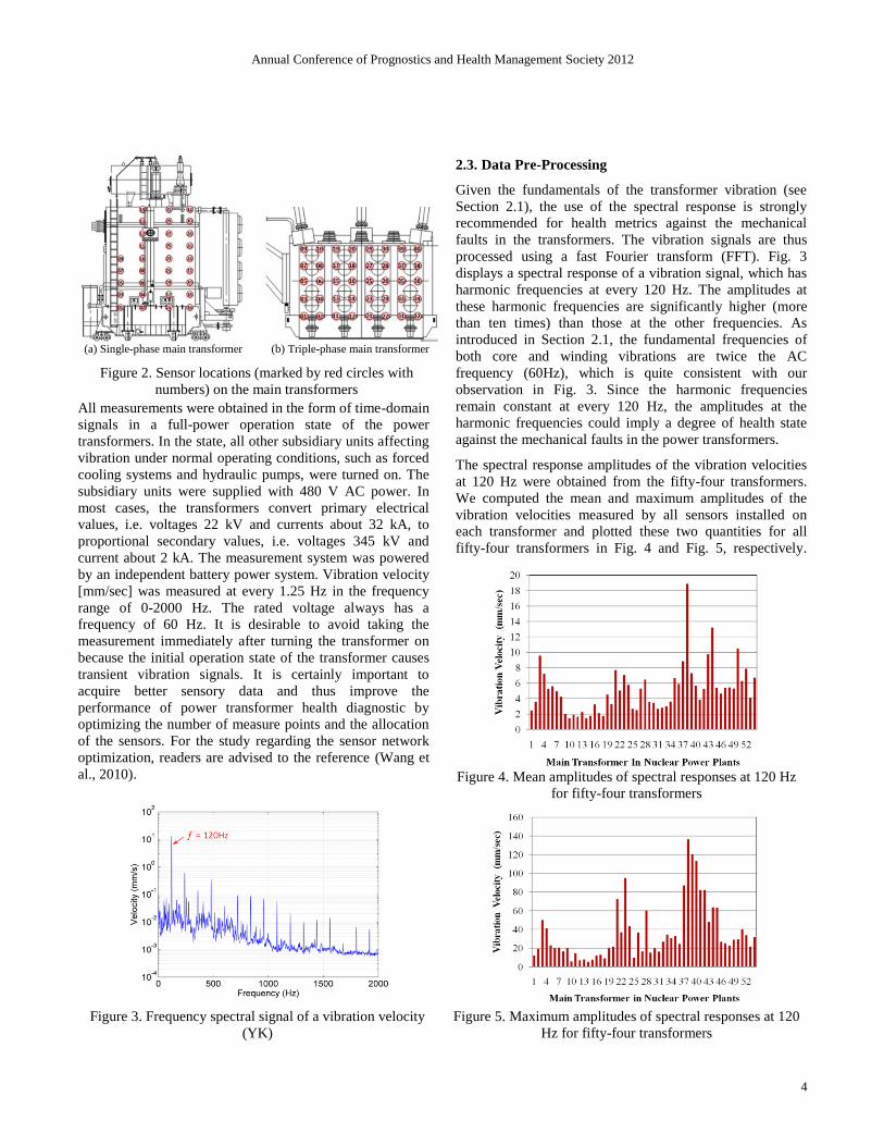
2.3. Data Pre-Processing
Given the fundamentals of the transformer vibration (see
Section 2.1), the use of the spectral response is strongly
recommended for health metrics against the mechanical
faults in the transformers. The vibration signals are thus
processed using a fast Fourier transform (FFT). Fig. 3
displays a spectral response of a vibration signal, which has
harmonic frequencies at every 120 Hz. The amplitudes at
these harmonic frequencies are significantly higher (more
than ten times) than those at the other frequencies. As
introduced in Section 2.1, the fundamental frequencies of
both core and winding vibrations are twice the AC
frequency (60Hz), which is quite consistent with our
observation in Fig. 3. Since the harmonic frequencies
remain constant at every 120 Hz, the amplitudes at the
harmonic frequencies could imply a degree of health state
against the mechanical faults in the power transformers.
The spectral response amplitudes of the vibration velocities
at 120 Hz were obtained from the fifty-four transformers.
We computed the mean and maximum amplitudes of the
vibration velocities measured by all sensors installed on
each transformer and plotted these two quantities for all
fifty-four transformers in Fig. 4 and Fig. 5, respectively.
(a) Single-phase main transformer (b) Triple-phase main transformer
Figure 2. Sensor locations (marked by red circles with
numbers) on the main transformers
Figure 3. Frequency spectral signal of a vibration velocity
(YK)
Figure 4. Mean amplitudes of spectral responses at 120 Hz
for fifty-four transformers
Figure 5. Maximum amplitudes of spectral responses at 120
Hz for fifty-four transformers
Annual Conference of Prognostics and Health Management Society 2012
5
Two observations can be made from the two figures. Firstly,
both quantities exhibit large variations among different
transformers. Specifically, the mean amplitudes of the
vibration velocities have a wide range of variation from 1.43
mm/sec to 18.87 mm/sec and the maximum amplitudes from
5.8 mm/sec to 136.43 mm/sec. It is believed that the aging
effect of the transformers and local resonance of the
transformer frame primarily causes the variation in the mean
and maximum amplitudes. Secondly, the maximum velocity
amplitude of each transformer is in general far greater than
the mean velocity amplitude of that transformer. This
observation can be attributed to the fact that, among more
than forty measurement points selected for each transformer,
two or three points at the upper part (closer to the top) of the
transformer wall typically gave much larger velocities than
the others.
3. HEALTH METRICS AND GRADE SYSTEM
This section presents the copula-based statistical health
grade system against mechanical faults of power
transformers.
3.1. Health Metrics
The frequency spectral signals from multiple sensors are
employed to monitor the health condition of the power
transformers. Two scalar health metrics are proposed in this
study: (1) root mean square (RMS) and (2) root mean square
deviation (RMSD). Their definitions and physical meanings
are given as follows:
RMS – The RMS is the quadratic measure of the vibration
mean velocities measured at every 2.5 Hz in the frequency
range of 2.5-2000 Hz. The RMS metric can be defined as
1 22000Hz
2
2.5Hz
, 1, ,54i f
f
RMS i
(4)
where f is the mean of the vibration velocity measured
from all sensors at a frequency f. It is generally known that
measured vibration velocities in the transformers become
greater as their health state degrades over years. This metric
is thus a useful health metric for transformer health
monitoring. However, the magnitudes of the mean velocity
also vary depending on the operating condition, the
transformer capacity and manufacturer. The RMS metric
may fail to classify a health condition of different
transformers experiencing mechanical degradation. This
underscores the need of another health monitoring metric.
RMSD – The RMSD is the quadratic measure of the
vibration deviation velocities measured at every 2.5 Hz in
the frequency range of 2.5-2000 Hz. The RMSD metric can
be defined as
1 22000Hz
2
2.5Hz
, 1, ,54i f
f
RMSD i
(5)
where f is the standard deviation of the vibration velocity
measured from all sensors at a frequency f. The same mean
velocities could indicate different health conditions if the
vibration measurements come from different transformers
under random operating conditions. The undesirable
situation above can be avoided by using both the RMS and
RMSD since the randomness in operating conditions and the
difference in transformers could affect the deviation of the
vibration velocity.
In cases where we have mechanical defects (for example,
winding deformations or loosened clamps in the core), the
magnitudes of winding or core vibration typically increase
because, as aged, electrodynamic forces (for winding)
generally grow; mechanical constraints (for core) loosen,
and structural strength becomes weaker. Moreover, the
winding or core vibration typically becomes more stochastic
and, to some degree, has variation over different transformer
samples. For the very reason, the magnitude (mean) and
randomness (standard deviation) of tank vibration amplitude
increase. The RMS and RMSD measures are capable of
capturing the transformer health degradation and its
variation. For the power transformers we investigated (i.e.,
step-up transformers used in power plants), the mean and
deviation of the vibration velocity at 120 Hz was generally
observed to become higher as transformers get older.
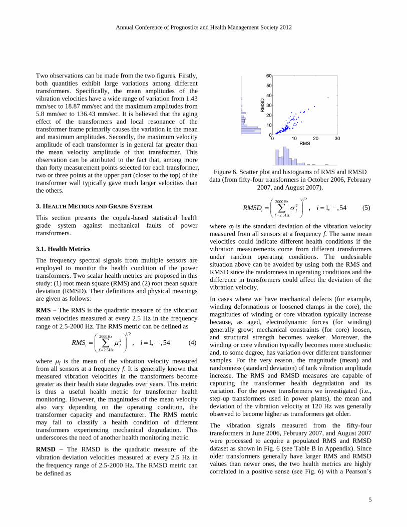
The vibration signals measured from the fifty-four
transformers in June 2006, February 2007, and August 2007
were processed to acquire a populated RMS and RMSD
dataset as shown in Fig. 6 (see Table B in Appendix). Since
older transformers generally have larger RMS and RMSD
values than newer ones, the two health metrics are highly
correlated in a positive sense (see Fig. 6) with a Pearson’s
Figure 6. Scatter plot and histograms of RMS and RMSD
data (from fifty-four transformers in October 2006, February
2007, and August 2007).
Annual Conference of Prognostics and Health Management Society 2012
6
linear correlation coefficient ρ being 0.9161. The
transformers with a relatively good health condition are
located at the lower left corner and the others at the upper
right corner.
3.2. Copula-Based Statistical Health Grade System
As shown in Fig. 6, a strong statistical correlation exists
between the proposed health metrics, RMS and RMSD. In
what follows, we intend to exploit this correlation using a
joint statistical model, copulas. We start with a brief
introduction on copulas. Next, we present three popular
types of copulas. Finally, we detail the procedures to
construct an appropriate copula for dependence modeling
based on available data.
3.2.1. Introduction of Copulas
In statistics, a copula is defined by Roser (1999) as “a
function that joins or couples multivariate joint distribution
functions to their one-dimensional marginal distribution
functions”, or “multivariate distribution functions whose
one-dimensional margins are uniform on the interval [0,1]”.
In other words, a copula formulates a joint cumulative
distribution function (CDF) based on marginal CDFs and a
dependence structure. In the following description, we will
see that copulas allow one to decouple the univariate
marginal distribution modeling from multivariate
dependence modeling.
Let x = (x1, x2,…, xN) be an N-dimensional random vector
with real-valued random variables, F be an N-dimensional
CDF of x with continuous marginal CDFs F1, F2,…, FN.
Then according to Sklar’s theorem, there exists a unique N-
copula C such that
1 2 1 1 2 2, ,..., , ,...,N N NF x x x C F x F x F x (6)
It then becomes clear that a copula formulates a joint CDF
with the support of separate marginal CDFs and a
dependence structure. This decoupling between marginal
distribution modeling and dependence modeling is an
attractive property of copulas, since it leads to the
possibility of building a wide variety of multivariate
densities. In real applications, this possibility can be enabled
by employing different types of marginal CDFs or
dependence structures. Based on Eq. (6) and under the
assumption of differentiability, we can derive the joint
probability density function (PDF) of the random vector x,
expressed as
1 2 1 1 2 2
1
, ,..., , ,...,N N N
N
i
i
f x x x c F x F x F x
f x
(7)
where c is the joint PDF of the copula C. The above
equation suggests that a joint PDF of x can be constructed as
the product of its marginal PDFs and a copula PDF. The
PDF formulation in Eq. (7) is useful in formulating a
likelihood function and estimating the parameters of
marginal PDFs and a copula, as will be discussed later.
3.2.2. Copula Types
Various general types of dependence structures can be
represented, corresponding to various copula families. In
what follows, we will briefly introduce four popular copula
types, that is, Gaussian, Clayton, Frank, and Gumbel. More
detailed information on copula families can be found in
(Roser, 1999).
Let ui = Fi(xi), i = 1, 2,…, N, an N-dimensional Gaussian
copula with a linear correlation matrix Σ is defined as
1 1
1 2
1 2 1
, ,, , , |
, |G N N
N
u uC u u u
u
Σ
Σ (8)
where Φ denotes the joint CDF of an N-dimensional
standard normal distribution and Φ−1
denotes the inverse
CDF of a one-dimensional standard normal distribution. It is
noted that Σ is a symmetric matrix with diagonal elements
ρii being ones, for i = 1, 2…, N, and off-diagonal elements
ρij being the pair-wise correlations between the pseudo
Gaussian random variables zi = Φ−1
(ui) and zj = Φ−1
(uj), for i,
j = 1, 2…, N and i ≠ j.
Another popular copula family is an N-dimensional
Archimedean copula, defined as
1
1 2
1
, , , |N
A N i
i
C u u u u
(9)
where Ψα denotes a generator function with a correlation
parameter α and satisfies the following conditions:
02
2
1 0; lim ;
0; 0
uu
d du u
du du
(10)
Annual Conference of Prognostics and Health Management Society 2012
7
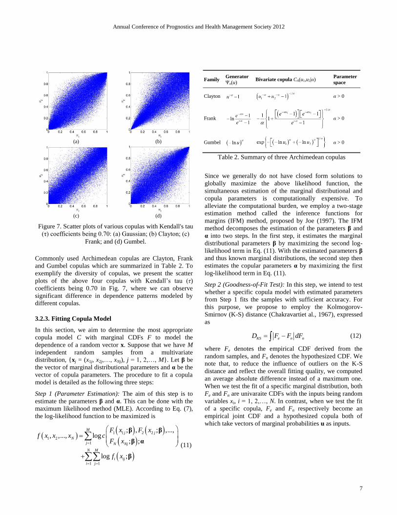
Commonly used Archimedean copulas are Clayton, Frank
and Gumbel copulas which are summarized in Table 2. To
exemplify the diversity of copulas, we present the scatter
plots of the above four copulas with Kendall’s tau (τ)
coefficients being 0.70 in Fig. 7, where we can observe
significant difference in dependence patterns modeled by
different copulas.
3.2.3. Fitting Copula Model
In this section, we aim to determine the most appropriate
copula model C with marginal CDFs F to model the
dependence of a random vector x. Suppose that we have M
independent random samples from a multivariate
distribution, {xj = (x1j, x2j,…, xNj), j = 1, 2,…, M}. Let β be
the vector of marginal distributional parameters and α be the
vector of copula parameters. The procedure to fit a copula
model is detailed as the following three steps:
Step 1 (Parameter Estimation): The aim of this step is to
estimate the parameters β and α. This can be done with the
maximum likelihood method (MLE). According to Eq. (7),
the log-likelihood function to be maximized is
1 1 2 2
1 2
1
1 1
; , ; ,...,, ,..., log
; ;
log ;
Mj j
N
j N Nj
N M
i ij
i j
F x F xf x x x c
F x
f x
β β
β α
β
(11)
Since we generally do not have closed form solutions to
globally maximize the above likelihood function, the
simultaneous estimation of the marginal distributional and
copula parameters is computationally expensive. To
alleviate the computational burden, we employ a two-stage
estimation method called the inference functions for
margins (IFM) method, proposed by Joe (1997). The IFM
method decomposes the estimation of the parameters β and
α into two steps. In the first step, it estimates the marginal
distributional parameters β by maximizing the second log-
likelihood term in Eq. (11). With the estimated parameters β
and thus known marginal distributions, the second step then
estimates the copular parameters α by maximizing the first
log-likelihood term in Eq. (11).
Step 2 (Goodness-of-Fit Test): In this step, we intend to test
whether a specific copula model with estimated parameters
from Step 1 fits the samples with sufficient accuracy. For
this purpose, we propose to employ the Kolmogorov-
Smirnov (K-S) distance (Chakravartiet al., 1967), expressed
as
KS e n nD F F dF (12)
where Fe denotes the empirical CDF derived from the
random samples, and Fn denotes the hypothesized CDF. We
note that, to reduce the influence of outliers on the K-S
distance and reflect the overall fitting quality, we computed
an average absolute difference instead of a maximum one.
When we test the fit of a specific marginal distribution, both
Fe and Fn are univaraite CDFs with the inputs being random
variables xi, i = 1, 2,…, N. In contrast, when we test the fit
of a specific copula, Fe and Fn respectively become an
empirical joint CDF and a hypothesized copula both of
which take vectors of marginal probabilities u as inputs.
Family Generator
Ψα(u) Bivariate copula CA(u1,u2|α)
Parameter
space
Clayton α > 0
Frank α > 0
Gumbel α > 0
Table 2. Summary of three Archimedean copulas
(a)
(b)
(c)
(d)
Figure 7. Scatter plots of various copulas with Kendall's tau
(τ) coefficients being 0.70: (a) Gaussian; (b) Clayton; (c)
Frank; and (d) Gumbel.

Annual Conference of Prognostics and Health Management Society 2012
8
Step 3 (Goodness-of-Fit Retest): To decide whether the
distance measure in Eq. (12) provides sufficient evidence on
the good fit of the copula, we retest the good-of-fit of the
copula model by generating random samples of the size M
under the assumption that the null hypothesis of an accurate
fit is true (Kole et al., 2007). We repeatedly execute the
retesting process K times to generate K sets of random
samples and, correspondingly, obtain K distance measures
by executing the aforementioned Steps 1 and 2. For each
retest, we generate random samples with two steps: (i)
generate sample pairs (u1j, u2j) of [0, 1] uniformed
distributed random variables u1j and u2 according to the
copula model with the parameters α estimated in Step 1; and
(ii) transform the sample pairs (u1j, u2j) to observation pairs
(x1j, x2j) with the inverse marginal CDFs F1−1
and F2−1
.
Finally, we construct a probability distribution of the
distance measure DKS and determine the p-value, or the
probability of observing a distance measure at least as
extreme as the value obtained in Step 2 under the
assumption of an accurate copula fit.
3.2.4. Building Copula-Based Statistical Health Grade
System
In this section, we apply the aforementioned copula model
to representing the joint distribution of the RMS and RMSD
metrics by modeling the dependence between these two.
Upon the construction of the joint distribution, we then
define a statistical health grade system based on the joint
CDF of the two health metrics.
a) Data Statistics and Marginal Distributions
Table 3 presents summary statistics on the populated RMS
and RMSD data as well as the types and parameters of fitted
marginal distributions. Compared to the RMS, the RMSD
yields a larger mean value and a much larger variance.
Kurtosis values are very high for both metrics, indicating
that a large portion of the variance is contributed to by
infrequent extreme deviations. This can also be observed
from the histograms of the two metrics in Fig. 8, where we
observe a considerable amount of extreme data for any of
the two metrics. Results from the K-S test suggest that the
RMS and RMSD data be statistically modeled with the
Weibull and gamma distributions, respectively. Parameters
of the fitted marginal distributions are given in Table 3 and
their plots are presented in Fig. 8.
b) Copula Model
We used the aforementioned procedure to identify an
appropriate copula model from the four candidates, that is,
Gaussian, Clayton, Frank and Gumbel copulas. Table 4
summarizes the copula fitting results based on the populated
RMS and RMSD data. Both the correlation estimate in
Gaussian copula and α estimates in three Archimedean
copulas indicate a strong correlation between the RMS and
RMSD. Regarding the retest, we generated 10,000 sets (i.e.,
K = 10,000) of random samples under the null hypothesis of
an accurate copula fit and ran each of the 10,000 sets
through the aforementioned Step 1 (Parameter Estimation)
and Step 2&3 (Goodness-of-Fit Test & Retest) to obtain
10,000 distance measures. It can be observed that any of the
four copulas cannot be rejected under the commonly used
significance level 0.05. This can be partially attributed to the
fact that we only have a relatively small number of data. We
conjecture that, as we have more data, the p-values yielded
by different copulas will become more distinctive and an
appropriate copula model can be selected with more
confidence. Out of the four copulas, Gaussian copula
produced the smallest distance measure DKS and the largest
p-value, which offers us a supporting evidence of the best fit
provided by Gaussian copula. The histogram of DKS of
Gaussian copula is plotted with the estimated DKS in Fig.
9(a). To verify the accuracy of fit, we synthetically
generated 1000 random samples from the fitted Gaussian
copula model and plot these samples together with the raw
Health
metric
Data statistics
Mean Stda Skewness Kurtosis Minimum Maximum
RMS 6.57 3.81 1.66 7.99 1.51 25.68
RMSD 8.27 6.64 1.64 6.04 1.20 37.63
Health
metric
Fitted marginal distribution
Type Parametersb
RMS Weibull 1 = 7.42, 2 = 1.84
RMSD Gamma 3 = 1.78, 4 = 4.64
a Standard deviation b Scale and shape parameters for Weibull and gamma distributions
Table 3. Summary of data statistics and fitted marginal
distributions
(a)
(b)
Figure 8. Histograms and fitted distributions of RMS (a) and
RMSD (b).

Annual Conference of Prognostics and Health Management Society 2012
9
data in Fig. 9(b). We can observe a generally accuracy
representation of the raw data, especially in the lower-left
region. The synthetic samples were generated by following
the same steps we used to generate the 10,000 random sets
for the retest: first drawing uniform samples from the copula
and then transforming these samples back to the original
Weibull and gamma samples using the inverse CDFs of
these distributions.
c) Health Grade System
We quantify the health condition for a specific transformer
unit (i.e., a specific RMS and RMSD pair) by the proportion
of the population with larger RMS and RMSD values than
that unit. Let x1 and x2 denote the health metrics RMS and
RMSD, respectively. Let C(F1(x1), F2(x2)) denote the copula
model we derived from the previous section with F1(x1) and
F2(x2) being the marginal CDFs of of x1 and x2.
Mathematically, the health condition h of an health metric
pair (x1d,x2d) can be defined in terms of marginal CDFs and
a joint CDF or copula, expressed as
1 2 1 1 2 2, Pr ,d d d dh x x x x x x
(13)
This can be further derived as a function of the marginal
CDFs of x1 and x2 and the copula, expressed as
1 2 1 1 1 2 2 2
1 1 1 2 2 2
1 1 1 2 2 2
1 1 2 2 1 1 2 2
, Pr ,
Pr Pr
Pr ,
1 ,
d d d d
d d
d d
d d d d
h x x u F x u F x
u F x u F x
u F x u F x
F x F x C F x F x
(14)
It is noted that, in the above equation, we define the health
condition of a transformer unit as the probability of a joint
event rather than a union one. The aim of this definition is to
achieve a certain level of conservativeness since the
mechanical failure of a power transformer causes significant
monetary and societal losses and is rather undesirable.
Based on the health condition defined in Eq. (14), we
further defined three health grades which, from the
perspective of probability, can be mapped to three ranges in
a zero-mean normal distribution, that is, below 1.0,
between 1.0 and 2.0 and above 2.0, as shown in Table 5.
Table 6 relates the three health grades to suggested
maintenance actions. Experts’ experience and historic
information on inspection and maintenance of the power
transformers over years were employed to derive the
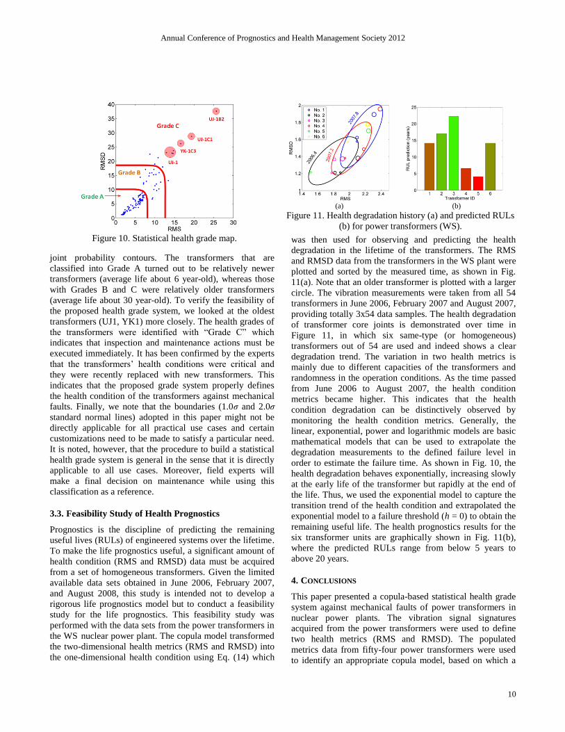
relationship. Fig. 10 visualizes the three health grades in the
RMS-RMSD map, where the boundaries were identified by
equating the health condition in Eq. (14) to the two critical
health conditions in Table 5 and deriving the corresponding
Copula
type
Parameter estimationa Test and retest
Point
estimate
Standard
error
95% confidence
intervalb DKS estimate p-valuec
Gaussian 0.930 0.012 (0.906, 0.955) 0.0300 0.3684
Clayton 6.035 0.688 (4.685,7.385)
0.0330 0.3216
Frank 15.095 1.384 (12.382,17.809)
0.0324 0.2916
Gumbel 3.484 0.194 (3.103,3.864) 0.0326 0.2642 a Linear correlation coefficient for Gaussian, α in Table 2 for the rest b Point estimate ± 1.96standard error c With 10,000 simulations
Table 4. Copula fitting results
(a)
(b)
Figure 9. Histograms of DKS (a) and scatter plot (b) of
Gaussian copula.
Health Grade A B C
Health condition h > 0.16 0.02 < h ≤ 0.16 h ≤ 0.02
-level of standard
normal distribution z < 1.0 1.0 ≤ z < 2.0 z ≥ 2.0
Table 5. Definition of three health grades
Health
Grade Health Conditions and Suggested Maintenance Actions
Grade A (Healthy)
Excellent health condition – Health condition is excellent;
transformer requires least frequent inspection and
maintenance.
Grade B
(Warning)
Transitional health condition – Health condition has partial
degradation; transformer requires more frequent inspection
(e.g., in-situ monitoring) to obtain health metric data that can be related to health condition; condition-based
maintenance (CBM) should be considered on the basis of
remaining useful life (RUL) prediction by health prognostics.
Grade C
(Faulty)
Critical health condition – Health condition is close to
failure due to mechanical faults in a component level; field engineers need to identify fault type, location, and severity;
transformer requires an immediate replacement of faulty
mechanical components to avoid entire transformer failure if they can be identified.
Table 6. Maintenance actions on health grades
Annual Conference of Prognostics and Health Management Society 2012
10
joint probability contours. The transformers that are
classified into Grade A turned out to be relatively newer
transformers (average life about 6 year-old), whereas those
with Grades B and C were relatively older transformers
(average life about 30 year-old). To verify the feasibility of
the proposed health grade system, we looked at the oldest
transformers (UJ1, YK1) more closely. The health grades of
the transformers were identified with “Grade C” which
indicates that inspection and maintenance actions must be
executed immediately. It has been confirmed by the experts
that the transformers’ health conditions were critical and
they were recently replaced with new transformers. This
indicates that the proposed grade system properly defines
the health condition of the transformers against mechanical
faults. Finally, we note that the boundaries (1.0σ and 2.0σ
standard normal lines) adopted in this paper might not be
directly applicable for all practical use cases and certain
customizations need to be made to satisfy a particular need.
It is noted, however, that the procedure to build a statistical
health grade system is general in the sense that it is directly
applicable to all use cases. Moreover, field experts will
make a final decision on maintenance while using this
classification as a reference.
3.3. Feasibility Study of Health Prognostics
Prognostics is the discipline of predicting the remaining
useful lives (RULs) of engineered systems over the lifetime.
To make the life prognostics useful, a significant amount of
health condition (RMS and RMSD) data must be acquired
from a set of homogeneous transformers. Given the limited
available data sets obtained in June 2006, February 2007,
and August 2008, this study is intended not to develop a
rigorous life prognostics model but to conduct a feasibility
study for the life prognostics. This feasibility study was
performed with the data sets from the power transformers in
the WS nuclear power plant. The copula model transformed
the two-dimensional health metrics (RMS and RMSD) into
the one-dimensional health condition using Eq. (14) which
was then used for observing and predicting the health
degradation in the lifetime of the transformers. The RMS
and RMSD data from the transformers in the WS plant were
plotted and sorted by the measured time, as shown in Fig.
11(a). Note that an older transformer is plotted with a larger
circle. The vibration measurements were taken from all 54
transformers in June 2006, February 2007 and August 2007,
providing totally 3x54 data samples. The health degradation
of transformer core joints is demonstrated over time in
Figure 11, in which six same-type (or homogeneous)
transformers out of 54 are used and indeed shows a clear
degradation trend. The variation in two health metrics is
mainly due to different capacities of the transformers and
randomness in the operation conditions. As the time passed
from June 2006 to August 2007, the health condition
metrics became higher. This indicates that the health
condition degradation can be distinctively observed by
monitoring the health condition metrics. Generally, the
linear, exponential, power and logarithmic models are basic
mathematical models that can be used to extrapolate the
degradation measurements to the defined failure level in
order to estimate the failure time. As shown in Fig. 10, the
health degradation behaves exponentially, increasing slowly
at the early life of the transformer but rapidly at the end of
the life. Thus, we used the exponential model to capture the
transition trend of the health condition and extrapolated the
exponential model to a failure threshold (h = 0) to obtain the
remaining useful life. The health prognostics results for the
six transformer units are graphically shown in Fig. 11(b),
where the predicted RULs range from below 5 years to
above 20 years.
4. CONCLUSIONS
This paper presented a copula-based statistical health grade
system against mechanical faults of power transformers in
nuclear power plants. The vibration signal signatures
acquired from the power transformers were used to define
two health metrics (RMS and RMSD). The populated
metrics data from fifty-four power transformers were used
to identify an appropriate copula model, based on which a
Figure 10. Statistical health grade map.
(a)
(b)
Figure 11. Health degradation history (a) and predicted RULs
(b) for power transformers (WS).

Annual Conference of Prognostics and Health Management Society 2012
11
statistical health grade system is built with corresponding
health conditions and suggested maintenance actions. The
copula-based statistical health grade system can be useful
for making maintenance decisions, while monitoring the
health conditions of the power transformers. It is noted that
uncertainties in manufacturing conditions, operation
conditions and measurements further propagate to
uncertainties in the two health metrics. Thus, a health grade
system should not only be characterized by its diagnostic
accuracy but also by its ability to perform the diagnostics in
a statistical manner. In this light, the proposed statistical
health grade system offer researchers and industrial
practitioner a powerful tool to systematically capture the
aforementioned uncertainties and build statistical power in
defining health grades. To investigate the feasibility of the
proposed statistical health grade system for health
prognostics, we established an exponential model to capture
the transition trend of the health condition and predicted the
remaining useful life by extrapolation. Finally, we conclude
that the copula model is capable of characterizing the
statistical dependence between the two health metrics, and
that the health condition defined based on this model is an
attractive health measure suitable for health prognostics.
APPENDIX
Location Unit Type Manufacture Voltage
(High/Low, kV)
Capacity
(MVA, at
55oC)
KORI 1 3 phase hyosung 362/22 750
2 3 phase hyosung 362/22 790
3 1 phase hyosung 362/22 385 * 3
4 1 phase hyosung 362/22 385 * 3
YK
1 1 phase hyosung 362/22 403 * 3
2 1 phase hyosung 362/22 403 * 3
3 1 phase hyosung 345/20.9 353.3 * 3
4 1 phase hyosung 345/20.9 353.3 * 3
5 1 phase hyosung 345/20.9 353.3 * 3
6 1 phase hyosung 345/20.9 353.3 * 3
WS
1 3 phase Hyundai 362/26 840
2 1 phase Hyundai 345/22 277 * 3
3 1 phase Hyundai 345/22 277 * 3
4 1 phase Hyundai 345/22 277 * 3
UJ
1 1 phase hyosung 362/22 372.8 * 3
2 1 phase hyosung 362/22 372.8 * 4
3 1 phase hyosung 345/20.9 353.3 * 3
4 1 phase hyosung 345/20.9 353.3 * 3
5 1 phase hyosung 345/20.9 353.3 * 3
6 1 phase hyosung 345/20.9 353.3 * 3
Table A. Specifications for transformers in KORI, YK, UJ,
and WS.
Location Unit Phase 04/2006 02/2007 08/2007 RMS RMSD RMS RMSD RMS RMSD
YK 1 A
B 3.4935 3.7586 4.4083 4.7433
C 10.8184 21.2638 9.6774 15.2434 11.9149 18.7117
2 A 6.1644 8.0906 5.8147 7.4488 7.2082 9.1807
B 8.2268 18.4866 6.2618 14.3723 7.7437 17.7022
C 7.0891 11.9838 5.8223 7.8991 7.2067 9.7351
3 A 3.5302 2.6278 2.9425 2.3837 3.7121 3.0416
B 8.7348 22.4859 4.4078 7.0695 5.4724 8.7757
C 6.2146 8.1801 5.7957 3.7542 7.4235 4.8832
4 A 7.0048 7.9036 6.3626 9.68 8.0392 12.0284 B 5.8535 5.2815 4.4444 3.4313 5.5571 4.295
C 4.5239 3.5049 3.3184 3.4511 4.1653 4.2948
5 A 8.0345 6.1175 3.3179 3.0496 4.2151 3.8115 B 6.4082 6.0413 3.8493 4.6327 4.8549 5.7959
C 10.2612 15.3348 4.6928 6.6165 5.7945 8.1362
6 A 6.2767 6.7398 5.002 6.2901 6.1577 7.7343
B 6.3487 8.3477 6.9783 7.6711 8.5739 9.4235 C 6.3093 6.2303 6.2191 6.3663 7.6363 7.8104
UJ 1 A
B 25.683 37.6344 C 19.3516 28.7425 14.738 23.756 8.4941 14.8265
2 A 9.9755 19.0113 12.9438 23.0255 14.619 22.7439
B 11.0612 15.9743 8.6555 15.8371 11.9566 18.0058
C 14.3538 22.8637 9.2198 15.9236 7.2417 8.1277
3 A 6.1895 5.9806 10.0143 11.3763 6.5462 6.4366
B 11.4765 12.6484 13.4102 13.199 9.7375 10.0747
C 9.7347 17.1477 6.8758 9.2086 6.8016 6.0879
4 A 7.1267 12.411 6.1393 6.0104 7.8248 12.9405 B 4.6828 3.7881 6.0354 5.198 6.9082 6.2445
C 3.0354 3.976 6.1473 4.7841 6.8478 7.8904
5 A 6.8923 7.2407 5.1924 5.2341 6.7011 8.7737 B 11.0317 10.2376 9.4405 7.1195 10.4389 9.6835
C 5.7305 5.792 6.0117 6.5637 5.8994 5.8661
6 A 6.195 6.8874 7.1765 7.1809 7.5634 8.1893 B 6.1051 7.9166 5.114 4.7147 5.8188 10.0799
C 6.4567 6.1449 6.3587 6.4674 6.8919 7.2125
WS 1
2 A 1.5119 1.2139 2.2402 1.702 B 2.8317 2.6835
C 1.9431 1.3812 2.1804 1.4858 2.3866 1.9573
3 A 2.0948 1.5776 2.0962 1.6223 2.3091 1.8932
B 1.8853 1.2124 1.8178 1.2107 2.1066 1.3798 C 1.7767 1.207 1.8101 1.3677 1.9125 1.3735
4 A 2.3797 2.9213 2.3555 2.0227 2.3555 2.0227
B 2.0295 2.0761 2.4585 2.2441 2.4585 2.2441 C 1.9772 1.5718 2.2301 1.7756 2.2301 1.7756
Table B. RMS and RMSD for all transformers in YK, UJ,
and WS.
ACKNOWLEDGEMENT
This work was partially supported by a grant from the
Energy Technology Development Program of Korea
Institute of Energy Technology Evaluation and Planning
(KETEP), funded by the Korean government’s Ministry of
Knowledge Economy and by the SNU-IAMD.
REFERENCES
Bartoletti, C., Desiderio, M., Carlo, D., Fazio, G., Muzi, F.,
Sacerdoti, G., & Salvatori, F. (2004). Vibro-acoustic
Techniques to Diagnose Power Transformers. IEEE
Transactions on Power Delivery, v19, n1, p221–229.

Annual Conference of Prognostics and Health Management Society 2012
12
Chakravarti, M., Laha, R.G., & Roy, J., (1967). Handbook
of methods of applied statistics, volume I. John Wiley
and Sons, p392–394.
Dick, E.P., & Erven, C.C. (1978). Transformer Diagnostic
Testing by Frequency Response Analysis. IEEE
Transactions on Power Apparatus and Systems, vPAS-
97, n6, p2144–2153.
Fei, S.-W., Liu, C.-L., & Miao, Y.-B. (2009). Support
Vector Machine with Genetic Algorithm for
Forecasting of Key-gas Ratios in Oil-immersed
Transformer. Expert Systems with Applications, v36, n3,
p6326–6331.
Fei, S., & Zhang, X. (2009). Fault Diagnosis of Power
Transformer based on Support Vector Machine with
Genetic Algorithm. Expert Systems with Applications,
v36, n8, p11352–11357.
Garcia, B., Burgos, J.C., Alonso, A.M., & Sanz, J. (2005). A
Moisture-in-Oil Model for Power Transformer
Monitoring-Part II: Experimental Verification. IEEE
Transactions on Power Delivery, v20, n2, p1423–1429.
García, B., Member, Burgos, J.C., & Alonso Á .M. (2006).
Transformer Tank Vibration Modeling as a Method of
Detecting Winding Deformations—Part I: Theoretical
Foundation. IEEE Transactions on Power Delivery, v21,
n1, p157–163.
García B., Burgos J.C. & Alonso, Á .M. (2006). Transformer
Tank Vibration Modeling as a Method of Detecting
Winding Deformations—Part II: Experimental
Verification. IEEE Transactions on Power Delivery,
v21, n1, p164–169.
Gong, L., Liu, C-H., & Zha, X.F. (2007). Model-Based
Real-Time Dynamic Power Factor Measurement in AC
Resistance Spot Welding with an Embedded ANN.
IEEE Transactions on Industrial Electronics, v54, n3,
p1442–1448.
Hao, X., & Cai-xin, S. (2007). Artificial Immune Network
Classification Algorithm for Fault Diagnosis of Power
Transformer. IEEE Transactions on Power Delivery,
v22, n2, p930–935.
Hong-Tzer, Y., & Chiung-Chou, L. (1999). Adaptive Fuzzy
Diagnosis System for Dissolved Gas Analysis of Power
Transformers. IEEE Transactions on Power Delivery,
v14, n4, p1342–1350.
Huang, Y. C. (2003). Evolving Neural Nets for Fault
Diagnosis of Power Transformers. IEEE Transactions
on Power Delivery, v18, n3, p843–848.
IEEE std. C57.104 (2008). IEEE guide for the interpretation
of gases generated in oil-immersed transformers.
Ji, S., Luo, Y., & Li, Y. (2006). Research on Extraction
Technique of Transformer Core Fundamental
Frequency Vibration Based on OLCM. IEEE
Transactions on Power Delivery, v21, n4, p1981–1988.
Joe, H. (1997). Multivariate models and dependence
concepts: Monographs on Statistics and Applied
Probability, vol. 73. Chapman & Hall, London, UK.
Kole, E., Koedijk, K., & Verbeek, M. (2007). Selecting
Copulas for Risk Management. Journal of Banking and
Finance, v31, n8, p2405–2423.
Lee, W.R., Jung, S.W., Yang, K.H., & Lee, J.S. (2005). A
study on the determination of subjective vibration
velocity ratings of main transformers under operation in
nuclear power plants. In Proceedings of the 12th
International Congress on Sound and Vibration (Paper
No. 1017), July 11-14, Lisbon, Portugal,.
McArthur, S.D.J., Strachan, S.M., & Jahn, G. (2004). The
Design of a Multi-Agent Transformer Condition
Monitoring System. IEEE Transactions on Power
Delivery, v19, n4, p1845–1852.
Muhamad, N.A., & Ali, S.A.M. (2006). Simulation Panel
for Condition Monitoring of Oil and Dry Transformer
Using LabVIEW with Fuzzy Logic Controller. Journal
of Engineering, Computing & Technology, v14, p187–
193.
Picanço, A.F., Martinez, M.L.B., & Paulo, C.R. (2010).
Bragg System for Temperature Monitoring in
Distribution Transformers. Electric Power System
Research, v80, n1, p77–83.
Pradhan, M. K. (2006). Assessment of the Status of
Insulation during Thermal Stress Accelerated
Experiments on Transformer Prototypes. IEEE
Transactions on Dielectrics and Electrical Insulation,
v13, n1, p227–237.
Purkait, P., & Chakravorti, S. (2002). Time and Frequency
Domain Analyzes based Expert System for Impulse
Fault Diagnosis in Transformers. IEEE Transactions on
Dielectrics and Electrical Insulation, v9, n3, p433–445.
Roser, B.N. (1999). An Introduction to Copulas. New York:
Springer.
Saha, T. K., & Purkait, P. (2004). Investigation of an Expert
System for the Condition Assessment of Transformer
Insulation based on Dielectric Response Measurements.
IEEE Transactions on Power Delivery, vol. 19, no. 3,
p1127–1134.
Saha, T.K. (2003). Review of Modern Diagnostic
Techniques for Assessing Insulation Condition in Aged
Transformers. IEEE Transactions on Dielectrics and
Electrical Insulation, v10, n5, p903–917.
Shin, H.J., & Cho, S. (2006). Response Modeling with
Support Vector Machines. Expert Systems with
Applications, v30, n4, p746–760.
Su, Q., Mi, C., Lai, L.L., & Austin, P. (2000) A Fuzzy
Dissolved Gas Analysis Method for the Diagnosis of
Multiple Incipient Faults in a Transformer. IEEE
Transactions on Power Systems, v15, n2, p593–598.
Annual Conference of Prognostics and Health Management Society 2012
13
Tang, W.H., Wu, Q.H., & Richardson Z.J. (2004). A
Simplified Transformer Thermal Model Based on
Thermal-Electric Analogy. IEEE Transactions on
Power Delivery, v19, n3, p1112–1119.
Wang, M., Vandermaar, A. J., & Srivastava, K. D. (2002)
Review of condition assessment of power transformers
in service. IEEE Electrical Insulation Magazine, v18,
n6, p12–25.
Wang, P., Youn, B.D., & Hu, C. (2010). A generic sensor
network design framework based on a detectability
measure. ASME International Design Engineering
Technical Conferences & Computers and Information
in Engineering Conference, August 15- 18, Montreal,
Quebec, Canada.
BIOGRAPHIES
Chao Hu: Dr. Chao Hu is currently working
as a senior reliability engineer at Medtronic,
Inc. in Minneapolis, MN. He received his
B.E. degree in Engineering Physics from
Tsinghua University in Beijing, China in
2003, and the Ph.D. degree in mechanical
engineering at the University of Maryland,
College Park in USA. His research interests are system
reliability analysis, prognostics and health management
(PHM), and battery power and health management of Li-ion
battery system. Dr. Hu’s research work has led to more than
30 journal and conference publications in the above areas.
Pingfeng Wang: Dr. Pingfeng Wang
received his B.E. degree in Mechanical
Engineering from The University of Science
and Technology in Beijing, China in 2001,
the M.S. degree in Applied Mathematics in
Tsinghua University in Beijing, China in
2006, and the Ph.D. degree in mechanical
engineering at the University of Maryland, College Park in
USA. He is currently an Assistant Professor in the
Department of Industrial and Manufacturing Engineering at
Wichita State University. His research interests are system
reliability analysis, risk-based design, and prognostics and
health management (PHM).
Byeng D. Youn: Dr. Byeng D. Youn
received his Ph.D. degree from the
department of Mechanical Engineering at
the University of Iowa, Iowa City, IA, in
2001. He was a research associate at the
University of Iowa (until 2004), an assistant
professor in Michigan Technical University
(until 2007), and an assistant professor in the
University of Maryland College Park (until 2010). Currently,
he is an assistant professor at the School of Mechanical and
Aerospace Engineering at Seoul National University,
Republic of Korea. His research is dedicated to well-
balanced experimental and simulation studies of system
analysis and design, and he is currently exploring three
research avenues: system risk-based design, prognostics and
health management (PHM), and energy harvester design. Dr.
Youn’s research and educational dedication has led to: six
notable awards, including the ISSMO/Springer Prize for the
Best Young Scientist in 2005 from the International Society
of Structural and Multidisciplinary Optimization (ISSMO),
and more than 100 publications in the area of system-risk-
based design and PHM and energy harvester design.
Wook-Ryun Lee: Mr. Wook-Ryun Lee
received his Master’s degree in Mechanical
Engineering from Chungnam National
University in 2004 and his Bachelor’s
degree from Yonsei University in 1997. He
is currently a senior researcher in the Green
Energy Laboratory of the Research Institute
in the Korea Electric Power Corporation, Daejeon, Korea.
His research interests are control of noise and vibration
generated from power plants, and kinetic energy storage
system such as flywheel energy storage, energy-harvesting
etc.
Joung Taek Yoon: Mr. Joung Taek Yoon
received his B.S. degree in mechanical
engineering from Seoul National University
in 2011 and is currently pursuing a combined
master's and doctorate program in
mechanical engineering from Seoul National
University. His research interests are
prognostics and health management (PHM) and resilient
system design.


