
The Influence of In Situ Reheat on Turbine-Combustor Performance (GT2004-54071)
Steven Chambers, Horia Flitan, Paul Cizmas1
Department of Aerospace Engineering
Texas A&M University
College Station, Texas 77843
Dennis Bachovchin, Thomas Lippert
Siemens-Westinghouse Power Corporation
Pittsburgh, Pennsylvania 15235
David Little
Siemens-Westinghouse Power Corporation
Orlando, Florida 32826
Abstract
This paper presents a numerical and experimental investigation of the in situ reheat necessary for
the development of a turbine-combustor. The flow and combustion were modeled by the Reynolds-
averaged Navier-Stokes equations coupled with the species conservation equations. The chemistry model
used herein was a two-step, global, finite rate combustion model for methane and combustion gases.
A numerical simulation was used to investigate the validity of the combustion model by comparing
the numerical results against experimental data obtained for an isolated vane with fuel injection at its
trailing edge. The numerical investigation was then used to explore the unsteady transport phenomena
in a four-stage turbine-combustor. In situ reheat simulations investigated the influence of various fuel
injection parameters on power increase, airfoil temperature variation and turbine blade loading. The in
situ reheat decreased the power of the first stage, but increased more the power of the following stages,
such that the power of the turbine increased between 2.8% and 5.1%, depending on the parameters of the
fuel injection. The largest blade excitation in the turbine-combustor corresponded to the fourth-stage
rotor, with or without combustion. In all cases analyzed, the highest excitation corresponded to the first
blade passing frequency.
1To whom correspondence should be addressed.
Introduction
In the attempt to increase the thrust-to-weight ratio and decrease the thrust specific fuel consumption,
turbomachinery designers are facing the fact that the combustor residence time can become shorter than the
time required to complete combustion. As a result, combustion could continue in the turbine, which is often
considered to be undesirable. A thermodynamic cycle analysis, however, demonstrated a long time ago the
benefits of using reheat in the turbine in order to increase specific power and thermal efficiency. Even better
performance gains for specific power and thermal efficiency were predicted for power generation gas-turbine
engines when the turbine is coupled with a heat regenerator [1]. Starting in the 1960s, several patents were
awarded for different inventions that addressed various aspects related to turbine reheat [2, 3, 4].
In spite of these advances, the technological challenges and the difficulty of predicting and understanding
the details of the transport phenomena inside the reheat turbine precluded the development of turbine-
combustors. Herein, a turbine-combustor is defined as a turbine in which fuel is injected and combustion
takes place. The process of combustion in the turbine is called in situ reheat.
Several challenges are associated with the combustion in the turbine-burner: mixed subsonic and super-
sonic flows; flows with large unsteadiness due to the rotating blades; hydrodynamic instabilities and large
straining of the flow due to the very large three-dimensional acceleration and stratified mixtures [1]. The
obvious drawback associated with the strained flows in the turbine-burner is that widely varying velocities
can result in widely varying residence time for different flow paths and, as a result, there are flammability
difficulties for regions with shorter residence times. In addition, transverse variation in velocity and kinetic
energy can cause variations in entropy and stagnation entropy that impact heat transfer. The heat transfer
and mixing may be enhanced by increasing interface area due to strained flows.
Experimental data for conventional (i.e., without in situ reheat) gas-turbines have shown the existence
of large radial and circumferential temperature gradients downstream of the combustor [5, 6]. These tem-
perature non-uniformities, called hot streaks, have a significant impact on the secondary flow and wall
temperature of the entire turbine. Since the combustor exit flow may contain regions where the temperature
exceeds the allowable metal temperature by 460-930 K [7], understanding the effects of temperature non-
uniformities on the flow and heat transfer in the turbine is essential for increasing vane and blade durability.
GTP-04-1149 2 Cizmas

It is estimated that an error of 100 K in predicting the time-averaged temperature on a turbine rotor can
result in an order of magnitude change in the blade life [8, 9].
Temperature non-uniformities generated by the upstream combustor can be amplified in a turbine-burner.
Consequently, it is expected that not only will the secondary flow and wall temperature be affected but also
the blade loading due to the modified pressure distribution. Temperature non-uniformities in a turbine-
burner can also affect the location of hot spots on airfoils and, as a result, can affect the internal and film
cooling schemes.
Numerous experimental [10, 11, 12, 7, 13, 14] and numerical [15, 16, 17, 18, 19] investigations explored
the influence of temperature non-uniformities on the flow and heat transfer in a conventional turbine. To
the best knowledge of the authors, there are no data, however, available in the open literature that illustrate
the effects of in situ reheat on turbine-burners. The objective of this paper is to evaluate a numerical model
for in situ reheat against experimental data for a single vane-burner and to use this numerical model to
investigate the effects of combustion on the performance of a four-stage turbine-combustor. This numerical
simulation is crucial for the development of turbine-burners which, in spite of their challenges, can provide
significant performance gains for turbojet engines and power generation gas-turbine engines.
The next section presents the physical model used for the simulation of flow and combustion in a turbine-
combustor. The governing equations and the chemistry model are presented. The third section describes
the numerical model. This section includes information about the grid generation, boundary conditions, and
numerical method. The comparison against experimental data and the results for a four-stage turbine are
presented in the fourth section.
Physical Model
The effects of in situ reheat on (1) a single vane-burner, and (2) a multi-row turbine-burner are modeled
by the Reynolds-averaged Navier-Stokes equations and the species conservation equations. The model is
three-dimensional for the single vane, and quasi-three-dimensional for the four-stage turbine-combustor, in
order to reduce the computational time. This section will present the details of the governing equations and
the chemistry model.
GTP-04-1149 3 Cizmas

Governing Equations
The unsteady, compressible flow through the turbine-combustor was modeled by the Reynolds-averaged
Navier-Stokes equations. The flow was assumed to be fully turbulent and the kinematic viscosity is computed
using Sutherland’s law. The Reynolds-averaged Navier-Stokes equations and species conservation equations
were simplified by using the thin-layer assumption [20].
In the hypothesis of unity Lewis number, both the Reynolds-averaged Navier-Stokes and species equations
were written as [21]:
∂Q
∂τ+
∂F
∂ξ+
∂G
∂η=
√γ∞M∞
Re∞
∂S
∂η+ Sch. (1)
Note that equation (1) was written in the body-fitted curvilinear coordinate system (ξ, η, τ).
The state and flux vectors of the Reynolds-averaged Navier-Stokes equations in the Cartesian coordinates
were
qns =
ρ
ρu
ρv
e
, fns =
ρu
ρu2 + p
ρuv
(e + p)u
, gns =
ρv
ρuv
ρv2 + p
(e + p) v
.
The state and flux vectors of the species conservation equations in the Cartesian coordinates were
qsp =
ρy1
ρy2
...
ρyN
, fsp =
ρuy1
ρuy2
...
ρuyN
, gsp =
ρvy1
ρvy2
...
ρvyN
.
Further details on the description of the viscous terms and chemical source terms are presented in [22].
GTP-04-1149 4 Cizmas

Chemistry Model
The purpose of this investigation was to determine the influence of in situ reheat on the performance of
a turbine-combustor, as opposed to predicting the complete set of combustion products. Consequently,
the chemistry model used herein was a two-step, global, finite rate combustion model for methane and
combustion gases [23, 24]
CH4 + 1.5O2 → CO + 2H2O
CO + 0.5O2 → CO2.
(2)
This reduced kinetics model was tuned to match the flame speed and heat released, as opposed to species
concentrations [23]. The rate of progress (or Arrhenius-like reaction rate) for methane oxidation was given
by:
q1 = A1 exp (−E1/R/T ) [CH4]−0.3
[O2]1.3
, (3)
where A1 = 2.8 · 109 s−1, E1/R = 24360 K. The reaction rate for the CO/CO2 equilibrium was:
q2 = A2 exp (−E2/R/T ) [CO] [O2]0.25
[H2O]0.5
(4)
with A2 = 2.249 · 1012(
m3/kmol)0.75
s−1 and E2/R = 20130 K. The symbols in the square brackets
represent local molar concentrations of various species. The net formation/destruction rate of each species
due to all reactions was ˆwi =∑Nr
k=1Miνikqk, where νik were the generalized stoichiometric coefficients.
Note that the generalized stoichiometric coefficient is νik = ν′′
ik − ν′
ik, where ν′
ik and ν′′
ik are stoichiometric
coefficients in reaction k for species i appearing as a reactant or as a product. Additional details on the
implementation of the chemistry model can be found in [20].
GTP-04-1149 5 Cizmas
Numerical Model
The numerical model used herein to simulate the flow and combustion in the four-stage turbine-combustor
was implemented in the CoRSI code [20] and was based on an algorithm developed for unsteady flows in
turbomachinery [25]. The Reynolds-averaged Navier-Stokes equations and the species equations were written
in strong conservation form. The fully implicit, finite-difference approximation was solved iteratively at each
time level, using an approximate factorization method. Three Newton-Raphson sub-iterations were used to
reduce the linearization and factorization errors at each time step. The convective terms were evaluated using
a third-order accurate upwind-biased Roe scheme [26]. The viscous terms were evaluated using second-order
accurate central differences. The scheme was second-order accurate in time.
The size of the computational domain used to simulate the flow inside the turbine-combustor was reduced
by taking into account flow periodicity. Two types of grids were used to discretize the flow field surrounding
the rotating and stationary airfoils, as shown in Fig. 10. An O-grid was used to resolve the governing
equations near the airfoil, where the viscous effects were important. An H-grid was used to discretize the
governing equations away from the airfoil. The O-grid was generated using an elliptical method. The H-grid
was algebraically generated. The O- and H-grids were overlaid. The flow variables were communicated
between the O- and H-grids through bilinear interpolation. The H-grids corresponding to consecutive rotor
and stator airfoils were allowed to slip past each other to simulate the relative motion.
The transport of chemical species was modeled by the mass, momentum, energy and species balance
equations. The governing equations of gas-dynamics and chemistry were solved using a fully decoupled
implicit algorithm [27, 28, 21, 29]. A correction technique was developed to enforce the balance of mass
fractions [20]. The governing equations were discretized using an implicit, approximate-factorization, finite
difference scheme in delta form [30]. The discretized operational form of both the Reynolds-averaged Navier-
Stokes and species conservation equations, combined in a Newton-Raphson algorithm [31], were described
in [20, 22] where additional details on the implementation of the inter-cell numerical fluxes and on the Roe’s
approximate Riemann solver were presented.
Two classes of boundary conditions were enforced on the grid boundaries: (1) natural boundary condi-
tions, and (2) zonal boundary conditions. The natural boundaries included inlet, outlet, periodic and the
GTP-04-1149 6 Cizmas

airfoil surfaces. The zonal boundaries included the patched and overlaid boundaries.
At the inlet boundary conditions, the flow angle, average total pressure and downstream propagating
Riemann invariant were specified. The upstream propagating Riemann invariant was extrapolated from
the interior of the domain. At the outlet, the average static pressure was specified, while the downstream
propagating Riemann invariant, circumferential velocity, and entropy were extrapolated from the interior of
the domain. Periodicity was enforced by matching flow conditions between the lower surface of the lowest
H-grid of a row and the upper surface of the top most H-grid of the same row. At the airfoil surface, the
following boundary conditions were enforced: the “no slip” condition, the adiabatic wall condition, and the
zero normal pressure gradient condition.
Data were transferred from the H-grid to the O-grid along the O-grid’s outermost grid line to impose
the zonal boundary conditions of the overlaid boundaries. Data were then transferred back to the H-grid
along its inner boundary. At the end of each iteration, an explicit, corrective, interpolation procedure was
performed. The patch boundaries were treated similarly, using linear interpolation to update data between
adjoining grids [32].
Results
This section starts with the evaluation of the combustion model against experimental data for a single-vane
burner. Selected results of the numerical simulation of unsteady transport phenomena inside a four-stage
turbine-combustor are subsequently presented. The section describing the four-stage turbine-combustor
begins with a description of the geometry and flow conditions, followed by a brief discussion of the accuracy
of numerical results. The last part of this section presents the effects of in situ reheat on the unsteady flow,
blade loading and power increase in the turbine-combustor.
Single-Vane Burner
To verify the validity of the methane combustion model for in situ reheat applications, a single-vane burner
was experimentally investigated and numerically simulated. In-situ reheat tests were run in the Siemens
Westinghouse small-scale, full-pressure, combustion test facility, shown in Fig. 1. Preheated air (0.20 kg/s)
GTP-04-1149 7 Cizmas

and natural gas were delivered to a low-NOx burner section, which was run at full pressure (typically 14 bar).
Air preheat temperature and fuel/air ratio were adjusted to give an exhaust gas stagnation temperature and
composition corresponding to a selected location in a turbine cascade. The exhaust gas was then passed
through a pressure-reducing orifice to increase the Mach number in the injection and sampling sections to
typical turbine levels. A back pressure control valve was used to set the sampling section pressure.
Figure 1: Experimental setup for a single-vane burner.
Using a calibrated orifice plate, air flow to the system was measured with an accuracy of 2%. Natural
gas flow was regulated with a mass flow controller with an accuracy of 1%. Gases were sampled at various
locations downstream of the injection point, and compositions determined using a gas chromatograph, with
error limits of ±5%. The temperature was measured with thermocouples, with error limits of ±2 K. Upstream
of the vane-burner, the mass flow rate of gases was 0.134 kg/s, the total temperature was 1507 K and the
total pressure was 6.26 bar. The vane-burner was placed in a 17.8 mm by 25.4 mm pipe. The 17.8 mm
by 25.4 mm pipe reduces to a 17.8 mm by 17.8 mm pipe at approximately 69.8 mm downstream from the
vane-burner, as shown in Fig. 2. The static pressure upstream of the 17.8 mm by 17.8 mm pipe was 5.44
GTP-04-1149 8 Cizmas
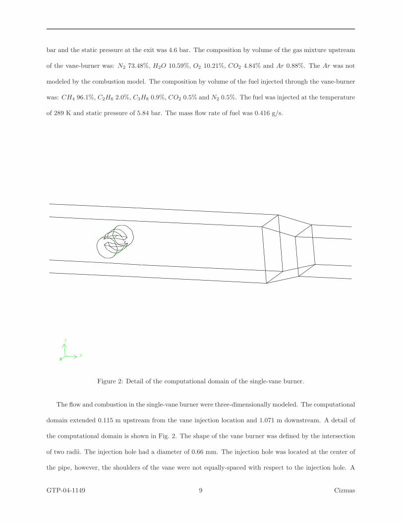
bar and the static pressure at the exit was 4.6 bar. The composition by volume of the gas mixture upstream
of the vane-burner was: N2 73.48%, H2O 10.59%, O2 10.21%, CO2 4.84% and Ar 0.88%. The Ar was not
modeled by the combustion model. The composition by volume of the fuel injected through the vane-burner
was: CH4 96.1%, C2H6 2.0%, C3H8 0.9%, CO2 0.5% and N2 0.5%. The fuel was injected at the temperature
of 289 K and static pressure of 5.84 bar. The mass flow rate of fuel was 0.416 g/s.
X
Y
Z
Figure 2: Detail of the computational domain of the single-vane burner.
The flow and combustion in the single-vane burner were three-dimensionally modeled. The computational
domain extended 0.115 m upstream from the vane injection location and 1.071 m downstream. A detail of
the computational domain is shown in Fig. 2. The shape of the vane burner was defined by the intersection
of two radii. The injection hole had a diameter of 0.66 mm. The injection hole was located at the center of
the pipe, however, the shoulders of the vane were not equally-spaced with respect to the injection hole. A
GTP-04-1149 9 Cizmas
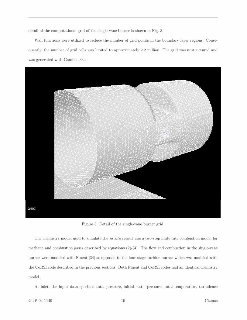
detail of the computational grid of the single-vane burner is shown in Fig. 3.
Wall functions were utilized to reduce the number of grid points in the boundary layer regions. Conse-
quently, the number of grid cells was limited to approximately 2.2 million. The grid was unstructured and
was generated with Gambit [33].
Grid
Z
Y
X
Figure 3: Detail of the single-vane burner grid.
The chemistry model used to simulate the in situ reheat was a two-step finite rate combustion model for
methane and combustion gases described by equations (2)-(4). The flow and combustion in the single-vane
burner were modeled with Fluent [34] as opposed to the four-stage turbine-burner which was modeled with
the CoRSI code described in the previous sections. Both Fluent and CoRSI codes had an identical chemistry
model.
At inlet, the input data specified total pressure, initial static pressure, total temperature, turbulence
GTP-04-1149 10 Cizmas
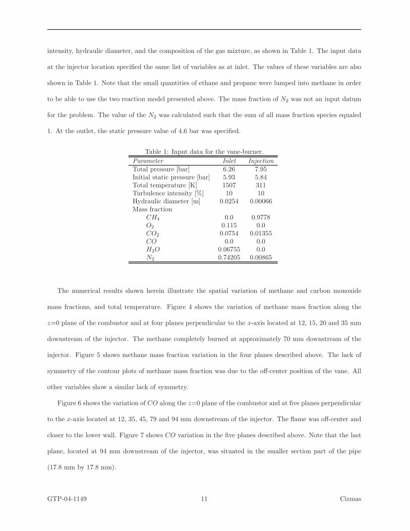
intensity, hydraulic diameter, and the composition of the gas mixture, as shown in Table 1. The input data
at the injector location specified the same list of variables as at inlet. The values of these variables are also
shown in Table 1. Note that the small quantities of ethane and propane were lumped into methane in order
to be able to use the two reaction model presented above. The mass fraction of N2 was not an input datum
for the problem. The value of the N2 was calculated such that the sum of all mass fraction species equaled
1. At the outlet, the static pressure value of 4.6 bar was specified.
Table 1: Input data for the vane-burner.
Parameter Inlet Injection
Total pressure [bar] 6.26 7.95Initial static pressure [bar] 5.93 5.84Total temperature [K] 1507 311Turbulence intensity [%] 10 10Hydraulic diameter [m] 0.0254 0.00066Mass fraction
CH4 0.0 0.9778O2 0.115 0.0CO2 0.0754 0.01355CO 0.0 0.0H2O 0.06755 0.0N2 0.74205 0.00865
The numerical results shown herein illustrate the spatial variation of methane and carbon monoxide
mass fractions, and total temperature. Figure 4 shows the variation of methane mass fraction along the
z=0 plane of the combustor and at four planes perpendicular to the x-axis located at 12, 15, 20 and 35 mm
downstream of the injector. The methane completely burned at approximately 70 mm downstream of the
injector. Figure 5 shows methane mass fraction variation in the four planes described above. The lack of
symmetry of the contour plots of methane mass fraction was due to the off-center position of the vane. All
other variables show a similar lack of symmetry.
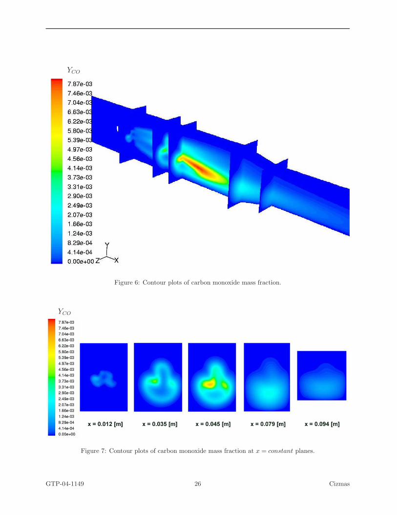
Figure 6 shows the variation of CO along the z=0 plane of the combustor and at five planes perpendicular
to the x-axis located at 12, 35, 45, 79 and 94 mm downstream of the injector. The flame was off-center and
closer to the lower wall. Figure 7 shows CO variation in the five planes described above. Note that the last
plane, located at 94 mm downstream of the injector, was situated in the smaller section part of the pipe
(17.8 mm by 17.8 mm).
GTP-04-1149 11 Cizmas
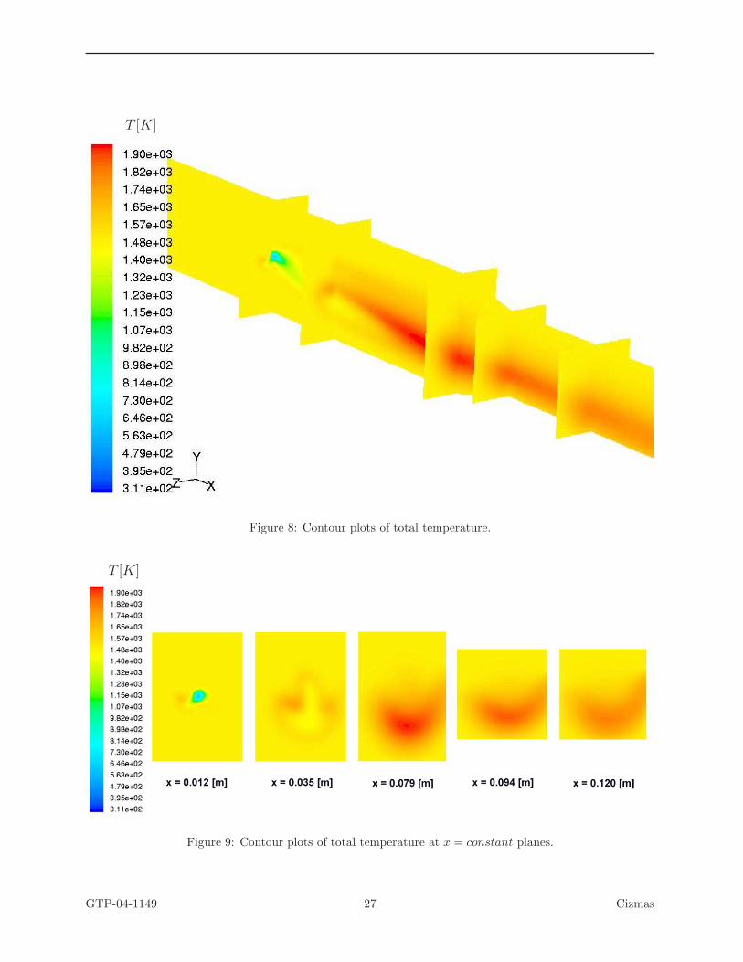
Figure 8 shows the variation of total temperature along the z=0 plane of the combustor and at five planes
perpendicular to the x-axis located at 12, 35, 79, 94 and 120 mm downstream of the injector. The maximum
total temperature was approximately 1970 K. Figure 9 shows total temperature variation in the five planes
described above. The total temperature predicted by the numerical simulation along the centerline at 836
mm downstream of the injector was 1602 K. The measured total temperature at the same location was 1544
K. The predicted temperature was 58 K higher than the measured temperature. There are several possible
reasons for the temperature difference, such as: (1) simplified kinetics scheme, (2) limitations of the k-ǫ
turbulence model, (3) approximations due to using binary diffusion coefficients, and (4) adiabatic boundary
conditions used in the simulation neglected the wall surface heat transfer that occurred in the experiment.
To improve temperature prediction, the combustion model was extended to include the backward reaction
of the carbon monoxide oxidation. The rate of the backward reaction of the CO/CO2 equilibrium was:
q2b = A2b exp (−E2/R/T ) [CO2] (5)
with A2b = 5 · 108(
m3/kmol)0.75
s−1 and E2/R = 20130 K. The total temperature predicted with this
improved kinetics model along the centerline, at 836 mm downstream of the injector, was 1562 K. Conse-
quently, the temperature difference between the experimental results and the numerical results was reduced
to 18 K. Note that the modeling of the backward reaction did not require solving for additional species, and
as a result the increase of the computational time was insignificant.
The accuracy of numerical prediction could also be increased by improving turbulence modeling. The
standard k-ǫ model used herein produced better results than the renormalization group or the realizable
k-ǫ models [35]. It has been reported that either the standard k-ω or the shear stress transport k-ω model
produced slightly better results than the k-ǫ model, without requiring additional computational time [36].
The Reynolds-stress turbulence model would probably produce more accurate results than the k-ǫ model,
but with a higher computational cost. However, the overall agreement between the measurements and the
predictions obtained with both the k-ǫ and Reynolds-stress turbulence models are reasonably good [37].
Regardless of the turbulence model used, the uncertainty caused by turbulence modeling grows as the
distance downstream of the flame increases.
GTP-04-1149 12 Cizmas
Gas chromatograph measurements at 0.311 m downstream of the injector found that the volume frac-
tion of CH4 was 0.35% and the volume fraction of CO was 0.16%. At the same location, the numerical
simulation predicted values close to zero (smaller than 10−4%) for methane. The carbon monoxide volume
fraction predicted by the chemical model (2) was 3 ·10−4% while the model that included the backward re-
action predicted 0.69%. This discrepancy between the numerical and experimental results indicates that the
methane oxidation happened more rapidly in the simulation than in the experiment. The species prediction
can be improved by using a reduced chemical kinetics model that includes more reactions [38, 39, 40]. The
computational cost of such a simulation, however, will increase several times, depending on the additional
number of species modeled. Since the purpose of this simulation was the prediction of the influence of
heat release on turbine-combustor performance, as opposed to predicting the detailed composition of the
combustion products, the two-reaction model was adopted herein.
The numerical simulation was done on an IBM Regatta pSeries 690 computer using 4 processors. The
computation converged in approximately 3,500 iterations. The wall clock time for this run was approximately
195 hours.
Four-Stage Turbine-Burner
Once the combustion model was tested for the single-vane burner, the next step was to investigate a four-stage
turbine-burner. The purpose of this numerical investigation was to determine the influence of several fuel
injection parameters on the unsteady flow and combustion in the turbine-burner. Since the computational
time of a three-dimensional model for the four-stage turbine-burner would exceed the computational time
of the single-vane burner by a factor of four, and since a parametric analysis of the turbine-burner was
necessary, it was decided to replace the three-dimensional model by a less computational expensive quasi-
three-dimensional model. A quasi-three-dimensional, as opposed to a two-dimensional model, was needed in
order to take into account the large radial variation of the four-stage turbine. Since Fluent did not have a
quasi-three-dimensional model, the CoRSI code was used instead.
GTP-04-1149 13 Cizmas

Geometry and Flow Conditions
The blade count of the four-stage turbine-combustor required a full-annulus simulation for a dimensionally
accurate computation. To reduce the computational effort, it was assumed that there were an equal number
of airfoils in each turbine row. As a result, all airfoils except for the inlet guide vane airfoils were rescaled by
factors equal to the number of airfoils per row divided by the number of airfoils of row one. An investigation
of the influence of airfoil count on the turbine flow showed that the unsteady effects were amplified when
a simplified airfoil count 1:1 was used [41]. Consequently, the results obtained using the simplified airfoil
count represent an upper limit for the unsteady effects.
The inlet temperature in the turbine-combustor exceeded 1800 K and the inlet Mach number was 0.155.
The inlet flow angle was 0 degrees and the inlet Reynolds number was 7,640,000 per meter, based on the
axial chord of the first-stage stator. The values of the species mass fractions at inlet in the turbine-burner
were: yCO2= 0.0775, yH2O = 0.068, yCO = 5.98 · 10−06, yH2
= 2.53 · 10−07, yO2= 0.1131, yN2
= 0.7288
and yAr = 0.0125. The rotational speed of the test turbine-burner was 3600 RPM.
The effects of in situ reheat were investigated by comparing the performances of a turbine-combustor for
several cases of fuel injection against the performance of the same turbine without combustion. Three of the
most representative cases are presented herein. Pure methane was injected at the trailing edge of the first
vane in all the cases of in situ reheat presented herein. The parameters that varied in the turbine-combustor
were the injection velocity, methane temperature and injection slot dimension. These parameters and the
fuel mass flow rate per vane and span length are presented in Table 2.
Table 2: Parameters of fuel injection.
Parameter Case 1 Case 2 Case 3
Injection velocity [m/s] 270.6 270.6 77Pressure [bar] 14.88 14.88 14.88Temperature [K] 313 590 313Injection slot size [mm] 0.54 0.54 1.36Fuel mass flow rate [x10−4 kg/s/vane/mm] 13.5 7.2 9.6
GTP-04-1149 14 Cizmas

Accuracy of Numerical Results
To validate the accuracy of the numerical results corresponding to the governing equations used, it was
necessary to show that the results were independent of the grid which discretizes the computational domain.
The verification of grid independence results was presented in [20], where a one-stage turbine-combustor was
simulated. Note that the grids were generated such that, for the given flow conditions, the y+ number was
less than 1. Approximately 20 grid points were used to discretize the boundary layer regions.
Based on the conclusions of accuracy investigation presented in [20], the medium grid was used herein
since it provided the best compromise between accuracy and computational cost. This grid had 53 grid
points normal to the airfoil and 225 grid points along the airfoil in the O-grid, and 75 grid points in the
axial direction and 75 grid points in the circumferential direction in the H-grid. The stator airfoils and rotor
airfoils had the same number of grid points. The inlet and outlet H-grids each had 36 grid points in the
axial direction and 75 grid points in the circumferential direction. The grid is shown in Fig. 10, where for
clarity every other grid point in each direction is shown.
The results presented in this paper were computed using three Newton sub-iterations per time-step and
2700 time-steps per cycle. Here, a cycle is defined as the time required for a rotor to travel a distance equal
to the pitch length at midspan. To ensure time-periodicity, each simulation was run in excess of 80 cycles.
The numerical simulation was done on a 64-processor SGI Origin 3800 computer. The computational time
for a run was approximately 160 hours.
Unsteady Temperature Variation
The variation of total enthalpy for the three in situ reheat cases and for the no combustion case is shown
in Fig. 11. The abscissa indicates the axial location. S1 denotes stator 1, R1 denotes rotor 1, etc. The
total enthalpy was calculated at the inlet and outlet of each row. Depending on the row type, that is, stator
or rotor, the total enthalpy was calculated using either the absolute or the relative velocity. The switch
between using absolute or relative velocities generated discontinuities between rows. As shown in Fig. 11, for
all fuel injection cases the total enthalpy increased compared to the no combustion case. The largest enthalpy
increase was located on the first rotor, where most of the combustion takes place. The combustion and heat
GTP-04-1149 15 Cizmas

release continued throughout the second stator and rotor, as indicated by the total enthalpy variation shown
in Fig. 11 [42].
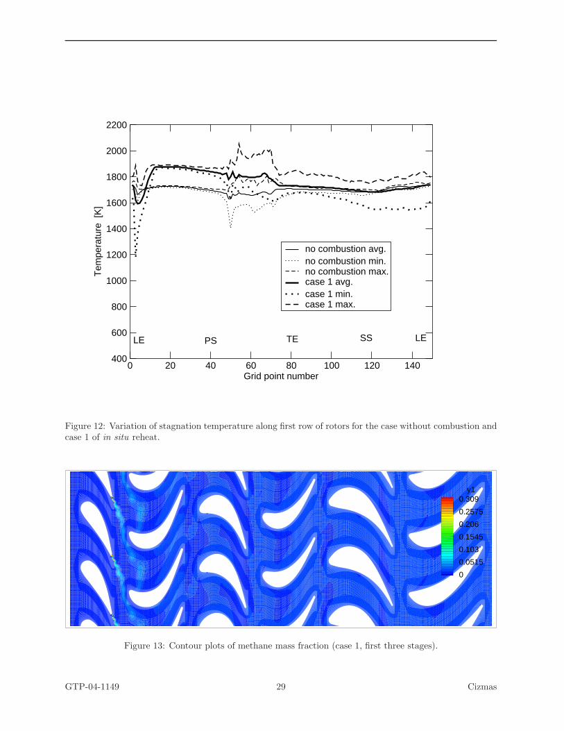
The stagnation temperature variation along the first row of rotors was strongly influenced by the in situ
reheat, as shown in Fig. 12. Figure 12 shows the averaged, minimum and maximum stagnation temperature
for the flow without combustion and for case 1 of flow with combustion. On the pressure side, the averaged
temperature of case 1 was approximately 180 K larger than the no combustion case temperature. At the
leading edge, however, the averaged temperature of case 1 was approximately 70 K lower than in the no
combustion case. On the suction side, the averaged temperature of case 1 was slightly higher than in the no
combustion case. On most of the suction side, the averaged temperature of case 1 was approximately 15 to
20 K larger than the no combustion case temperature.
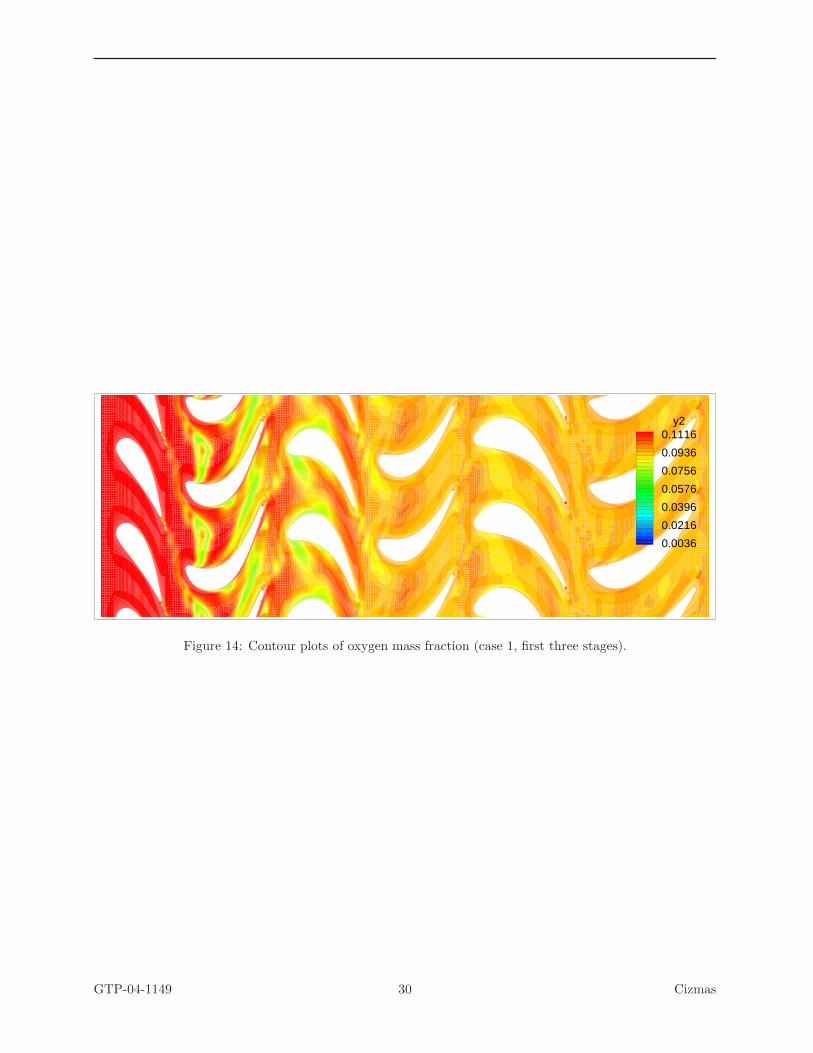
The averaged temperature indicates that combustion took place on the pressure side of the rotor airfoil.
This conclusion is also supported by snapshots of contour plots of methane and oxygen mass fraction shown in
Figs. 13 and 14. The existence of small regions where the averaged temperature of the case with combustion
was lower than the average temperature of the case without combustion indicates that combustion was
not completed. Consequently, the low enthalpy of the fuel injected reduced the airfoil temperature locally.
The maximum temperature of the case with combustion was larger than the maximum temperature of the
no combustion case over the entire airfoil. On the pressure side, the minimum temperature of the case
with combustion was larger than the minimum temperature of the case without combustion. On most of the
suction side, however, the minimum temperature of the case with combustion was smaller than the minimum
temperature of the case without combustion, indicating that the unburned, cold fuel injected was affecting
this region [42].
Unsteady Force Variation
The fuel injection in the turbine-combustor modified the tangential forces in the turbine, as shown in Table 3.
In situ reheat decreased tangential force Fy on the first blade row but increased tangential force on the
subsequent rows. Since the tangential force decrease on the first stage was smaller than the increase on the
subsequent stages, the power of the turbine-combustor increased for all cases with combustion. The largest
GTP-04-1149 16 Cizmas

power increase was 5.1% and corresponded to case 1. Power increased by 2.8% in case 2 and 4.6% in case
3. Although the variation of the averaged blade force Ftot was rather small, as shown in Table 3, the power
increase was significant.
Table 3: Forces on bladesNo Combustion Case 1 Case 2 Case 3
Ftot1 [kN] 18.28 18.21 18.71 18.67α1 [deg] 38.4 36.4 36.1 36.3Fy1 [kN] 11.36 10.81 11.03 11.05Ftot2 [kN] 11.87 12.27 12.17 12.31α2 [deg] 60.3 61.7 61.9 62.7Fy2 [kN] 10.31 10.81 10.74 10.94Ftot3 [kN] 12.62 13.19 12.75 13.08α3 [deg] 62.2 65.0 63.9 63.8Fy3 [kN] 11.17 11.95 11.45 11.73Ftot4 [kN] 11.41 13.03 12.31 12.58α4 [deg] 65.5 65.5 65.7 66.1Fy4 [kN] 10.38 11.85 11.21 11.51
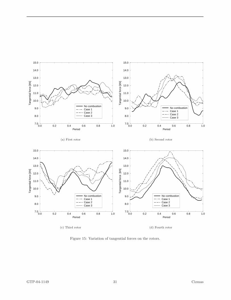
The time variation of the rotor blade tangential forces, shown in Fig. 15, indicates that the largest
amplitudes occurred in the last rotor row and the smallest amplitudes occurred in the first rotor row. This
conclusion is valid for every combustion or no combustion case.
A phase shift caused by fuel injection is visible for the first and second rotor blades. The larger unsteadi-
ness within the second rotor makes this phenomenon more clearly distinguishable in Fig. 15(b). The patches
of burning mixture and the reduced degree of mixedness were the probable causes for this tangential force
phase shift in the upstream region.
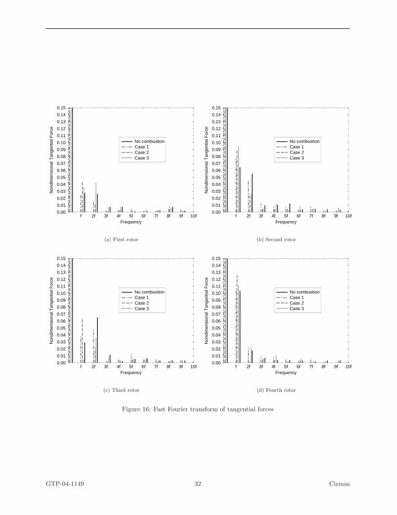
Figure 16 shows the fast Fourier transform of the tangential forces. They have been nondimensionalized
by the average tangential force obtained from the case without fuel injection. The blades of the fourth rotor
were excited the most. This excitation occurred at the first blade passing frequency (BPF), which was 1920
Hz. For the rest of the blades, the excitation due to the second BPF was comparable in amplitude to the
excitation of the first BPF. Except for the first rotor in case 1 and the third rotor in case 3, the fuel injection
increased the excitation of the first BPF. The largest amplitude increase was 216% and occurred on the
third-row blades in case 2. The unsteady force, however, was approximately 50% of the maximum amplitude
value that occurred on the fourth rotor blade at BPF [42].
GTP-04-1149 17 Cizmas
Conclusions
A two-reaction, global, finite rate combustion model was evaluated against experimental data for a single-
vane burner. This combustion model has been utilized to explore the effects of in situ reheat in a four-
stage turbine-combustor. The complexity of the transport phenomena in a multi-stage turbine-combustor
generated a challenging numerical simulation. The large unsteadiness and straining of the flow along with
the wide range of velocity variation lead to a wide range of local characteristic time scales for flow and
combustion, which strongly impacted the on-going reactions.
The numerical simulation was used to predict the airfoil temperature variation and the unsteady blade
loading in a four-stage turbine-combustor. The largest excitation of the four-stage turbine-combustor corre-
sponded to the fourth-stage rotor, with or without combustion. The highest excitation corresponded to the
first blade passing frequency, for all cases analyzed.
The in situ reheat decreased the power of the first stage, but increased more the power of the following
stages. The power of the turbine increased between 2.8% and 5.1%, depending on the parameters of the fuel
injection.
Acknowledgments
This paper was prepared with the support of the U. S. Department of Energy (DOE), under Award No. DE-
FC26-00NT40913. However, any opinions, findings, conclusions, or recommendations expressed herein are
those of the authors and do not necessarily reflect the views of the DOE. The Government reserves for itself
and others acting on its behalf a royalty-free, nonexclusive, irrevocable, worldwide license for Governmental
purposes to publish, distribute, translate, duplicate, exhibit and perform this copyrighted paper. Additional
funding was provided by Siemens Westinghouse Power Corporation. The authors gratefully acknowledge the
support of Mr. Charles Alsup, the DOE project manager. The authors also appreciate the support of the
Texas A&M Supercomputing Center and the Super-Computing Science Consortium (SC)2 who generously
provided access to the computing resources of the Pittsburgh Supercomputing Center.
GTP-04-1149 18 Cizmas

Nomenclature
A Arrhenius factor
E Activation energy
e Total intrinsic internal energy per unit volume
(F, G) Inviscid flux vector in curvilinear coordinates
(f, g) Inviscid flux vector in Cartesian coordinates
M Mach number
M Molar mass
Nr Number of reactions
p Pressure
Q State vector in curvilinear coordinates
q State vector in Cartesian coordinates or rate of progress
R Universal gas constant
Re Reynolds number
S Viscous flux vector
u Fluid velocity in the x-direction
v Fluid velocity in the y-direction
yi Mass fraction of species i
w Species net production rate
γ Adiabatic exponent (Ratio of specific heats)
ν Stoichiometric coefficient
ρ Density
τ Non-dimensional time
(ξ, η) Curvilinear coordinates
GTP-04-1149 19 Cizmas

Subscripts
ch Chemical source term
i Species index
∞ Upstream infinity
Superscripts
ns Navier-Stokes
sp Species
′′ products
′ reactants
References
[1] Sirignano, W. A., and Liu, F., 1999. “Performance increases for gas-turbine engines through combustion
inside the turbine”. Journal of Propulsion and Power, 15 (1) , pp. 111–118.
[2] Simpson, J. R., and May, G. C., 1964. Reheat apparatus for a gas turbine engine. Unites States Patent
Office: 3,141,298, Rolls-Royce Limited, Derby, England, July.
[3] Witt, S. H. D., 1967. Reheat gas turbine power plant with air admission to the primary combustion
zone of the reheat combustion chamber structure. Unites States Patent Office: 3,315,467, Westinghouse
Electric Corporation, Pittsburgh, Pennsylvania, April.
[4] Althaus, R., Farkas, F., Graf, P., Hausermann, F., and Kreis, E., 1995. Method of operating gas turbine
group with reheat combustor. Unites States Patent Office: 5,454,220, Asea-Brown-Boveri, Baden,
Switzerland, October.
[5] Dills, R. R., and Follansbee, P. S., 1979. Use of thermocouples for gas temperature measurements in a
gas turbine combustor. Tech. rep., National Bureau of Standards, October. Special Publication 561.
[6] Elmore, D. L., Robinson, W. W., and Watkins, W. B., 1983. Dynamic gas temperature measurement
system. Tech. rep., NASA, May. Contractor Report 168267.
GTP-04-1149 20 Cizmas
[7] Butler, T. L., Sharma, O. P., Joslyn, H. D., and Dring, R. P., 1989. “Redistribution of an inlet
temperature distortion in an axial flow turbine stage”. Journal of Propulsion and Power, 5 January-
February , pp. 64–71.
[8] Graham, R. W., 1980. “Fundamental mechanisms that influence the estimate of heat transfer to gas
turbine blades”. Heat Transfer Engineering, 2 (1) July-September , pp. 39–47.
[9] Kirtley, K. R., Celestina, M. L., and Adamczyk, J. J., 1993. “The effect of unsteadiness on the time-mean
thermal loads in a turbine stage”. SAE Paper 931375.
[10] Whitney, W. J., Stabe, R. G., and Moffitt, T. P., 1980. Description of the warm core turbine facility
and the warm annular cascade facility recently installed at NASA Lewis Research Center. Tech. rep.,
NASA. Technical Memorandum 81562.
[11] Schwab, J. R., Stabe, R. G., and Whitney, W. J., 1983. “Analytical and experimental study of
flow through and axial turbine stage with a nonuniform inlet radial temperature profile”. In 19th
AIAA/SAE/ASME Joint Propulsion Conference, AIAA Paper 83-1175.
[12] Stabe, R. G., Whitney, W. J., and Moffitt, T. P., 1984. “Performance of a high-work low aspect
ratio turbine tested with a realistic inlet radial temperature profile”. In 20th AIAA/SAE/ASME Joint
Propulsion Conference, AIAA Paper 84-1161.
[13] Sharma, O. P., Pickett, G. F., and Ni, R. H., 1992. “Assessment of unsteady flows in turbomachines”.
Journal of Turbomachinery, 114 (1) January , pp. 79–90.
[14] Shang, T., Guenett, G. R., Epstein, A. H., and Saxer, A. P., 1995. “The influence of inlet temperature
distortion on rotor heat transfer in a transonic turbine”. In 31st AIAA/ASME/SAE/ASEE Joint
Propulsion Conference, AIAA Paper 95-3042.
[15] Rai, M. M., and Dring, R. P., 1990. “Navier-Stokes analyses of the redistribution of inlet temperature
distortions in a turbine”. Journal of Propulsion and Power, 6 (3) , pp. 276–282.
[16] Krouthen, B., and Giles, M. B., 1988. “Numerical investigation of hot streaks in turbines”. In 24th
AIAA/SAE/ASME/ASEE Joint Propulsion Conference, AIAA Paper 88-3015.
GTP-04-1149 21 Cizmas
[17] Takahashi, R. K., and Ni, R. H., 1991. “Unsteady hot streak migration through a 1-1/2 stage turbine”.
In 27th AIAA/SAE/ASME/ASEE Joint Propulsion Conference, AIAA Paper 91-3382.
[18] Shang, T., and Epstein, A. H., 1996. “Analysis of hot streak effects on turbine rotor heat load”. In
International Gas Turbine and Aeroengine Congress, ASME Paper 96-GT-118.
[19] Dorney, D. J., Sondak, D. L., and Cizmas, P. G. A., 2000. “Effects of hot streak/airfoil ratios in a high-
subsonic single-stage turbine”. International Journal of Turbo and Jet Engines, 17 (2) , pp. 119–132.
[20] Isvoranu, D. D., and Cizmas, P. G. A., 2003. “Numerical simulation of combustion and rotor-stator
interaction in a turbine combustor”. International Journal of Rotating Machinery, 9 (5) , pp. 363–374.
[21] Balakrishnan, A., 1987. “Application of a flux-split algorithm to chemically relaxing, hypervelocity
blunt-body flows”. In 22nd Thermophysics Conference, AIAA Paper 87-1578, AIAA.
[22] Cizmas, P., Flitan, H., and Isvoranu, D., 2003. “Numerical prediction of unsteady blade loading in
a turbine-combustor”. In 8th National Turbine High Cycle Fatigue Conference. Universal Technology
Corporation, Monterey, CA, April.
[23] Westbrook, C. K., and Dryer, F. L., 1981. “Simplified reaction mechanisms for the oxidation of hydro-
carbon fuels in flames”. Combustion Science and Technology, 27 , pp. 31–43.
[24] Hautman, J., Dryer, F. L., Schug, K. P., and Glassman, I., 1981. “A multiple-step overall kinetic
mechanism for the oxidation of hydrocarbons”. Combustion Science and Technology, 25 , pp. 219–235.
[25] Cizmas, P. G. A., and Subramanya, R., 1997. “Parallel computation of rotor-stator interaction”. In
The Eight International Symposium on Unsteady Aerodynamics and Aeroelasticity of Turbomachines,
T. H. Fransson, Ed., pp. 633–643.
[26] Roe, P. L., 1981. “Approximate Riemann solvers, parameter vectors, and difference schemes”. Journal
of Computational Physics, 43 , pp. 357–372.
[27] Eberhardt, S., and Brown, K., 1986. “A shock capturing technique for hypersonic, chemically relaxing
flows”. In 24th Aerospace Sciences Meeting, AIAA Paper 86-0231, AIAA.
GTP-04-1149 22 Cizmas

[28] Yee, H. C., 1987. “Construction of explicit and implicit symmetric schemes and their applications”.
Journal of Computational Physics, 68 , pp. 151–179.
[29] Li, C. P., 1987. “Chemistry-split techniques for viscous reactive blunt body flow computations”. In
25th Aerospace Sciences Meeting, AIAA Paper 87-0282, AIAA.
[30] Warming, R. F., and Beam, R. M., 1978. “On the construction and application of implicit factored
schemes for conservation laws”. SIAM-AMS Proceedings, 11 , pp. 85–129.
[31] Rai, M. M., and Chakravarthy, S., 1986. “An implicit form for the Osher upwind scheme”. AIAA
Journal, 24 , pp. 735–743.
[32] Rai, M. M., 1985. “Navier-Stokes simulation of rotor-stator interaction using patched and overlaid
grids”. In AIAA 7th Computational Fluid Dynamics Conference, AIAA Paper 85-1519.
[33] Fluent Inc., 2002. Gambit 2.0: Training Notes, January.
[34] Fluent Inc., 2003. Fluent 6.1: Training Notes, March.
[35] Christo, F., and Dally, B., 2005. “Modeling turbulent reacting jets issuing into a hot and diluted coflow”.
Combustion and Flame, 142 , pp. 117–129.
[36] Engdar, U., Nilsson, P., and Klingmann, J., 2004. “Investigation of turbulence models applied to
premixed combustion using a level-set flamelet library approach”. Journal of Engineering for Gas
Turbine and Power, 126 , pp. 701–707.
[37] German, A., and Mahmud, T., 2005. “Modelling of non-premixed swirl burner flows using a reynolds-
stress turbulence closure”. Fuel, 84 , pp. 583–594.
[38] Nicol, D. G., Malte, P. C., Hamer, A. J., Roby, R. J., and Steele, R. C., 1999. “Development of a
five-step global methane oxidation - no formation mechanism for lean-premixed gas turbine”. Journal
of Engineering for Gas Turbines and Power - Transactions of the ASME, 121 (2) , pp. 272–280.
[39] Sung, C. J., Law, C. K., and Chen, J.-Y., 2001. “Augmented reduced mechanisms for NO emission in
methane oxidation”. Combustion and Flame, 125 , pp. 906–919.
GTP-04-1149 23 Cizmas
[40] Barlow, R. S., 2003. International workshop on measurement and computation of turbulent nonpremixed
flames. http://www.ca.sandia.gov/TNF. Sandia National Laboratories.
[41] Cizmas, P. G. A., 1999. Transition and blade count influence on steam turbine clocking. Tech. rep.,
Texas Engineering Experiment Station, College Station, Texas, January.
[42] Flitan, H. C., and Cizmas, P. G. A., 2003. “Analysis of unsteady aerothermodynamics effects in a turbine
combustor”. In The Tenth International Symposium on Unsteady Aerodynamics and Aeroelasticity of
Turbomachines. Durham, North Carolina, September.
GTP-04-1149 24 Cizmas

YCH4
Figure 4: Contour plots of methane mass fraction.
YCH4
Figure 5: Contour plots of methane mass fraction at x = constant planes.
GTP-04-1149 25 Cizmas
YCO
Figure 6: Contour plots of carbon monoxide mass fraction.
YCO
Figure 7: Contour plots of carbon monoxide mass fraction at x = constant planes.
GTP-04-1149 26 Cizmas
T [K]
Figure 8: Contour plots of total temperature.
T [K]
Figure 9: Contour plots of total temperature at x = constant planes.
GTP-04-1149 27 Cizmas

Figure 10: Detail of the medium grid (every other grid point in each direction shown).
1 2 3 4 5 6 7 8 9Station
1000
1500
2000
2500
3000
3500
4000
Tot
al e
ntha
lpy
[kJ/
kg]
no combustioncase 1case 2case 3
S1 R1 S2 R2 S3 R3 S4 R4
Figure 11: Variation of averaged total enthalpy (absolute or relative).
GTP-04-1149 28 Cizmas
0 20 40 60 80 100 120 140Grid point number
400
600
800
1000
1200
1400
1600
1800
2000
2200
Tem
pera
ture
[K
]
no combustion avg.no combustion min.no combustion max.case 1 avg.case 1 min.case 1 max.
LE TE LEPS SS
Figure 12: Variation of stagnation temperature along first row of rotors for the case without combustion andcase 1 of in situ reheat.
y10.309
0.2575
0.206
0.1545
0.103
0.0515
0
Figure 13: Contour plots of methane mass fraction (case 1, first three stages).
GTP-04-1149 29 Cizmas
y20.1116
0.0936
0.0756
0.0576
0.0396
0.0216
0.0036
Figure 14: Contour plots of oxygen mass fraction (case 1, first three stages).
GTP-04-1149 30 Cizmas
0.0 0.2 0.4 0.6 0.8 1.0Period
7.0
8.0
9.0
10.0
11.0
12.0
13.0
14.0
15.0
Tan
gent
ial f
orce
[kN
]
No combustionCase 1Case 2Case 3
(a) First rotor
0.0 0.2 0.4 0.6 0.8 1.0Period
7.0
8.0
9.0
10.0
11.0
12.0
13.0
14.0
15.0
Tan
gent
ial f
orce
[kN
]
No combustionCase 1Case 2Case 3
(b) Second rotor
0.0 0.2 0.4 0.6 0.8 1.0Period
7.0
8.0
9.0
10.0
11.0
12.0
13.0
14.0
15.0
Tan
gent
ial f
orce
[kN
]
No combustionCase 1Case 2Case 3
(c) Third rotor
0.0 0.2 0.4 0.6 0.8 1.0Period
7.0
8.0
9.0
10.0
11.0
12.0
13.0
14.0
15.0
Tan
gent
ial f
orce
[kN
]
No combustionCase 1Case 2Case 3
(d) Fourth rotor
Figure 15: Variation of tangential forces on the rotors.
GTP-04-1149 31 Cizmas
f 2f 3f 4f 5f 6f 7f 8f 9f 10fFrequency
0.00
0.01
0.02
0.03
0.04
0.05
0.06
0.07
0.08
0.09
0.10
0.11
0.12
0.13
0.14
0.15
Non
dim
ensi
onal
Tan
gent
ial F
orce
No combustionCase 1Case 2Case 3
(a) First rotor
f 2f 3f 4f 5f 6f 7f 8f 9f 10fFrequency
0.00
0.01
0.02
0.03
0.04
0.05
0.06
0.07
0.08
0.09
0.10
0.11
0.12
0.13
0.14
0.15
Non
dim
ensi
onal
Tan
gent
ial F
orce
No combustionCase 1Case 2Case 3
(b) Second rotor
f 2f 3f 4f 5f 6f 7f 8f 9f 10fFrequency
0.00
0.01
0.02
0.03
0.04
0.05
0.06
0.07
0.08
0.09
0.10
0.11
0.12
0.13
0.14
0.15
Non
dim
ensi
onal
Tan
gent
ial F
orce
No combustionCase 1Case 2Case 3
(c) Third rotor
f 2f 3f 4f 5f 6f 7f 8f 9f 10fFrequency
0.00
0.01
0.02
0.03
0.04
0.05
0.06
0.07
0.08
0.09
0.10
0.11
0.12
0.13
0.14
0.15
Non
dim
ensi
onal
Tan
gent
ial F
orce
No combustionCase 1Case 2Case 3
(d) Fourth rotor
Figure 16: Fast Fourier transform of tangential forces
GTP-04-1149 32 Cizmas


![Horia Matei - Maiasii [Gray]](https://cdn.vdocuments.net/doc/165x107/5695d4c71a28ab9b02a2be5b/horia-matei-maiasii-gray.jpg)


