System-Level Design Decision-Making for Real-Time Embedded Systems
PROEFSCHRIFT
ter verkrijging van de graad van doctor aan de Technische Universiteit Eindhoven, op gezag van de
Rector Magnificus, prof.dr. R.A. van Santen, voor een commissie aangewezen door het College voor
Promoties in het openbaar te verdedigen op dinsdag 14 december 2004 om 16.00 uur
door
Sien-An Ong
geboren te Sungailiat, Indonesië
ii
Dit proefschrift is goedgekeurd door de promotoren: prof.ir. M.P.J. Stevens en prof.dr.ir. R.H.J.M. Otten Copromotor: dr.ir. L. Jóźwiak
© Copyright 2004 S.A. Ong
All rights reserved. No part of this publication may be reproduced, stored in a retrieval system, or transmitted, in any form or by any means, electronic, mechanical, photocopying, recording, or otherwise, without the prior written permission from the copyright owner. Printed by: Universiteitsdrukkerij Technische Universiteit Eindhoven CIP-DATA LIBRARY TECHNISCHE UNIVERSITEIT EINDOVEN
Ong, Sien An
System-level design decision-making for real-time embedded systems / by Sien-An Ong.- Eindhoven : Technische Universiteit Eindhoven, 2004.
Proefschrift. -ISBN 90-386-1002-5
NUR 959
Trefw: ingebedde systemen / systeemanalyse / beslissingstheorie / genetische algoritmen / microprocessoren ; real-time systemen / geintegreerde schakelingen ; ontwerp
Subject headings: embedded systems / systems analysis / decision making / operations research / genetic algorithms / CAD

iii

iv

v
System-Level Design Decision-Making for Real-Time Embedded Systems

vi
vii
SUMMARY
As the size and complexity of real-time embedded systems increase, the specification
and design of the overall system architecture is becoming ever more important. In order to
be able to make the right system architecture selection, the feasibility of candidate
functional behavior - hardware architecture pairs need to be predicted already at the early
stages of design.
The applications considered in this thesis are real-time embedded systems that have a
mix of control and data-flow functionality, and are implemented as mixed
hardware/software systems. The real-time embedded systems considered belong to a
relatively limited, well-defined, well-known, analyzed and characterized system class, so
that a certain general solution form (generic architecture template) is known for the systems,
and a particular system architecture for a particular system of this class can be obtained by a
certain instantiation of this general form. However, the class of the considered systems is
not so much limited and not so well known, that a parameterized architecture generator can
be built. In order to predict the feasibility of a particular system, the mapping and
scheduling must be constructed in the light of the system parametric constraints, objectives
and trade-off information.
The feasibility analysis is organized as a heuristic search. During such heuristic search
some promising instantiations of the generic architecture form are proposed, analyzed,
estimated and selected, and mapping of the network of the system processes on the network
of the system structural modules must be performed. The analysis involves the creation of a
model, which characterizes the functional behavior of the system and facilitates behavioral
analysis, the construction of the modeling constructs that defines the decision space for the
mapping and scheduling problem, and the construction of the heuristic search that is
organized as a genetic algorithm equipped with multi-criteria decision-making aids for
predicting the feasibility of the candidate functional behavior – hardware architecture pairs.
In this work, some new opportunities and difficulties related to the system-on-a-chip
technology are overviewed, the nature of the complex system design problems is analyzed
and an appropriate quality-driven system design methodology is proposed and discussed.

viii

ix
SAMENVATTING
Met de toename aan grootte en complexiteit van real-time embedded systems, wordt het
te uiteindelijk ontworpen systeem in steeds grotere mate door de systeemarchitectuur
bepaald. Om vroeg in het design traject de juiste systeemarchitectuur te kunnen selecteren,
moet men in staat zijn om de uitvoerbaarheid van bepaalde functionaliteit en hardware
architectuur combinaties al in deze fase te toetsen.
In het proefschrift worden real-time embedded systemen applicaties die een mix van
control en data-flow functies bezitten en een hardware/software systeem implementatie
hebben besproken. De systemen behoren tot een relatief beperkt, goed gedefinieerde klas
van systemen, met betrekkelijk bekende eigenschappen. Dit maakt een algemene oplossing
(hardware architectuur template) mogelijk. Een systeem oplossing is dan een instantiatie
van de algemene oplossing. De oplossingsruimte is echter nog zodanig groot en onbekend
dat een architectuur generator waarvoor slechts de parameters ingesteld dienen te worden,
niet mogelijk is. Om de uitvoerbaarheid te toetsen worden de toewijzing en tijdsplanning
van een systeem daarom berekend, waarbij doelstellingen dienen te worden nagestreefd, en
rekening te worden gehouden met de systeem beperkingen en afwegingen van de systeem
architect.
De uitvoerbaarheidanalyse is opgezet als een heuristiek zoek proces, waarbij
tussenoplossingen met een mogelijk hoog potentieel worden gegenereerd, geanalyseerd,
getoetst en eventueel geselecteerd. De uitvoerbaarheidanalyse omvat het modelleren van het
functionele gedrag, de constructie van modelleringconstructen welke de toegestane
beslissingsruimte definieert, en de ontwikkeling van de zoek heuristiek voor het oplossen
van het toewijzing and tijdsplanning probleem. De heuristiek maakt gebruik van genetische
algoritmen en multi-criteria decision-making methoden.
In het proefschrift wordt een overzicht gegeven van de mogelijkheden en problemen van
system-on-chip technologie. De problemen bij het ontwerpen van complexe systemen
worden geanalyseerd en een voorstel voor een passend kwaliteitsgedreven systeem ontwerp
methode wordt gegeven en bediscussieerd.

x
xi
Contents
SUMMARY .................................................................................................................. VII
SAMENVATTING......................................................................................................... IX
CHAPTER 1. INTRODUCTION.............................................................................. 1
1.1 MOTIVATION...................................................................................................... 1
1.2 SCOPE OF THE SYSTEM-LEVEL DESIGN................................................... 2
1.3 APPLICATION-SPECIFIC REAL-TIME EMBEDDED SYSTEMS............. 4
1.4 RESEARCH SUBJECT........................................................................................ 6
1.5 PREVIOUS WORKS RELATED TO THE SUBJECT .................................... 9
1.6 PROBLEM STATEMENT AND RESEARCH AIMS .................................... 11
1.7 MAIN ASSUMPTIONS AND SOLUTION CONCEPTS ............................... 14
1.8 MAIN CONTRIBUTION AND OUTLINE OF WORK ................................. 25
CHAPTER 2. MODELING OF EMBEDDED SYSTEMS................................... 29
2.1 INTRODUCTION............................................................................................... 29
2.2 SASD METHOD ................................................................................................. 32
2.3 SA/RT MODELS................................................................................................. 34
2.4 LABELED TRANSITION SYSTEMS.............................................................. 41
2.5 LABELED NET SYSTEMS............................................................................... 45
2.6 CAUSAL NETS................................................................................................... 47
xii
2.7 NET SYSTEM OPERATORS............................................................................ 50
2.8 ABSTRACT COMMUNICATION ................................................................... 52
CHAPTER 3. DECISION-MAKING FOR SYSTEM DESIGN .......................... 57
3.1 INTRODUCTION ............................................................................................... 57
3.2 MCDM FOR QUALITY-DRIVEN DESIGN DECISION-MAKING............ 58
3.3 MCDM METHODS ............................................................................................ 60 3.3.1 Basic Notions ................................................................................................. 60 3.3.2 MCDM Model-Based Process ....................................................................... 63
3.4 MULTI-ATTRIBUTE DECISION-MAKING METHODS............................ 63 3.4.1 Utility Functions............................................................................................. 64 3.4.2 Aspiration-Based Methods............................................................................. 64 3.4.3 Outranking Methods....................................................................................... 66 3.4.4 Non-Compensatory Methods ......................................................................... 68
3.5 MULTI-OBJECTIVE OPTIMIZATION PROBLEMS.................................. 68
3.6 DECISION-MAKING FOR SYSTEM DESIGN ............................................. 70
3.7 GENETIC ALGORITHMS................................................................................ 72 3.7.1 Basic Principles .............................................................................................. 72 3.7.2 Crowding distance.......................................................................................... 76 3.7.3 Selection Operator.......................................................................................... 77 3.7.4 Post-processing .............................................................................................. 80
CHAPTER 4. BEHAVIORAL MODEL................................................................. 83
4.1 APPROXIMATE SYSTEM BEHAVIOR......................................................... 83 4.1.1 Data Transformation State Machines............................................................. 84 4.1.2 Control Transformation State Machines ........................................................ 86 4.1.3 Branches and Merges ..................................................................................... 86
4.2 TRANSITION SYSTEM REPRESENTATION .............................................. 87
4.3 MULTI-EVENT ABSTRACTION .................................................................... 92
4.4 BEHAVIORAL MODELING OF MULTI-EVENT TRANSITIONS ........... 94 4.4.1 Transition System Model ............................................................................... 94
xiii
CHAPTER 5. INTERNAL MODEL....................................................................... 97
5.1 INTRODUCTION............................................................................................... 97
5.2 LABELLED NET SYSTEM OPERATORS .................................................... 98
5.3 BEHAVIORAL MODELING OF MULTI-EVENT TRANSITIONS......... 100
5.4 SEQUENTIAL COMPONENTS..................................................................... 101 5.4.1 Covering....................................................................................................... 101 5.4.2 Contact-Freeness.......................................................................................... 103 5.4.3 Characterization of States and Actions........................................................ 103
5.5 MULTI-EVENT TRANSITION CONSTRUCTION .................................... 105 5.5.1 Multi-Event Transition Grouping ................................................................ 105 5.5.2 Resolving Conflicts between Multi-Event Transitions................................ 108
5.6 SOME CHARACTERISTICS OF THE COMPOSITE NET SYSTEM..... 110 5.6.1 Redundant Transitions ................................................................................. 110
5.7 EXAMPLE......................................................................................................... 110
CHAPTER 6. OPTIMIZATION MODEL........................................................... 123
6.1 INTRODUCTION............................................................................................. 123
6.2 BEHAVIORAL MODEL ................................................................................. 124 6.2.1 Task Graphs ................................................................................................. 124 6.2.2 Data Transfer ............................................................................................... 126
6.3 TARGET ARCHITECTURE MODEL .......................................................... 129
6.4 OPTIMIZATION MODEL.............................................................................. 134 6.4.1 Sub-model per use case................................................................................ 134 6.4.2 Sub-model per use case, and per kernel....................................................... 134 6.4.3 Mapping Configuration................................................................................ 135 6.4.4 Order of Multiple Runs................................................................................ 135 6.4.5 Placeholders for Transformation Runs ........................................................ 135
6.5 MODELING CONSTRUCTS FOR COSTS .................................................. 137 6.5.1 Costs Constraints ......................................................................................... 137 6.5.2 Transformation Run Delay .......................................................................... 139
6.6 MODELING CONSTRUCTS FOR LOCAL MEMORY USE .................... 141
xiv
6.6.1 Blocks, Stores and Data-flows ..................................................................... 141 6.6.2 Blocks........................................................................................................... 141 6.6.3 Functions and Variables for Blocks ............................................................. 142 6.6.4 Mutual Order of Blocks ............................................................................... 143 6.6.5 Initialization and Offloading Costs .............................................................. 145 6.6.6 Memory Allocation for Blocks .................................................................... 146 6.6.7 Stores and Data-flows .................................................................................. 147 6.6.8 Resource Allocation Schemes for Stores and Data-flows............................ 149
6.7 MODELING CONSTRUCTS FOR SCHEDULING ORDER ..................... 151 6.7.1 Precedence Constraints ................................................................................ 151 6.7.2 Main Memory Buffering Policy................................................................... 152
6.8 GENETIC REPRESENTATION OF INDIVIDUALS .................................. 153 6.8.1 Genetic Representation ................................................................................ 153
6.9 DECODING ALGORITHM ............................................................................ 154
6.10 SELECTION OPERATOR .......................................................................... 156 6.10.1 Enhanced Non-dominated Sorting ............................................................... 156 6.10.2 Imprecise Assessments................................................................................. 156
6.11 CROSSOVER AND MUTATION OPERATOR........................................ 158 6.11.1 Crossover of Total Order ............................................................................. 158 6.11.2 Crossover of Mapping Configurations......................................................... 159 6.11.3 Mutation of Total Order ............................................................................... 159 6.11.4 Mutation of Mapping Configuration............................................................ 160
6.12 CONSTRAINTS AND OBJECTIVES......................................................... 160
6.13 REPAIR ALGORITHM ............................................................................... 163
6.14 LOCAL FINE TUNING................................................................................ 164 6.14.1 Exploiting Sensitivity of Decision Variables ............................................... 164
CHAPTER 7. DESIGN CASES............................................................................. 167
7.1 BEHAVIORAL ANALYSIS............................................................................. 167
7.2 COST ESTIMATION ....................................................................................... 173
7.3 COST ESTIMATION OF DATA TRANSFORMATION ............................ 174
7.4 COST ESTIMATION METHOD FOR DATA PATHS................................ 175

xv
7.5 VIDEO ENCODER........................................................................................... 181
CHAPTER 8. CONCLUSIONS ............................................................................ 193
REFERENCES............................................................................................................. 199
APPENDIX A. NET SYSTEMS ................................................................................ 213
APPENDIX B. ADDITIONAL DESIGN CASE ...................................................... 217


1
Chapter 1.
Introduction
1.1 Motivation
The complexity of micro-electronics-based systems technologically feasible has
increased in a steady pace. Modern micro-electronic technology enables the
implementation of a complete complex information processing system on a single chip.
The designer's productivity has however not grown with the same pace resulting in a gap
between designer's productivity and complexity of systems technologically feasible. The
Sematech 2003 roadmap [130] estimates that a roughly 50× increase in design
productivity over what is possible today is required in order to exploit the enormous
system complexity that can be realized on a single die. In the meanwhile, there is a
strong customer demand for products with ever-increasing system complexity and
functionality. These trends can be carried back to the growth of the personal information
flow through the Internet, voice, and data communication devices, and are expected to
continue. Progress in micro-electronic technology is extremely fast and it is outstripping
the system designers' ability to make use of created opportunities. These developments
put much pressure on companies to exploit the potential chip complexity in an efficient
and effective manner. Disclaiming the trends most definitely means to loose ground to
competitors who act up to the trends emerging.
A source of the complexity is that systems are becoming more heterogeneous,
requiring a diversity of design styles, and diversity of implementation technologies.
Embedded systems (i.e. systems that are tightly integrated in another system) and
embedded software become key design issues [130]. These factors are leading to the
quality problems, delayed project schedules, and missed revenues. Assigning more

2
engineers to the project may not result in the desired outcome, since one big part of the
complexity growth relates to the problem of system integration. System complexity has
grown to a point out where individual designers cannot comprehend the detailed
functionality of the system anymore, using traditional design methods. A more sensible
approach compared to assigning more designers seems to be to raise the level of
abstraction at which systems are being designed to the system-level and increase the
quality and extent of adequate system-level design automation [130].
The design and production cost and time of the micro-electronics-based systems, as
well as their complexity and quality tend to be more limited by the design methods and
tools than by the micro-electronic technology [79] [107] [130]. Substantial improvement
can only be achieved through development and application of a new generation of more
suitable design paradigms, methods and tools. In this thesis, some new opportunities and
difficulties related to the system-on-a-chip technology are overviewed, the nature of the
complex system design problems is analyzed and an appropriate quality-driven system
design method is proposed and discussed.
1.2 Scope of the System-Level Design
As embedded systems implementation moves from digital microprocessors and
application-specific integrated circuits towards systems-on-a-chip technology, it is
necessary to consider the whole system in its entirety rather than the software and
hardware parts in isolation. Over the years, some agreement has been reached on the
levels of abstraction for hardware and software by using the principle of separation of
concerns. Each level describes different concerns that allow for different abstraction by
their consideration. The same principle should be applied when considering the system
as a whole and the interrelations between the hardware and software system modules.
The models used should be at a higher level of abstraction than those traditionally used
in design of hardware and/or software.
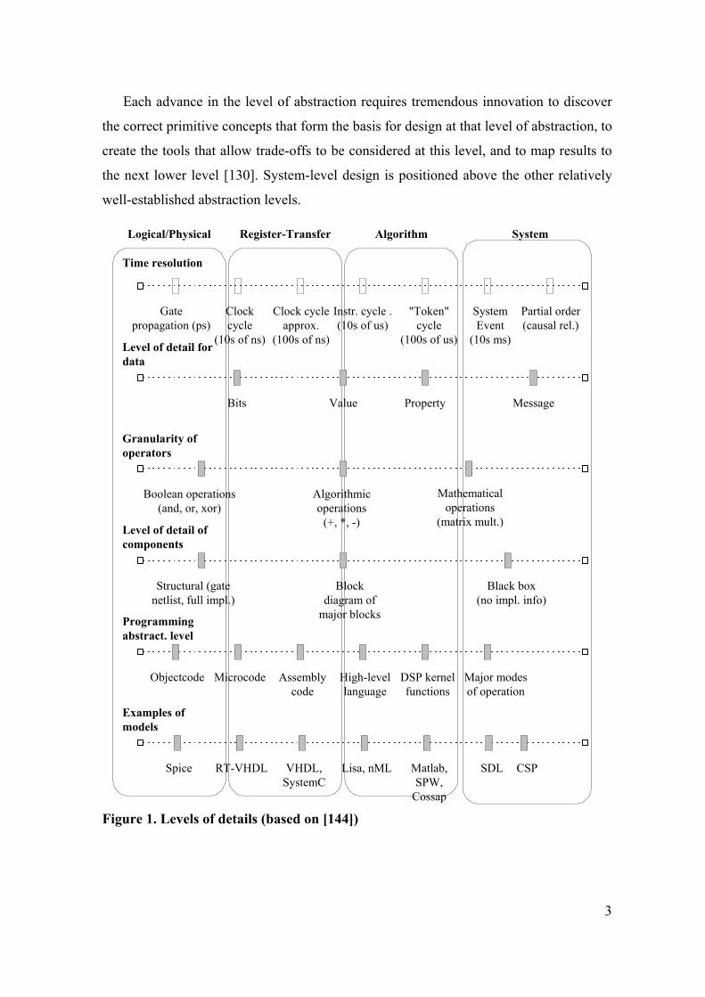
Coarsely, four levels of abstraction are being distinguished in the design of micro-
electronic-based systems: system-, algorithm-, register-transfer-, and logical-/physical-
level [144]. In order to grasp the scope of the system-level design, a description for the
levels of details is given in Figure 1. It is based on the taxonomy model of the VSIA
[144].
3
Each advance in the level of abstraction requires tremendous innovation to discover
the correct primitive concepts that form the basis for design at that level of abstraction, to
create the tools that allow trade-offs to be considered at this level, and to map results to
the next lower level [130]. System-level design is positioned above the other relatively
well-established abstraction levels.
Gatepropagation (ps)
Clockcycle
(10s of ns)
Clock cycleapprox.
(100s of ns)
Instr. cycle .(10s of us)
"Token"cycle
(100s of us)
SystemEvent
(10s ms)
Partial order(causal rel.)
Time resolution
PropertyBits Value Message
Level of detail fordata
Level of detail ofcomponents
Black box(no impl. info)
Structural (gatenetlist, full impl.)
Blockdiagram of
major blocks
Objectcode Microcode Assemblycode
High-levellanguage
DSP kernelfunctions
Major modesof operation
Programmingabstract. level
Spice RT-VHDL VHDL,SystemC
Lisa, nML Matlab,SPW,
Cossap
SDL CSP
Examples ofmodels
Granularity ofoperators
Mathematicaloperations
(matrix mult.)
Boolean operations(and, or, xor)
Algorithmicoperations
(+, *, -)
Logical/Physical Register-Transfer Algorithm System
Figure 1. Levels of details (based on [144])

4
1.3 Application-Specific Real-Time Embedded Systems
A system is an embedded system if it is integrated in, and is an inseparable part of
another system or the device in which it resides. An embedded system is called real-time
when the time at which the outputs appear upon presentation of a set of associated inputs
is relevant for the adequate system behavior. Constraints on the required response time
are an integral part of the system requirements for real-time embedded systems, and time
is of primary importance for the proper functioning. The amount of time needed by the
system to make the necessary changes to its internal state or produce an output upon
receiving an input signal is relatively short in comparison to the time intervals in which
the input signals occur.
The notion of processes plays an important role for understanding what systems can
be considered to be real-time embedded system. A process can be described as an
isolated collection of interrelated actions, which communicate with its context
(everything which is not part of the process) by communication channels (inputs or
outputs). The functional behavior of a real-time embedded system is given by
communicating processes and an interconnection network.
The design of a real-time embedded system typically follows a top-down approach
and starts with developing the requirements (or specifications). The first design phase is
called the system design phase. The requirements model consists of both functional
requirements – the operations to be performed by the system but also non-functional or
parametric requirements such as costs, performance, power etc. Additionally, the
requirements model contains a requirements dictionary that lists definitional information,
such as type (data structures), variables, references, etc. For real-time embedded systems,
the system design phase also generates the hardware architecture model that provides the
computing resources required to execute the system operations. These resources are
referred to as processing elements (PE’s).
Real-time embedded systems are typically application-specific. For high volume
markets, the system architecture needs to meet the system application’s non-functional
requirements as cost-efficiently as possible; the system design phase involves
architecture exploration. The hardware architecture cannot be designed without
simultaneously considering the system requirements (functional and non-functional)
involved, since both aspects needs to be matched. By mapping (or assignment) of

5
processes to PE’s and the scheduling of the processes and their communication actions
an indication of the adequacy of the PE’s and communications network allocated is
obtained. In case the hardware architecture provides ample resources, a less costly
hardware architecture can be proposed and analyzed; in case there are bottlenecks the
hardware architecture, and possibly the functional behavior architecture needs to be
revised.
In the simplest case of a single-CPU engine, the PE must be fast enough to run all the
processes fast enough to meet all their performance requirements under the worst-case
input combinations. For more complex embedded system applications, the hardware
architecture consists of multiple distributed processing elements and an interconnection
network. Hardware architectures that involve the integration of several cores (DSP,
MCU, co-processors, accelerators) and sophisticated interconnection networks (e.g.
hierarchical bus, TDMA-based bus, point-to-point connection and packet routing switch)
on a single chip are becoming mainstream in industry.
The system applications considered in this thesis can be characterized as follows.
They are abstracted at system-level as a set of concurrent processes or tasks that
involves:
• a mix of control and data processing functionality,
• real-time requirements due to very large amount of data that needs to be
processed in a short period of time,
• movement of large amounts of data between the processes,
• control signaling between the processes,
• abstract inter-process communication primitives.
For example, systems as found in the data link layer or the upper level physical
protocol layer of telecommunication systems applications exhibit these characteristics.
The design of system architectures for such complex application-specific embedded
systems requires the consideration of a great deal of information. Each process executes
at different speeds on different PE's. PE types also vary in their available on-chip
memory, memory bandwidth and their interconnections. Architectural exploration
involves the simultaneous consideration of the utilization of PE's, inter-process
communication, component cost, and other factors. Typically there are multiple
6
conflicting objectives. The generation of the system architecture requires the
construction of a decision model that encompasses the numerous trade-off decisions that
need to be made.
Typically, the process of generating the system architecture involves a number of
iterations. Once initial requirements have been specified, an initial hardware architecture
is proposed, analyzed and refined, and so on - until the requirements have been clarified
in their entirety, and an system architecture that can be implemented has been defined.
The outcome of the system design phase consists of, besides the requirements model, the
system architecture that involves the hardware architecture, with the functional behavior
assigned and scheduled onto the hardware resources. Real-time system applications that
execute complex functions have strict performance requirements and cost constraints that
require tradeoffs decisions. In order to find cost-efficient system architectures that meet
the requirements, the process of analyzing and selecting architectural alternatives require
sound methods and tools.
1.4 Research Subject
As the size and complexity of real-time embedded systems increase, the specification
and design of the overall system architecture become not less, but often even more
significant issues than the choice of particular algorithms, data structures and their
particular implementation.
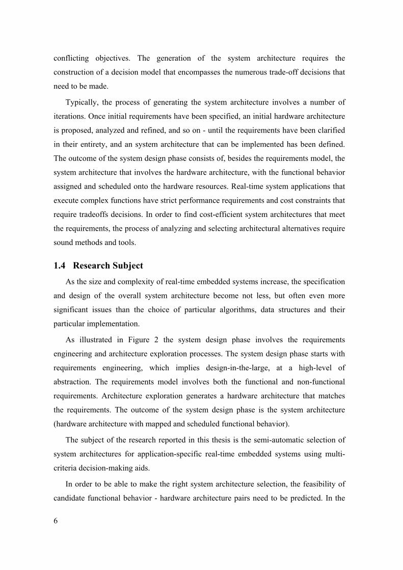
As illustrated in Figure 2 the system design phase involves the requirements
engineering and architecture exploration processes. The system design phase starts with
requirements engineering, which implies design-in-the-large, at a high-level of
abstraction. The requirements model involves both the functional and non-functional
requirements. Architecture exploration generates a hardware architecture that matches
the requirements. The outcome of the system design phase is the system architecture
(hardware architecture with mapped and scheduled functional behavior).
The subject of the research reported in this thesis is the semi-automatic selection of
system architectures for application-specific real-time embedded systems using multi-
criteria decision-making aids.
In order to be able to make the right system architecture selection, the feasibility of
candidate functional behavior - hardware architecture pairs need to be predicted. In the
7
architecture exploration phase, the generation of system architectures basically involves
three sub-problems that are strongly interrelated and need to be modeled and solved in a
joint manner:
Allocation determines the hardware architecture, that is, the types and number of
processing elements, and the network interconnecting these PE’s. The hardware modules
and the interconnection network in turn determine the processing element type.
RequirementsModel
Customer
SpecifyEngineering
History
SpecifyTests
UseCases
ArchitectureExploration
Allocate
Map &Schedule
ArchitectureAssessment
CODESIGN FLOW
SystemArchitecture
HardwareArchitecture
RequirementsEngineering
SYSTEM DESIGN PHASE
WorkloadEstimates
ArchitectureTemplate
Analyze
SystemArchitect
SystemArchitect
refine-ments
extract
SystemArchitect
Figure 2. System design flow
8
Mapping (or assignment) involves the assignment of all the behavioral sub-systems
(network of the system processes) on the hardware architecture (network of the
processing elements) in the light of the system parametric constraints and objectives.
Scheduling determines the order in which the processes and communication actions
mapped onto the processing elements are executed.
The method is semi-automatic, that is, the system architect first generates candidate
hardware architectures, analyzes the mapping and scheduling results, and generates
proposals for refinements. The mapping and scheduling is performed automatically by
heuristic search and involves the making of numerous trade-off decisions that meet the
system parametric constraints and objectives. During the heuristic search some
promising instantiations of the system architecture are proposed, estimated and selected
for further propagation.
The implementation of the heuristic search requires the construction of a decision
model, which consists of modeling elements for: the functional behavior, the hardware
architecture, mappings and schedules possible, and their costs and performance
relationships. The decision model furthermore includes a preference model for selecting
the most promising direction during the search. The more specific main subjects of the
research involve:
• the creation of a model, which is based on the requirements models, and which
characterizes the functional behavior, facilitates behavioral analysis, mapping and
scheduling, and properly expose the impact of system architecture decisions.
• the construction of the modeling constructs that defines the decision space for the
mapping and scheduling problem
• the construction of the heuristic search that is organized as a genetic algorithm for
predicting the feasibility of the candidate functional behavior – hardware
architecture pairs.
The problem specification and means for problem analysis and search of the design
space are also under design during the problem solving. The complexity, diversity, poor
structure and dynamic character of the system design problems require the system design
to be an evolutionary quality engineering process. The evolutionary design process is

9
then the most adequate solution for the system-level design problem solving [79] and is
adopted in this thesis.
1.5 Previous Works related to the Subject
Related previous work includes real-time system specification methods, studies for
architecture synthesis (hardware-software partitioning), distributed computing
(scheduling and allocation), problem solving organization and heuristic search.
The development of a real-time embedded system starts with its requirements
specification, which is an important and determining factor for the final outcome. For
example, UML [37] is a meta-modeling framework that can be tailored for a particular
application domain. For real-time systems, the Rapid Object-Oriented Process for
Embedded Systems (ROPES) methodology provides guidelines for the organization of
the design process. StateCharts models [59] [60] make part of UML; they are used to
model control-oriented sub-systems. System Description Languages (SDL) is used to
model telecommunications protocol software. The SDL-oriented Object Modeling
Technique (SOMT) provides guidelines for its use. Many more methods have been
developed [4] [76] [146] [147]. These methods are well established in industry; they are
however deployed mainly to capture the system functional requirements. Also software
can be generated using these models as starting point. They offer general modeling
support but are not well integrated with design that involves specialized hardware
architectures with multiple processors and accelerators.
Ptomely [17], Grape [99], OCAPI [141], System Studio [18], Colif [21],
SPI/FunState [41], MetroPolis [9], are examples of methods that start with models which
captures the system’s functional behavior and facilitates co-simulation also on
heterogeneous multi-processor architectures. In order to facilitate architecture
exploration at system-level, specialized models of computation are used that offer
application domain specific primitives. These methods typically advocate the separation
of component behavior and communication infrastructure and span multiple abstraction
levels. By stepwise refinement of the primitives and components, customization of the
model takes place and a model at a lower level of abstraction is obtained.
An important aspect of these specialized methods is the use of the internal design
representation for constructing methods and methods for system-level optimization

10
problems such as partitioning, allocation, scheduling and mapping problems. For
example, for architecture synthesis, scheduling and allocation problems typically start
with a task graph that represents the functional behavior. Such a task graph is however
only implicit present in the model and need to be extracted first [68] [150] [151].
The applications considered in this thesis have a mix of control and data-flow
functionality. In order to take the control behavior into account, specialized models need
to be constructed for the mapping and scheduling problem. Scheduling constraints that
hold for execution paths and for which CDFG’s are extracted are used in [54] [55] [56]
[136]. Tree-based scheduling has been proposed in [70]. In [96] a conditional
dependency graph is constructed from a high-level synthesis specification and
constraints-satisfaction programming is used for solving the optimization problem.
Conditional task graphs are used to model the scheduling problem at process level in [38]
[152]. The methods render static schedules, and execution time is the main concern.
Methods with which dynamic scheduling policies are obtained, instead of a static
schedule are studied in e.g. [30] [153]. These methods are based on research on the
scheduling and allocation of processes in distributed systems [3]. These methods are not
directly suited for systems that have a mix of control and data-flow functionality with
strong variability in the control flow, and many and strong data and control dependencies
between the processes.
The evolutionary design process is the most adequate solution for the system-level
design problem solving [79]. The evolutionary design process is brought into effect by
appropriately modeling the design problems, using the models and search tools equipped
in multi-objective decision-making aids to find, estimate and select some promising
alternative solutions, to analyze the solutions and model, and to accept them or start an
corrective action. A general discussion of genetic algorithms can be found in [5] [6] [7];
[32] discusses genetic algorithms with multiple objectives. Genetic algorithms have been
deployed for the hardware – software architecture synthesis problem [36] [155].
Although genetic algorithms are meta-heuristics, they require customization of the
design space representation and genetic operators [108]. Multi-criteria decision-making
(MCDM) methods facilitate the selection of intermediate solutions during the search. A
general discussion of MCDM can be found in [143] [124].

11
1.6 Problem Statement and Research Aims
The process of generating the hardware architecture (allocation) is a difficult design
task, and requires experienced system architects. Because design experience is difficult
to capture as an algorithm, the allocation process is very difficult to automate. System
architects benefit from the availability of methods and tools for what-if analyses. They
facilitate identification of the need to modify candidate hardware architectures and re-
iteration of the analysis.
The research aim is the development of a method for the semi-automatic selection of
system architectures for application-specific real-time embedded systems that make use
of heuristic search equipped with multi-criteria decision-making aids.
The decision model involves the problem of mapping and scheduling of hardware
architecture - functional behavior pairs; the allocation design task is not automated. The
decision model needs to be defined and consists of
1. Modeling elements representing the functional behavior
2. Modeling elements representing the hardware architecture
3. Modeling constructs which define the mappings and schedules allowed
4. Parametric constraints and objectives
5. Cost and performance estimates for the behavioral elements
6. Heuristic search algorithm (equipped with multi-criteria decision aids) with
which the decision problem is solved
The design process of an embedded system varies considerably with the application,
and there is a wide range of possible choices of models, abstractions, and representations.
However, common steps can be identified. Real-time embedded system applications are
naturally viewed to involve multiple processes that operate concurrently and
communicate with each other and the environment. In the research reported in this thesis,
SA/RT models [147] are used for modeling the system behavior.
The work on using SA/RT for co-design has been started and developed by VTT
Electronics [132] [133]. It consists of modeling and verification methods and tools. The
modeling method includes a system description language that is a combination of
Structured Analysis (SA) and VHDL. The structured analysis and structured design
(SA/SD) method [146] [154] is used in the requirements engineering phase to work out
12
and specify the real-time system requirements model. The SA/SD method is widely used
in industry [72] [117] [146], since the models used are simple enough to be intuitively
clear but capable of capturing the essentials of a system behavior. SA/RT (Structured
Analysis with Real-Time extensions) is no independent method but an upgrade of SA,
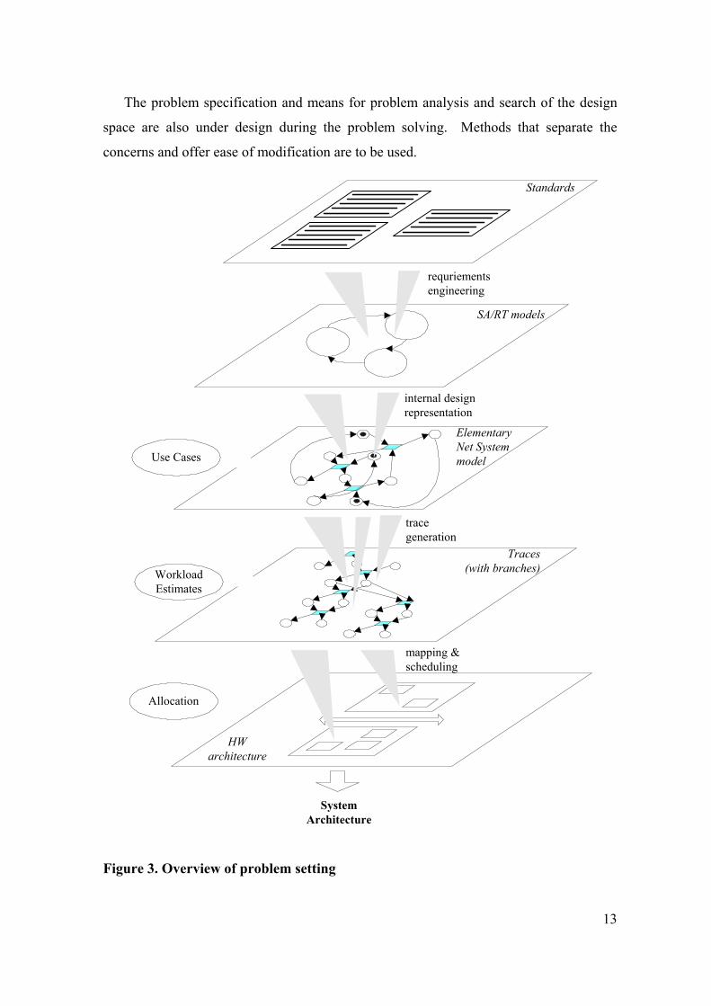
and is implied in this research. Figure 3 gives an overview of the problem setting.
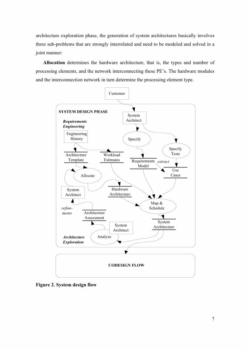
Typically, use cases can be identified that are representative for the system’s
functional behavior and for which certain costs and performance constraints apply.
Traces are then generated for these use cases and used as basis for performance and cost
analysis. Traces serve as input for the mapping and scheduling problem. The traces are
however not readily available. The execution rules of SA/RT models are semi-formal
and involve some ambiguities [11] [44]. Therefore, for behavioral analysis and in order
to be able to generate traces, execution rules need to be developed for SA/RT models that
take the original semi-formal execution rules as basis but exclude any of the ambiguities.
A SA/RT model includes both control and data-flow. Use cases typically involve
conditional actions; the corresponding traces split off. The part of the trace before the
branch represents the common behavior; the traces after the branch represent the
conditional behavior. For use cases that contain multiple conditional actions, the traces
split off in a tree-wise manner. The hardware architecture consists of a number of
processing elements containing hardware resources, and some interconnection network.
Allocation generates the hardware architecture. The process and communication actions
make up the traces, and require hardware resources. The assumption is made that
estimates of how long or the amount of resources needed for system and communication
actions can be given. The order in the processes and communication actions in the traces
take place specify the order in which hardware resources are requested. The mapping
configuration and scheduling decision determines which resources are assigned to which
behavioral elements, and in what order they use the resources respectively.
A decision model for the mapping and schedule problem needs to be constructed.
The interrelations between the behavioral elements (traces with branches), architectural
elements, mapping configurations and schedules, and associated costs and performance
define the decision space. The heuristic search method renders the strategy for finding a
satisfying solution within the decision space.
13
The problem specification and means for problem analysis and search of the design
space are also under design during the problem solving. Methods that separate the
concerns and offer ease of modification are to be used.
internal designrepresentation
tracegeneration
mapping &scheduling
Use Cases
WorkloadEstimates
requriementsengineering
Standards
SA/RT models
ElementaryNet Systemmodel
Traces(with branches)
SystemArchitecture
Allocation
HWarchitecture
Figure 3. Overview of problem setting
14
1.7 Main Assumptions and Solution Concepts
The paradigm and methodology of the quality-driven design proposed and discussed
by Jóźwiak in [79] [89] and his conference papers [80]-[88] [90] [91] give the main
theoretical and methodological base for the research reported in this thesis. The selection
method for system architectures for application-specific real-time embedded systems in
this thesis is a specific realization of the quality-driven design decision-making process
proposed by Jóźwiak [79] [87] [88] [91] and also discussed by Jóźwiak and myself in our
common early works on this subject [112] [113].
The methodology describes how the problem setting is to be organized when dealing
with ill-defined system design problems. Also it prescribes how combinatorial
optimization problem can be solved using heuristic search, equipped with multi-criteria
decision making aids for ranking the search operator alternatives, that is the search
direction.
The selection problem of system architectures makes part of the architecture
exploration phase. The allocation design task generates proposals for the hardware
architectures; potential performance bottlenecks and costs overruns, or resources’
underutilization, must be identified for the requirements model – hardware architecture
pair. A hardware architecture template, which defines a scalable and parameterized
hardware organization of the hardware resources, is used for generating the hardware
architectures.
The hardware architecture in this thesis consists of multiple processors and
accelerators, with an interconnection network for communication. For performance
reasons, the processors and accelerators have on-chip memories. The amount of
hardware resources used should be as little as possible, but sufficient to meet the non-
functional requirements. This especially applies for the on-chip memories, since they are
an important cost factor and a bottleneck in system performance.
The mapping configuration and scheduling decisions indirectly determine which and
when buffers and data objects of processes use on-chip memories. In this thesis, on-chip
memories are taken into account during mapping and scheduling in the architecture
exploration phase.

15
In order to predict whether the proposed hardware architecture is feasible for the
requirements model, the functional behavior is mapped and scheduled. Traces that
represent use cases that in turn represent the functional behavior, are the subject of this
mapping and scheduling. Use cases possibly contain conditional actions. The traces then
branches off in a tree-wise fashion.
The mapping and scheduling results give the system architect insight into which part
of the functional behavior is using what resources and when. The system architect uses
the mapping and scheduling results to identify potential bottlenecks and costs overruns,
or resources’ underutilization. In case they exist, the system architect proposes
modifications to the architecture, and the analysis is re-iterated.
The decision model for the selection problem includes a model of the decision space,
a preference model for alternatives in the decision space, the search method, and
preferences models for the search operators. The problem specification and means for
problem analysis and search of the design space are also under design during the problem
solving, since the models are not an objective reality and need to be constructed.
The decision space is for this reason first specified in terms of integer linear
programming (ILP) modeling constructs. The use of ILP modeling constructs offers ease
of modification and avoids any ambiguities in the specification. The search method is
however based on the meta-heuristics framework of genetic algorithms. The use of
heuristics methods instead of ILP optimization techniques is necessary since mapping
and scheduling optimization problems are well known to be NP-hard. The use of a meta-
heuristics framework over problem specific heuristics is preferred, since the problem
representation and search of the design space are separate matters; any modifications
remain local. The following concerns have been identified for constructing the decision
model.
Behavior Modeling and Generation of Traces – The SA/SD method and SA/RT
models are used to work out and represent the system’s functional behavior respectively.
The SA/SD method provides some guidelines for architecture exploration; they are
however merely hints. Moreover the execution rules for SA/RT are semi-formal –
deliberately.
SA/RT models are not directly suited for architecture exploration. In order to be able
to use SA/RT models as technical base for behavioral analysis and architecture

16
exploration, execution rules are needed that avoid any ambiguities in interpretation. An
important requirement for these execution rules is that they properly characterize the
application domain and hardware architectural primitives with which the models are
going to be implemented. Also, the modeling primitives used in the requirements model
need to have counterparts of which is known that they can be implemented effortless in
the system architecture model.
A key architectural decision is the selection of communication primitives and
connection topology used for inter-process communication. There needs to be tight
connections between the models at different level of abstractions. In the hardware
architecture assumed in this thesis, the main mechanism for inter-processing-elements
communication is by means of data movements between the on-chip memories. The
main mechanism for inter-processing-element communication involves the allocation of
on-chip memory space for buffering the data until it has been processed.
Communication primitives that are similar to those in CSP [64] [109] provide in the
requirements model a good abstract representation of the mechanisms used in the actual
hardware. In contrast to CSP however, the primitives adopted in this thesis exhibit true
concurrency [111] [120]. The distributed nature of system functionality implies that
communication and synchronization takes place asynchronously. This is an additional
reason for selecting CSP-like communication primitives.
The SA/RT method distinguishes a number of types of flows for communication and
synchronization. The flows are either asynchronous or synchronous. For architecture
exploration, only the data-flows that involve large amounts of data and synchronization
events that indicate the start/end of a process with considerable workload are relevant.
These communication and synchronization actions need to be exposed and represented
by CSP-like actions.
CSP-like primitives are well suited to model the communication actions taking place
between software and/or hardware processes. Also, they expose the data movements,
buffering needs, and implied state changes of the processes involved, which is of
importance for architecture exploration. The use of CSP-like primitives is in line with
communication using DMA or I/O with memory read/write bursts.
CSP-like communication primitives are also relatively simple to implement, so that
they don’t favor software or hardware; they can be used as an elementary modeling

17
primitive for both hardware and software. This is somewhat in contrast to FIFO queues,
which can be implemented easily in software, but requires some deliberation when used
in hardware since it introduces a separate hardware module and possibly some latency
that is can only be exposed with simulation during requirements engineering.
It is also of importance to be able to make expose the concurrent behavior and the
causal relations that exist between the elementary processes and communication actions
that account for most of the resources use. The use of CSP-like primitives makes it
possible to obtain traces that represent the partial order and conflict relations between
these process execution runs and the occurrences of communication actions. Traces can
be obtained by unfolding of the SA/RT model on the basis of representative use cases.
Events are conflicting if they occur in different branches of the trace.
Unfortunately, there is no one-to-one translation possible of the control and data-
flows found in a SA/RT model, into CSP-like primitives such that they comply with the
original semi-formal execution rules. A set of execution rules that are based on the semi-
formal ones, but does not exhibit the ambiguities need to be developed. The work
includes the development of a method to translate the control and data-flows of a SA/RT
model into CSP-like primitives.
Elementary net systems [126] [149] are used as internal representation model.
Elementary net systems provide a framework for behavioral analysis in this thesis and
are a fundamental sub-class of Petri Nets [120]. The elementary net system
representation of a concurrent (simultaneous) system consists of local states, local
transitions (between the local states) and the flow relationship between the local
transitions and the local states. The unfolding of elementary net system results in traces
with possible branches. For elementary systems, traces involve event structures [149].
The elementary net systems representation of a sequential process can be obtained in
a straightforward manner. In this thesis a construction method for elementary net systems
that represent concurrent (simultaneous) systems that consist of a number of sequential
processes is proposed. The construction method renders the joint behavior as an
elementary net system that contains the same local states as the original component
processes (or transformations). The joint behavior is obtained by “multiplying” the
component elementary net system representations of the elementary processes. The
elementary net systems obtained behave similar to the original SA/RT models;

18
ambiguities do not exist since they are resolved by the execution rules in some specific
way.
Hardware Architecture Model – In order to be able to predict the feasibility of
hardware architecture – requirements model pairs, modeling constructs need to be
formulated for the decision model for the mapping and scheduling problem. The
hardware architecture model distinguishes resources that are at the disposal of the
processes and communication actions. The resources are associated with the hardware
modules included in the hardware architecture. The resources need to be shared or have
some limited capacity. Resources that are relevant for the assessment need to be exposed
in the decision model.
The real-time embedded systems considered belong to a relatively limited, well-
defined, well-known, analyzed and characterized system class, so that a certain general
solution form (generic architecture template) is known (or can be effectively developed)
for the systems of this class, and a particular system architecture for a particular system
of this class can be obtained by a certain instantiation of this general form. However, the
class of the considered systems is not so much limited and not so well known, analyzed
and characterized that a parameterized architecture generator can be built for the whole
class, and a particular system architecture can be obtained by setting the generator
parameters to certain values and by simple generation. The particular architecture and
mapping and scheduling must be constructed for a particular system, in the light of the
system parametric constraints, objectives and trade-off information.
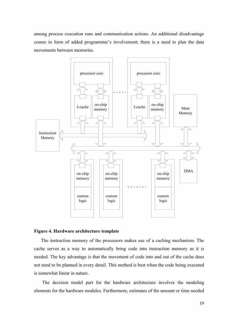
The hardware architecture template is illustrated in Figure 4. For architecture
exploration four kind of modules are distinguished: processing element units (processor
and custom logic), on-chip memory, DMA channels, and memory ports. These hardware
modules are shared resources that can be requested for by the processes and
communication actions in the order in which they occur in the traces.
The hardware architecture template adopted in this thesis, assumes on-chip memory
that serves as scratchpads for data. The advantage of using scratchpads over caches is
that memory access is relatively fast and access time can be guaranteed. For large
amounts of data and time-critical operation, the use of scratchpads offers full control of
the hardware, as compared to the use of caches. The trade-off is their high price. Because
of cost-efficiency, on-chip memories’ capacity is limited and they need to be shared
19
among process execution runs and communication actions. An additional disadvantage
comes in form of added programmer’s involvement; there is a need to plan the data
movements between memories.
processor core
I-cache on-chipmemory
on-chipmemory
customlogic
on-chipmemory
customlogic
on-chipmemory
customlogic
processor core
I-cache on-chipmemory
DMA
MainMemory
InstructionMemory
Figure 4. Hardware architecture template
The instruction memory of the processors makes use of a caching mechanism. The
cache serves as a way to automatically bring code into instruction memory as it is
needed. The key advantage is that the movement of code into and out of the cache does
not need to be planned in every detail. This method is best when the code being executed
is somewhat linear in nature.
The decision model part for the hardware architecture involves the modeling
elements for the hardware modules. Furthermore, estimates of the amount or time needed
20
by behavioral elements for the various modules make part of the decision model. The
SA/RT follows a top down approach. The design process is however in practice a mix of
top down and bottom up design. Estimates of the costs for or the time needed by some
behavioral element to use a certain hardware module can be given. The estimates can, for
example, be based on the incomplete functional specification of the elementary
processes, or on the engineering history.
System Architecture Model – The modeling constructs for the functional behavior
and hardware architecture provides a simplified and approximate view of how the
functional behavior progresses and how the hardware operates. The outcomes of which
and when resources are used are only approximations. The creation of the system
architecture however still requires consideration of a great deal of information. Each
process executes at different speeds on different PE’s. PE’s possibly vary in the
functional units included, communication topology, on-chip memories and memory
bandwidth.
Architecture design needs to take the utilization of PE’s, inter-process
communication, component cost, and other factors into account. The modeling constructs
for the functional behavior and the hardware architecture form the base modeling
constructs of the decision model. The modeling constructs formulated for the system
architecture, tie them together. The system architecture part of the decision model
defines the interrelationships that cover more than individual processes, communication
actions, or hardware modules. The system architecture modeling constructs describes
approximately the mechanisms for resource sharing.
The formulation of constructs that model the on-chip memory use by communication
actions is an issue that cannot be considered in isolation. The communication actions in
real-time embedded systems that involve large amounts of data-flows with distributed
multi-processor hardware architecture require considerable use of resources and are
subject for optimization.
Dependent on the availability of DMA in the hardware architecture, the
communication actions make use of DMA or I/O based inter-PE communication. Also,
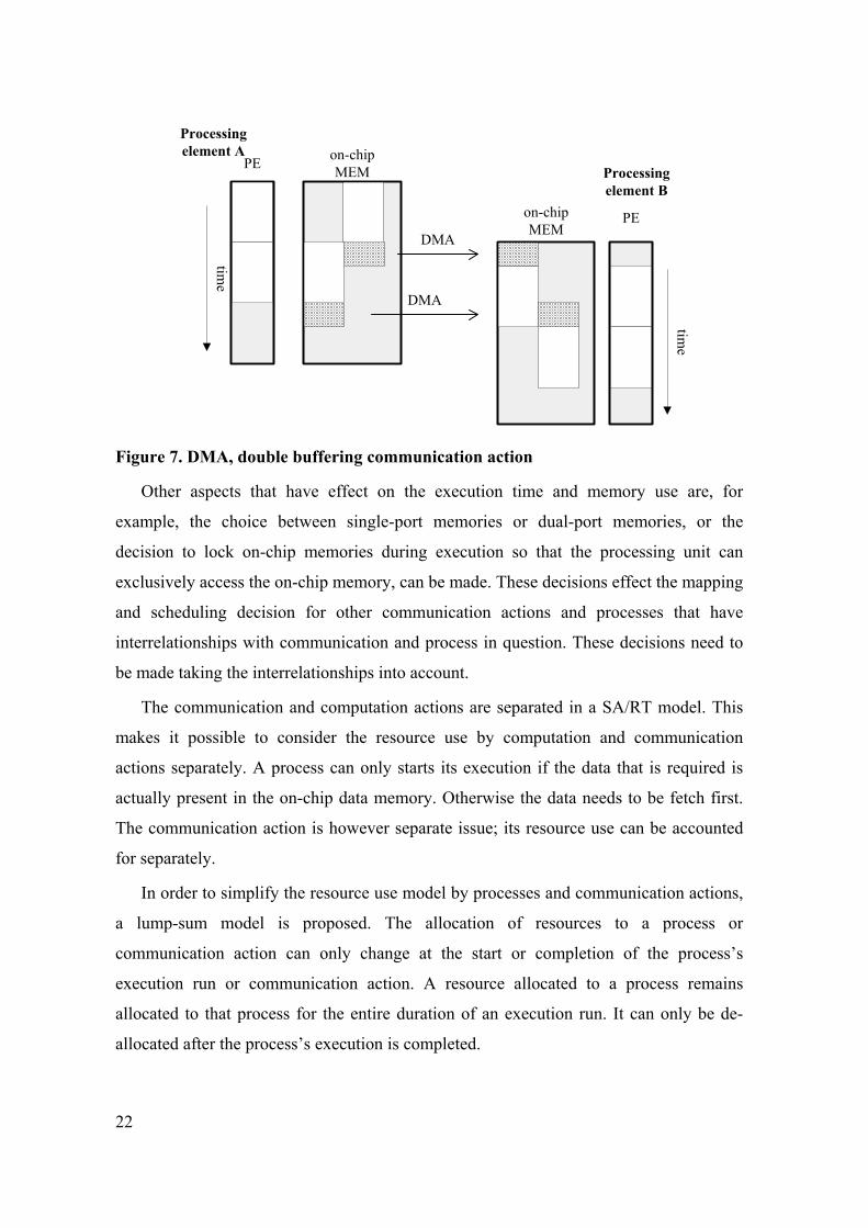
communication actions use double or single buffering. Communication actions are typed.
Single buffering means that a new communication action can only start if a previous
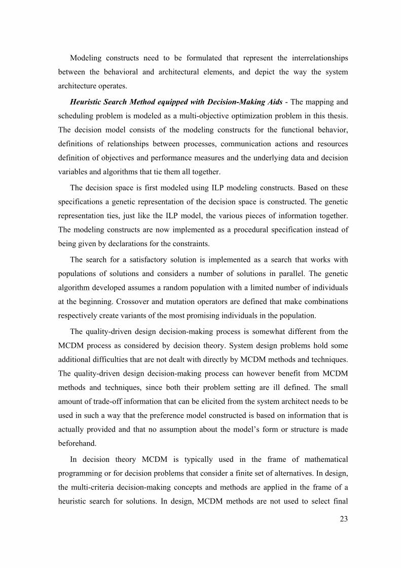
communication of the same type has been completely processed. Double buffering
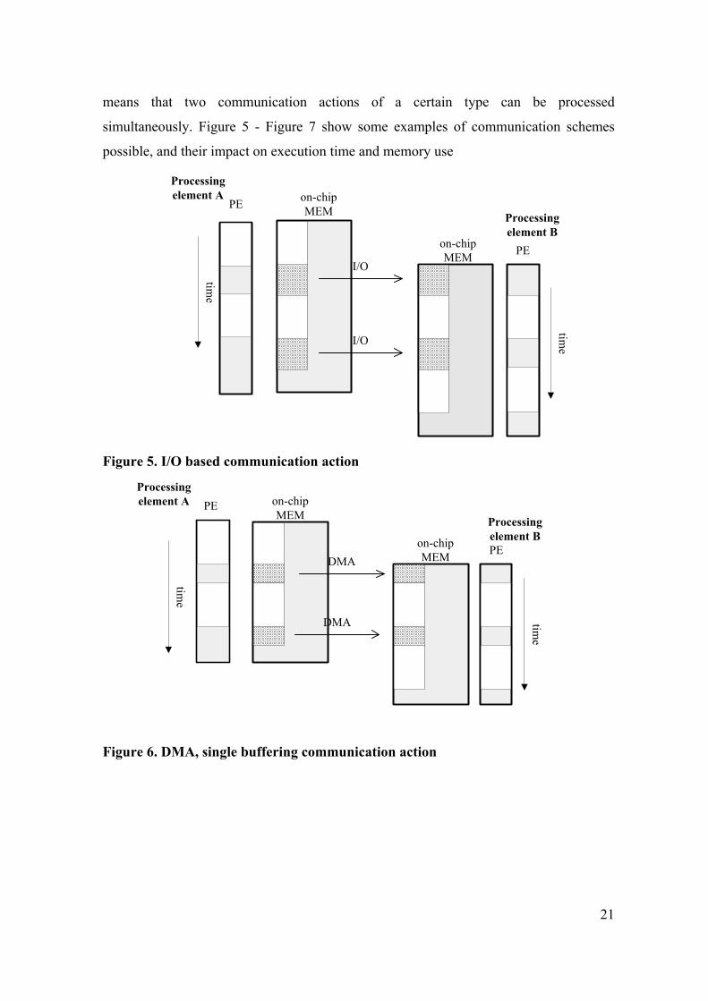
21
means that two communication actions of a certain type can be processed
simultaneously. Figure 5 - Figure 7 show some examples of communication schemes
possible, and their impact on execution time and memory use
Processingelement A
Processingelement B
PE
time
on-chipMEM
PE
time
on-chipMEM
I/O
I/O
Figure 5. I/O based communication action
Processingelement B
Processingelement A
time
PE on-chipMEM
time
PEon-chipMEMDMA
DMA
Figure 6. DMA, single buffering communication action
22
Processingelement B
Processingelement A
PE on-chipMEM
time
PEon-chipMEM
time
DMA
DMA
Figure 7. DMA, double buffering communication action
Other aspects that have effect on the execution time and memory use are, for
example, the choice between single-port memories or dual-port memories, or the
decision to lock on-chip memories during execution so that the processing unit can
exclusively access the on-chip memory, can be made. These decisions effect the mapping
and scheduling decision for other communication actions and processes that have
interrelationships with communication and process in question. These decisions need to
be made taking the interrelationships into account.
The communication and computation actions are separated in a SA/RT model. This
makes it possible to consider the resource use by computation and communication
actions separately. A process can only starts its execution if the data that is required is
actually present in the on-chip data memory. Otherwise the data needs to be fetch first.
The communication action is however separate issue; its resource use can be accounted
for separately.
In order to simplify the resource use model by processes and communication actions,
a lump-sum model is proposed. The allocation of resources to a process or
communication action can only change at the start or completion of the process’s
execution run or communication action. A resource allocated to a process remains
allocated to that process for the entire duration of an execution run. It can only be de-
allocated after the process’s execution is completed.
23
Modeling constructs need to be formulated that represent the interrelationships
between the behavioral and architectural elements, and depict the way the system
architecture operates.
Heuristic Search Method equipped with Decision-Making Aids - The mapping and
scheduling problem is modeled as a multi-objective optimization problem in this thesis.
The decision model consists of the modeling constructs for the functional behavior,
definitions of relationships between processes, communication actions and resources
definition of objectives and performance measures and the underlying data and decision
variables and algorithms that tie them all together.
The decision space is first modeled using ILP modeling constructs. Based on these
specifications a genetic representation of the decision space is constructed. The genetic
representation ties, just like the ILP model, the various pieces of information together.
The modeling constructs are now implemented as a procedural specification instead of
being given by declarations for the constraints.
The search for a satisfactory solution is implemented as a search that works with
populations of solutions and considers a number of solutions in parallel. The genetic
algorithm developed assumes a random population with a limited number of individuals
at the beginning. Crossover and mutation operators are defined that make combinations
respectively create variants of the most promising individuals in the population.
The quality-driven design decision-making process is somewhat different from the
MCDM process as considered by decision theory. System design problems hold some
additional difficulties that are not dealt with directly by MCDM methods and techniques.
The quality-driven design decision-making process can however benefit from MCDM
methods and techniques, since both their problem setting are ill defined. The small
amount of trade-off information that can be elicited from the system architect needs to be
used in such a way that the preference model constructed is based on information that is
actually provided and that no assumption about the model’s form or structure is made
beforehand.
In decision theory MCDM is typically used in the frame of mathematical
programming or for decision problems that consider a finite set of alternatives. In design,
the multi-criteria decision-making concepts and methods are applied in the frame of a
heuristic search for solutions. In design, MCDM methods are not used to select final

24
alternatives; they are used to select intermediate solutions in the heuristic search and to
specify the system architect’s preferences in a convenient, actual and robust manner. The
problems of constructing a preference model are the same in decision theory and design.
Preferences are specified interactively using aspiration points [101] in this thesis. During
parallel search, a limited number of the most promising alternatives are selected for
crossover and mutation; this selection is based on the preference model constructed.
Utility functions are typically used in decision theory to aggregate the individual
criteria into a single criterion. The ill definiteness of the problem setting makes them
unsuitable. Outranking methods require less trade-off information and less modeling
parameters from the system architect [23] [143]. These methods are less extensive than
methods based on utilities. Outranking methods however still require too much
information from the system architect for the mapping and scheduling problem in this
thesis. An enhanced version of the non-dominated sorting method [23] has been
developed and is used to rank the intermediate solutions in the heuristic search.
The parallel search starts with initializing the population by constructing random
solutions. The most promising candidates are selected for combination and mutation. The
population size is limited; only the most promising candidates among the newly created
individuals and those already present in the population can be selected into the next
generation population. Distance measures in the objectives space are constructed to
define the closeness of individuals. These measures are used as secondary criteria for
selecting the individuals in order to guarantee diversity of the populations.
Constraints cannot be handled in a straightforward manner by genetic algorithm since
the operators for mutation and re-combinations are blind to constraints [28]. It is not
guaranteed that the offspring of parents that meet the constraints satisfy them as well.
Constraints handling is managed by replacing constraints by optimization objectives that
minimize the constraints’ violations.
The search method in this thesis makes use of sensitivity information. Objectives
possibly have varying sensitiveness towards changes in values of the decision variables
in the model. In order to reduce the decision space, the values for the decision variables
that have the smallest impact do not need to be determined at first. In order to still
incorporate their impact,, they are set to values that cause the objectives to take on a
combination of minimum and maximum values. The objective values for a solution has

25
undefined decision variables. Values are not crisp, but are given by interval ranges. The
sorting or ranking problem becomes a problem with fuzzy numbers [23].
The genetic algorithm obtains solutions that involve a set of decision variables of
which a sub-set are unknown. In case these decision variables make part of constraints
that are difficult to handle with GA, CSP can be used to determine their values. Genetic
algorithm is then deployed to first determine the overall search direction; CSP is used to
resolve the values of the remaining decision variables.
1.8 Main Contribution and Outline of Work
The main contribution is the development of a method to predict the feasibility of
specific hardware architecture – requirements model pairs. This contribution includes the
contributions in the following areas.
Organization of Problem Solving Process - In this thesis, a specific and original
realization of the quality-driven design paradigm as proposed by Jóźwiak [79] has been
developed for solving the mapping and scheduling problem of requirements model –
hardware architecture pairs for architecture exploration in the system-level design phase.
It is argued that the system design problems need to be modeled first due to their
complexity, diversity, poor structure and dynamic character; the model is only a
subjective representation of reality that evolves along the course of its development. The
evolutionary design process is implemented by appropriately modeling the design
problems, using the models and search tools equipped with multi-criteria decision-
making aids to find, estimate and select some promising alternative solutions.
Exposure of the On-chip Memory Use and Communication - Distinct from other
system architecture synthesis approaches, the mapping and scheduling of memory use by
processes and communication actions is integrated in the mapping and schedule problem.
Memory aspects such as memory locking can also be included in the decision model.
Communication actions are usually modeled to only consume time, and bus capacity.
Memories and memory ports are hardware primitives, and just like other primitives they
can be assigned and scheduled for some time to process, communication actions, or data
objects. The mapping configuration and precedence and conflict relations between the
elements determine which memory is to be assigned to what functional element and for

26
how long. Novel and original modeling constructs have been developed that approximate
the use patterns of these memories.
Execution Rules, Translation Method, Traces Extraction for SA/RT Models – The
execution rules of SA/RT is semi-formal. New and original execution rules have been
developed which formalizes the behavior of SA/RT. Also, a novel construction method
has been developed with which a SA/RT model can be translated into and represented as
a set of communication processes that use CSP-like communication and synchronization
actions; the construction method translates SA/RT models into elementary net systems.
Difficulty hereby is that SA/RT models are in origin a mixed synchronous/asynchronous
models; primitive flows in the SA/RT need to be grouped and cast onto their
asynchronous counterpart. Execution rules are a pre-requisite to extract traces (with
branches) from the SA/RT model based on some use case. These traces form a
representation of the functional behavior of the SA/RT model and serves as input for the
mapping and schedule decision model. Various abstract behavior models that enable
static timing and resource analysis based on traces for SA/RT models, together with
timing and resource usage estimation procedures have been developed in this thesis. The
estimation procedures make use of an abstraction of the hardware resource
characteristics.
Heuristics Search Method for Mapping and Scheduling – A new deployment
scheme for GA and CSP for optimization has been developed. The scheme makes use of
sensitivity information; the decision variables for which the solution has a high
sensitivity are resolved first. In a second (post-processing) stage the remaining decision
variables that are possibly difficult to solve using GA due to the constraints involved, are
set. Also, the non-dominated sorting method has been enhanced, in order to better
discern the alternatives mutual ranking.
All parts have been extensively analyzed and tested, and have been checked together
on some examples.
Outline of Work:
Chapter 2 gives an introduction to real-time embedded systems and their modeling. It
discusses the SA/SD system specification method and the SA/RT models, and motivates
the choice to implement the communication action in SA/RT models using rendezvous.

27
Chapter 3 discusses decision making for system design. The mapping and scheduling
in system problem setting is not an objective reality and needs to be modeled. In this
aspect the problem resembles that of multi-criteria decision making (MCDM) as
discussed by decision theory. The chapter gives an overview of MCDM and points where
system design decision-making can benefit from MCDM. Genetic algorithms are passed
in review, since the search and optimization process for the mapping and scheduling
problem is using these meta-heuristics.
Chapter 4 discusses the approximate behavior attached to the SA/RT models. A
SA/RT model is first represented in terms of state machines, which involves the
significant system states and transitions. The state machines are reasonably represented
by transition systems, since they embody a distributed system and distributed
computations. Because the SA/RT execution rules make a distinction between
synchronous and asynchronous communication, the transition system contain two types
of transitions. In order to only have asynchronous communication, elementary transitions
or grouped into multi-event transitions, or multi-events. The grouping and the behavior
of multi-event transitions are discussed.
Transitions systems are well suited for behavioral analysis; they are however an
interleaving concurrency model and only make a relatively less manageable
implementation of a composition operator possible. For this reason elementary net
systems (sub-class of Petri Nets) are used as an internal model. They are discussed in
Chapter 5. The discussion includes that of the composition operator for combining
component elementary net systems and auxiliary notions for the construction method.
Chapter 5 also discusses the construction method for the multi-event transitions.
Chapter 6 discusses the optimization model for mapping and scheduling the
behavioral model onto the target architecture. The decision space of the mapping and
scheduling problem is first given as a linear system, which serves as specification for the
genetic representation with specialized data structures. Modeling constructs that
embodies the most important issues are given
In Chapter 7 the concepts and methods introduced are deployed for design cases.

28
29
Chapter 2.
Modeling of Embedded Systems
2.1 Introduction
The research reported in this thesis uses the Structured Analysis and Structured
Design (SA/SD) method [146] and Structured Analysis and Real-Time extensions
models (SA/RT) models [147] for the requirements engineering phase of system design.
The SA/SD method provides full life-cycle support from the initial product specification
through to implementation. A SA/RT model is a homogeneous modeling notation; the
SA/SD method is an integrated approach for the engineering of real-time systems.
SA/RT models can already be deployed at the early design stages, that is, already in the
system analysis phase, before implementation details are added.
The SA/SD method follows a top-down approach, and renders the structure for the
behavioral model of the system. The model consists of a set of processes (or
transformations) and their interconnections (or flows) and involves a process hierarchy.
The SA/RT models are basically event-based and represent a set of concurrent processes
that communicate and synchronize with each other using some form of message passing.
The primitive processes at the leaves and the connectors are the elementary building
blocks of an SA/RT model. SA/RT models are typically used for system applications that
involve a mix of control and data processing functionality.
Because of the complex communication and synchronization patterns present in
concurrent systems, it is difficult for system architects to understand and reason about
these systems. Thus, it is important that behavioral analysis techniques are developed
that assist in understanding of these systems. For the mapping and scheduling problem in
the system design phase, there is most often no point in analyzing the precise places and
30
times of operations or instructions in a distributed computation. What is generally
important, is to monitor the significant events and how the occurrence of an event
causally depends on the previous occurrence of others. For example, the event of a
process transmitting a message would presumably depend on it first performing some
events, so it was in the right state to transmit, including the receipt of the message, which
in turn would depend on its previous transmission by another process. These causal
dependencies form the precedence constraints between the processes and are of
importance for working out the mapping and scheduling problem.
The causal dependencies for the processes involved in use cases that represent typical
system behavior or expose the system’s bottlenecks are computed. The requirements
model usually includes the specification of system functionality, or use cases for which
some non-functional constraints apply. In this thesis, use cases are modeled in terms of
sequences of system input actions; the sequences serve as stimuli for the behavioral
system model. System execution runs are obtained as outcome for these input sequences.
The requirement for certain system functionality to comply with some non-functional
constraints means that their use cases’ system execution runs need to meet these
constraints.
In the research reported in this thesis an approximate behavior is attached to the
SA/RT model for behavioral analysis, by specifying state machines for the primitive
processes. The state machines represent the important states in the processes, and the
operations that cause the transitions between these states. Besides the state machines, the
connectors (branches, merges, flows) and the mechanisms involved for the
communication and synchronization between the processes define the overall system
behavior in a significant way. A selection of mechanisms is possible and its choice
depends on the system application and hardware architecture at hand. Examples for the
communication mechanisms are message-passing protocols such as FIFO, shared
memory, and data streams. The research reported in this thesis aims to use
communication primitives that match the system applications and hardware architecture
described in Chapter 1.
The behavior is formally modeled in terms of labeled transition systems (LTS). In
particular, behavior is attached to the SA/RT model by specifying a labeled transition
system for each primitive component in the SA/RT model. LTS makes use of
31
rendezvous; the communication mechanism used is CSP-like. An LTS contains all the
reachable states and executable transitions of a process. The behavior of the composite
LTS is computed from its constituent parts. For this computation, all necessary
information related to the structure and interconnections of components is extracted from
the state machines and structural description of the system. The hardware architecture
involves multiple processors and accelerators, and embodies a fully distributed system
architecture. LTS models have been widely used in the literature for specifying and
analyzing distributed systems; also in this thesis, labeled transition systems (LTS) are
used to model the behavior of the communicating processes.
The system architecture’s distributed character justifies the choice of the rendezvous
primitive. This primitive is considered sufficient to capture the interactions in a SA/RT
models. Although the two-way rendezvous is an atomic action, it implies the occurrence
of a pair of actions in reality, distributed over two interacting processes, a sender and a
receiver. In this thesis, rendezvous actions that jointly take place and have a fixed pattern
are furthermore grouped together and rendered as atomic actions in the LTS model in
order to simplify the behavioral analysis.
The use cases for certain system execution runs and the constraints associated with
them, are input to the mapping and scheduling problem. For scheduling, the pattern of
events that represent the system execution run needs to exhibit how the occurrence of
certain system actions causally depends on the occurrence of others. Execution run are
therefore rendered as occurrences of system actions together with a relation expressing
their causal dependencies; this is reasonably a partial order. Also, it is considered
desirable to express how certain occurrences of system actions rules out the occurrence
of others; the conflict relation specify whether pairs of events exclude one another.
Event structures are exactly representing these relationships and for this reason suited
to represent system execution runs; an event structure , ,E confl≺ renders the causal
dependency relation ≺ and conflict relation confl for a set of events E . Unfortunately,
the event structures for the system execution runs cannot be obtained directly from the
LTS system, since LTS is an interleaving behavioral model. One main distinction in the
classification of behavioral models for concurrent systems is that between interleaving
and non-interleaving models. The main characteristics for an interleaving model is that it
abstracts away the true concurrency of system events; the system behavior is expressed
32
in terms of non-deterministic merging, or interleaving of occurrences of system actions.
The unfolding of a LTS behavioral model for a sequence of input system actions results
in a sequence of interleaved system events, which does not display the partial ordering.
Event structures can be constructed in a straightforward manner by the unfolding of
elementary net systems [126] [149]. Elementary net systems are a sub-class of Petri Nets
and are a non-interleaving behavioral model for concurrent systems. An elementary net
system representation of the LTS system behavioral model is for this reason constructed
in this thesis. The system behavior is however not directly specified as an elementary net
system, since abstract mechanism for process interactions are not integrated in
elementary net systems. LTS’s on the other hand offer well-defined execution rules for
the communication and synchronization of system actions distributed over multiple
processes.
In this thesis, component elementary net systems for the individual component LTS’s
are first constructed. They are combined using a multiplication operator in order to
obtain the composite elementary net system from the component LTS’s. The elementary
net system representation is not constructed directly from the composite LTS of the
primitive processes and connectors, since this is computationally very costly and for this
reason not practical. The composite elementary net system represents the composite
LTS, and exhibits the joint LTS-compliant behavior of the primitive processes and
connectors cooperating.
2.2 SASD Method
The Structured Analysis with Real-Time Extension (SA/RT) model is briefly
overviewed in this section. SA/RT models are deployed in combination with the
Structured Analysis and Structured Design (SASD) method [146], and are predominantly
applied in technical, real-time-oriented applications. In particular, the SASD method is in
line with, and can be used to implement the design process and the system design phase
for real-time embedded systems as described in Chapter 1; the first two phases
distinguished in the SASD method, addresses the same concerns as the system design
phase. Also, the SASD method versatility makes it suitable to support an evolutionary
design process.

33
A system development cycle is described as a step-by-step breakdown of the system
development process for understanding, organizing and planning the system
development and maintenance process. Many enhancements and extensions have been
introduced since the introduction of the SASD method two decades ago. The SASD
method currently provides a powerful set of concepts and methods, which addresses the
typical main stages of a system development cycle, and real-time systems in particular.
The SASD method distinguishes the analysis phase, the design phase, the
implementation phase, the utilization phase, and the maintenance phase. The system
design phase as introduced in Chapter 1 is addressed by the analysis and design phases in
the SASD method.
The goal of the analysis phase is to create a description of what is desired and what
eventually need to be developed. The desired output of this phase is, in short, a statement
of what the system must do and which features it should expose. The analysis phase only
aims at the specification of the requirements, and does not consider the implementation
details of processes, tasks or functions. The analysis phase provides input to the design
phase.
The goal of the design phase is to provide a model of the solution, which involves a
logical model and a physical model. The logical model represents the system behavior,
but does not consider system resources, resource constraints, programming language
features, or other implementation concerns; first the physical model takes them into. The
physical model represents the functional behavior mapped onto a network of coarse grain
structural components such as processors and (re-configurable) hardware co-
processors/accelerators; physical models correspond to system architectures as
introduced in Chapter 1. The design phase does however not include any implementation
details; only abstract physical models are constructed to model some implementation
aspects that are sufficiently precise to enable effective and efficient system analysis and
decision-making.
The goal of the implementation phase is to actually construct the system solution
according to the physical model from the design phase. In the implementation phase, the
actual hardware and software are being constructed based on the pseudo-code and the
actual target architecture developed.

34
System development cycle models differ in the way development time and
importance are assigned to the different phases, and how the phases relate with each
other. SASD has been used in conjunction with a number of software lifecycles models.
The interdependencies between the system design tasks impose a certain ordering of
phases in the development process.
For routine standard design settings, SASD can be used to support the waterfall
system development cycle model. The waterfall model is a well-known model that
adopts a phased approach. Although there are interactions between the phases, there is a
clear separation and linear ordering of the development stages. In routine design the
interdependencies between the models and phases are known beforehand. The various
phases included by the SASD method is then progressed in a linearly ordered phased
manner.
For relatively new and complex systems the development issues, task and model
interrelationships are not known beforehand. The development process does not involve
easily distinguishable and linearly ordered steps with identifiable start and ending points.
The entire process of analysis, design and implementation is considered to be the
evolutionary development and continuous refinement of a series of models. The impact
(tentative) design decisions have, can only be anticipated at the moment the decisions are
actually being made. This is a different angle than traditional routine design takes. For
relatively new and complex systems, the more general continuous evolutionary design
process is therefore much more suited than the linearly ordered process (that is in fact a
very special case of the evolutionary design process). Due to its versatility, SASD can
also be used to support the evolutionary design process.
2.3 SA/RT Models
The SASD method using SA/RT models (or SA/RT method in short) includes a
number of models and views, which combined render the system view. The components
of the SA method are
• data-flow diagrams (DFD),
• process hierarchy,
• means to represent the process specification (e.g. pseudo code, structured text,
diagrams, formulas, labeled graphics),
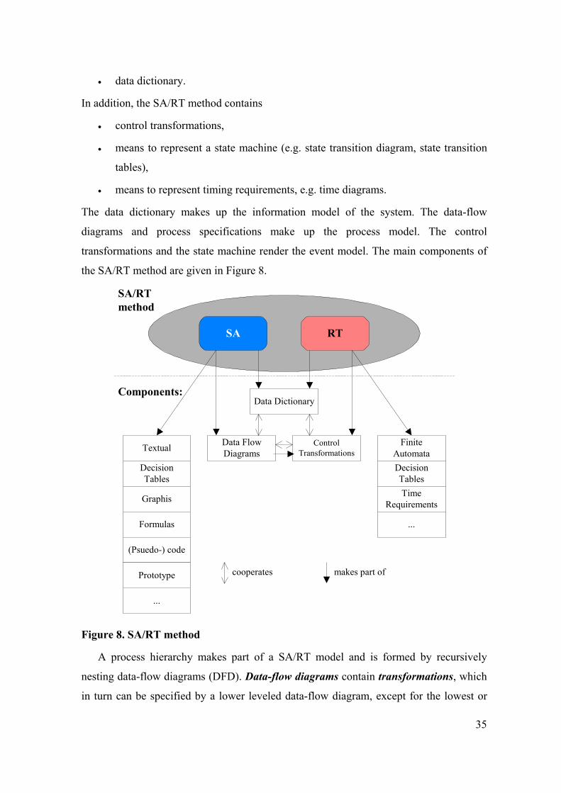
35
• data dictionary.
In addition, the SA/RT method contains
• control transformations,
• means to represent a state machine (e.g. state transition diagram, state transition
tables),
• means to represent timing requirements, e.g. time diagrams.
The data dictionary makes up the information model of the system. The data-flow
diagrams and process specifications make up the process model. The control
transformations and the state machine render the event model. The main components of
the SA/RT method are given in Figure 8.
Data FlowDiagrams
ControlTransformations
Data Dictionary
FiniteAutomataDecisionTablesTime
Requirements
...
Textual
DecisionTables
Graphis
Formulas
(Psuedo-) code
...
SA RT
makes part ofcooperates
Components:
SA/RTmethod
Prototype
Figure 8. SA/RT method
A process hierarchy makes part of a SA/RT model and is formed by recursively
nesting data-flow diagrams (DFD). Data-flow diagrams contain transformations, which
in turn can be specified by a lower leveled data-flow diagram, except for the lowest or
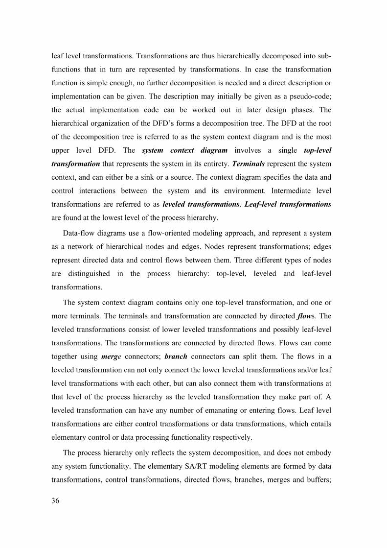
36
leaf level transformations. Transformations are thus hierarchically decomposed into sub-
functions that in turn are represented by transformations. In case the transformation
function is simple enough, no further decomposition is needed and a direct description or
implementation can be given. The description may initially be given as a pseudo-code;
the actual implementation code can be worked out in later design phases. The
hierarchical organization of the DFD’s forms a decomposition tree. The DFD at the root
of the decomposition tree is referred to as the system context diagram and is the most
upper level DFD. The system context diagram involves a single top-level
transformation that represents the system in its entirety. Terminals represent the system
context, and can either be a sink or a source. The context diagram specifies the data and
control interactions between the system and its environment. Intermediate level
transformations are referred to as leveled transformations. Leaf-level transformations
are found at the lowest level of the process hierarchy.
Data-flow diagrams use a flow-oriented modeling approach, and represent a system
as a network of hierarchical nodes and edges. Nodes represent transformations; edges
represent directed data and control flows between them. Three different types of nodes
are distinguished in the process hierarchy: top-level, leveled and leaf-level
transformations.
The system context diagram contains only one top-level transformation, and one or
more terminals. The terminals and transformation are connected by directed flows. The
leveled transformations consist of lower leveled transformations and possibly leaf-level
transformations. The transformations are connected by directed flows. Flows can come
together using merge connectors; branch connectors can split them. The flows in a
leveled transformation can not only connect the lower leveled transformations and/or leaf
level transformations with each other, but can also connect them with transformations at
that level of the process hierarchy as the leveled transformation they make part of. A
leveled transformation can have any number of emanating or entering flows. Leaf level
transformations are either control transformations or data transformations, which entails
elementary control or data processing functionality respectively.
The process hierarchy only reflects the system decomposition, and does not embody
any system functionality. The elementary SA/RT modeling elements are formed by data
transformations, control transformations, directed flows, branches, merges and buffers;

37
after collapsing the process hierarchy these building blocks remain and form the
primitive processes and connectors. The execution rules for the primitive processes and
connectors are the following.
Figure 9 shows an example process hierarchy that involves three levels. The system
context diagram is given by DFD1, and consists of the top-level transformation and the
terminals t1, t2, and t3. The top-level transformation consists is worked out in DFD2 and
consists of a control transformation and the leveled transformations Prod and Proc. Upon
s1 or s2 becoming active, Prod generates output o. Proc processes o and generates q as
result. Transformations Proc and Prod are further decomposed. They are specified by
DFD3 and DFD4 respectively. The transformations ctrl, prod1, prod2, prodA and prodB
are leaf-level transformations. The state machines in Figure 9 describe the behavior of
these transformations. Figure 9 contains the most important modeling element of an
SA/RT model. The modeling elements of an SA/RT model are described as follows.
Data transformations (DTR) entail a sequential procedure or program region that is
invoked upon receiving an active input. After a non-deterministic but greater than zero
time delay, the data transformation completes its execution and generates one or more
outputs. The data transformation embodies those parts of the system that involve low-
level functions that transform data input into data output(s), create stored data based on
data input, transform previously stored data into data output(s), report the occurrence of
events by generating control signals. Solid circles graphically depict data
transformations.
Control transformations (CTR) model the control behavior of the system and keep
track of the overall system state. They regulate the behavior of the data transformations
based on the overall system state. Control transformations are state machines; upon
receiving an input, the transition is carried out and output generated. The input, transition
and generation of output takes place in virtual zero time. Control transformations are
graphically depicted as dotted circles.
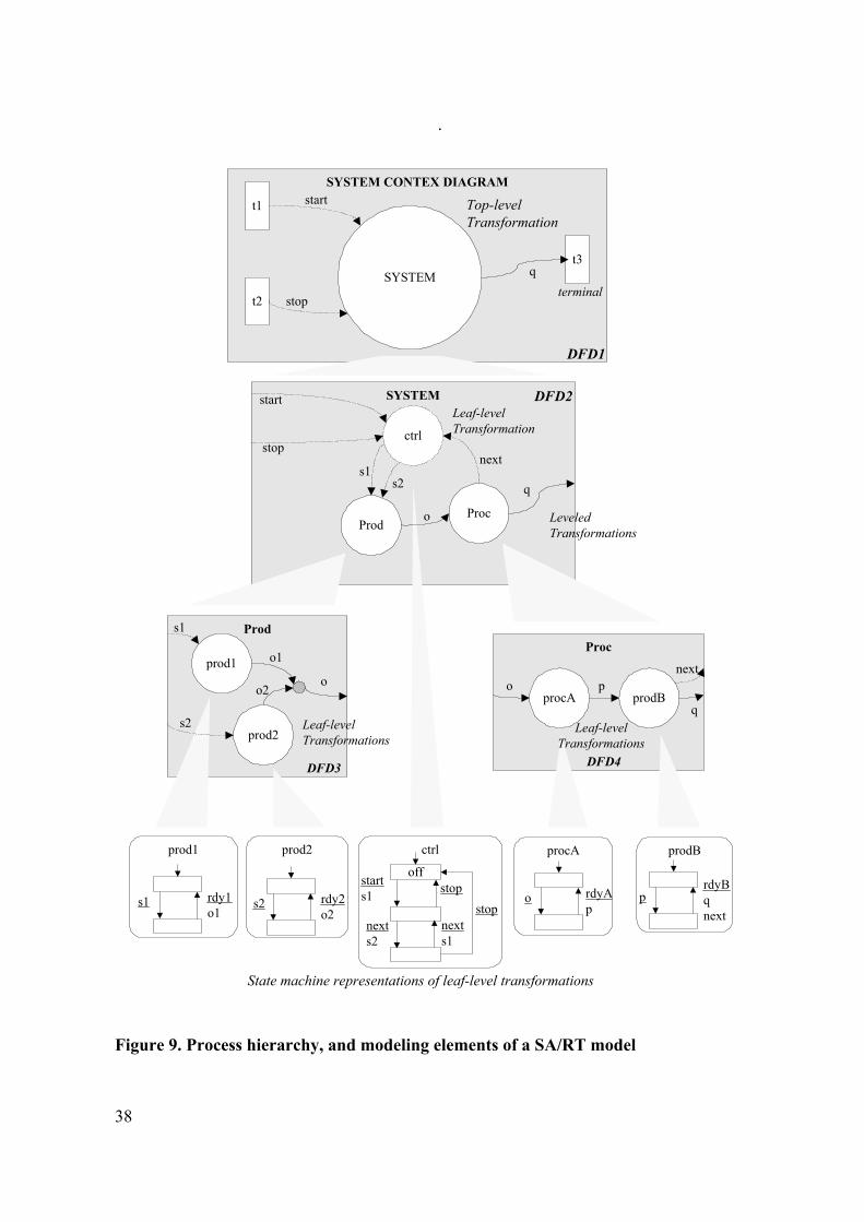
38
.
Prod
SYSTEM CONTEX DIAGRAM
prod1 prod2 ctrl procA prodB
s1 rdy1o1
offstarts1
nexts2
nexts1
stopstop
prdyBqnext
o rdyAp
SYSTEM
ctrl
ProdProc
Procprod1
procA prodB
prod2
oo
o1
o2 p
q
next
s1
s2
start
stop
s1s2
next
o
q
LeveledTransformations
Leaf-levelTransformations
Leaf-levelTransformation
Leaf-levelTransformations
State machine representations of leaf-level transformations
SYSTEM
t1
t3
t2
q
start
stop
Top-levelTransformation
s2 rdy2o2
DFD1
DFD2
DFD3 DFD4
terminal
Figure 9. Process hierarchy, and modeling elements of a SA/RT model
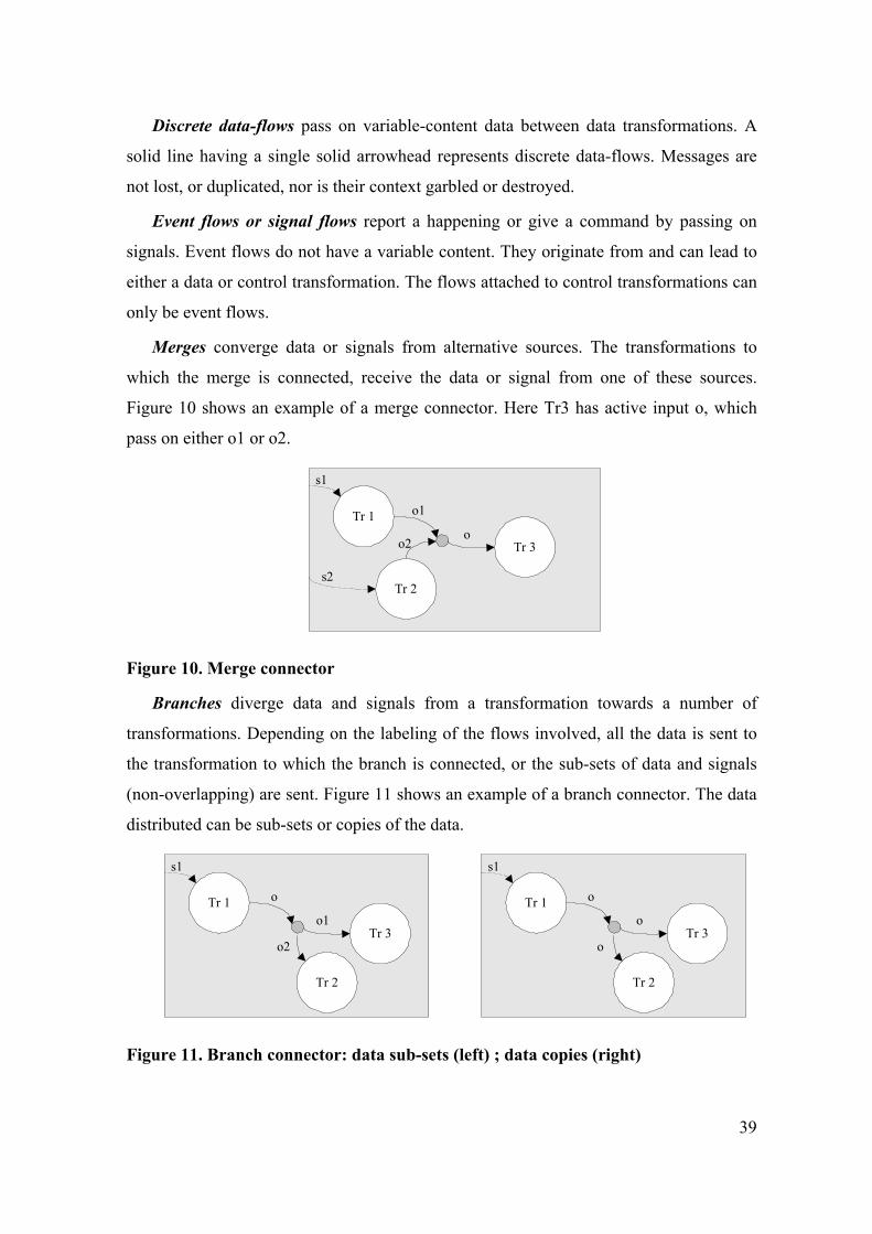
39
Discrete data-flows pass on variable-content data between data transformations. A
solid line having a single solid arrowhead represents discrete data-flows. Messages are
not lost, or duplicated, nor is their context garbled or destroyed.
Event flows or signal flows report a happening or give a command by passing on
signals. Event flows do not have a variable content. They originate from and can lead to
either a data or control transformation. The flows attached to control transformations can
only be event flows.
Merges converge data or signals from alternative sources. The transformations to
which the merge is connected, receive the data or signal from one of these sources.
Figure 10 shows an example of a merge connector. Here Tr3 has active input o, which
pass on either o1 or o2.
Tr 1
Tr 2
o
o1
o2
s1
s2
Tr 3
Figure 10. Merge connector
Branches diverge data and signals from a transformation towards a number of
transformations. Depending on the labeling of the flows involved, all the data is sent to
the transformation to which the branch is connected, or the sub-sets of data and signals
(non-overlapping) are sent. Figure 11 shows an example of a branch connector. The data
distributed can be sub-sets or copies of the data.
Tr 1 o
s1
Tr 3
Tr 2
o1
o2
Tr 1 o
s1
Tr 3
Tr 2
o
o
Figure 11. Branch connector: data sub-sets (left) ; data copies (right)

40
Data Stores are temporary placeholders for data and represent “transmission in time”
(as opposite to “transmission in space”). Data placed in stores are not changed. Pairs of
parallel straight-line segments graphically represent data stores. Transformations that
write or load the data are always associated with stores. Their interconnections are
depicted by a directed data-flow (non-solid arrow) from the transformation to the store,
and vice versa. The use of stores does not determine the causal relations between the
transformations. Note the difference with discrete data-flows. Data-flows pass on data
between stores and transformations, and vice versa; data-flows do not cause state any
transitions. This is in contrast to discrete data-flows. Figure 12 shows a data store and
data-flows for passing on data between Tr1 and Tr2. Data-flows do not cause any state
transitions, for this reason Tr2 is activated indirectly via an intermediate transformation,
in this case Ctrl.
Tr 1
s1
Ctrl
Tr 2
s2 s3
d
d
s4
Figure 12. Data store and data-flows
The notion of active inputs and active outputs are of importance for the SA/RT model
behavior. An active input arrives independently of any action of the receiving
transformation and starts the execution of the receiving transformation. An active output
is created by the activity of a transformation, and can be active input for another
transformation. The transformation’s inputs and outputs form its alphabet. Note that
inputs from and outputs to data stores are not considered to be active.
Data transformations always have one active input. An active input can originate
from the system’s environment or from another data or control transformation. Using the
merge element the active input can possibly originates from alternative sources. A data
transformation can also have an event flow as active input. In this case the data
transformation is given the command to start its execution and generate output, using

41
data that is for example stored in a data buffer. A data transformation can thus either
have a discrete data-flow or an event flow as active input.
A data transformation can have zero or more active outputs. An active output is a
discrete data-flow to a data transformation, or a signal to a data transformation or control
transformation. Data transformations possibly have alternative mode of executions with
different results and different sub-sets of active outputs that are generated. The
generation of multiple active outputs takes place concurrently.
The flows attached to control transformations are between transformations or
between a transformation and terminal only. The flows to and form control
transformations are event or signal flows only and do not have variable content data.
Each control transformation is embodied by a state machine, which involves states
and transitions. A transition is defined by the (current) state from which it emanates, the
(next) state it leads to, the guard (arrival of an particular active input) and outputs. That
is, for the transitions that possibly emanates from the current state, if one of their guards
becomes valid (the matching input becomes active), the transition takes place, the
outputs are generated and the transition next state becomes the state machine’s next state.
Data transformations involve execution time delays. The outputs are generated upon
receiving the active input, but only after some delay. The delays are non-deterministic
but greater than zero execution. Transitions in control transformations take place in
(virtual) zero delay. Also, no delays are involved with merges and branches.
2.4 Labeled Transition Systems
In the research reported in this thesis an approximate behavior is attached to the
SA/RT model for behavioral analysis, by specifying state machines for the primitive
processes and connectors. The state machines are defined as labeled transition systems
(LTS). The construction of state machines and the use of LTS execution rules for the
state machines give a formal base to the approximate behavior of the SA/RT model.
Labeled transition systems offer a formal framework that facilitates behavioral analysis.
The causal relations between system actions in the transition systems, reflect the causal
relations of corresponding actions in the SA/RT model.
State machines for the primitive processes (leaf level transformations) and connectors
can be constructed in a straightforward manner. Individual LTS’s are defined for each of

42
the state machines. The composition of the individual LTS’s defines the joint behavior of
all the leaf level transformations and connectors. Actions that belong to different
transition systems are synchronized if they have the same label. The composition
operator for labeled transition systems is used to construct the composite transition
system that represents the joint behavior of the individual state machines.
The composition of a number of component transition systems is realized by
operating directly on the component transition systems. The parallel composition
operator || , which is similar to the one in CSP, is hereby used. The composition operation
and independence relation computation can however be simplified if the transition
systems are first converted into a more suitable internal representation. This internal
model representation is discussed in a subsequent section.
The usual execution rules for the labeled transition systems are given first. A
transition system consists of a set of states, including an initial state, and transitions
between the states. The transitions’ labels represent the system actions. Transitions with
the same labels are synchronized.
Definition 1. Transition System A transition system is a structure ( , , , )T S i L Tran= where
• S is a set of states with the initial state i ,
• L is a set of labeled action that can be observed, and
• Tran S L S⊆ × × is the transition relation.
Let ( , , , )T S i L Tran= be a transition system. Then 'a
s s→ indicates that ( , , ')s a s Tran∈ .
Occasionally the notation /a
s → is used to indicate that there is no transition ( , , ')s a s .
The arc notation can be extended to string of labels 1 2 nv a a a= … , and v
ns s→ . The
string v is possibly an empty string of labels in L . The notation v
ns s→ is shorthand for
1 2
1 2
naa a
ns s s→ → →… for some states 1, ns s… . Let s i= and 'v
s s→ for some string v , then
the state 's is called a reachable state.

43
The execution of the labeled transition system ( , , , )T S i L Tran= is a possibly infinite
sequence 0 0 1 1..s a s a of states is and actions ia such that 0s i= and 0j∀ ≥ ,
( )1, ,j j js a s Tran+ ∈ .
Let ( , , , )T S i L Tran= be a labeled transition system. Transition system T is
deterministic if and only if for all , ', '' , s s s S∈
( ) ( ), , ' , , '' ' ''s a s Tran s a s Tran s s∈ ∧ ∈ ⇒ = , otherwise it is non-deterministic.
An action a L∈ is enabled at the state Ss ∈ , if and only if Ss ∈∃ ' such that
( , , ')s a s Tran∈ . Similarly, a transition ( , , ')s a s Tran∈ is enabled at a state St ∈ if and
only if st = . The idle transition ( , , )s s∗ indicates inaction. The execution rules for
transitions systems are given below.
aat t→
(2.1)
t t
∗
→ (2.2)
The parallel composition operator || is a binary operator. Let 0 0 0 0 0( , , , )T S i L Tran= and
1 1 1 1 1( , , , )T S i L Tran= be two transition systems. The composed transition system
( )0 1||T T T= is defined as follows. Let ( , , , )T S i L Tran= , and
• 0 1S S S= ×
• 0 1L L L= ∪
• 0 1' ' 'Tran Tran Tran Tran= ∪ ∪
• ( ) ( )( ) ( )( )
0 0 00 1 0 1
1 1 1
, , '' , , , ', '
, , '
s a s TranTran s s a s s
s a s Tran
⎧ ⎫∈ ∧⎪ ⎪= ⎨ ⎬∈⎪ ⎪⎩ ⎭
• ( ) ( )( ) ( ){ }0 0 1 0 1 0 0 0 1' , , , ', , , 'Tran s s a s s s a s Tran a L= ∈ ∧ ∉
• ( ) ( )( ) ( ){ }0 0 1 0 1 1 1 1 0' , , , , ' , , 'Tran s s a s s s a s Tran a L= ∈ ∧ ∉
The composed transition system 0 1T T T= satisfies the following execution rules.
( ) ( )
0 0 1 10 1
0 1 0 1
', ' ||, ', '
a a
a
s s s s T Ts s s s
→ →
→ (2.3)
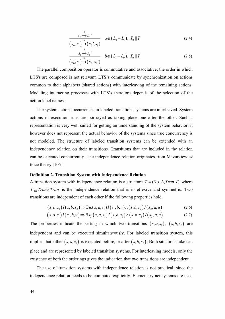
44
( ) ( )
( )0 00 1 0 1
0 1 0 1
' , ||, ',
a
a
s s a L L T Ts s s s
→∈ −
→ (2.4)
( ) ( )
( )1 11 0 0 1
0 1 0 1
' , ||, , '
b
bs s b L L T T
s s s s
→∈ −
→ (2.5)
The parallel composition operator is commutative and associative; the order in which
LTS's are composed is not relevant. LTS’s communicate by synchronization on actions
common to their alphabets (shared actions) with interleaving of the remaining actions.
Modeling interacting processes with LTS’s therefore depends of the selection of the
action label names.
The system actions occurrences in labeled transitions systems are interleaved. System
actions in execution runs are portrayed as taking place one after the other. Such a
representation is very well suited for getting an understanding of the system behavior; it
however does not represent the actual behavior of the systems since true concurrency is
not modeled. The structure of labeled transition systems can be extended with an
independence relation on their transitions. Transitions that are included in the relation
can be executed concurrently. The independence relation originates from Mazurkiewicz
trace theory [105].
Definition 2. Transition System with Independence Relation A transition system with independence relation is a structure ( , , , , )T S i L Tran I= where
I Tran Tran⊆ × is the independence relation that is ir-reflexive and symmetric. Two
transitions are independent of each other if the following properties hold.
( ) ( ) ( ) ( ) ( ) ( )1 2 1 1 2 2, , , , . , , , , , , , ,s a s I s b s u s a s I s b u s b s I s a u⇒ ∃ ∧ (2.6)
( ) ( ) ( ) ( ) ( ) ( )1 1 2 1 2 2 2, , , , . , , , , , , , ,s a s I s b u s s a s I s b s s b s I s a u⇒ ∃ ∧ (2.7)
The properties indicate the setting in which two transitions ( )1, ,s a s , ( )2, ,s b s are
independent and can be executed simultaneously. For labeled transition system, this
implies that either ( )1, ,s a s is executed before, or after ( )2, ,s b s . Both situations take can
place and are represented by labeled transition systems. For interleaving models, only the
existence of both the orderings gives the indication that two transitions are independent.
The use of transition systems with independence relation is not practical, since the
independence relation needs to be computed explicitly. Elementary net systems are used
45
as internal representation instead for modeling system behavior with true concurrency.
This way the limitations posed by transition systems are circumvented.
2.5 Labeled Net Systems
Net systems are used as an underlying model for the transition systems to represent
the system behavior as given by the SA/RT models. The net systems form the base
structure for obtaining the composite system behavior. A net system involves places,
transitions, and a flow relation connecting the places with transitions. Labeled net
systems are net systems that are extended with a labeling function :T L→ , which
attaches the system action names to the transitions of the net system. The structure of
labeled net systems is defined as follows. It extends the structure of net systems, which
definition is given in Appendix A.
Definition 3. Labeled Net System A labeled net system is given by the structure ( ), , ,N P T F= where ( ), ,P T F is a net
system, and :T L→ is a function that attaches a system action to each transition. The
set L contain the system actions.
The set P contain the places or conditions; the set T contains the transitions. The set
X P T= ∪ contains the elements (of N ), and F represents the flow relation (of N ). In
order to avoid confusion the notations NP , NT , NX and NF are sometimes used. The
notion ( ){ },F x x y F= ∈dom and ( ){ },F y x y F= ∈ran represent the relation domain
and range of F respectively.
For each x X∈ , ( ){ },Nx y X y x F• = ∈ ∈ is the input-set (or pre-set) of x ;
( ){ },Nx y X x y F• = ∈ ∈ is the output-set (or post-set) of x . The set x x• •∪ is called the
neighborhood of x , and denoted by ( )xnbh . In order to indicate the net under
consideration the notation ( )N
x• , ( )N
x• , and ( )N xnbh will be used. For Y X⊆ , the
notations x Y
Y x• •
∈= ∪ , and
x YY x• •
∈= ∪ and ( )Y Y Y• •= ∪nbh is carried over.
A net ( ), ,N P T F= can be seen as a directed graph NG where the nodes of NG are
the elements of X and there is an edge for x to y if and only if ( ),x y F∈ . Typically,
46
the P -elements are graphically depicted as boxes, T -elements are depicted as circles,
and the elements of the flow relation as arcs. The transitive closure F + indicates the
directed paths in NG ; the reflexive transitive closure F ∗ indicates (possibly empty)
directed paths in NG .
As discussed above, for a SA/RT model, the modeling elements’ approximate
behavior (data and control transformations, branches and merges) is represented by state
machines. The global system states and global system state transitions are distributed.
The joint approximate system behavior is the composite of the state machines. Global
system states are combinations of the machines’ local states; the system state transitions
are composed of the local state machine transitions. The state machines themselves in
turn are represented by the net systems. The net systems execution rules define the way
states machines cooperate. The net systems configurations represent the global system
states.
Graphically, a configuration C P⊆ is represented by a “token” placed in every place
of C . The transitions in T - represent atomic state changes. The flow relation F models
the relation between the conditions and events of a system. Since the net is marked with
tokens, a configuration is also referred to as a marking of the net.
Definition 4. Configuration A configuration of a net system ( ), ,N P T F= is a subset of P .
Elementary net systems are net systems for which an initial configuration (marking) is
given.
Definition 5. Elementary Net System An elementary net system is given by the structure ( ), , , inN P T F C= , where
( ), ,P T F is a net, and inC P⊆ is the initial configuration.
Labeled elementary systems have an additional labeling function :T L→ defined. The
labeled version of an elementary net system is given by the definition below.
Definition 6. Labeled Elementary Net System A labeled elementary net system is given by the structure ( ), , , , inN P T F C= , where
( ), , ,P T F is a labeled net system, and inC P⊆ is the initial configuration.

47
Configurations change as transitions take place. Let ( ), ,N P T F= be a net system, with
configurations C P⊆ , 'C P⊆ and t T∈ . The notation 't
C C→ indicates that the
occurrence of transition t causes C to change to 'C . For the elementary net systems,
states are also referred to as cases and transitions are referred to as steps. The places that
are affected by a transition are those that are directly preceding and succeeding it.
Definition 7. Pre- and Post-Conditions Let ( ), ,N P T F= be a net, , 'C C B⊆ and t T∗∈ . Transition t occurs at C if all the pre-
conditions, and none of the post-conditions of t hold. That is 't
C C→ if t C• ⊆ and
't C• ⊆ and \ '\C t C t• •= . The transitions , 't t T∗∈ are independent if and only if
( ) ( )' 't t t t• • • •∪ ∩ ∪ = ∅ .
Definition 8. Concession Let N be a net with markings C , 'C and transition t . Then '
tC C→ if and only if
t C• ⊆ , t C• ∩ = ∅ and ( )' \C C t t• •= ∪ .
Transition t has concession at C , that is t Ccon , if all its pre-conditions and none of its
post-conditions hold. The marking resulting from the occurrence of a transition is
determined by its pre- and post-sets. When t takes place at C the pre-set of t cease to
hold and the post-set of t becomes valid. The characteristic pair
( ) ( ) ( )', ' ,t C C C C t t• •= − − =cp gives the amount of change caused by t .
2.6 Causal Nets
Causal nets represent the unfolding of an elementary net system. The unfolding
represents a finite part of a system execution run. A causal net renders the system
execution trace of transitions taking place in combination with the conditions involved.
The causal net places and transitions are copies of the elementary net system conditions
and transitions. The following notions are related to the causal nets.
Definition 9. Partially Ordered Set Let A be a finite set. The binary relation A Aρ ⊆ × is a partial order on A , if ρ is ir-
reflexive and transitive. Then ( ),A ρ is a partially ordered set.
Notations that indicate the part before, and after an element set, and the initial and final
part of a partial ordered set are given below.

48
Definition 10. Before, After, Initial Final part Let ( ),A ρ be a partially ordered set and B A⊆ .
• ( ) ( ) ( ){ }. ,B a A b B a b a bρ
ρ↓ = ∈ ∃ ∈ ∈ ∨ = denotes the part of A before B
(including B ).
• ( ) ( ) ( ){ }. ,B a A b B b a a bρ
ρ↑ = ∈ ∃ ∈ ∈ ∨ = denotes the part of A after B
(including B ).
• ( ) ( ){ }' . ',B b B b B b bρ
ρ= ∈ ∃ ∈ ∈ denotes the initial part of B .
• ( ) ( ){ }' . , 'B b B b B b bρ
ρ= ∈ ∃ ∈ ∈ denotes the final part of B .
Causal nets are defined as follows.
Definition 11. Causal Net A net system ( ), ,M P T F= is a causal net if and only if it is a cycle-free and its
conditions do not have branches. The causal net comprises the partially ordered set
( ),MX F + .
( ) ( ).# 1 # 1Mp P p p• •∀ ∈ ≤ ∧ ≤ (2.8)
( ) ( )Mx y X x y F y x F+ +∀ ∈ ∈ ⇒ ∉, . , , (2.9)
Elements in a partial ordered set that are causal dependent have a line relation; elements
that can occur concurrently have a concurrency relation.
Definition 12. Line and Concurrency Relation Let ( ),A ρ be a partially ordered set. The line relation liρ of ρ is the binary relation for
,a b A∈
( ) ( ) ( ), iff a b a b b a a bρ ρ ρ∈ ∈ ∨ ∈ ∨ =, li , , (2.10)
The concurrency relation coρ of ρ is the binary relation for ,a b A∈
( ) ( ) ( ), iff a b a b b a a bρ ρ ρ∈ ∉ ∧ ∉ ∨ =, co , , (2.11)
Two distinct elements of A are either involved in liρ or in coρ . If a b= then
( ), lia b ρ∈ and ( ), coa b ρ∈ hold simultaneously.

49
Definition 13. Lines and cuts Let A be a finite set, and B A⊆ . Let A Aσ ⊆ × be a similarity relation (i.e. a relation
that is reflexive and symmetric). Then B is a σ -clique if ( ),a b σ∈ for all ,a b B∈ . B
is a maximal σ -clique if B is a σ -clique and for every a A B∈ − there exists b B∈
such that ( ),a b σ∉ . For the partially ordered set ( ),A ρ , a maximal liρ -clique is a line
and a maximal coρ -clique is a cut.
A causal net is used to represent the unfolding of an elementary net system. The
places in the causal net correspond to the places in the elementary net system. The
conditions in the causal net refer to conditions in the elementary net system. Condition
labeling functions can be associated with a causal net; they render the elements relation
of the two net systems.
Definition 14. Labeled Causal Net A labeled causal net is given by the structure ( )1 2, , , ,M P T F φ φ= , and ( ), ,P T F is the
underlying net system. The functions 1:P Pφ → Σ 2:T Pφ → Σ maps the places and
transitions of M to the set of elements 1Σ and 2Σ respectively.
Definition 15. Causal Net for System Run Let ( )1 2, , , ,M M MM P T F φ φ= be a labeled causal net and let ( )( ), , ,N N N in N
N P T F C= be a
contact-free elementary net system. Then M is a causal net for a system run of N if
1 2 and N NP T= =Σ Σ (2.12)
( ) ( )1 in NM Cφ = (2.13)
( ) ( )( ) ( ) ( )( )1 2 1 2 and t t t tφ φ φ φ• •• •= = (2.14)
( ) ( ) ( )( ), , for all ,M N Mx y F x y F x y Xφ φ∈ ⇒ ∈ ∈ (2.15)
The causal net’s firing sequences correspond to the firing sequences of their
corresponding elementary net system. Let ( )( ), , ,N N N in NN P T F C= be a contact-free
elementary net system, 1' ' 'nr t t= … be transitions in T , and ( )1
'ntt
in NC C→ →… , then
there exists a causal net ( )1 2, , , ,M M MM P T F φ φ= for N with transitions 1 nr t t= … such
that ( ) 'i it tφ = , for 1 i n≤ ≤ , ( ) ( )in NM Cφ = , ( ) 'M Cφ = and
1 ntt
M M→ →… .
For the mapping and scheduling decision, a number of system runs are selected that
represent typical system behavior or expose the system’s bottlenecks. These system runs
50
are the starting point for making the mapping and scheduling decision. They can be
represented separately or combined into one structure.
Event structures form a structure with which a number of execution runs can be
modeled. Let the set Evt denote the events of the system runs. Events possibly precede
one another, or are in conflict. The event structure ( ), ,EvtS Evt prec cnfl renders the
events, their precedence and their conflict relations.
Event structures are constructed by combining the causal nets of a number of system
runs can into one causal net, which includes conflicts. Conflicts are conditions in the
causal net that have multiple emerging transitions. Before the conflict, the system runs
exhibit the same behaviors hence their causal nets are the same; they however progress
differently after the conflict. Net elements that succeed elements that are in conflict are
in conflict too. Let ( ), ,P T F denote the causal net with conflicts that represent the
combined system runs. Its event structure is constructed as follows.
Evt T= (2.16)
( ) ( ){ }, ' , ' , 'prec e e e e F e e Evt+= ∈ ∧ ∈ (2.17)
( ) ( ) ( ){ }* *, ' , '. ' , ', 'confl x x t t t t t x F t x F• •= ∃ ∩ ≠ ∅ ∧ ∈ ∧ ∈ (2.18)
In this thesis, system runs are associated with use cases and represented by their event
structure.
2.7 Net System Operators
This section discusses the net system operator for constructing the composite system
from component systems. The definition uses a number of auxiliary notions and
definitions that are first being introduced.
Definition 16. Idling Transition Let ( ), ,N P T F= be a net system with transitions T , and ∗ denotes the undefined or
idling transition. The set T∗ is defined as { }T T∗ = ∪ ∗ , and ( )• ∗ = ∅ , ( )•∗ = ∅ .
Let T and T ' be sets. The product × of T and T ' is defined as
( ){ }T T t t t T t T× = ∈ ∈' , ' , ' ' . The specialized multiplication operator ∗× also considers
the idle transitions.
51
Definition 17. Specialized Multiplication For sets that include the idling transition, the operator ∗× is defined as
'T T∗× = ( ){ } ( ){ } ( ) ( ){ }, , ' ' , ' , ' 't t T t t T t t t t T T∗ ∈ ∪ ∗ ∈ ∪ ∈ × .
Projection functions for products render the individual participants of the
multiplication operation.
Definition 18. Projection The projections T T T Tπ × →: ' and T T T Tπ × →' : ' ' take the pair ( )t t T T∈ ×, ' ' to t
and 't respectively. The notation 0π , and 1π is also used and express projections onto
the first set involved in the multiplication and second set, respectively.
The disjoint union operation is introduced in order to combine the places of
component net systems.
Definition 19. Disjoint Union The disjoint union of two sets P and P ' is defined as
( ){ } ( ){ }' ,1 ', 2 ' 'P P p p P p p P= ∈ ∪ ∈ . The injection maps for disjoint unions is
defined as P P P Pµ →: ' with ( ) ( )1P p pµ = , , and ( )( )1 1P p pµ − =, , and
P P P Pµ →' : ' ' with ( ) ( )2P p pµ =' ' ', , and ( )( )1 2P p pµ − =' ', ' . The notation 0µ and 1
0µ − are also used to denote the operations related with the first set; 1µ and 11µ − is used to
denote the operations related with the second set.
The product of two net systems is a net system that is constructed as follows:
Definition 20. Product of Net Systems Let ( )0 0 0 0, ,N P T F= and ( )1 1 1 1, ,N P T F= be nets. Let 0 1N N N= × denote the net systems
product and ( ), ,N P T F= , with
• 0 1P P P= ,
• 0 * 1T T T= × ,
• ( )( ) ( )( )0 0 1 1t t tµ π µ π• • •= ∪
• ( )( ) ( )( )0 0 1 1t t tµ π µ π• •• = ∪
Similarly, the product of two elementary net systems is an elementary net system that is
constructed as follows:

52
Definition 21. Product of Elementary Net Systems Let ( )( )0 0 0 0 0
, , , inN P T F C= and ( )( )1 1 1 1 1, , , inN P T F C= be elementary net systems. Their
product 0 1N N× is given by the elementary net system ( ), , , inN P T F C= , and
• ( ) ( ) ( )0 0 0 1 1 1, , , , , ,P T F P T F P T F= ×
• ( ) ( )0 10 1in in inC C Cµ µ= ∪ .
The pair of maps ( )0 0π µ, specifies how the behavior of the product 0 1N N× projects to
the behavior of its component net system 0N . Similarly ( )1 1,π µ maps the net systems
product to component net system 1N .
2.8 Abstract Communication
The communication scheme used for the system architecture, set systems apart. The
schemes impose certain rules on the way communication actions actually take place. For
instance, the number of participating processes in a communication action, or the
buffering scheme used to implement a communication action renders different system
behaviors. The more constraints there are, the more specific the communication scheme
is. Ideally, this specificity comes with benefits. For instance, the more specific a
communication scheme is, the more straightforward it is to implement. The
communication mechanisms used in the system model for behavioral analysis determine
which mechanisms can be chosen for the communication actions in the implementation
model.
The distributed systems model of Charron-Bost et.al. [22] is used in this thesis for
conveying the possible communication schemes and their differences. In this model, a
distributed system consists of processes 1, , nP P… , communicating only by exchange of
messages. Message passing actions are represented by the individual send and
corresponding receive actions that are distributed over a sending and receiving
process(es) respectively. Communication is considered to be asynchronous; synchronous
communication is considered to be an asynchronous communication with additional
constraints. The occurrences of the send and receive actions take place at specific points
in time. On such a level of abstraction, space-time diagrams can be used to graphically
depict the distributed system’s execution runs. Herein, time moves from left to right,
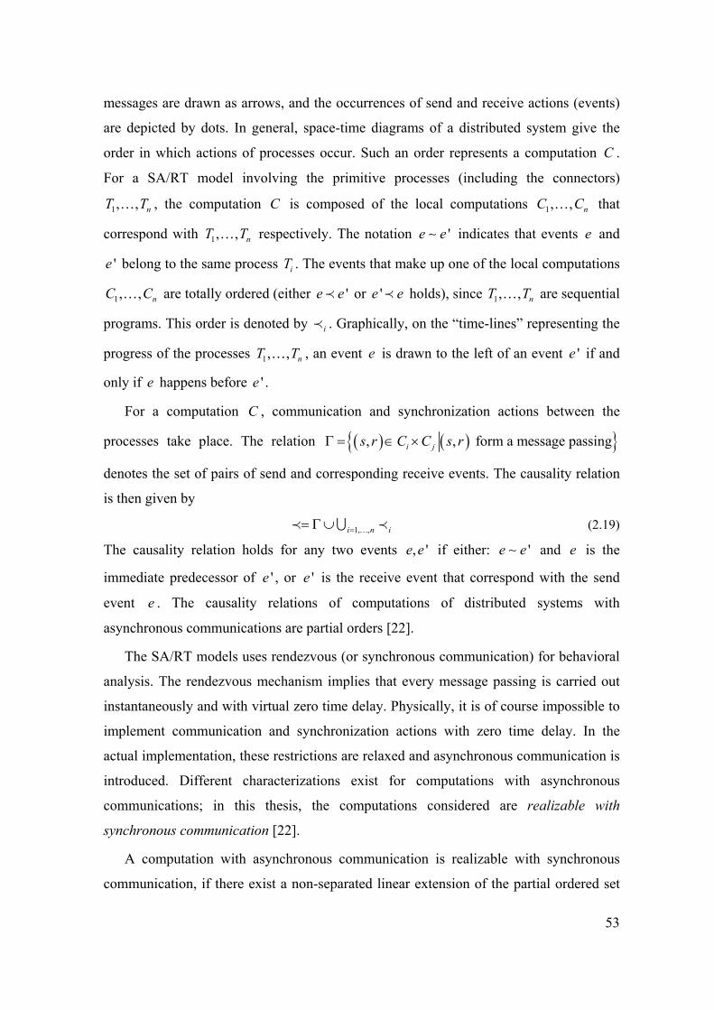
53
messages are drawn as arrows, and the occurrences of send and receive actions (events)
are depicted by dots. In general, space-time diagrams of a distributed system give the
order in which actions of processes occur. Such an order represents a computation C .
For a SA/RT model involving the primitive processes (including the connectors)
1, , nT T… , the computation C is composed of the local computations 1, , nC C… that
correspond with 1, , nT T… respectively. The notation 'e e∼ indicates that events e and
'e belong to the same process iT . The events that make up one of the local computations
1, , nC C… are totally ordered (either 'e e≺ or 'e e≺ holds), since 1, , nT T… are sequential
programs. This order is denoted by i≺ . Graphically, on the “time-lines” representing the
progress of the processes 1, , nT T… , an event e is drawn to the left of an event 'e if and
only if e happens before 'e .
For a computation C , communication and synchronization actions between the
processes take place. The relation ( ) ( ){ }, , form a message passingi js r C C s rΓ = ∈ ×
denotes the set of pairs of send and corresponding receive events. The causality relation
is then given by
1, ,i n i== Γ ∪ …≺ ∪ ≺ (2.19)
The causality relation holds for any two events , 'e e if either: 'e e∼ and e is the
immediate predecessor of 'e , or 'e is the receive event that correspond with the send
event e . The causality relations of computations of distributed systems with
asynchronous communications are partial orders [22].
The SA/RT models uses rendezvous (or synchronous communication) for behavioral
analysis. The rendezvous mechanism implies that every message passing is carried out
instantaneously and with virtual zero time delay. Physically, it is of course impossible to
implement communication and synchronization actions with zero time delay. In the
actual implementation, these restrictions are relaxed and asynchronous communication is
introduced. Different characterizations exist for computations with asynchronous
communications; in this thesis, the computations considered are realizable with
synchronous communication [22].
A computation with asynchronous communication is realizable with synchronous
communication, if there exist a non-separated linear extension of the partial ordered set
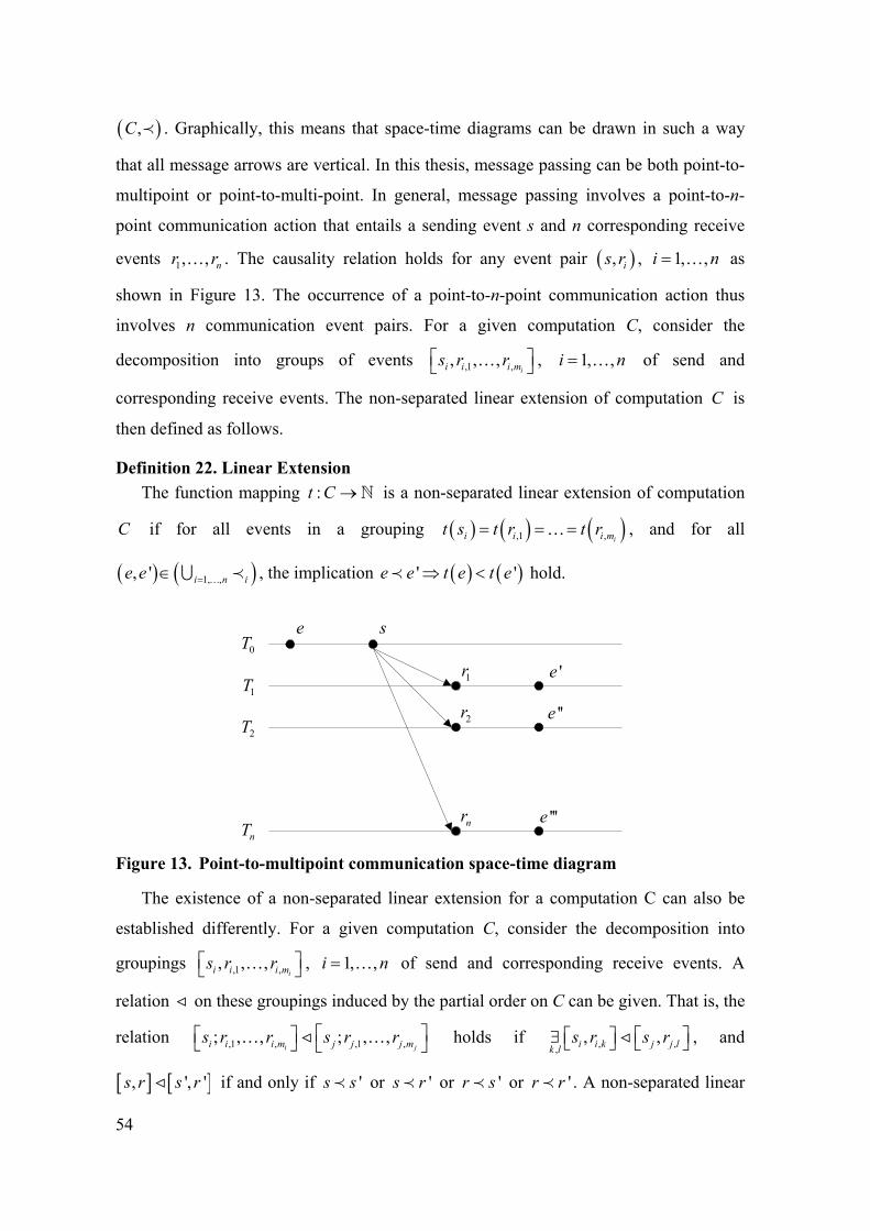
54
( ),C ≺ . Graphically, this means that space-time diagrams can be drawn in such a way
that all message arrows are vertical. In this thesis, message passing can be both point-to-
multipoint or point-to-multi-point. In general, message passing involves a point-to-n-
point communication action that entails a sending event s and n corresponding receive
events 1, , nr r… . The causality relation holds for any event pair ( ), is r , 1, ,i n= … as
shown in Figure 13. The occurrence of a point-to-n-point communication action thus
involves n communication event pairs. For a given computation C, consider the
decomposition into groups of events ,1 ,, , ,ii i i ms r r⎡ ⎤⎣ ⎦… , 1, ,i n= … of send and
corresponding receive events. The non-separated linear extension of computation C is
then defined as follows.
Definition 22. Linear Extension The function mapping :t C → is a non-separated linear extension of computation
C if for all events in a grouping ( ) ( ) ( ),1 , ii i i mt s t r t r= = =… , and for all
( ) ( )1, ,, ' i n ie e =∈ …∪ ≺ , the implication ( ) ( )' 'e e t e t e⇒ <≺ hold.
e s
1r1T
0T
2T
nT
2r
nr
'e
''e
'''e
Figure 13. Point-to-multipoint communication space-time diagram
The existence of a non-separated linear extension for a computation C can also be
established differently. For a given computation C, consider the decomposition into
groupings ,1 ,, , ,ii i i ms r r⎡ ⎤⎣ ⎦… , 1, ,i n= … of send and corresponding receive events. A
relation on these groupings induced by the partial order on C can be given. That is, the
relation ,1 , ,1 ,; , , ; , ,i ji i i m j j j ms r r s r r⎡ ⎤⎡ ⎤⎣ ⎦ ⎣ ⎦… … holds if , ,,
, ,i i k j j lk ls r s r⎡ ⎤⎡ ⎤∃ ⎣ ⎦ ⎣ ⎦ , and
[ ] [ ], ', 's r s r if and only if 's s≺ or 's r≺ or 'r s≺ or 'r r≺ . A non-separated linear

55
extension only exists if and only if the set of groupings of send and corresponding
receive events, together with the relation , form a partial order. That is, let + be the
transitive closure of . Then ,1 , ,1 ,. , , , , , ,i ii i i m i i i mi s r r s r r+⎡ ⎤ ⎡ ⎤∃/ ⎣ ⎦ ⎣ ⎦… … ; there are no directed
cycles.
The space-time diagram for a computation with asynchronous communication is
equivalent with that for computations with synchronous communication [22]. The causal
relations for computations with asynchronous communication that is realizable with
synchronous communication, can be obtained by behavioral analysis of its counterpart
with synchronous communication

56
57
Chapter 3.
Decision-Making for System Design
3.1 Introduction
System design is best organized as an evolutionary quality engineering process [79].
The alternatives for a system design problem and the system architect’s preferences
concerning the compromise to choose are not an objective reality and need first to be
constructed by stepwise refinements and possibly iterations. The objectives involved are
typically incommensurable and in conflict with each other. Also, assessments of criteria
can often only be given in qualitative terms and are thus imprecise. The problem setting
in system design as briefly described above is to some extent similar to that addressed by
Multiple-Criteria Decision Making (MCDM) as considered by decision theory (e.g. [124]
[143]). MCDM is however not an approach that is typically used for solving system
design problems; the problem setting for MCDM as considered by decision theory is
somewhat different from the one by quality-driven design decision-making. Also, system
design problems involve additional aspects that are not dealt with directly by MCDM. By
identifying the similarities in their problem settings, system design decision-making can
benefit from certain MCDM concepts and methods.
In the following sections, the most important differences and concerns that are not
dealt with directly by MCDM are passed in review. Basic MCDM notions and methods
are discussed. MCDM usually makes a distinction between multi-attribute decision-
making (MADM) and multi-objective optimization problems (MOOP). In the quality-
driven decision-making processes, preferences are specified progressively. The
representation used to model preferences and organization of the decision-making
process, are to some extent similar to that of interactive methods in MOOP. Whereas
58
MOOP typically makes use of mathematical programming techniques, system design
problem solving deploys heuristic search, since system design problems are typically
combinatorial optimization problems that are NP-hard. Mathematical programming
techniques as used in MOOP are often not suited for these problems.
System design problem solving makes use of heuristic search. Another aspect, which
benefits from MCDM is modeling and solving the selection, ranking, or sorting problem
of alternative (intermediate) solutions and search directions. In this thesis, the heuristics
search is equipped with multi-criteria decision-making aids. In particular MADM
methods are used to sort the intermediate solutions during search. The heuristic search is
implemented using genetic algorithms; an overview of the genetic algorithms meta-
heuristics is given and specific procedures are identified for which the deployment of
MADM methods is considered desirable.
3.2 MCDM for Quality-driven Design Decision-Making
The quality engineering process basically starts with an abstract, imprecise,
incomplete and possibly contradictory initial model of the required quality (initial
requirements) and transforms the initial model into a concrete, precise, complete
coherent and final model that can be implemented. The quality engineering process is
evolutionary and it consists of generating the tentative quality models, using them for
constructing, selecting and improving of the tentative solutions, analyzing and estimating
them directly and through analysis of the resulting solutions, changing them and using
them again etc. The initial model is more abstract and usually involves some behavioral
and parametric characteristics and to a lesser extent, the structural characteristics. The
final model defines the system's structure completely and explicitly. This structure
supports the required system's behavior and fulfills the parametric requirements in a
satisfactory manner. The well-structured models of the required, proposed or delivered
design quality serve to enable well-organized design decision making with open and
rational procedures, to enable design automation etc. The design-time reduction due to
automation will enable more extensive exploration of the model and design-spaces, and
leading to designs of higher quality.
The design process resolve on comprise solutions does not come about easily, since
the set or continuum of solutions is not an objective reality and does not simply exist.
59
The solutions need to be constructed first and possibly lack important aspects since they
are an idealization of the actual problem. Moreover, there is incomplete information
about the decision maker's preferences; usually, the decision maker only has an idea
about preferences with regard to some concrete solutions rather than a complete picture
of the preferences space; in this thesis, "what if" analyses are used to complete this
picture. Another reason for the information incompleteness is the imprecision with which
the criteria are assessed. Crisp data may simply be non-obtainable due to the high costs
involved, or assessments can only be given as qualitative data, such as linguistic
qualifications. Approximations for the criteria values are then given instead; the
decision-making methods deployed need to be able to represent and handle these
imprecise assessments.
Some of the most important concerns that are additional, and differences between the
quality-driven design decision-making process and the MCDM process as considered by
decision theory are the following. MCDM typically considers either a limited set of
alternatives, or a continuous solution space that is described and searched using single
objective linear and non-linear mathematical programming techniques. The solution
space typical for system design issues is however discrete and the sets of alternatives are
very large or infinite. In contrast to the alternatives in MCDM, the alternatives in system
design are unknown a priori and cannot be exhaustively enumerated and evaluated. A
limited number of the most promising alternatives must be constructed during the design
process and this construction has to be guided by decision models. Also, the decision
models of MCDM as discussed by decision theory rely too often on the availability of
knowledge of well-established preferences of the decision-maker that is representative
for the whole design space. In system design, the system architect must build the
preference model by analyzing the design problem or sampling the design space parallel
to dealing with the system design issues. The decision models in design are tentative and
are subject to further design and change. They are considered to be heuristics for setting
and controlling the course of design.
System design decision-making can benefit from certain MCDM concepts and
methods by identifying the similarities in their problem settings. Multiple-Criteria
Decision Making is both an approach for organizing the decision making process, as well
as a collection of facilitating techniques. The system design process can, similar to the
60
MCDM process, be organized in a model-based manner. The process then relies on
models that adequately represent the decision situations. This implies that the model can
be used for predicting and evaluating the consequences of decisions. For an
optimization-based decision making process, the models can also be used to compute
decisions that would attain the specified goals or maximizes the objective function.
Multi-criteria decision-making can also be applied in system design, in the frame of
heuristic search for solutions that are satisfactory. The information available to rank, sort
or select search directions is typically weak for making conclusive and unambiguous
decisions. In the case of a constructive search, it is used to select the most promising
construction operators and partial solutions. Therefore, in design, the decision models
should not only be constructed for the complete solutions, but also for partial solutions
and construction operators of a certain issue. In the case of parallel search, multi-criteria
decision-making is not only used to select the most promising solutions but also to
guarantee the diversity of the solution population. Here it is typically not straightforward
how to make the tradeoffs and take all the issues into account. System design can benefit
from MCDM methods for sorting and ranking sets of alternatives, and from methods for
modeling the system architect preferences in the frame of heuristic search and
optimization.
3.3 MCDM methods
3.3.1 Basic Notions
MCDM traditionally considers two types of problem settings: the multi-attribute
decision-making (MADM) problems, and the multi-objective optimization problems
(MOOP). Whereas multi-attribute decision-making problems involve a limited number
of alternatives that are given explicitly, the alternatives in multiple objective optimization
problems are implicitly enumerated or the number can be infinite. The solutions for
MOOP are specified by constraint functions or constraints in short, and thus given in a
declarative manner.
The multi-attribute decision problem setting is described as follows. It addresses the
problem setting in which the set 0X of alternatives needs to be sorted or ranked, or a
solution 0X∈x needs to be chosen. The vector x involves the decision variables that

61
represent the solution. Furthermore, a consistent family F of criteria has been specified
for 0X .
• The sorting problem divides 0X into subsets according to some norm.
• The ranking problem ranks the alternatives in 0X from best to worst.
• The choice problem determines a subset of alternatives that are considered the
best with respect to F .
The Multiple Objective Optimization Problem is traditionally given as a mathematical
programming model. Whereas 0X is given explicitly for MADM problems, it is
enumerated or given implicitly for MOOP. For MOOP, 0X renders the space of
admissible solutions and involves a number of constraint functions. Similar as for
MADM problems, for a MOOP a consistent family F of criteria is also specified for
0X .
Definition 23. Multiple Objective Optimization Problem (MOOP)
The MOOP include a set of decision variables and is the problem of simultaneously
minimizing the m criteria or objective functions , i 1, ,if m= … . Objective functions and
constraints are functions of the decision vector x . The optimization goal is to
( ) ( ) ( )( )( ) ( ) ( )( )( ) ( ) ( )( )
1
1
1
minimize , ,
subject to , ,
, ,
k
k l
l m
f x f x
g x g x
h x h x+
+
= =
= ≥
=
0
= 0
…
…
…
y f x
g x
h x
(3.1)
and ∈x X , ∈y Y where X is the decision space, and Y is the objective space. The set
of admissible solution is given by
( ) ( ){ }0 = ∈ ≤ =0, 0X x X g x h x (3.2)
The functions :ig →X R , 1, ,i k l= + … , and :jh →X R , 1, ,j l m= + … are the
constraint functions. The image of 0X , that is the feasible region in the objective space is
denoted as ( )0 0=Y f X .
The decision maker can freely choose the values for the decision variables as long as
they comply with the constraint functions specified. This is in contrast to the indicator
and other auxiliary variables in the model; their values are determined by the values of

62
the decision variables or other indicator and auxiliary variables. The notions below give
some characterizations of alternatives, how alternatives relate to each other and of crucial
points in the objective space.
Definition 24. Dominance Relation
The dominance relation “alternative x dominates y ” ( Dx y ) is defined as
( ) ( ) ( ) ( )
{ }1, , 1, ,
i i j jjD q q q q
i m j m
⇔ ≥ ∧ ∃ >
= ∈… …
x y x y x y (3.3)
Definition 25. Efficient Solution
The solution 0X∈x is efficient if and only if it is not being dominated by another
solution in 0X .
Definition 26. Pareto-optimal Front
The set 0Y X⊆ is the Pareto-optimal front if and only if
0 ,Y X
D∈ ∈ ≠∀ ∃/y x x y
x y (3.4)
Definition 27. Ideal Point
The ideal or utopia point is the point ( )* *1 , , mq q… in the objective space, and
( )0
* maxi iXq q
∈=
xx .
Definition 28. Nadir Point
The nadir point is the point ( )1, , mq q… in the objective space, and ( )0
mini iXq q
∈=
xx .
Definition 29 . Aspiration Point
An aspiration point (or reference point) is composed of the values for each criterion
desired by the decision maker. The aspiration point is defined as mq ∈R .
Definition 30. Reservation Point
A reservation point is composed of the values still acceptable by the decision maker for
each criterion. The reservation point is defined as mq ∈R .

63
3.3.2 MCDM Model-Based Process
The multi-criteria decision making process is model-based; it involves the models
0X and F that represent the alternatives and preferences respectively. The
representation of the problem setting is not an objective reality, for which an immediate
description can be given that is accepted by everyone. The same real-life problem may
imply
• different definitions of 0X
• different definitions of F
• different statement of the problem (minimization, goal attainment, sorting etc.).
It is practical to divide the specification and generation of a MADM and MOOP
model into two stages. In the first stage the core model is specified and generated. The
core model involves the set of variables and constraints that define the set or continuum
of admissible solutions 0X . The core model involves the logical and structural relations
that hold for the admissible solutions.
In the second stage, the preference model F is specified, which includes the decision
maker’s preferences, and goals such as the objectives’ values that the decision maker
wants to achieve or avoid. The specification of the preference model possibly results in
the generation of additional constraints and variables, which are then added to the core
model. The number of additional constraints and variables is a small fraction of what is
already included in the core model.
3.4 Multi-Attribute Decision-Making Methods
The following multi-attribute decision-making methods are distinguished in this
thesis.
• Utility / Multi-Attribute Value Theory (MAVT) [148]
• Aspiration-based methods [101] [122]
• Outranking methods [124] [125]
• Non-compensatory methods [143]

64
3.4.1 Utility Functions
In MAVT methods (or utility methods), the decision maker provides a mathematical
value function : mU →R R relating all m objectives. The value function must be valid
over the entire decision space containing all the feasible alternatives. It renders the utility
each criterion provides, and the interactions among the different criteria. The value
function is a complete pre-order. That is, for two solutions x and y , either
( ) ( )U U≥x y or ( ) ( )U U≤x y holds. The MAVT combines multiple objectives into a
single-objective function that can be used for classical search and optimization
techniques.
The MAVT is a straightforward model for representing the decision maker
preferences. The requirements to appropriately use the MAVT are however high. The
decision maker needs to be able to specify a value function, which is applicable over the
entire decision space. This implies, for instance, that the decision maker needs to be able
to determine the trade-offs between all the criteria in the model. This is feasible for
criteria that can be converted into monetary units. For more abstract criteria, these trade-
offs are however often difficult to determine.
An additional difficulty for using MAVT is that the correlation between the criteria
needs first to be resolved. The dependencies that exist between the criteria determine
which aggregation scheme can be used for the value function. For instance, the additive
weighting scheme can only be used if the criteria are independent of each other.
Otherwise, the value function has a multiplicative or mixed form.
MAVT objective functions are compensatory, and assume that large amount of trade-
off information can be elicited from the decision maker. If this requirement cannot be
met then the value function constructed is possibly an oversimplified model of the
decision maker preferences. Because the constructed value function determines the
solution obtained in MOOP and MADM, the oversimplification possibly results in a
solution that is not the actual preferred one.
3.4.2 Aspiration-Based Methods
In order to be able to solve MADM and MOOP problems with less trade-off
information required from the decision maker, alternative methods have been proposed
in literature [143]. Aspiration-based methods are an alternative to MAVT for specifying

65
the decision maker preferences. The decision maker specifies the goals (or negative-
goals) for one or more criteria that need to be attained. The solutions that minimize or
maximize the deviations from these goals are the preferred solutions.
The TOPSIS method is an example of such a multi-attribute decision-making
method. It uses goals for specifying the decision maker’s preferences. In TOPSIS the
ideal and nadir points are used as reference points. The preferred solution is the solution
that has the shortest distance from the ideal solution and the farthest from the nadir point.
The distance function is specified according to some norm.
Goal programming is an example of a MOOP optimization method that uses goals to
specify the decision maker’s preferences. The goals are used to construct a single-
objective function. The single-objective optimization problem in goal programming has
the following form
( ) ( )( )
1
1
0
minimize ,
subject to
,
m kk
i i ii
h q q q q
q q qX
α+ − + −
=
+ −
+ −
⎛ ⎞= +⎜ ⎟
⎝ ⎠+ − =
∈≥
∑
0
f xx
q q
(3.5)
Here 0iα > and the function ( ),h q q+ − is the weighted k -norm of the difference
( ) q−f x . The variables iq+ and iq− are the overachievement respectively
underachievement of the i -th criterion. For example, if the set 0X is described by linear
inequalities, the function f is linear, and for the 1 -norm is used then a linear
programming problem is obtained.
Aspiration-based methods are a further development and generalization of goal
programming [101] [122]. Goal programming methods generate solutions that are closest
to the goal. They however not necessarily generate Pareto-efficient solutions that
maximize a monotonous utility function. This is in contrast to aspiration-based methods.
Aspiration-based methods use so-called achievement functions that are a certain class of
utility functions, which when maximized, produces Pareto-efficient solutions with regard
to the multiple objectives.
The decision maker’s preferences are specified by means of aspiration levels that
determine the solution generated. Aspiration levels have the advantage that the decision
66
maker can easily modify them and test their attainability. This way the decision maker
gets an understanding of the admissible and Pareto-efficient solutions.
Let ( )1, , mq q q= … represent the aspiration point specified by the decision maker.
Individual utility functions are first specified that describe the decision maker regret or
disutility when the actual outcome falls below the aspiration, or the utility for reaching
more than the aspiration level for a particular criterion. For example, if the utility for
reaching the aspiration level is set to, e.g. 0.9, then the following utility function
describes the decision maker preferences.
,max
,min
0.9 0.1 if
0.9 0.9 if
i ii i
i ii
i ii i
i i
q q q qq q
q q q qq q
µ
−⎧ + >⎪ −⎪= ⎨ −⎪ − <⎪ −⎩
(3.6)
The achievement function ( ),s q q is the composite of the individual utility function
1, , mµ µ… and can be given as:
( )1
, min ii ms q q µ
≤ ≤= (3.7)
This particular achievement function is not strictly monotonous with respect to the
decision outcomes ( )i iq f= x . More sophisticated aggregation schemes that have more
favorable characteristics are discussed in [101].
3.4.3 Outranking Methods
MAVT and achievement functions can both be used for MADM and MOOP. MOOP
however requires that the preference model be in the form of a single-objective function.
Preferences modeling methods, which only target MADM problems, are not bound to
this requirement. Therefore, for MADM, preferences models can also be specified in
terms of procedural steps that need to be undertaken in order to select, sort or rank a set
of alternatives.
Outranking methods only address MADM problems. Instead of specifying the
ordering between all the alternatives, the decision maker specifies an outranking relation
between pairs of alternatives (relative to a criterion); the total order for the solutions is
not constructed. The outranking relations indicate the strength of preference of one
alternative over the other one. The strength of preferences between alternatives is given
by indices.

67
The concordance index ( ),c x y for the alternatives x and y takes a value between
zero and one and gives the arguments in favor of the statement x outranks y . Each
criterion iq is assigned a weight iα . The relative weight of a criterion is added to the
index if x outranks y for that particular criterion. That is
( )( ) ( ):
1
1, .j j
jj q qi
i m
c αα ≥
≤ ≤
= ∑∑ x yx y (3.8)
If the concordance index is larger than the concordance threshold c the concordance
relation Cx y holds. That is:
( ) ˆ,C c c⇔ ≥x y x y (3.9)
In order to be completely certain that x is preferred over y , the values of y should not
exceed that of x by a large margin for all the criteria. If this is the case then the
discordance relation Dx y holds.
( ) ( ) ( )i
,max ,min
max i i
i i
q qd
q q−
⇔−
y xx, y (3.10)
( ) ˆD d d⇔ ≥x y x, y (3.11)
The outranking relation between the alternatives x and y holds, if only their
concordance relation and not their discordance relation are active.
P C D⇔ ∧ //x y x y x y (3.12)
The outranking relation can be represented as a graph. The degrees of the graph’s
vertices can be used as measures to rank the alternatives. Vertices that have more
outgoing edges are alternatives that have more outranking relations than vertices with
less outgoing edges. A higher rank is assigned to these vertices. Similarly, vertices that
have more incoming edges are assigned a lower rank than vertices with less incoming
edges.
The most basic outranking method involves one concordance and one discordance
threshold. Refinements for outranking methods can be introduced by using multiple
concordance thresholds. Instead of one concordance relation, multiple relations that
indicate increasing outranking strengths are distinguished. For example, for two
thresholds, a strong and a weak outranking relation are distinguished.
Outranking methods requires less information than MAVT. The amount of
information that needs to be obtained from the decision maker can however still be
68
considerable, especially when the criteria involved have a high level of abstraction.
Weights need to be assigned to the criteria and the thresholds need to be defined for the
concordance and discordance relations. This information pertains to the inter-criterion
trade-offs the decision maker is willing to make.
3.4.4 Non-Compensatory Methods
In order to decrease the amount of trade-off information needed from the decision
maker, one can resort to non-compensatory methods. For example, the lexicographic
method is a non-compensatory method. It requires an ordering of the criteria in terms of
their importance. For m , and k m≤ criteria, if the first 1k − criteria renders
( ) ( ) , 1, , 1i iq q i k= = −…x y , then the decision maker only considers the first k criteria.
Using the lexicographic methods, the preference of alternative x over y is defined as
follows.
( ) ( ) ( ) ( ) ( ), , and , 1, , 1k k i iP q q q q i k> = = −…x y x y x y (3.13)
The dominance method is another non-compensatory method for sorting a set of
alternatives. The sub-set of non-dominated alternatives forms the Pareto-optimal front of
the set of alternatives. The dominance method sorts the alternatives into Pareto-efficient
fronts by repeatedly screening out the non-dominated ones. At each step, the non-
dominated alternatives are assigned a higher rank than the dominated ones. In the next
step, the screening procedure is repeated for the dominated alternatives. The method is
completed if the set to be screened only contains non-dominated solutions. The
alternatives in this set are then assigned the lowest rank. The dominance method is also
referred to as the non-dominated sorting method.
3.5 Multi-Objective Optimization Problems
Multi-objective optimization problems involve more than a single objective. These
objectives are typically conflicting and are possibly incommensurable. Whereas, for
multi-attribute decision-making problems, the alternatives are explicitly given and their
number is finite, for multi-objective optimization problems the alternatives are given or
enumerated implicitly by constraint functions. For these reasons, a process for modeling
the MOOP and selecting a suitable compromise solution is needed.
69
MOOP methods can be grouped according to the approach adopted for organizing the
decision-making process. Three classes of process organization are typically
distinguished for MOOP [31], and also adopted in this thesis. As discussed above,
MCDM is model-based and typically two conceptually distinct phases are distinguished:
the analysis phase and the decision making phase. In the analysis phase the core model is
specified. The analysis phase is pre-dominantly occupied with generating the model that
represents the alternatives. Objectives and preferences are specified in the decision
making phase.
A priori articulation of preferences (a priori methods) - The decision-making process
starts with the construction of a composite single objective function based on the
decision maker’s preferences. The objective function is then used to determine the
optimal solution in the decision space of admissible solutions.
MAVT is typically associated with this class of methods. As discussed earlier the
amount of information that needs to be specified is considerable, and the use of MAVT is
only possible when the decision maker is able to provide sufficient information for
constructing the value function. For these reason other means for specifying the decision
maker’s preferences that require far less information are used in this thesis. The
specification of preferences takes place in terms of goals in this thesis.
Progressive articulation of preferences (interactive methods) - The decision-making
process takes place progressively, that is the analysis and decision-making phase take
place interactively. Instead of a priori constructing the composite single objective
function for generating the solutions, the preferences are specified tentatively in order to
sample the solution space. Also the preferences are specified in terms of goals; the solver
then finds the efficient solution closest to the reference point.
The characteristics of interactive methods are different than those for a priori
methods. Whereas the latter methods construct the composite single objective function
first, the decision-making process for interactive methods takes place progressively. The
decision-making process involves a learning process in which objectives, criteria,
constraints, alternatives and preferences continually interact and redefine each other; the
process then leads to a satisfactory solution. Besides the variations of goals, constraints
or objective weights can be varied for generating other efficient solutions and sample the
solutions space.
70
A posterior articulation of preferences (posterior methods) - A posterior methods
adopt a completely different approach for organizing the decision-making process. The
decision-making process starts with an extensive analysis phase in which investigations
are undertaken to generate the complete set or entire continuum of possible efficient
alternatives. It is followed by the decision making phase in which the decision maker
inspects the set or continuum of proposals, clarifies his preferences in terms of a
preference function and makes a choice. Pareto-optimal solutions can be obtained by
variations of constraints, weights or reference points according to some procedure.
3.6 Decision-Making for System Design
MOOP are usually solved using single-objective linear and non-linear mathematical
programming techniques. The field of search and optimization has however changed
over the past decade by the introduction of a number of non-classical, stochastic search
and optimization algorithms. Of these, the genetic algorithm (GA) is used in this thesis.
A genetic algorithm mimics nature's principles to drive its search towards an optimal
solution across generations. GA transition rules are, in contrast to the rules for classical
optimization techniques, probabilistic and not deterministic. Theoretically GA’s
converge to the optimal solutions; in practice however there is no guarantee that GA’s
converge to the optimal solution. GA are used to generate compromise solutions for the
MOOP’s.
Genetic algorithms differ in a number of important aspects from linear and non-linear
mathematical programming techniques for MOOP. These mathematical programming
techniques are referred to as classical methods in this thesis. Mathematical programming
techniques make use of linear and non-linear constraint functions to represent the
admissible solutions; GA’s can also make use of problem-specific genetic
representations to model the problem setting. In particular procedural specifications can
be used to construct solutions. Also, the search direction for classical optimization
methods is determined by both the (derivatives of the) objective function and the
constraints that define the admissible decision space. GA’s in contrast, make only use of
the payoff information for determining the search direction; the GA search direction is
determined by the landscape of the objective space only.

71
The classical methods are single-objective optimization methods; the decision
maker’s preferences need first to be combined into a single objective function, in order to
solve the MOOP. The use of derivative information however limits the aggregation
scheme that can be used to relatively simple ones. The choice is basically limited to
MAVT and goals, since these methods permit the construction of, and make available the
information concerning the derivatives of the composite single objective function from
the original ones. Because only the payoff information is needed for GA, basically all
multi-attribute decision-making methods can be used to model the decision maker
preferences pertaining to the search direction. The construction of decision models using
outranking methods and non-compensatory methods in particular require the least
amount of information from the decision maker. For this reason they are most suited to
be deployed at the early stages of design.
The decision-making for the evolutionary quality engineering process is organized
similar to the way interactive methods are organized in MCDM. The essence of the
iterative method assumed is summarized as follows: The decision maker selects, out of
the potential objectives, a number of variables that will serve as criteria for evaluations
of the feasible solutions 0x X∈ .
1. The decision maker specifies the aspiration level ( )1, , mq q= …q , and
corresponding utility functions.
2. If the optimization model is implemented as a mathematical programming
problem, then it first needs to be converted into one with a composite single-
objective. For MOOP, the aspiration points determine the achievement functions
that are used as composite objective functions.
3. Depending on the method used for search and optimization different aggregation
schemes can be used.
a. For classical optimization and search methods achievement functions are used
as composite single-objective function. The solution generated is a Pareto-
optimal point. If the aspiration point specified is not attainable, the solution is
the efficient solution that is the nearest to the aspiration level. If the aspiration
level is attainable, then the Pareto-optimal point is uniformly better than the
aspiration point q .

72
b. If the optimization model is implemented as a genetic algorithm, then the
individual component achievement functions (monotonously increasing utility
function) do not need to be aggregated into a composite single-objective
function. Other aggregation schemes, i.e. outranking and non-compensatory
methods, can now be used in order to specify the preference relation between
the alternatives.
4. The decision maker explores the objective space and decision space by specifying
various aspiration points and changing them. The solver selects or generates the
alternative that is closest to the aspiration point.
5. The procedures described in 2,3,4 are repeated until a satisfactory solution is
found.
3.7 Genetic Algorithms
3.7.1 Basic Principles
A genetic algorithm for a particular problem must have the following components
[108]:
• a way to represent potential solutions to the problem
• a way to create an initial population (these solutions preferably have high
potential)
• an evaluation function in order to rate the fitness of solutions
• a selection process for creating the next generation
• genetic operators, usually recombination and mutation, in order to diversify the
population
The solution candidates in genetic algorithms are called individuals and the set of
solution candidates is called the population. The set of all possible individuals form the
individual space I . The population is a multi-set of vectors i I∈ .
Individuals represent decision vectors. The relation between the decision variables
that form admissible solutions can be straightforward, or can be more complex. In the
latter case, decoders are used to compute the decision vectors that correspond with the
individuals that are not necessarily admissible in the decision space. The decoder thus
maps the individuals to their corresponding decision vectors. That is, given an individual

73
i I∈ , the mapping function d represents the decoding algorithm for computing the
decision vector ( )x d i= for the individuals i I∈ . The function f maps the decision
vector into a point in the objective space; the fitness is assigned based on the values of
this point. The individuals encode the decision vectors according to some appropriate
structure, such as a graph or an ordered list.
In the selection process, individuals that have high potential are to be reproduced;
individuals that are of low quality need to be removed from the population. This way
only the "fittest" individuals survive and reproduce their genetic information to the next
generation. The selection of the population for the next generation is supposedly to lead
the search to the best solution. Each individual is evaluated to give some measure for its
fitness. In early versions of the genetic algorithm, the quality of an individual with
respect to the optimization objectives (and constraints) is represented by a scalar value.
The genetic algorithm involves an iterative computation process. First, an initial
population is created. Then a number of generations are computed that is based on the
population of the previous iteration. For each iteration, the average quality of the
population increases. The best individual found across the generations is the outcome of
the genetic algorithm.
Let ( ) { }1 , ,t tNP t i i= … be the population of individuals that is distinguished at
iteration t . Each individual tji , { }1, ,j N∈ … is evaluated to give some measure of its
fitness (fitness assignment). Then, the more fit individuals are selected to form a new
population for iteration 1t + . Some members of this new population undergo alterations
by means of genetic operators. Genetic operators aim to generate new solutions within
the search space by the variation of existing ones.
• The crossover operator takes a certain number of parents and creates a certain
number of offspring by recombining the parents. Usually, a crossover probability
is associated with this operator.
• The mutation operator modifies an individual by changing small parts of its
structure. A mutation rate is associated with the operator.
Figure 14. gives the pseudo-code for genetic algorithms. The genetic algorithm involves
the parents and offspring populations. For generation t , they are denoted by ( )P t and
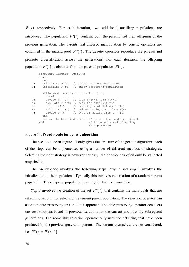
74
( )'P t respectively. For each iteration, two additional auxiliary populations are
introduced. The population ( )''P t contains both the parents and their offspring of the
previous generation. The parents that undergo manipulation by genetic operators are
contained in the mating pool ( )'''P t . The genetic operators reproduce the parents and
promote diversification across the generations. For each iteration, the offspring
population ( )'P t is obtained from the parents’ population ( )P t .
procedure Genetic Algorithm begin t=0 1: initialize P(0) // create random population 2: initialize P'(0) // empty offspring population while (not termination condition) do t=t+1 3: create P''(t) // from P'(t-1) and P(t-1) 4: evaluate P''(t) // rank the alternatives 5: select P(t) // take top-ranked from P''(t) 6: select P'''(t) // select mating pool from P(t) 7: create P'(t) // copy or modify from P'''(t) end render the best individual // select the best individual end // in parents and offspring // population
Figure 14. Pseudo-code for genetic algorithm
The pseudo-code in Figure 14 only gives the structure of the genetic algorithm. Each
of the steps can be implemented using a number of different methods or strategies.
Selecting the right strategy is however not easy; their choice can often only be validated
empirically.
The pseudo-code involves the following steps. Step 1 and step 2 involves the
initialization of the populations. Typically this involves the creation of a random parents
population. The offspring population is empty for the first generation.
Step 3 involves the creation of the set ( )'''P t that contains the individuals that are
taken into account for selecting the current parent population. The selection operator can
adopt an elite-preserving or non-elitist approach. The elite-preserving operator considers
the best solutions found in previous iterations for the current and possibly subsequent
generations. The non-elitist selection operator only uses the offspring that have been
produced by the previous generation parents. The parents themselves are not considered,
i.e. ( ) ( )''' ' 1P t P t= − .

75
In this thesis, the elite pre-serving operator is used. There exists a number of ways to
introduce elitism. In the simplest implementation, the n best parents and the popN n−
offspring of the previous generation parents form the current parents population. The
best solutions now get passed on directly from one generation to the other, and
participate in creating the offspring.
In this thesis the parents population ( )1P t − and the offspring population ( )' 1P t −
from the previous iteration are combined to form population ( )''P t . The popN best
solutions from ( )''P t need to be selected to form the parents’ population ( )P t . The
selection problem is solved using the enhanced version of the non-dominated sorting
method. The sorting method identifies a number of sorting bins: 1 2, ,B B … etc., which
contains the individuals that are equally ranked.
The combined population ( )''P t contains pop offspringN N+ individuals. The size of
parents population is however restricted to popN individuals. Only a subset of ( )''P t can
be included in ( )P t . Let 1 2 1m popB B B M N−+ + + = ≤… , 1 2 m popB B B N+ + + >…
then the best 1m − bins are included in the new population.
Application-domain criteria typically relates to individual alternatives. Besides
application domain criteria, genetic algorithms can make use of measures that indicate
the impact an individual has on the population in order to evaluate alternatives. The
individuals in bin mB are ranked according to their crowding distance. The crowding
distance gives a measure of the density of neighboring solutions that surrounds an
individual in the decision space, objective space or combination of spaces. It is discussed
in more detail in the next section. Besides application-domain criteria alternatives are
evaluated based on their contribution to a diverse population. The popM N− best-ranked
individuals from mB are selected to fill up the remaining places in the newly created
population.
Often a predefined maximum number of iterations are used as the termination
condition. The number of iterations and the size of the populations are limited and given
by the variable iterationsN . Other termination conditions used are, for example, the coming
76
to a stand still of the increase of the average quality or the existence of a solution that
meet some predefined quality level.
Theoretically, genetic algorithms are capable of rendering the best solution contained
in the individual space. In practice however, this cannot be guaranteed, since this
requires an infinite number of iterations and an unrestricted population size. Empirical
results however show that genetic algorithms have proven themselves as a general,
robust and powerful search mechanism and can in practice be used as meta-heuristics [5].
3.7.2 Crowding distance
In genetic algorithms, a stochastic selection process simulates the natural selection.
The population size is limited and given by the variable popN . Each solution is given a
chance to reproduce themselves a number of times, dependent on their quality. Two
aspects are of importance for the selection process to function properly. On one hand,
only those individuals that have high potential and that lead to the best solution are to be
selected. On the other hand however, the population need to be diverse in order to
prevent the algorithm to get stuck to only a small area in the individual space and/or
objective space. These considerations in particular apply for multi-modal optimization
problems that have multiple solutions that are local optima. For multi-modal
optimization problems, the convergence to a small area in the individual space and/or
objective space means that only one of many solutions above a certain threshold is found
and/or that the solution found is sub-optimal.
In order to guarantee the diversity of the population, a crowding distance can be used
[32]. The crowding distance of an individual gives the density of neighboring solutions
that surround the individual. It is used besides the application-domain specific criteria
and objectives for representing the fitness of the individuals. The crowding distance can
be given for the decision space and/or for the objective space. It can also be given for a
subset of the dimensions in these spaces.
Let j refer to the dimension or criteria in the decision space or objective space
respectively. The variable ( )jq i gives the level of quality of individual i for
dimension/criterion j . Let ( ),1 ,, ,j j j md d= …d , popm N= be a vector containing elements
that are sorted and are the quality levels of the individuals in the population. That is,
77
{ }( )( ) ( ), , , 12, , 1
. j l j j l j ll m i Id q i d d +∈ − ∈
∀ ∃ = ∧ ≤…
, with ,1 ,minj jd q= , , ,maxj m jd q= . Furthermore, for
i I∈ the following relationships are defined: ( ) ( ) ,j j j ld i q i d= = , ( )j i l= . The
crowding distance of i I∈ for the criterion j is defined as
( ) ( ) ( ), 1 , 1j j i j icd i d d+ −= − (3.14)
Let J be the set of criteria that define of interest. Then the crowding distance for an
individual i I∈ is defined by ( ) ( )j
j J
cd i cd i∈
= ∑ (3.15)
3.7.3 Selection Operator
The goal of the selection operator is to identify, make duplicates of solutions that
have high potential, and eliminate bad solutions in a population. There exists a number of
ways to achieve this goal. Some prevalent methods for the selection operator are, for
example, the proportionate selection operator, the ranking selection operator and the
tournament selection operator. The mating pool contains the copies of the individuals;
the higher the individual’s potential is the greater the number of copies in the mating
pool is.
In the proportionate selection method, solutions are assigned copies. The number of
the copies is proportional to their fitness values ( )q i , ( )i P t∈ . If the average fitness of
all population members is ( )( )
( )avgi P t
q q i P t∈
= ∑ , then a solution with fitness ( )q i gets
an expected ( ) avgq i q⎡ ⎤⎢ ⎥ number of copies. The selection of individuals into the mating
pool does not take place deterministically but stochastically. The selection takes place by
generating matingN random numbers within a certain range. Each individual is assigned an
interval on this range, which size is proportional to individual's fitness value. The
intervals are non-overlapping and contiguous. If for an iteration the generated random
number falls within a certain interval then the associated individual is selected into the
mating pool. This selection step is repeated matingN times.
The use of the proportionate selection method has some drawbacks. A solution with
fitness ( )q i gets an expected ( ) avgq i q number of copies in the mating pool. There is
however a large variance around the expected value each turn the method is being

78
applied. Selecting part of the mating pool in a deterministic manner, and part of it
stochastically reduces the variance.
Another more severe drawback that applies in particular applies for system design
problems, is that the proportionate selection method depends on the availability of a
single-objective utility function to represent the solutions’ fitness. The fitness values are
then used directly to determine the individual's probability of being selected in the
mating pool. The fitness values have to be given on a cardinal scale; the decision maker
has to specify the total order of the solutions and also need to be able to determine how
much better a solution is compared to another one. As discussed earlier, unless the
criteria can be translated into monetary units, the specification of such a utility function
is difficult and usually impossible in the early stages of design.
In order to get round the difficulty of determining a utility function, the solution’s
fitness is given on an ordinal scale. The ordinal scale is obtained by sorting the solutions
according their merits, from the worst (rank 1) to the best (rank N ). Each member in the
sorted list is assigned a fitness value equal to the rank of the solution in the list. The
probabilities for selection of the individuals into the mating pool are determined by using
these ranks as fitness values.
Both the proportionate method and the ranking method deploy probabilities, which
indicate the odds with which individuals are selected into the mating pool. The
tournament method is a method that does not require the computation of these
probabilities. It requires for this reason less trade-off information from the system
architect than the proportionate method or the ranking method. In the tournament
selection method, t solutions are randomly drawn from the population. An arbitrary
tournament size t can be chosen. The solutions drawn can be replaced or not. The
solutions drawn participate in a tournament, and the winning individual is inserted in the
mating pool. The process is repeated matingN times in order to create the new mating pool.
The winning individual can be determined based on some fitness value. The construction
of a single-objective utility function that represents the solutions’ fitness is however not
required. The winning individual can also be determined by comparing only the
participants in the tournament.
79
In this thesis the binary tournament selection operator is used for creating the mating
pool. Hereby two solutions are randomly drawn from the parents’ population. The
parents’ population has been sorted and the individuals have been grouped into sorting
bins. The sorting problem is solved using MCDM aids. The individual that belongs to a
higher ranked sorting bin wins the tournament and is inserted in the mating pool. The
individuals drawn are all re-inserted into the parents’ population; replacement takes
place. These steps are repeated matingN times, that is, matingN winning individuals are
inserted in the mating pool. In case the individuals that participate in the tournament
belong to the same sorting bin, then the individual that has the largest crowding distance
is designated as winner. If the crowding distances are the same then an individual is
selected randomly.
The selection operator does not create any new solutions in the mating pool; its intent
is only to make more copies of good solutions at the expense of not-so-good ones.
Crossover and mutation operators look after the creation of new solutions.
The crossover operation typically takes place by drawing two individuals from the
mating pool at random. Sub-structures of the individuals' structure are exchanged in
order to create two new solutions. In a single-point crossover operator one sub-structure
is identified and exchanged. A multi-point crossover operation involves multiple sub-
structures that are exchanged.
The way the crossover operates depends on the structure that is used to represent the
solutions. For example, for strings the single point crossover operator involves the
following. The cross operator draws pairs of individuals (parent solutions) from the
mating pool at random, which are not replaced. Sub-structures are identified within the
parent solutions, which are combined in order to create new solutions. For strings this
means that a crossing point is chosen at random for the first parent string. The crossing
point divides the parent string into a left and a right sub-string. It is assumed that the
individuals’ strings are of the same length. A crossing point in the second parent string is
inserted, which has the same position as the crossing point in the first parent string.
Recombining the sub-strings creates two new individuals. Combining the left sub-string
of the first parent with the right sub-string of the second parent forms the first new
individual. The second individual is formed using the parents’ sub-strings the other way
round.

80
The individuals that undergo the crossover operations are not any two arbitrary
random individuals. These individuals have survived tournaments in the process of
creating the mating pool. For this reason, it can be expected that the solutions in the
mating pool contain advantageous sub-structures. The advantageous sub-structures are
passed on to next generations. It is assumed that the combination of advantageous sub-
structures results in a solution that has a higher potential.
In order to preserve some good individuals in non-elitist approaches, not all the
newly created individuals are inserted in the offspring population. Either the newly
created solutions, or the unchanged parents are inserted in the offspring population. In
the latter case the parents are simply copied into the offspring population. The insertion
of the newly created solutions happens with the crossover probability of cp ; the parents
are inserted with a probability of 1 cp− . For elite-preserving methods the offspring and
their parents are mixed and evaluated together. This way it is assured that individuals
with high potential propagates and are not removed from the population by chance.
Additional to crossover, the mutation operator is used to ensure the diversity in the
population and search the decision space. The mutation operation only alters an
elementary part of the structure. For a bit string, the mutation operator randomly chooses
a bit and changes a zero to one, and vice versa. This happens with the probability of mp ,
which is the mutation probability.
3.7.4 Post-processing
The genetic algorithm can be used in combination with constraint satisfaction
problem solving techniques. The variables that describe a solution can often be divided
into sub-sets of related variables. The variables in the sub-sets possibly have different
impact on the criteria values. If this is the case then search can be organized in such a
way that first a global search is performed that renders an overall solution for which the
most determining decision variables are set. Post-processing is then used to refine the
solution, and repair possible constraint violations. Constraint satisfaction can be used for
implementing the post-processing step.
A constraint satisfaction problem is defined by a set of variables associated to
domains, and a set of constraints on these variables. Solving a constraint satisfaction

81
problem consists in finding assignments of all variables that satisfy all constraints. A
domain may be a continuous range, or an integer range, possibly enumerated.
An algorithm to search for a solution involves the reduction of each domain, one after
the other, until it either leads to a solution or fails to find one. Every time a value is
removed from a domain, the constraints acting on this domain are inspected to check if
any constraint causes that another value, belonging to another domain, becomes
forbidden. If so, it is removed too, and the process is recursively repeated. This is process
is called constraint propagation.
The domain reduction occurs then either by choice, or as consequence of the
propagation required for the satisfaction of some constraints. Upon failure (a domain
becomes empty), the algorithm backtracks to the last decision made, and takes the
opposite one, and tries again. If there is also no solution, the algorithm backtrack one
step further, and examine the stack of decisions bottom to top until either no solution or
one solution is found.
This is only the basic algorithm of the constraints satisfaction, however to this basic
algorithm various (problem specific) heuristics can be added that can make the total
algorithm much more sophisticated. The modern constraint satisfaction solvers enable
for many search strategies and relatively ease of supplementing them with extra
heuristics.

82

83
Chapter 4.
Behavioral Model
4.1 Approximate System Behavior
The approximate system behavior attached to SA/RT models are given in terms of
the state machines in the research reported in this thesis. State machines already specify
the control transformations. For behavioral analysis, the state machines that represent
data transformations, merges and branches need to be constructed additionally.
The transitions in these state machines represent some system action. The
transformations communicate and synchronize with each other using rendezvous or
shared actions for message passing. Message passing can be point-to-point or point-to-
multipoint in case branches are involved. The state machines have been introduced
above. The precise definition for their structure is given subsequently. .
Definition 31 State Machine The state machine structure is given by ( ), , , , ,SM S i T Tran A λ= . Where S denotes the
set of states distinguished for the data and control transformations; i S∈ is the initial
state; T is the set of transitions; Tran S T S⊆ × × is the set transition relation; A is the
set of system actions; and ( )( )T A Aλ ⊆ × ×P is the relation between transitions, the
action guarding the transitions or conditional action, and the set of actions resulting from
the transition.
The relation λ renders all state transitions. It consists of two component functions
0 T Aλ ⊆ × and ( )1 T Aλ ⊆ ×P . For all ( ), ,t a O λ∈ , propositions ( ) 0,t a λ∈ and
( ) 1,t O λ∈ hold. The guarded or conditional action a (active input) for transition t is
given by ( )0 tλ . The set of emerging actions (active output) for transition t is given by
84
( )1 tλ . State transition ( ), ,t a O λ∈ takes place if action a becomes active, after which
the outgoing actions O are carried out. The notation /a O
→ is equivalent to ( ), ,t a O λ∈ .
Rendezvous communication is assumed for behavioral analysis; action a becomes active
only if its counterpart is active too.
A state machine representation is attached to each SA/RT modeling element. The
construction of state machines for transformations, merges, branches and stores is
described below.
4.1.1 Data Transformation State Machines
The construction method for state machines representations for data transformations
is described below. The state machines are defined up to instantiation, which involves re-
labeling the states and state transitions (to obtain an isomorphic instance).
Discrete Data Transformations - The behavior of the discrete data transformations
DTR is represented by three states off, waiting, and active. The transformation has three
inputs: one activating input a, and the activating and deactivating inputs enable, and
disable respectively
Autonomous system actions are introduced for a transformation that indicates that its
execution is completed. There can be multiple system actions for a transformation, that
each indicates a different way of completion. Additional inputs represent each of these
system actions. Since they are autonomous, it appears as if they originate from the
system context. Let { }1, , nRdy rdy rdy= … denote the set of inputs that indicate the
completion of the transformation’s execution. The actions irdy , { }1, ,i ∈ … correspond
with the different ways the transformation can complete its execution. An example of the
state machine representation for a discrete data transformation is given in Figure 15.
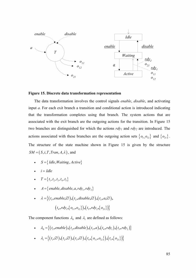
85
Ta
enable disable
o11o12
o21
Idle
Waiting
Active
a
enable disable
rdy1o11o12
rdy2o21
Figure 15. Discrete data transformation representation
The data transformation involves the control signals enable, disable, and activating
input a. For each exit branch a transition and conditional action is introduced indicating
that the transformation completes using that branch. The system actions that are
associated with the exit branch are the outgoing actions for the transition. In Figure 15
two branches are distinguished for which the actions rdy1 and rdy2 are introduced. The
actions associated with these branches are the outgoing action sets { }11, 12o o and { }21o .
The structure of the state machine shown in Figure 15 is given by the structure
( ), , , , ,SM S i T Tran A λ= , and
• { }, ,S Idle Waiting Active=
• i Idle=
• { }1 2 3 4 5, , , ,T t t t t t=
• { }1 2, , , ,A enable disable a rdy rdy=
• ( ) ( ) ( ){ 1 2 3t enable t disable t aλ = ∅ ∅ ∅, , , , , , , , ,
{ }( ) { }( )}4 1 11 12 5 2 21 t rdy o o t rdy o, , , , , ,
The component functions 0λ and 1λ are defined as follows:
• ( ) ( ) ( ) ( ) ( ){ }0 1 2 3 4 1 5 2t enable t disable t a t rdy t rdyλ = , , , , , , , , ,
• ( ) ( ) ( ) { }( ) { }( ){ }1 1 2 3 4 11 12 5 21t t t t o o t oλ = ∅ ∅ ∅, , , , , , , , , ,

86
Triggered Data Transformations – Triggered data transformations are activated by a
signal flow instead of a discrete data-flow. The method for constructing state machines
for triggered data transformations is described below. State machines are defined up to
instantiation, which involves re-labeling the states and state transitions. The behavior of
triggered data transformations DTR is represented by two states waiting, active. A
transformation has one activating input a. It involves autonomous system actions that
indicate that the transformation execution is completed, similar as for discrete data
transformations. There can be multiple system actions, that each indicates a different way
of completion. Additional inputs { }1, , nRdy rdy rdy= … represent these system actions.
An example of the state machine representation for a triggered data transformation is
given in Figure 16.
DTR
o11o12
o21
a
Waiting
Active
ardy1o11o12
rdy2o21
Figure 16. Triggered data transformation representation
4.1.2 Control Transformation State Machines
The state machines for control transformations are directly obtained from the initial
transformation specification. The control transformation's states and transitions map one-
to-one to those of the corresponding initial state machine.
4.1.3 Branches and Merges
The method for constructing the state machines for branches and merges is described
below. The state machines are defined up to instantiation, which involves re-labeling the
states and state transitions (conditional and set of emerging actions).
Branches - The behavior of branches BRNCH is represented by a single wait state. A
branch has one activating input a, and multiple outputs. Let O denotes these outputs, and
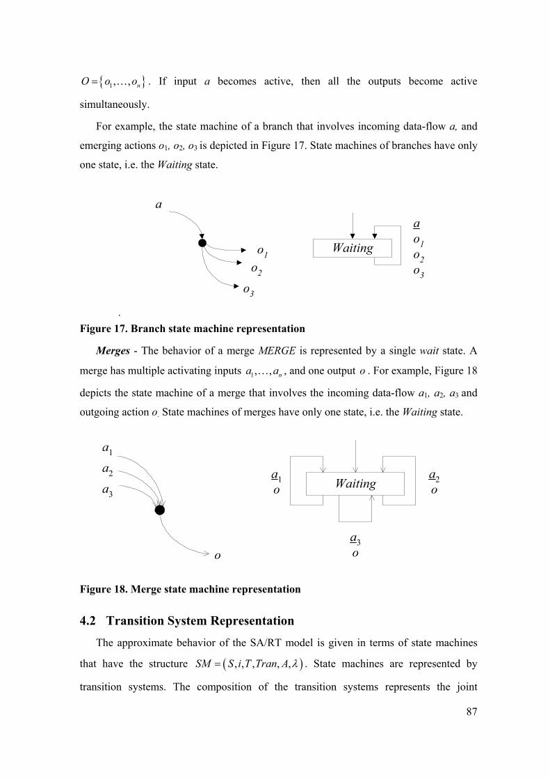
87
{ }1, , nO o o= … . If input a becomes active, then all the outputs become active
simultaneously.
For example, the state machine of a branch that involves incoming data-flow a, and
emerging actions o1, o2, o3 is depicted in Figure 17. State machines of branches have only
one state, i.e. the Waiting state.
.
a
o1o2
o3
Waiting
ao1o2o3
Figure 17. Branch state machine representation
Merges - The behavior of a merge MERGE is represented by a single wait state. A
merge has multiple activating inputs 1, , na a… , and one output o . For example, Figure 18
depicts the state machine of a merge that involves the incoming data-flow a1, a2, a3 and
outgoing action o. State machines of merges have only one state, i.e. the Waiting state.
Waiting
a1
a2
a3
o
a1o
a2o
a3o
Figure 18. Merge state machine representation
4.2 Transition System Representation
The approximate behavior of the SA/RT model is given in terms of state machines
that have the structure ( ), , , , ,SM S i T Tran A λ= . State machines are represented by
transition systems. The composition of the transition systems represents the joint
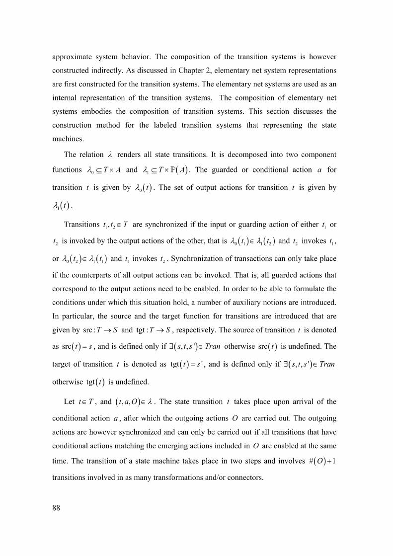
88
approximate system behavior. The composition of the transition systems is however
constructed indirectly. As discussed in Chapter 2, elementary net system representations
are first constructed for the transition systems. The elementary net systems are used as an
internal representation of the transition systems. The composition of elementary net
systems embodies the composition of transition systems. This section discusses the
construction method for the labeled transition systems that representing the state
machines.
The relation λ renders all state transitions. It is decomposed into two component
functions 0 T Aλ ⊆ × and ( )1 T Aλ ⊆ ×P . The guarded or conditional action a for
transition t is given by ( )0 tλ . The set of output actions for transition t is given by
( )1 tλ .
Transitions 1 2,t t T∈ are synchronized if the input or guarding action of either 1t or
2t is invoked by the output actions of the other, that is ( ) ( )0 1 1 2t tλ λ∈ and 2t invokes 1t ,
or ( ) ( )0 2 1 1t tλ λ∈ and 1t invokes 2t . Synchronization of transactions can only take place
if the counterparts of all output actions can be invoked. That is, all guarded actions that
correspond to the output actions need to be enabled. In order to be able to formulate the
conditions under which this situation hold, a number of auxiliary notions are introduced.
In particular, the source and the target function for transitions are introduced that are
given by src :T S→ and tgt :T S→ , respectively. The source of transition t is denoted
as ( )src t s= , and is defined only if ( ), , 's t s Tran∃ ∈ otherwise ( )src t is undefined. The
target of transition t is denoted as ( )tgt 't s= , and is defined only if ( ), , 's t s Tran∃ ∈
otherwise ( )tgt t is undefined.
Let t T∈ , and ( ), ,t a O λ∈ . The state transition t takes place upon arrival of the
conditional action a , after which the outgoing actions O are carried out. The outgoing
actions are however synchronized and can only be carried out if all transitions that have
conditional actions matching the emerging actions included in O are enabled at the same
time. The transition of a state machine takes place in two steps and involves ( )# 1O +
transitions involved in as many transformations and/or connectors.
89
Let jSM , 1, ,j m= … be the state machines that jointly give the system
representation. The set 1, ,
jj n
T T=
=…∪ contains all transitions of the system. The set ET
represents the subset of T that includes transitions that have output actions. The set ET ,
and the functions :Tη → , ( ) { }0 1: ,T Tσ × →P and ( ):T Tµ × →P are defined
as follows:
( )( ){ }1# 1ET t t T tλ= ∈ ∧ ≥ (4.1)
The function :Tη → assigns a transition system number to each transition. The
transitions that belong to the same state machine (i.e. same SA/RT modeling element)
are assigned the same number by η . The transitions that belong to different modeling
elements are assigned different numbers.
The function ( ) { }: 0,1T Tσ × →P is defined for transition - transition set pairs
( ) ( ),t st T T∈ ×P and indicates whether the output action of transition t can possibly
invoke the transitions in set st . The output actions of transition t are given by ( )1 tλ .
Transition t possibly invokes the transitions in st only if conditions listed below are
satisfied:
• the guarded actions of the transitions in st have labels that match the labels of
the output actions of t ,
• all output action of t are matched, and
• none of the transitions t and those included in st involve the same modeling
element (i.e. state machine).
The function ( )t stσ , depends on the value of its sub-functions ( ),t stρ and
( ),t stµ . The function ( ) { }0 1T Tρ × →: ,P specifies whether the input actions of
transitions in st have labels that match the output actions of t , and that all output actions
of t have been matched. This function is defined as follows:
( ) ( ) ( ) ( ){ }( ) ( )( )0 1 0 11 ' . ' # ' ' #,
0 otherwise
t st t t t t st tt st
λ λ λ λρ
⎧ ∀ ∈ ∈ ∧ ∈ =⎪= ⎨⎪⎩
(4.2)
The function ρ only indicates that transitions t , and 't st∈ have matching actions,
and all output actions of t have a matching action. It disregards the number of modeling
90
elements involved. The input actions ( )0 'tλ , t st∈' and output actions of transition t in
set ( )1 tλ only form a synchronized action if they belong to different modeling elements
(transformations, branches or merges). There need to be ( )( )1# 1tλ + modeling elements
involved in the synchronized action.
The function ( ):T Tµ × →P is defined for transition - transition set pairs
( ) ( ),t st T T∈ ×P . Each modeling element has a state machine representation.
Transitions included in a state machine are assigned their state machine number ( )tη .
The function ( ),t stµ renders the number of modeling elements involved in the
synchronized action that includes the output actions of transition t , and the input actions
of transitions in the set st . Let the set ( ) { }{ }' 't t st tη ∈ ∪ contain the numbers of the
modeling elements of the transitions in ( ),t st . Function ( )s stµ , is defined as follows:
( ) ( ) { }{ }( ), # ' 't st t t st tµ η= ∈ ∪ (4.3)
The function ( ),t stσ indicates whether ( ) ( ),t st T T∈ ×P is a synchronized action.
( ) ( )( ) ( )( ) ( )( )( )1, , 1 , # 1t st t st t st tσ ρ µ λ= = ∧ = + (4.4)
Let ST denote the set of transition - set of transition pairs that form synchronized
actions. ST is defined as follows:
( ) ( ){ }, , 1ST t st t stσ= = (4.5)
Whether the transitions in ST can be fired depends on whether their component
transitions are simultaneously enabled. That is, whether the conditions from which the
component transitions emerge are reached. As mentioned earlier, not all composite
transitions are useful.
The set of all system actions is given by A , and 1 nA A A= ∪ ∪… where jA ,
{ }1, ,j n∈ … are the actions associated with transitions of the j -th state machine.
Let internalA denote the actions that are initiated by the output actions of transitions.
The set internalA is defined as follows:
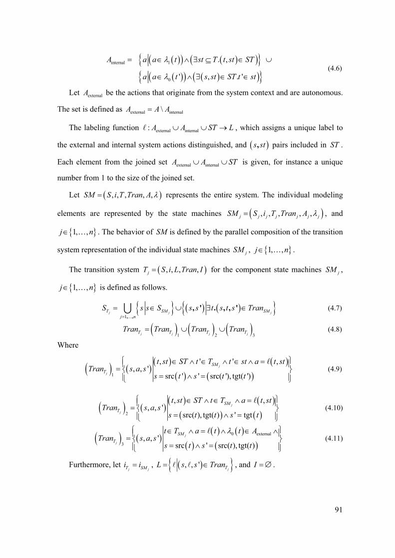
91
( )( ) ( )( ){ }( )( ) ( )( ){ }
internal 1
0
. ,
' , . '
A a a t st T t st ST
a a t s st ST t st
λ
λ
= ∈ ∧ ∃ ⊆ ∈ ∪
∈ ∧ ∃ ∈ ∈ (4.6)
Let externalA be the actions that originate from the system context and are autonomous.
The set is defined as external internal\A A A=
The labeling function external internal: A A ST L∪ ∪ → , which assigns a unique label to
the external and internal system actions distinguished, and ( ),s st pairs included in ST .
Each element from the joined set external internalA A ST∪ ∪ is given, for instance a unique
number from 1 to the size of the joined set.
Let ( ), , , , ,SM S i T Tran A λ= represents the entire system. The individual modeling
elements are represented by the state machines ( ), , , , ,j j j j j j jSM S i T Tran A λ= , and
{ }1, ,j n∈ … . The behavior of SM is defined by the parallel composition of the transition
system representation of the individual state machines jSM , { }1, ,j n∈ … .
The transition system ( ), , , ,jT S i L Tran I= for the component state machines jSM ,
{ }1, ,j n∈ … is defined as follows.
{ } ( ) ( ){ }1
j j jT SM SMj n
S s s S s s t s t s Tran=
= ∈ ∪ ∃ ∈, ,
, ' . , , '…∪ (4.7)
( ) ( ) ( )1 2 3j j j jT T T TTran Tran Tran Tran= ∪ ∪ (4.8)
Where
( ) ( )( ) ( )
( ) ( )1
, ' ' ,, , '
src ' ' src( '), tgt( ')j
j
SMT
t st ST t T t st a t stTran s a s
s t s t t
⎧ ⎫∈ ∧ ∈ ∧ ∈ ∧ =⎪ ⎪= ⎨ ⎬= ∧ =⎪ ⎪⎩ ⎭
(4.9)
( ) ( )( ) ( )
( ) ( )2
, ,, , '
src( ), tgt( ) ' tgtj
j
SMT
t st ST t T a t stTran s a s
s t t s t
⎧ ⎫∈ ∧ ∈ ∧ =⎪ ⎪= ⎨ ⎬= ∧ =⎪ ⎪⎩ ⎭
(4.10)
( ) ( )( ) ( )
( ) ( )0 external
3, , '
src ' src( ), tgt( )j
j
SMT
t T a t t ATran s a s
s t s t t
λ⎧ ⎫∈ ∧ = ∧ ∈ ∧⎪ ⎪= ⎨ ⎬= ∧ =⎪ ⎪⎩ ⎭
(4.11)
Furthermore, let j jT SMi i= , ( ){ }, , '
jTL s s Tran= ∈ , and I = ∅ .

92
Besides the states of jSM , new nodes are introduced in jTS . Transitions have an
input and an output set that becomes active one after the other. Two steps are discerned
in a transition. Each step is represented by a transition in T . The newly introduced state
represents the situation in which the first transition took place, but the second one needs
still to happen. Intermediate states are to be introduced for each transition
( )jSMs t s Tran∈, , ' .
The transitions in set ( )1jTTran correspond to the first step of the state machine
transition. The transitions in set ( )2jTTran correspond to the second step of the state
machine transition. The transitions in set ( )3jTTran correspond to the autonomous
actions that originate from the system’s context. The initial state of the transition system
corresponds to the state machine initial state. The set L denotes the system actions
distinguished. The state machine and transition system are both sequential; the
independence relation is an empty set.
4.3 Multi-Event Abstraction
Each state machine transition /a O
→ is modeled by two transitions in the transition
system model (and its elementary net system representation). One transition corresponds
to the input action a , and the other transition represents the occurrence of the system
actions in O . The distinction between local states and intermediate states is made, and
the states associated with the two transitions belong to these two different categories.
Let /
'a O
s s→ denote the state machine transition from s to 's . If O is not empty then
an additional state ( ), 's s is introduced. It denotes the intermediate state between s and
's , and describes the situation in which the conditional action a has been completed,
and the system actions in O are enabled but have not been fired. If O is empty then no
intermediate state is added and the state machine transition takes place between the local
states s and 's .
In order to adequately represent the SA/RT model execution rules, the notion of the
internal and external system actions is introduced. The time interval between the

93
consecutive internal system actions is relatively shorter than that between the
autonomous external system actions.
In case the external system actions are causally dependent, their execution is
separated in time. The occurrences of external system actions take place autonomously.
The external system actions that are independent of each other are considered as follows
in the behavioral model. The independent external system actions are possibly active at
the same time, or are separated in time and take place one after the other. The amount of
time is however undetermined and external system actions take place asynchronously.
The execution of internal system actions takes place in virtually zero time. Even if
consecutive internal system actions have causal dependency relationships, their
occurrences are at virtually the same point in time.
Whereas the external system actions are autonomous, the internal system actions are
invoked by either another internal system action or an external system action. For
example, the system actions that indicate the completion of the main task body are
autonomous, as are the system actions that originate from the system’s context. The
occurrence of the autonomous external system actions is not determined within the
system, but determined by the system’s context.
For the purposes of the behavioral analysis, it is sufficient to describe the system
behavior in terms of the external system actions as shown subsequently. The external
actions originate from the system’s context and are autonomous. An autonomous action
possibly causes some consequent transitions in the system, which take place in virtually
zero time and happen at the same time instant as the external action. The internal actions
resulting from an external system action and the associated states are grouped into so-
called multi-event transitions. A multi-event transition is a partial order of system
transitions that is initiated by an external action, and further includes all consequent
transitions that can take place in virtually zero time. Multi-event transitions group
elementary transitions into abstract transitions that hide the causal relations of the
underlying original transitions. Doing so, one can obtain a simpler, more abstract view of
the behavior. A group of elementary transitions can then be seen as a single entity; its
occurrence all depends on whether the corresponding external system action takes place.
The primary reason for the introduction of multi-event transitions is that the system
architecture is distributed. The behavior model however involves a mix of

94
communication and synchronization actions that either take place instantaneously in
virtual zero time, or asynchronously. Because the mapping of the system behaviour
(network of the system processes) on the system structure is yet to be defined, transitions
are constructed such that they all take place asynchronously and that they represent the
original synchronous and asynchronous ones. Rendezvous communication is used for
analysis. This way the formal basis is uniform for all possible sub-systems boundaries.
Conflict resolution is another reason for the introduction of multi-event transitions.
The external actions that are themselves not in conflict possibly have consequent
instantaneous transitions that are. In case non-conflicting external actions are fired
simultaneously, then possible conflict caused by subsequent instantaneous transients are
only detected after firing The conditions that precede such a group of transitions need to
be known first, in order to determine whether not only the external action and but also its
consequent transitions are non-conflicting. The multi-event transitions represent groups
of transitions that can be executed in virtually zero time, and have causal relationships.
The multi-event transitions render the conditions that precede such groups of transitions.
By grouping transitions into a smaller number of bigger entities, the analysis
(simulation) becomes more efficient. The internal causal relationships between
transitions of the multi-event transition can be hidden, since only the change caused by
the events is of interest for the behavioral analysis. The number of states and transitions
that need to be considered is in most cases substantially reduced by the introduction of
the multi-event transitions.
4.4 Behavioral Modeling of Multi-event transitions
4.4.1 Transition System Model
In transition systems as introduced in Chapter 2, all transitions are equal and the
notion of multi-events is unknown. The following behavior is attached to the notion of
multi-event transitions and modeled by transition systems that have extended execution
rules. Internal actions take place instantaneously, in virtual zero time. This implies that a
sequence of all synchronous actions cannot be broken up by the occurrence of an
external action, since the synchronous actions then logically wouldn’t take place in an
instant. Transition systems that represent SA/RT models do not include event sequences
where external actions occurrences are interleaved with synchronous events. Such a
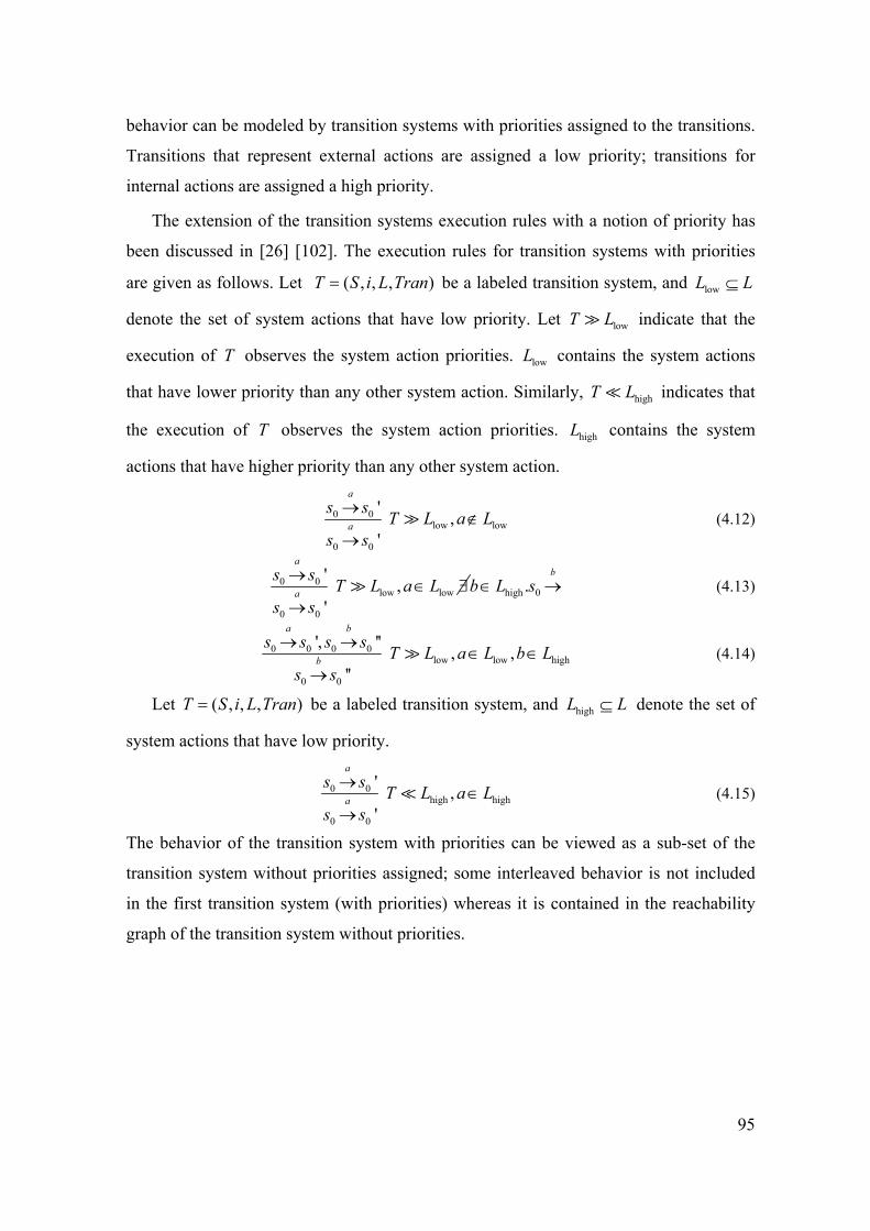
95
behavior can be modeled by transition systems with priorities assigned to the transitions.
Transitions that represent external actions are assigned a low priority; transitions for
internal actions are assigned a high priority.
The extension of the transition systems execution rules with a notion of priority has
been discussed in [26] [102]. The execution rules for transition systems with priorities
are given as follows. Let ( , , , )T S i L Tran= be a labeled transition system, and lowL L⊆
denote the set of system actions that have low priority. Let lowT L indicate that the
execution of T observes the system action priorities. lowL contains the system actions
that have lower priority than any other system action. Similarly, highT L indicates that
the execution of T observes the system action priorities. highL contains the system
actions that have higher priority than any other system action.
0 0low low
0 0
' ,'
a
a
s s T L a Ls s
→∉
→ (4.12)
0 0low low
0 0
' ,'
a
a
s s T L a Ls s
→∈ ∃
→high 0.
bb L s∈ → (4.13)
0 0 0 0low low high
0 0
', '' , ,''
a b
b
s s s s T L a L b Ls s
→ →∈ ∈
→ (4.14)
Let ( , , , )T S i L Tran= be a labeled transition system, and highL L⊆ denote the set of
system actions that have low priority.
0 0high high
0 0
' ,'
a
a
s s T L a Ls s
→∈
→ (4.15)
The behavior of the transition system with priorities can be viewed as a sub-set of the
transition system without priorities assigned; some interleaved behavior is not included
in the first transition system (with priorities) whereas it is contained in the reachability
graph of the transition system without priorities.

96
97
Chapter 5.
Internal Model
5.1 Introduction
A number of different model types are used to attach an approximate behavior to
SA/RT models in the research reported in this thesis. Each of them serves a certain
specific purpose. Whereas SA/RT models themselves are well suited for the initial
specification, they miss a formal base for behavioral analysis. The primitive processes
and connectors of the SA/RT model are for this reason first modeled as individual
(sequential) state machines, which in turn are translated into transition systems. As
discussed in Chapter 2, the joint behavior attached to the SA/RT model is given by the
composite transition system for the primitive processes and connectors. The construction
of a composite transition system from primitive ones is however difficult; it is however
far less complicated to first translate the individual transition systems into elementary net
systems, and perform the composition on them. Whereas the transition systems provide
the structuring concepts for modeling the behavioral aspects of a real-time embedded
system, they do not offer a structure that is directly suited for implementation of the
composition operator and behavioral analysis. Elementary net systems offer such a
structure. Elementary net systems on their turn lack concepts for structuring the system
behavior. In the research reported in this thesis, elementary net systems are used to
represent the transition systems. The composite elementary net system then represents
the composite transition system, and renders the behavior attached to the SA/RT model.
A composition operator for elementary net systems is defined that comply with the
composition operator for transition systems. In contrast to the composition operator for
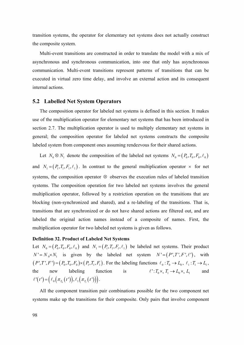
98
transition systems, the operator for elementary net systems does not actually construct
the composite system.
Multi-event transitions are constructed in order to translate the model with a mix of
asynchronous and synchronous communication, into one that only has asynchronous
communication. Multi-event transitions represent patterns of transitions that can be
executed in virtual zero time delay, and involve an external action and its consequent
internal actions.
5.2 Labelled Net System Operators
The composition operator for labeled net systems is defined in this section. It makes
use of the multiplication operator for elementary net systems that has been introduced in
section 2.7. The multiplication operator is used to multiply elementary net systems in
general; the composition operator for labeled net systems constructs the composite
labeled system from component ones assuming rendezvous for their shared actions.
Let 0 1N N⊗ denote the composition of the labeled net systems ( )0 0 0 0 0, , ,N P T F=
and ( )1 1 1 1 1, , ,N P T F= . In contrast to the general multiplication operator × for net
systems, the composition operator ⊗ observes the execution rules of labeled transition
systems. The composition operation for two labeled net systems involves the general
multiplication operator, followed by a restriction operation on the transitions that are
blocking (non-synchronized and shared), and a re-labeling of the transitions. That is,
transitions that are synchronized or do not have shared actions are filtered out, and are
labeled the original action names instead of a composite of names. First, the
multiplication operator for two labeled net systems is given as follows.
Definition 32. Product of Labeled Net Systems Let ( )0 0 0 0 0, , ,N P T F= and ( )1 1 1 1 1, , ,N P T F= be labeled net systems. Their product
0 1'N N N= × is given by the labeled net system ( )' ', ', ', 'N P T F= , with
( ) ( ) ( )0 0 0 1 1 1', ', ' , , , ,P T F P T F P T F= × . For the labeling functions 0 0 0:T L→ , 1 1 1:T L→ ,
the new labeling function is 0 1 0 1' :T T L L∗ ∗× → × and
( ) ( )( ) ( )( )( )0 10 1' ' ' , 'T Tt t tπ π= .
All the component transition pair combinations possible for the two component net
systems make up the transitions for their composite. Only pairs that involve component
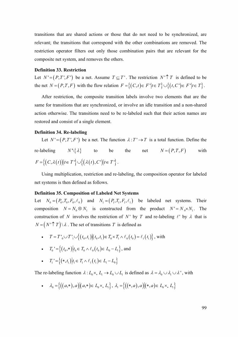
99
transitions that are shared actions or those that do not need to be synchronized, are
relevant; the transitions that correspond with the other combinations are removed. The
restriction operator filters out only those combination pairs that are relevant for the
composite net system, and removes the others.
Definition 33. Restriction Let ( )' , ', 'N P T F= be a net. Assume 'T T⊆ . The restriction 'N T↑ is defined to be
the net ( ), ,N P T F= with the flow relation ( ){ } ( ){ }, ' , ' 'F C t F t T t C F t T= ∈ ∈ ∪ ∈ ∈ .
After restriction, the composite transition labels involve two elements that are the
same for transitions that are synchronized, or involve an idle transition and a non-shared
action otherwise. The transitions need to be re-labeled such that their action names are
restored and consist of a single element.
Definition 34. Re-labeling Let ( )' , ', 'N P T F= be a net. The function : 'T Tλ → is a total function. Define the
re-labeling { }'\N λ to be the net ( ), ,N P T F= with
( )( ){ } ( )( ){ }, ' , ' 'F C t t T t C t Tλ λ= ∈ ∪ ∈ .
Using multiplication, restriction and re-labeling, the composition operator for labeled
net systems is then defined as follows.
Definition 35. Composition of Labeled Net Systems Let ( )0 0 0 0 0, , ,N P T F= and ( )1 1 1 1 1, , ,N P T F= be labeled net systems. Their
composition 0 1N N N= ⊗ is constructed from the product 0 1'N N N= × . The
construction of N involves the restriction of 'N by T and re-labeling ' by λ that is
( )' \N N T λ= ↑ . The set of transitions T is defined as
• ( ) ( ) ( ) ( ){ }0 1 0 1 0 1 0 1 0 0 1 1' ' , ,T T T t t t t T T t t= ∪ ∪ ∈ × ∧ = , with
• ( ) ( ){ }0 0 0 0 0 0 0 1' ,T t t T t L L= ∗ ∈ ∧ ∈ − , and
• ( ) ( ){ }1 1 1 1 1 1 1 0' ,T t t T t L L= ∗ ∈ ∧ ∈ −
The re-labeling function 0 1 0 1: L L L Lλ ∗× → ∪ is defined as 0 1 'λ λ λ λ= ∪ ∪ , with
• ( )( ) ( ){ }0 0 1, , ,a a a L Lλ ∗= ∗ ∗ ∈ × , ( )( ) ( ){ }1 0 1, , ,a a a L Lλ ∗= ∗ ∗ ∈ ×

100
• ( )( ) ( ){ }0 1' , , ,a a a a a L Lλ ∗= ∈ ×
Constructing the composition of the underlying labeled net systems, and specifying
the composite system’s initial state result in the composition of two labeled elementary
net systems.
Definition 36. Composition of Labeled Elementary Net Systems Let ( ), , , , inN P T F C= , and 0 1N N N= ⊗ be the composed elementary of
( )( )0 0 0 0 0 0, , , , inN P T F C= and ( )( )1 1 1 1 1 1
, , , , inN P T F C= . The construction of N is
defined as follows.
• ( ) ( ) ( )0 0 0 0 1 1 1 1, , , , , , , , ,P T F P T F P T F= ⊗
• ( )( ) ( )( )0 1 10in in inC C Cµ µ= ∪
5.3 Behavioral Modeling of Multi-Event Transitions
In order to attach behavior, in terms of transition systems that includes multi-events
to SA/RT models, transitions are given priorities. The transition is assigned a high or low
priority depending on whether they are internal or external actions respectively. A notion
of priorities needs also to be introduced for elementary net systems that represent these
transition systems.
The notion of concession has been discussed in section 2.5; here the transitions are
not assigned any priorities and are all equal. The conditions for the firing of transitions
that have priorities (two level) are given by the concessions: highcon and lowcon. The
relation t Chighcon expresses that transition t has high priority and has concession at
C ; it is defined as follows.
Definition 37. High Priority Concession Let N be a net system with markings C , 'C and transition t . The set 'T T⊆ contains
transitions, which are assigned a high priority. If 't T∈ then 't
C C→ if and only if
Ct con .
The relation t Clowcon expresses that transition t has low priority and has concession
at C ; it is defined as follows.
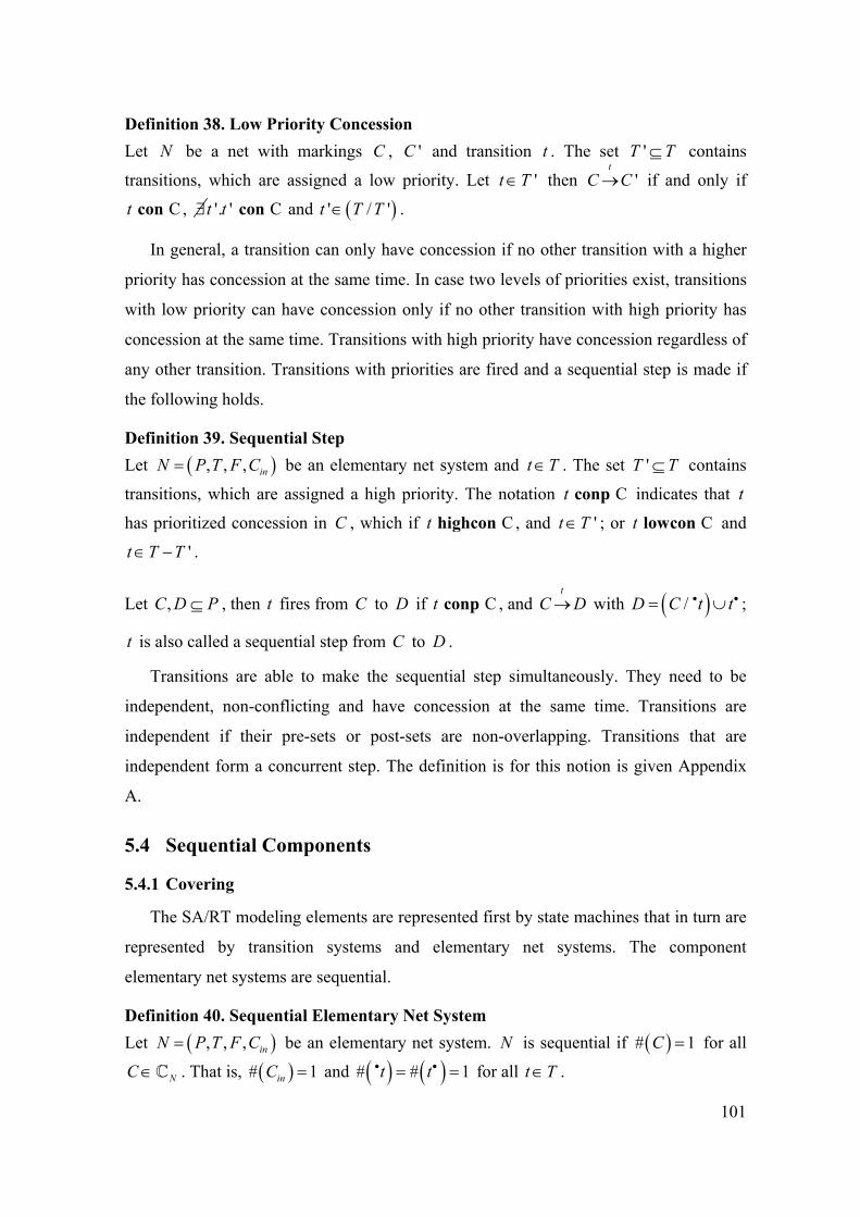
101
Definition 38. Low Priority Concession Let N be a net with markings C , 'C and transition t . The set 'T T⊆ contains
transitions, which are assigned a low priority. Let 't T∈ then 't
C C→ if and only if
Ct con , ∃ '. ' Ct t con and ( )' / 't T T∈ .
In general, a transition can only have concession if no other transition with a higher
priority has concession at the same time. In case two levels of priorities exist, transitions
with low priority can have concession only if no other transition with high priority has
concession at the same time. Transitions with high priority have concession regardless of
any other transition. Transitions with priorities are fired and a sequential step is made if
the following holds.
Definition 39. Sequential Step Let ( ), , , inN P T F C= be an elementary net system and t T∈ . The set 'T T⊆ contains
transitions, which are assigned a high priority. The notation Ct conp indicates that t
has prioritized concession in C , which if Ct highcon , and 't T∈ ; or Ct lowcon and
't T T∈ − .
Let ,C D P⊆ , then t fires from C to D if Ct conp , and t
C D→ with ( )/D C t t• •= ∪ ;
t is also called a sequential step from C to D .
Transitions are able to make the sequential step simultaneously. They need to be
independent, non-conflicting and have concession at the same time. Transitions are
independent if their pre-sets or post-sets are non-overlapping. Transitions that are
independent form a concurrent step. The definition is for this notion is given Appendix
A.
5.4 Sequential Components
5.4.1 Covering
The SA/RT modeling elements are represented first by state machines that in turn are
represented by transition systems and elementary net systems. The component
elementary net systems are sequential.
Definition 40. Sequential Elementary Net System Let ( ), , , inN P T F C= be an elementary net system. N is sequential if ( )# 1C = for all
NC ∈C . That is, ( )# 1inC = and ( ) ( )# # 1t t• •= = for all t T∈ .

102
Let 0 1N N N= ⊗ , and 0N is a labeled net system that underlies a sequential labeled
elementary net systems. Furthermore let 1N be the results of a composition of labeled net
systems that each underlie a sequential labeled elementary net system. The net system N
underlies the composition of a number of sequential labeled elementary net systems.
The following relations holds between a composite elementary net system and its
component net systems. The behavior of N is related to the behavior of 0N and 1N by
't
C C→ in 0 1N N⊗ if and only if ( )( )
( )0
0 0 't
C Cµ
π π→ , and ( )( )
( )1
1 1
t
t tµ
π π→ .
• If ( ) ( ){ }0 0 0 0 0 0 0 1' ,t T t t T t L L∈ = ∗ ∈ ∧ ∈ − then there is transition 0
't
c c→ in 0N ,
such that c C∈ , ' 'c C∈ , { } ' { '}C c C c− = − , ( )0 C cπ = , ( )0 ' 'C cπ = , and
( )0 0t tµ = .
• If ( ) ( ){ }1 1 1 1 1 1 1 0' ,t T t t T t L L∈ = ∗ ∈ ∧ ∈ − then there is transition 1
't
D D→ , such
that D C⊂ , ' 'D C⊂ , ' 'C D C D− = − , ( )1 C Dπ = , ( )1 ' 'C Dπ = , and ( )1 1t tµ = .
• If ( ) ( ) ( ) ( ){ }0 1 0 1 0 1 0 0 1 1, ,t t t t t T T t t∈ ∈ × ∧ = then there are transitions 0
't
c c→ in
0N , and 1
't
D D→ in 1N , and both condition lists listed above hold.
Let ( )0 0 0 0 0' ', ', ', 'N P T F= , 0 0'P P= be a sub-system that is constructed according to the
definition below. The labeled net system 0 'N is a sequential component of N .
Definition 41. Sub-system Let ( ), , , inN P T F C= be an elementary net system and let 'P P⊆ . Let
( )' ', ', ', 'inN P T F C= be the subsystem of N determined by 'P . 'N is constructed as
follows: ( )' 'T P= nbh , ( ) ( )( )' ' ' ' 'F F P T T P= ∩ × ∪ × and ' 'in inC C P= ∩ .
Definition 42. Sequential Component Let ( ), , , inN P T F C= be an elementary net system and let 'P P⊆ . Let
( )' ', ', ', 'inN P T F C= be the subsystem of N determined by 'P . If ( )# ' 1C P∩ = for all
NC ∈C then 'N is a sequential component of N .

103
Let 0 1 mP P P P= … denote the set of places of N , and 0 1, , , mP P P… are the set
of places for the component labeled elementary net systems. Let 0 1, , , mP P P… define the
sub-systems 0 1', ', , 'mN N N… of N using the definition above (Definition 41). The sub-
systems are sequential components of N , and cover N .
Definition 43. Covering Let ( ), , , inN P T F C= be an elementary net system. A set { }1, , mN N… of subsystems of
N , with ( )( ), , ,i i i i in iN P T F C= , 1 i m≤ ≤ , 0m ≥ , is a covering of N if 1
mii
P P=
=∪ ,
1
mii
T T=
=∪ , 1
mii
F F=
=∪ , and ( )1
min in ii
C C=
=∪ . N is covered by sequential components, if
iN is a sequential component of N for every 1 i m≤ ≤ .
5.4.2 Contact-Freeness
A transition can only be fired if it has input-concession and output-concession. A
contact-free transition never has input-concession and output-concession simultaneously.
For contact-free transitions, it is sufficient to only determine whether a transition has
input-concession, in order to determine whether it can be fired. An elementary net
system is contact free if all its transitions are contact-free. Generally, in order to
determine whether an elementary net system is contact-free requires the computation of
all reachable configurations. This is computationally expensive. Elementary net systems
that can be covered by sequential components are however contact-free [126].
Generating the net system representation for SA/RT models results in a system that
has a covering by sequential components. Concession within the elementary net system
only involves checking the pre-sets.
5.4.3 Characterization of States and Actions
The SA/RT modeling element such as transformations, branches and merges can be
assigned a unique number. That is, each sequential component is assigned a unique
number.
The elements ( )X P T= ∪ of the composed net system are each associated with a
one ore more sequential components. Let ( ): Xη → P be the function that assigns a
set of sequential component numbers to each element ( )x P T∈ ∪ . The numbers in the
set indicate the sequential components to which the elements are attached.
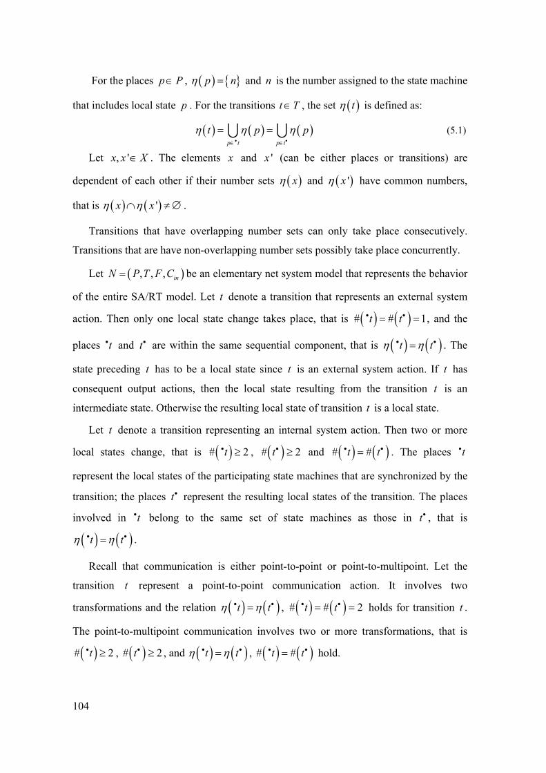
104
For the places p P∈ , ( ) { }p nη = and n is the number assigned to the state machine
that includes local state p . For the transitions t T∈ , the set ( )tη is defined as:
( ) ( ) ( )p t p t
t p pη η η• •∈ ∈
= =∪ ∪ (5.1)
Let , 'x x X∈ . The elements x and 'x (can be either places or transitions) are
dependent of each other if their number sets ( )xη and ( )'xη have common numbers,
that is ( ) ( )'x xη η∩ ≠ ∅ .
Transitions that have overlapping number sets can only take place consecutively.
Transitions that are have non-overlapping number sets possibly take place concurrently.
Let ( ), , , inN P T F C= be an elementary net system model that represents the behavior
of the entire SA/RT model. Let t denote a transition that represents an external system
action. Then only one local state change takes place, that is ( ) ( )# # 1t t• •= = , and the
places t• and t• are within the same sequential component, that is ( ) ( )t tη η• •= . The
state preceding t has to be a local state since t is an external system action. If t has
consequent output actions, then the local state resulting from the transition t is an
intermediate state. Otherwise the resulting local state of transition t is a local state.
Let t denote a transition representing an internal system action. Then two or more
local states change, that is ( )# 2t• ≥ , ( )# 2t• ≥ and ( ) ( )# #t t• •= . The places t•
represent the local states of the participating state machines that are synchronized by the
transition; the places t• represent the resulting local states of the transition. The places
involved in t• belong to the same set of state machines as those in t• , that is
( ) ( )t tη η• •= .
Recall that communication is either point-to-point or point-to-multipoint. Let the
transition t represent a point-to-point communication action. It involves two
transformations and the relation ( ) ( )t tη η• •= , ( ) ( )# # 2t t• •= = holds for transition t .
The point-to-multipoint communication involves two or more transformations, that is
( )# 2t• ≥ , ( )# 2t• ≥ , and ( ) ( )t tη η• •= , ( ) ( )# #t t• •= hold.
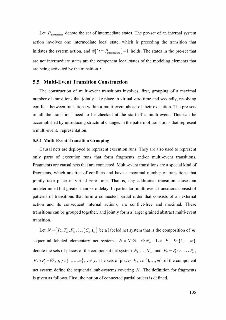
105
Let intermediateP denote the set of intermediate states. The pre-set of an internal system
action involves one intermediate local state, which is preceding the transition that
initiates the system action, and ( )intermediate# 1t P• ∩ = holds. The states in the pre-set that
are not intermediate states are the component local states of the modeling elements that
are being activated by the transition t .
5.5 Multi-Event Transition Construction
The construction of multi-event transitions involves, first, grouping of a maximal
number of transitions that jointly take place in virtual zero time and secondly, resolving
conflicts between transitions within a multi-event ahead of their execution. The pre-sets
of all the transitions need to be checked at the start of a multi-event. This can be
accomplished by introducing structural changes in the pattern of transitions that represent
a multi-event. representation.
5.5.1 Multi-Event Transition Grouping
Causal nets are deployed to represent execution runs. They are also used to represent
only parts of execution runs that form fragments and/or multi-event transitions.
Fragments are causal nets that are connected. Multi-event transitions are a special kind of
fragments, which are free of conflicts and have a maximal number of transitions that
jointly take place in virtual zero time. That is, any additional transition causes an
undetermined but greater than zero delay. In particular, multi-event transitions consist of
patterns of transitions that form a connected partial order that consists of an external
action and its consequent internal actions, are conflict-free and maximal. These
transitions can be grouped together, and jointly form a larger grained abstract multi-event
transition.
Let ( )( ), , , ,N N N N in NN P T F C= be a labeled net system that is the composition of m
sequential labeled elementary net systems 1 mN N N= ⊗ ⊗… . Let iP , { }1, ,i m∈ …
denote the sets of places of the component net system 1, , mN N… , and 1N mP P P= ∪ ∪… ,
i jP P∩ = ∅ , { }, 1, ,i j m∈ … , i j≠ . The sets of places iP , { }1, ,i m∈ … of the component
net system define the sequential sub-systems covering N . The definition for fragments
is given as follows. First, the notion of connected partial orders is defined.

106
Definition 44. Connected Partial Order Let ( ),X ρ be a partial ordered set. It is connected if for each pair of elements , 'x x X∈ ,
'x x≠ , the property ( ) ( )1, 'x x ρ ρ+−∈ ∪ holds. Here ( ) ( ){ }1 , ' ',x x x xρ ρ− = ∈ is the
inverse of partial order ρ .
Definition 45. Fragments Let ( )1 2, , , ,M M MM P T F φ φ= be a labeled causal net. It is a fragment of N if
• ( ), ' M Mx x X X∈ × are connected.
• Mt T∈ , ( ) ( )( )1 2t tφ φ•• = , ( ) ( )( )1 2t tφ φ
•• =
• 1φ is an injection for each cut of the partial order ( ),X F +
• If ( )1 ip Pφ ∈ then there is a line L , such that ( )1 M iL P Pφ ∩ ⊆ , and
( )1 M iP L Pφ − ∩ = ∅
• Mp P∈ , ( ) ( )( )2 1p pφ φ•• = , ( ) ( )( )2 1p pφ φ
•• = , ( ) ( )# # 1p p= =i i
Definition 46. Conflict-free Fragments A fragment is conflict-free if for all Mt T∈ , t M• ⊆/ ,
( ) ( )1 2' , ' 'Nt T t t t tφ φ• •∈ ∩ ≠ ∅ ⇒ = .
Transitions in a conflict-free fragment, except the first one, have pre-sets that are non-
conflicting.
Definition 47. Prioritized Fragment A fragment is prioritized if for Mt T∈ , t M• ⊆/ , ( )2 tφ has high priority, and there is one
' Nt T∈ , ( )1't Mφ• ⊆ and 't has low priority.
A prioritized fragment sets out with a low priority transition, followed by only transitions
with high priority.
Definition 48. Maximal prioritized fragments A prioritized fragment is maximal if for Nt T∈ , ( )1 M tφ •∩ ≠ ∅ then t has low priority;
( )1 Mφ are all local states.

107
The final part of maximal prioritized fragments consists of all local states; no transition
can be appended to a maximal prioritized fragment anymore.
Maximal, prioritized and conflict-free fragments form multi-event transitions. They
are constructed by grouping an external system action and its consequent internal system
actions together.
Let ( )1 2, , , ,M M MM P T F φ φ= be a prioritized fragment, ( ), , , inN P T F C= is the
corresponding elementary net system, and ( )( ), , ,i i i i in iN P T F C= , 1 i m≤ ≤ , are
sequential components covering N . Let Nu T∈ be a transition with which M is
extended to 'M . 'M is in turn a prioritized fragment if
• u is a high priority transition
• 'M MP P⊂ , 'M MT T⊂ , 'M MF F⊂
• { }'M MT T s= ∪ and ( )s uφ =
• the resulting partial order is connected: ( )M uφ •∩ ≠ ∅
• p M∈ , 'p s•∈ , ( ) ( )' 'p p p pφ φ= ⇒ = and there is a line L , with
( )M iL P Pφ ∩ ⊆ , and ( )M iP L Pφ − ∩ = ∅ such that ( ) ( )' ip p Pφ φ= ∈ , i.e. in
case the places in the pre-set of u are the same as the places M represent then
they are represented by a the same place in the fragment.
• 'p s•∈ , ( ) ( )'p Mφ φ∉ , ' Mp P∉ , '' Mp P∈ and there is no line L , with
( )M iL P Pφ ∩ ⊆ , and ( )M iP L Pφ − ∩ = ∅ such that ( ) ( )' ip p Pφ φ= ∈ , i.e. in
case the places in the pre-set of u are the same as the places M represent then a
new place is introduced in 'M ; the place is not part of a sequential component
already present in the fragment
• Ms P• ∩ = ∅ , 'Ms P• ⊂ i.e. places for the post-set of s are newly introduced in
'M
• ( )s uφ = , p s•∀ ∈ . ( ) ', Mp s F∈ and p s•∀ ∈ . ( ) ', Ms p F∈ the flow relation 'MF is
an extension of MF with the causal relation of u .
108
The initial and final parts of a multi-event transition involves local states only; the
partial order cuts involve both local and intermediates states. The component transitions
in a multi-event transition are all internal actions, except the action initiating the multi-
event transition, which is an external (and autonomous) action.
5.5.2 Resolving Conflicts between Multi-Event Transitions
Multi-event transitions are non-conflicting if the individual transitions that make up
the multi-event transitions are non-conflicting. Transitions in two different multi-event
transitions then need to have non-overlapping pre-sets, in order for the multi-events they
belong to, to be non-conflicting. It is for this reason not sufficient to only consider the
pre-sets of the transitions with which multi-events set out. Let t and 't be transitions that
correspond to the external autonomous system actions that have non-overlapping pre-
sets. They may be fired simultaneously, causing their consequent actions to take place
within the same instant. Although the pre-sets of t and 't are non-overlapping, the pre-
sets of their consequent transitions are possibly overlapping. The situation occurs in
which conflicts are detected only at the start of the consequent transitions that are
conflicting, which is after the multi-event transitions have set out. In order to resolve this
kind of conflicts, only one of the initiating actions should have been fired; the pre-sets of
the consequent transitions should already be checked at the point at which the multi-
event transitions set out.
The grouping of transitions in order to identify multi-events, renders patterns of
transitions that are partial orders without branches. This means that its initial part and
final part determine the system state change, and cuts of M and 'M are non-
overlapping except those included in the initial and final parts. For multi-events, initial
parts that overlap are then the only cause for conflicts.
Let M and ( )'M denote the initial parts of M and 'M , then they are in conflict at
C if ( )1 M Cφ ⊆ , ( )( )1 'M Cφ ⊆ and ( ) ( )( )1 1 'M Mφ φ∩ ≠ ∅ .
Within elementary net systems, conflicts are resolved locally. Hereby, conditions of
the pre-sets belonging to other or future events are not being considered. Because all
events within a multi-event transition are causally dependent of the event that
corresponds with the initiating external system action and the initial part conditions are
109
the only cause for conflicts, multi-event transitions can complete their execution without
conflicts only if their initial parts non-overlapping when firing the external system
action.
In order to consider the initial part conditions at the time the external system action is
fired, certain modifications to the underlying multi-event net system representation are
introduced. The pre-set of the initiating external system action are extended with the
initial part conditions of the consequent transitions.
Let ( ) ( )( )1 2, , , ,M M M M MM P T F φ φ= be the labeled causal net that represents a
fragment of the elementary net system ( ), , ,N N N inN P T F C= and ( ),M M MP T F +∪ be the
partially ordered set defined by M . The modified multi-event
( ) ( )( )' ' ' 1 ' 2 '' , , , ,M M M M M
M P T F φ φ= is derived from M .
Let 0s be the event that is associated with the initiating external system action. Let
p be a condition that is included by the initial part of multi-event M , i.e. p M∈ .
Distinguished are two situations.
If p M∈ and ( )0,p s F∈ then p makes part of the pre-set of 0s and no
modification needs to be introduced. If p M∈ and ( )0,p s F∉ , then ( ), 'p s F∃ ∈ and
0's s≠ , the following modifications are introduced for each such ( ), 'p s . Let
( )' ', ', 'M B E F= denote the structurally changed elementary net system. 'N is
constructed as follows.
• 'M MP P= ,
• 'M MT T= ,
• ( ) ( ){ } ( ){ }0' \ , ' , , ' ,M M MF F p s p M p s F p s p M= ∈ ∈ ∪ ∈ .

110
5.6 Some Characteristics of the Composite Net System
5.6.1 Redundant Transitions
Firing sequences are sequences of sequential steps.. The set of all firing sequences of
N is denoted by ( )FS N . The set of all reachable configurations (states visited by
( )FS N ) of N is denoted by NC ; the computational costs for NC are usually very high.
The composite elementary net systems are constructed from the component net
systems. A transition is useful, if the state from which it emerges is reached. During the
composition, transitions are introduced that will possibly not be useful. In order to
determine the usefulness of transitions, the set of all reachable configurations NC needs
to be computed. NC is the set of all reachable configurations (states visited by ( )FS N
which is the set of all firing sequences of N ) and is expensive to compute. For this
reason, the computation of ( )FS N is withheld; transitions that are not useful in the
composite net system remain undetected.
5.7 Example
Figure 19 shows an example of a SA/RT model. It consists of four data
transformations, and a merge and a branch connector. For the mapping and scheduling
problem, a number of execution runs are taken into consideration. The causal relations
between the transformations in these runs need to be resolved. The transformation tr1,
exhibits the approximate behavior as shown in Figure 20. The transformation has two
execution modes. Depending on the mode executed, the transformation completes its run
with system action rdy1a or rdy1b. These two system actions result in different
consequent actions. The system action rdy1a will invoke transformation tr2; rdy1b will
invoke the transformations tr3 and tr4. In Figure 20 the state machine for the
approximate behavior of transformation tr2 is also given. The transformations tr2, tr3,
tr4 only have one execution mode.
The state machines representation for the SA/RT model is given in Figure 21. The
conditions and actions associated with the transitions are not shown in the figure in order
to avoid cluttering. For example, the transition numbered 0 is defined as /x
→ ; transitions
1 and 2 are defined as 1 /rdy a a
→ and 1 /rdy b b
→ respectively. For the same reason of avoiding
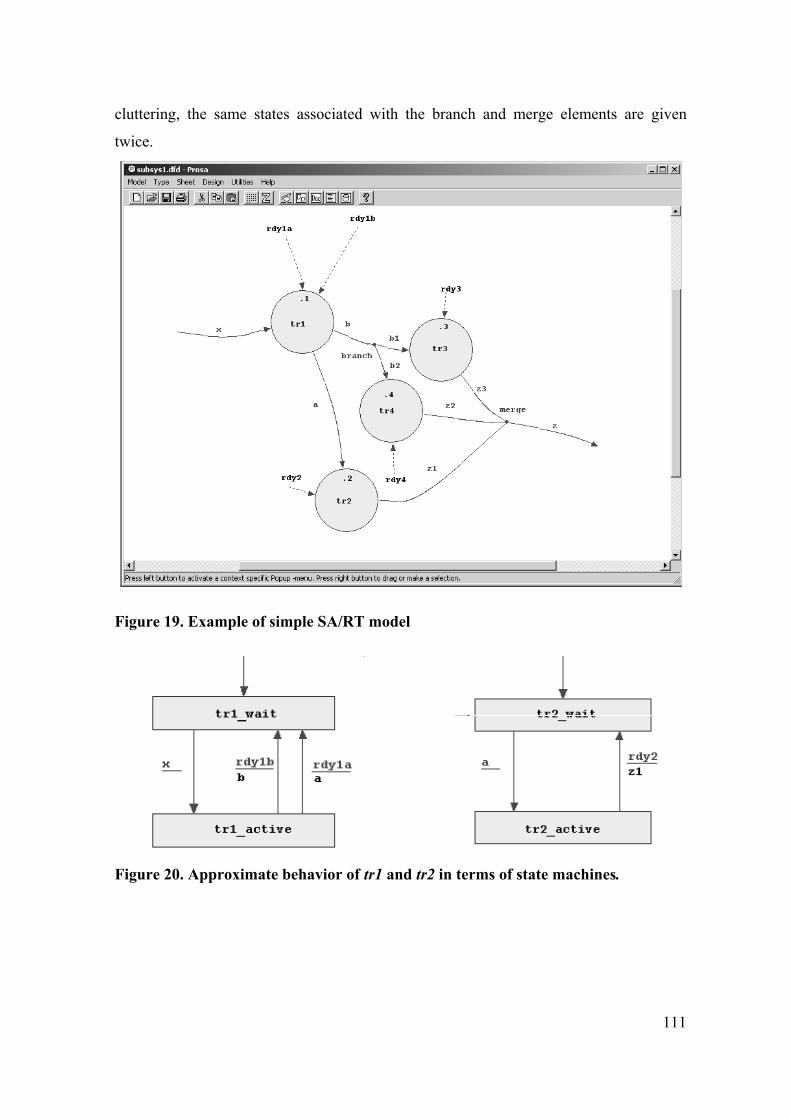
111
cluttering, the same states associated with the branch and merge elements are given
twice.
Figure 19. Example of simple SA/RT model
Figure 20. Approximate behavior of tr1 and tr2 in terms of state machines.
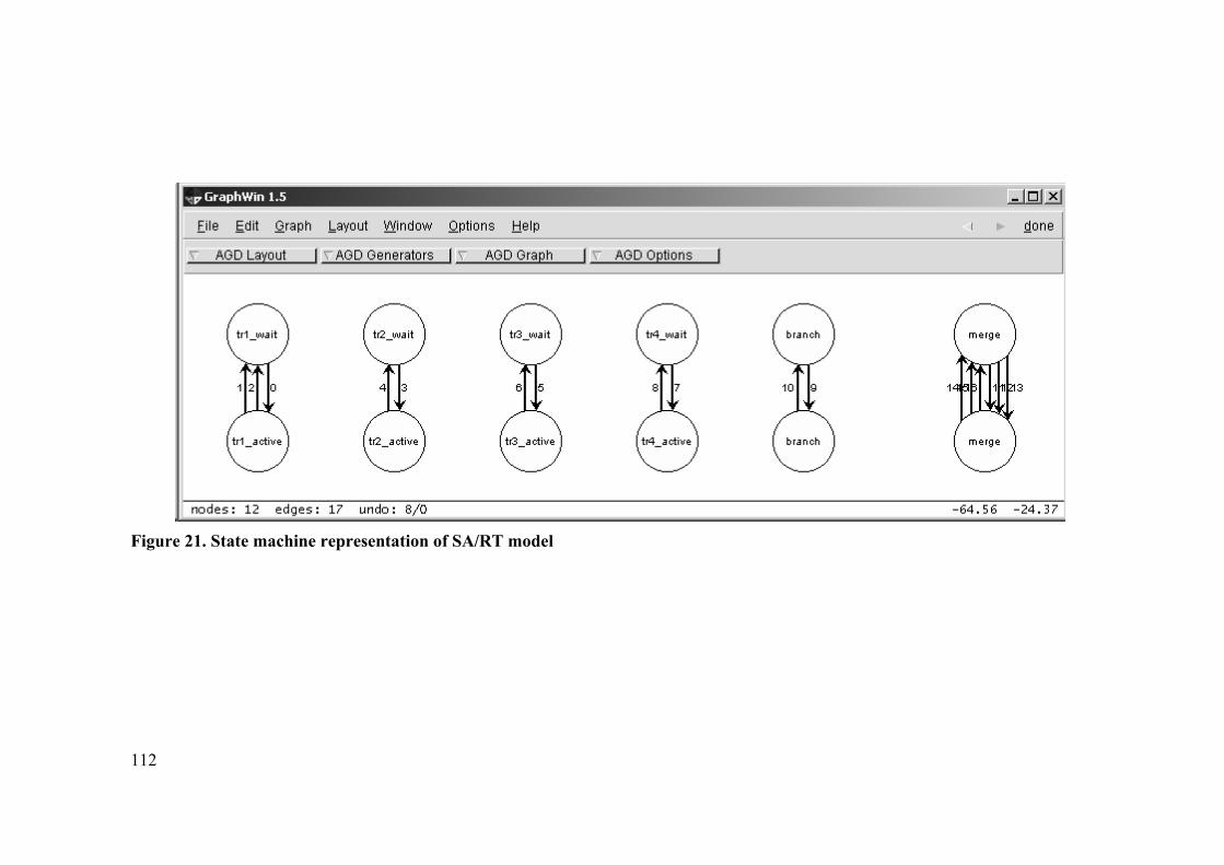
112
Figure 21. State machine representation of SA/RT model
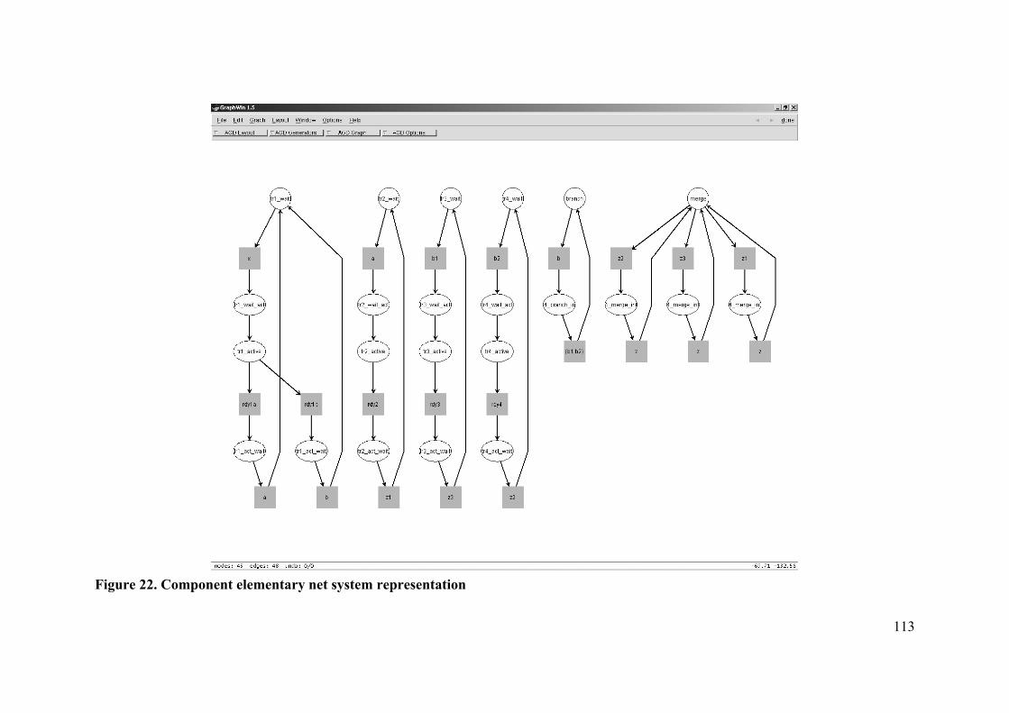
113
Figure 22. Component elementary net system representation

114
Figure 22 shows the component elementary net systems representation of the SA/RT
model. Each of the component elementary net systems represents a modeling element
from the SA/RT model. The elementary net systems are sequential and can be derived in
a straightforward manner from the state machines. The circles represent the system
actions; the rectangles are the conditions or places.
The composite elementary net system is obtained by component-wise applying the
composition operator. Figure 23 shows the end result of the composition. The places
colored in white are local conditions; the other places in gray are intermediate places.
The system actions colored in gray are external actions and have low priority; the
internal actions in white are internal actions and are assigned high priority.
The execution rules for elementary net systems with priorities have been discussed in
Chapter 5. An external action and its consequent actions form fragments, and are
executed in virtual zero time. Fragments and its notions have been introduced in Chapter
5. Figure 24 and Figure 25 shows two (out of six) fragments that can be formed for the
composite elementary net system of Figure 23.
The fragments can be collapsed to form an abstract multi-event transition. Figure 26
shows an elementary net system where the transitions are multi-event transitions.
Elementary net systems can be unfolded in order to provide an execution trace.
Figure 27 gives the causal relations between the system actions for the execution
sequence x, rdy1a, x, rdy1b, rdy2, rdy3, rdy4.
The reachability graph is given in Figure 28. Usually such a graph cannot be
computed due to the computational costs involved. The causal relations are resolved by
unfolding the composite elementary net system for a number of execution sequences.
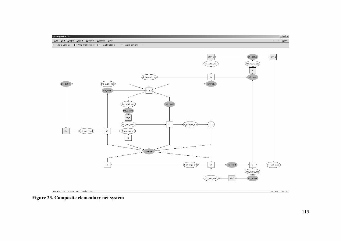
115
Figure 23. Composite elementary net system
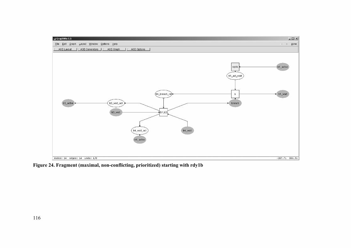
116
Figure 24. Fragment (maximal, non-conflicting, prioritized) starting with rdy1b

117
Figure 25. Fragment (maximal, non-conflicting, prioritized) starting with rdy3

118
Figure 26. Composite elementary net systems with fragments collapsed
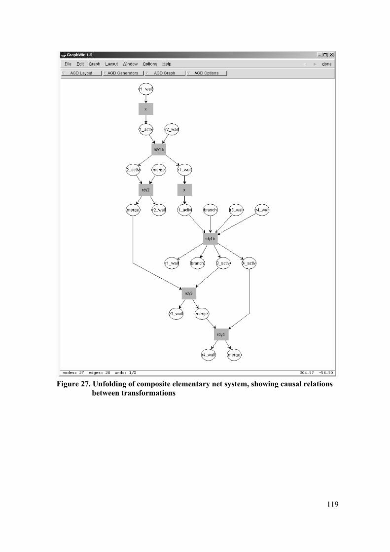
119
Figure 27. Unfolding of composite elementary net system, showing causal relations
between transformations
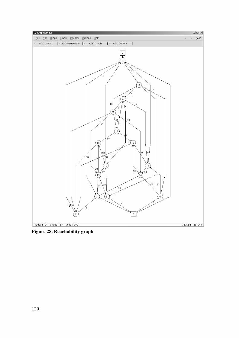
120
Figure 28. Reachability graph

121

123
Chapter 6.
Optimization Model
6.1 Introduction
Transformation runs and data transfers require the use of target architecture resources. In
order to use the resources as efficient as possible, (near-) optimal design decisions need
to be made that determines which transformation runs and data transfers should use
which resources, at what time and what duration.
In general such a problem can be formulated as a certain sort of multi-objective
decision making problem, and involve constraints, objectives, their aggregation structure,
and trade-off information. In this particular case, the choice was made to first specify the
decision space of the problem as a linear system, which in a satisfactory way resembles
the structure of the actual mapping and scheduling problem. A genetic representation of
the decision space is then developed based on the linear system specification, and the
search for a satisfying solution is implemented using genetic algorithms.
In the linear programming formulation the mapping and scheduling problem can be
structured as a function of some decision variables, in the presence of constraints. The
problem can be formulated as follows:
( )( )( )
1, ,1, ,
i i
j j
Minimize f xsubject to g x b i m
h x c j n≥ == =
……
(5.2)
Here x is a vector of decision variables, and ( )f ⋅ , ( )ig ⋅ and ( )jh ⋅ are linear
functions for decision variables. In the case the decision variables are discrete, an integer
linear programming problem is obtained. For linear programming problems (LP) some

124
efficient solution methods exist. ILP is however much more hard to solve, and usually
can only be solved heuristically.
Although ILP is in general not a successful route for finding solutions to
combinatorial problems, it can be helpful in defining more precisely the nature of a given
problem and finding its decision model. In this thesis, the ILP is used to formulate the
decision space of the mapping and scheduling problem. This is of particular importance
since a combination of genetic algorithm methods and constraints satisfaction techniques
is used to obtain some satisfactory solutions heuristically. The use of a linear system
representation ensures that the problem can be represented in both frameworks.
In the context of modeling the problem as a linear system, some generic modeling
constructs for certain problem classes exist. Their formulations can be used as a starting
point for formulating the particular problem representation for the genetic algorithm and
constraints satisfaction problem. In particular, the modeling constructs for assignment,
scheduling, and logical conditions such as implication and equivalence are used in this
thesis.
6.2 Behavioral Model
6.2.1 Task Graphs
In order to model the mapping and scheduling problem, a number of system runs or
use cases are selected to represent typical system behavior. The execution runs possible
for a system embodies its functionality. These use cases render building blocks for the
optimization model of the mapping and scheduling problem. In this thesis, causal nets
are used to represent the system runs. The causal nets form partial orders of the
occurrences of system actions. A number of system runs can be combined into the single
structure of an event structure. The behavioral analysis results are used to construct task
graphs. The graph nodes represent the transformation runs, the edges give the causality
relation between the transformation runs.
The multi-events in the causal net represent point-to-n-point message passing that
takes place in virtual zero time. The multi-events represent a partial order of underlying
elementary events. In the model of the implementation, such a message passing is
implemented using n asynchronous communication actions [ ] [ ]1, , , , ns r s r… . The send
event corresponds with the external action, the receive event(s) with an internal action

125
which does not have consequent actions. Figure 29 gives the causal net representation of
a multi-event transition.
In Figure 30 the space-time representation of a multi-event is given. The multi-event
emerges from transformation tr1 and causes tr2 and tr3 to start their run. The horizontal
regions in the space-time diagram in which transformations are active, and the messages
between the transformations, are the elements with which the optimization model for the
mapping and scheduling problem are constructed. The horizontal regions represent
transformations runs; the message arrows and computation order within a transformation
give the causality relations between the runs.
tr1_active tr1_wait
tr1_rdytr2_starttr3_start
tr2_active
tr3_active
tr2_wait
tr3_wait
Figure 29. Causal net of a multi-event
tr1_active tr1_wait
tr2_activetr2_wait
tr3_activetr3_wait
m1
m2
tr1_rdy
tr2_start
tr3_start
tr1_start
tr2_rdy
tr3_rdy tr3_rdy
tr2_rdy
tr1_start
Figure 30. Space-time representation for multi-event
The transformation runs can be given as nodes in a task graph ( ),G V E= . The edges
form the causality relation. Let [ ] [ ] [ ]{ }1 1 2 2, , , , , ,n nV r s r s r s= … be the set of
transformation runs. The events ir and is make part of multi-event transitions m M∈ ,
126
and represent occurrences of internal actions with no consequent actions; and
occurrences of an external action respectively. This is represented by the relation
in E M⊆ × , that is in e m signifies that event e is part of multi-event m. Additionally,
the conflict relation # is given which indicate whether pairs of transformation runs are in
conflict.
Let , , #M MES M= ≺ represent the event structure for the multi-events set M, then
the set of edges E is defined as follows. For all al , 'm m M∈
[ ] [ ]
[ ] [ ], , ', ' , in , ' in
' , ', 'i j
M r s r s V r m r mm m r s r s
∈⇒ ∀≺ ≺ (6.1)
[ ] [ ]( ) [ ] [ ]{ }, , ', ' , ', 'E r s r s r s r s= ≺ (6.2)
[ ] [ ] ( ) ( ) ( ) ( ), # ', ' # ' # ' # ' # 'M M M Mr s r s r r r s s r s s⇔ ∨ ∨ ∨ (6.3)
Figure 31 shows an example of how the causal net that involves multi-event
transitions and represents a system run is used to compute the causality relation between
transformation runs. It consists of four data transformation, tr1..tr4, and a control
transformation ctrl5, which sees to it that tr3 and tr4 only starts after tr1 and tr2. The
causal net is included in Figure 31. The multi-event transitions are given the labels of
their initiating external event. The system run w-v-r1-r2-r3-r4, where ri represents the
completion of transformation run tri, render the causality relation shown at the bottom of
Figure 31. The causality relation between the active states a1..a4 gives the causality
relation of the corresponding transformation runs.
6.2.2 Data Transfer
System applications typically involve the movement of data between the sub-
systems. For hardware/software systems, data transfer often concerns the movement of
data between memories and peripherals. In case large amounts of data are transferred,
then considerable system resources are needed. The movement of data requires the
buffering of data for the time period in between which the data is generated and it is
being used. System buses, bridges, arbiters and memory for temporary storage are
usually involved in the data transfers that cross the hardware/software boundaries.
Because substantial system resources are possibly needed for the data transfers, the
resource requirements need to be assessed already at the early stages of the design
process in order to be able to make the appropriate mapping and scheduling decisions.
The notions of blocks, stores and data-flows are introduced for assessing the data
127
movements in a system which specification consists of a SA/RT model. Discrete data-
flows can be represented using the same modeling constructs as those for stores.
Stores and data-flows are explicitly represented in the SA/RT models. They are used
to temporarily buffer the data that has been computed by a data transformation and is to
be used by one or more other data transformations.
The notion of blocks is introduced to refer to variables or instruction code segments
that are used multiple times during a system run. Blocks are not graphically represented
in a SA/RT model, but needs to be identified by the system architecture in the
transformations’ pseudo-code. Block data can be shared, not only among transformations
of the same types, but also of different types. The transformation runs make use of
common data for their executions; the same data is used on different occasions. The data
then needs to be available for each of the transformation runs. The data can be obtained
by newly generating them for a transformation run, or by buffering it in-between
transformation runs. In both cases system resources are used. Each block is uniquely
associated with a transformation run.
In order to model the data movements at a granularity that is larger than that of
individual variables or functions, the variables and instruction code segments that are
jointly used at a number of occasions are grouped together to form blocks that are
assigned a type number. Blocks that refer to the same variables and instruction code
segments are assigned the same block type number. The same variables and instruction
code segments cannot be contained in blocks that have different type numbers. If this is
the case, then the granularity need to be lowered and smaller blocks need to be formed so
that variables and instruction code segments are associated only with blocks that have the
same unique block type number
In order to assess the data movements in a system, the blocks, stores and data-flows
that are relatively large costs contributors need to be identified and their costs need to be
determined. That is, one need to identify and assess the data sizes of stores, data-flows,
and of variables and instruction code segments that are used multiple times during a
system run.
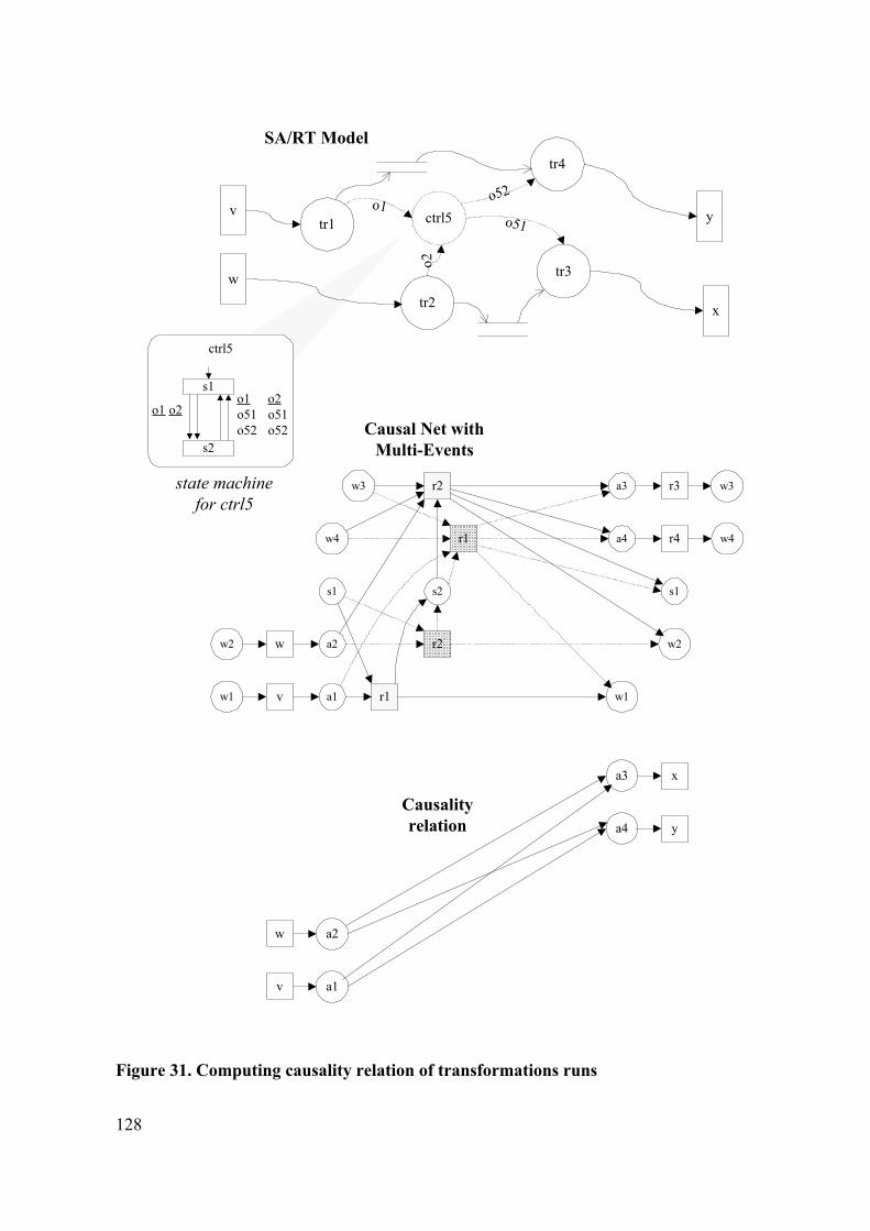
128
tr1
tr2
ctrl5
tr3
o1o51
v
w
o2
y
x
tr4
SA/RT Model
ctrl5
o1
s1
s2
o2
state machinefor ctrl5
r2
w1 v
w2
w1
a3
w2 w
s1
r2
r1
s2
r1
a1
a2
w3
s1
w4 a4
r3
w4r4
w3
Causal Net withMulti-Events
a1v
a3
w a2
a4
x
y
Causalityrelation
o1o51o52
o2o51o52
o52
Figure 31. Computing causality relation of transformations runs

129
6.3 Target Architecture Model
The target architecture or generic system architecture is defined by the possible types
and/or numbers of the system components, such as processor cores, memory, buses,
functional units (adders, multipliers) and data-path control unit and their possible
configurations. It is often called system platform, or computational platform. These
system components offer different kind of services that are needed for transformations to
progress their computation. Presence of the generic system structure in the form of the
target architecture very much simplifies the system architecture synthesis, and mapping
and scheduling, since the particular system architectures with mapped behavior are just
some specific instances of the generic system solution. In particular, the target
architecture model is needed for the assessment of the resources needed for
implementing the specified system behavior. Additionally some simplifying assumptions
are introduced that make these assessments possible at the early stages of design.
In the actual system, services can be requested for at any point in time. For this
reason resource-to-transformation allocation changes constantly. In this thesis, an
abstract model of the way the target architecture operates is used. As described earlier,
the approximate system behavior is modeled by the states distinguished and their
transitions. A data transformation is modeled by two to three states; the entire system
operation is described by combining the states of individual transformations and their
transitions. In the abstract model, it is assumed that the resource-to-transformation
allocation changes can only take place if they coincide with the system state transitions.
Although the abstract model does not precisely reflect the detailed system operation, it is
sufficient, at the early stages of design, for assessing the way resources should be
allocated to transformations.
The abstract model used can be described as a per system state transition lump sum
approach. Resource-to-transformation allocation changes that in fact take place during
the course of a transformation run are now summed up and put into effect already at the
start of the run. At the start of the transformation run, the resources required have already
been allocated and remain allocated for the period of the entire run. Possible changes in
the resource-to-transformation allocation scheme, which actually takes place during the
course of a transformation run, such as the release of resources, are only taken into
account after the transformation has completed its execution.
130
The target architecture involves a number of computational kernels that execute the
transformations. The computational kernel either has a data-flow architecture or some
processor core based architectures. It is assumed that the kernels are sub-systems of a
larger application-specific system-on-chip.
At the early design stages the actual kernel architecture may not be known. Basic
architectures are assumed for making the necessary assessments. These basic
architectures are generic and represent the actual architecture in an abstract way. They
are sufficiently detailed for making the assessments, required for the architectural and
mapping decisions.
The data-flow architecture adopted in this thesis involves a data-path with functional
units that implement arithmetic or logic functions. The control unit makes sure that data
is sent to the appropriate destination at the appropriate time. Furthermore, the data-flow
architecture has access to its local memory for storing data that need to be accessed
directly.
The computational kernels that are based on a processor core involve, besides the
computational core, a memory system. The memory systems are typically organized in a
hierarchical fashion. Memories at different hierarchy levels serve different purposes. In
this thesis, it is assumed that the memory hierarchy has two levels. The first level is used
for storing the data that can be accessed directly and is needed instantly by the processor
core. The second level of memory is used for the data that needs to be buffered over a
longer period of time. Such a memory scheme mimics the scheme as used in general-
purpose processors and digital signal processors.
In general-purpose processors, caches have been introduced in order to store the data
that can be readily accessed by the processor. The time to access a cache is relative short.
The cache memories are however more expensive compared to the memories that have
larger access times. For this reason the capacity of caches is limited. The data that does
not need to be accessed directly are stored (offloaded) in the slower main memory. The
main memory offers storage space at a relatively low cost. It can however not be directly
accessed by the processor core.
Instead of making the distinction between the data caches and main memory, a digital
signal processor core has the disposal of a local and a main memory. The local memory
has the same role as caches have for the general-purpose processors. The main memory

131
serves the purpose of buffering the data that is not needed directly by the processor core;
the buffered data needs to be loaded in the local memory first. Data transfers in the
digital signal processing systems are typically implemented using the direct memory
access (DMA) transfers.
Furthermore, the simplifying assumption is made that a transformation that has been
mapped onto a computational kernel can exclusively make use of the kernel’s resources.
Computational kernels only execute one transformation after another.
In the mapping and scheduling problem setting discussed in this thesis, the
computational kernels and memory capacity are the main resources that need to be
allocated to transformation runs. Their allocation determines the data transfers that need
to take place between the computational kernels, and the buses required.
Figure 34 gives an overview of the mapping and scheduling problem model as
considered in this thesis. The causal net that represents the system execution runs Figure
31 and the causality relations between the transformations runs is the starting point for
the mapping and scheduling problem. The transformation runs and data transfer make
requests for resources. The resources are provided by the target architecture. Resources
are shared by the transformation runs and need to be allocated and scheduled.
SYSTEM
tr1
tr2tr4
x
r1B
A
By
z
tr3r1
r2
Figure 32. Example of communication with data-flow and common variable
The local kernel memory is an important resource that is to be used as efficiently as
possible. Figure 32 shows a simple example with four transformations, tr1..tr4.
Transformations tr1 and tr2 communicate data A to each other using a discrete data-flow;
transformations tr3 and tr4 make use of the common variable B. Transformation tr2 is
independent of tr3 and tr4, which means that tr2 can be schedule before or after tr3 and

132
tr4. The order in which tr2..tr4 are scheduled has an impact on the amount of memory
resources used. This is shown in Figure 33. It can be easily seen that the first schedule
order is the best one. For larger examples, that involve multiple processor and inter-
processor communication, and large amounts of data transfer the schedule order is not so
obvious; the construction of a (sub-optimal) solutions then requires a search and
optimization process. Herein, besides the schedule order, the option of offloading data
can be considered. Offloading means that data that is still to be used by a subsequent
transformation is stored into main memory, in order to free local memory space. The data
is to be re-loaded before the next transformation uses the data. Freeing local kernel
memory, such that other message passing can make use of it happens at the cost of
additional delay in the execution of the transformation involved. This is shown in Figure
33, in the sub-plot at the bottom.
Relations and constraints exist between the transformations runs, resources request,
resources availability, resource allocation, and the target architecture. The composite of
all relations and constraints form the decision space. They are discussed subsequently.
ComputationalKernel
Local memory
tr1 tr2 tr3 tr4
A AB b
ComputationalKernel
Local memory
tr1 tr3 tr2 tr4
A A
Bb
ComputationalKernel
Local memory
tr2tr1 tr3 tr4
A AB b
Figure 33. Importance of schedule order for memory usage
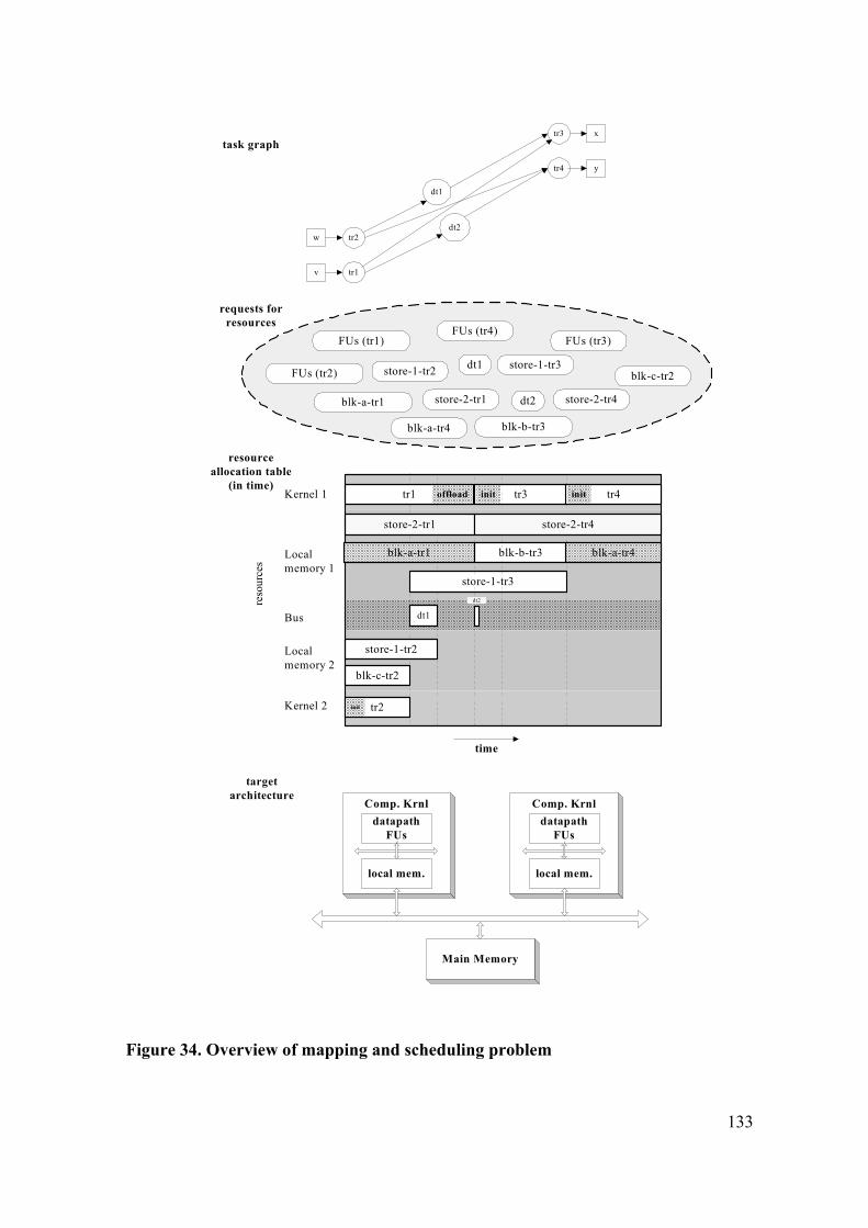
133
Main Memory
Comp. Krnldatapath
FUs
local mem.
Comp. Krnldatapath
FUs
local mem.
FUs (tr1)
tr2
tr3
store-1-tr3
dt1
blk-b-tr3
blk-c-tr2
tr1
store-1-tr2
store-2-tr1
Kernel 1
Localmemory 1
Bus
Localmemory 2
Kernel 2
FUs (tr4)FUs (tr3)
store-1-tr2 store-1-tr3dt1
blk-a-tr1
blk-a-tr4
store-2-tr1
time
reso
urce
s
requests forresources
task graph
resourceallocation table
(in time)
targetarchitecture
tr1v
tr3
w tr2
tr4
x
y
dt1
FUs (tr2) blk-c-tr2
store-2-tr4
blk-b-tr3
tr4
store-2-tr4
blk-a-tr1 blk-a-tr4
offload init
dt2
dt2
init
init
dt2
Figure 34. Overview of mapping and scheduling problem
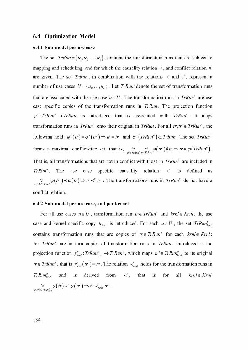
134
6.4 Optimization Model
6.4.1 Sub-model per use case
The set { }1 2, , , nTrRun tr tr tr= … contains the transformation runs that are subject to
mapping and scheduling, and for which the causality relation ≺ , and conflict relation #
are given. The set TrRun , in combination with the relations ≺ and # , represent a
number of use cases { }1, , mU u u= … . Let uTrRun denote the set of transformation runs
that are associated with the use case u U∈ . The transformation runs in uTrRun are use
case specific copies of the transformation runs in TrRun . The projection function
:u uTrRun TrRunϕ → is introduced that is associated with uTrRun . It maps
transformation runs in uTrRun onto their original in TrRun . For all , ' utr tr TrRun∈ , the
following hold: ( ) ( )' 'u utr tr tr trϕ ϕ= ⇒ = and ( )u uTrRun TrRunϕ ⊆ . The set uTrRun
forms a maximal conflict-free set, that is, ( ) ( )'
' #u
u
tr TrRuntr TrRuntr tr tr TrRunϕ ϕ
∈∈/∀ ∀ ⇒ ∈ .
That is, all transformations that are not in conflict with those in uTrRun are included in uTrRun . The use case specific causality relation u≺ is defined as
( ) ( ), '
' 'u
u
tr tr TrRuntr tr tr trϕ ϕ
∈∀ ⇒≺ ≺ . The transformations runs in uTrRun do not have a
conflict relation.
6.4.2 Sub-model per use case, and per kernel
For all use cases u U∈ , transformation run utr TrRun∈ and krnl Krnl∈ , the use
case and kernel specific copy krnltr is introduced. For each u U∈ , the set ukrnlTrRun
contains transformation runs that are copies of utr TrRun∈ for each krnl Krnl∈ ; utr TrRun∈ are in turn copies of transformation runs in TrRun . Introduced is the
projection function :u u ukrnl krnlTrRun TrRunγ → , which maps ' u
krnltr TrRun∈ to its original
utr TrRun∈ , that is ( )'ukrnl tr trγ = . The relation u
krnl≺ holds for the transformation runs in
ukrnlTrRun and is derived from u≺ , that is for all krnl Krnl∈
( ) ( ), '
' 'ukrnl
u ukrnl
tr tr TrRuntr tr tr trγ γ
∈∀ ⇒≺ ≺ .
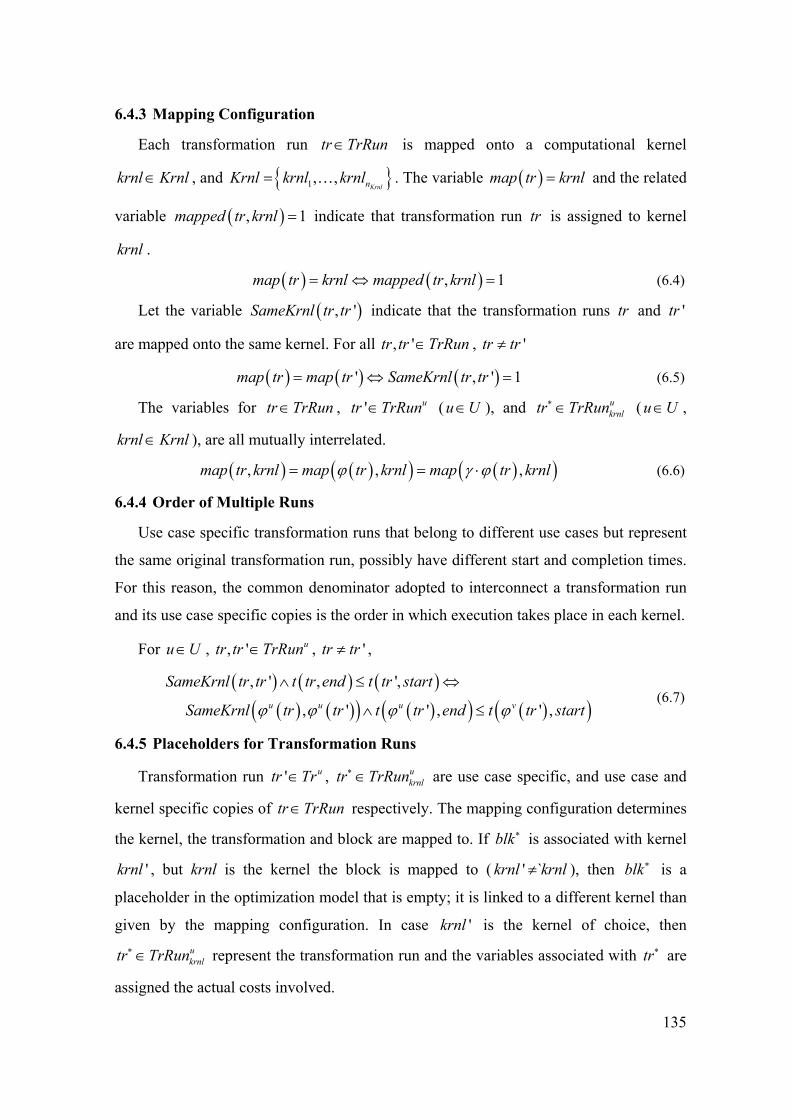
135
6.4.3 Mapping Configuration
Each transformation run tr TrRun∈ is mapped onto a computational kernel
krnl Krnl∈ , and { }1, ,KrnlnKrnl krnl krnl= … . The variable ( )map tr krnl= and the related
variable ( ), 1mapped tr krnl = indicate that transformation run tr is assigned to kernel
krnl .
( ) ( ), 1map tr krnl mapped tr krnl= ⇔ = (6.4)
Let the variable ( ), 'SameKrnl tr tr indicate that the transformation runs tr and 'tr
are mapped onto the same kernel. For all , 'tr tr TrRun∈ , 'tr tr≠
( ) ( ) ( )' , ' 1map tr map tr SameKrnl tr tr= ⇔ = (6.5)
The variables for tr TrRun∈ , ' utr TrRun∈ (u U∈ ), and ukrnltr TrRun∗ ∈ (u U∈ ,
krnl Krnl∈ ), are all mutually interrelated.
( ) ( )( ) ( )( ), , ,map tr krnl map tr krnl map tr krnlϕ γ ϕ= = ⋅ (6.6)
6.4.4 Order of Multiple Runs
Use case specific transformation runs that belong to different use cases but represent
the same original transformation run, possibly have different start and completion times.
For this reason, the common denominator adopted to interconnect a transformation run
and its use case specific copies is the order in which execution takes place in each kernel.
For u U∈ , , ' utr tr TrRun∈ , 'tr tr≠ ,
( ) ( ) ( )
( ) ( )( ) ( )( ) ( )( ), ' , ',
, ' ' , ' ,u u u v
SameKrnl tr tr t tr end t tr start
SameKrnl tr tr t tr end t tr startϕ ϕ ϕ ϕ
∧ ≤ ⇔
∧ ≤ (6.7)
6.4.5 Placeholders for Transformation Runs
Transformation run ' utr Tr∈ , ukrnltr TrRun∗ ∈ are use case specific, and use case and
kernel specific copies of tr TrRun∈ respectively. The mapping configuration determines
the kernel, the transformation and block are mapped to. If blk∗ is associated with kernel
'krnl , but krnl is the kernel the block is mapped to ( ' `krnl krnl≠ ), then blk∗ is a
placeholder in the optimization model that is empty; it is linked to a different kernel than
given by the mapping configuration. In case 'krnl is the kernel of choice, then ukrnltr TrRun∗ ∈ represent the transformation run and the variables associated with tr∗ are
assigned the actual costs involved.
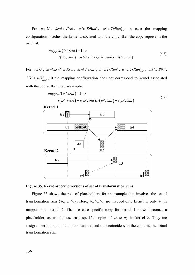
136
For u U∈ , krnl Krnl∈ , ' utr TrRun∈ , ukrnltr TrRun∗ ∈ in case the mapping
configuration matches the kernel associated with the copy, then the copy represents the
original.
( )', 1
( , ) ( ', ), ( , ) ( ', )
mapped tr krnl
t tr start t tr start t tr end t tr end∗ ∗
= ⇒
= = (6.8)
For u U∈ , ,krnl krnl Krnl∗ ∈ , krnl krnl∗≠ , ' utr TrRun∈ , ukrnl
tr TrRun ∗∗ ∈ , ' ublk Blk∈ ,
ukrnl
blk Blk ∗∗ ∈ , if the mapping configuration does not correspond to kernel associated
with the copies then they are empty.
( )
( ) ( ) ( ) ( )', 1
, ', , , ',
mapped tr krnl
t tr start t tr end t tr end t tr end∗ ∗
= ⇒
= = (6.9)
Kernel 1
Kernel 2
tr2
tr3
dt1
tr1 tr4offload init
tr1
tr3
tr4
tr2
dt2
Figure 35. Kernel-specific versions of set of transformation runs
Figure 35 shows the role of placeholders for an example that involves the set of
transformation runs { }1 4, ,tr tr… . Here, 1 3 4, ,tr tr tr are mapped onto kernel 1; only 2tr is
mapped onto kernel 2. The use case specific copy for kernel 1 of 2tr becomes a
placeholder, as are the use case specific copies of 1 3 4, ,tr tr tr in kernel 2. They are
assigned zero duration, and their start and end time coincide with the end time the actual
transformation run.
137
6.5 Modeling Constructs for Costs
6.5.1 Costs Constraints
The transformation runs take place at certain costs. There are different kinds of costs;
the set Param contains the different cost parameters considered. The costs can be
variable or fixed. Variable costs are the costs for the use of resources that can be directly
associated with the transformation runs deploying the resources. Resources that have
variable costs are non-renewable. Fixed costs are the costs for the shared resources used
by transformation runs. Resources that have fixed costs are renewable. That is, shared or
renewable resources can be continuously used without depletion. There is however the
restriction that resources cannot be used at the same time by multiple transformation
runs. The costs of a functional unit that is shared by transformation runs is accounted for
only once, and is not directly related to a particular transformation run. Power dissipation
on the other hand is an example of costs that can be directly associated with a
transformation run; the amount of power dissipated is not renewed.
Computational kernels can usually be implemented using a number of technologies,
which result in different performance and costs. In this thesis, it is assumed that the
choice of an implementation technology for a computational kernel has been made and
does not represent a decision in the optimization model. The system architect still can
consider different technologies using what-if analyses; the technology choice is however
a constant factor in the optimization model. When different technologies are used for the
kernels, then the costs and performance of a transformation run differ from kernel to
kernel.
Let { }1, ,TechnTech tech tech= … denote the set of implementation technologies
considered. For example, the variable ( ), ,cost par rsrc tech denotes the costs for
component rsrc (shared resource), using implementation technology tech with regard to
cost parameter type par . Because the implementation technology for krnl is known
beforehand, the cost for ( ), ,cost par rsrc krnl is a constant.
Let { }1, ,RsrcnRsrc fu fu= … denotes the multi-set of shared resources, which are
typically functional units or other hardware components. The set of shared resources
Rsrc is the disjoint-union of components that are used by the transformations. In order

138
to be able to distinguish between the components with the same type, the components are
assigned consecutive numbers starting with one. Each component is a distinct element in
the multi-set Rsrc . The numbering can be used, for example, to model the property that
if a transformation uses a component of some type with a certain number, then it also
uses the components of the same type that are lower numbered.
The implementation technology of the transformation run’s kernel determines the
costs for the transformation runs mapped to it. Let the variables ( )1cost par,tr,krnl …
( )Krnlncost par,tr,krnl represent the cost for transformation run tr with regard to costs
parameter par when it is mapped onto the kernel 1krnl … Krnlnkrnl , respectively. It is
assumed that estimates for these cost variables can be obtained and are known. In the
optimization model, these variables are constants.
The costs for a transformation run thus depend on the mapping configuration. For
this reason so called placeholders are introduced, which are kernel specific copies of
variables. Each placeholder represent the situation in which the transformation run that is
associated with the variable is actually mapped onto the kernel that is linked to the
placeholder. In this case the placeholder becomes relevant and represents the costs of the
original variable. Otherwise the placeholder is empty and set to an insignificant value.
The variables ( )varcost par,tr,krnl represent the (variable) costs of transformation run
tr with regard to parameter par in kernel krnl . The costs need only to be taken into
account if tr is actually mapped onto krnl , otherwise these costs are zero. For all
u U∈ , par Par∈ , utr TrRun∈ , krnl Krnl∈ , the following propositions hold:
( ) ( ) ( ), 1mapped tr krnl varcost par,tr,krnl = cost par,tr,krnl= ⇒ (6.10)
( ) ( ), 0 0mapped tr krnl varcost par,tr,krnl= ⇒ = (6.11)
The total variable costs for transformation runs for use case u U∈ that are mapped onto
kernel krnl is given by: ( ) ( ), , ,
utr TrRun
varcost par krnl varcost par tr krnl∈
= ∑ (6.12)
The fixed costs for the transformation runs that are mapped onto kernel krnl for use case
u U∈ are computed as follows. For the use case u, the set uRsrc is introduced which
contains copies of the for the use case u relevant resources in Rsrc . For use case u U∈ ,
139
utr TrRun∈ and ursrc Rsrc∈ , the variable ( , )use tr rsrc indicates that transformation run
tr makes use of shared resource rsrc. For all ursrc Rsrc∈ , let the variables
( ) ( ){ }, 1Use rsrc tr use tr rsrc= = render the set of transformation runs that deploys
shared resource rsrc . A component is used in kernel krnl if one of the transformation
run in ( )Use rsrc is mapped onto the kernel. ( ) ( )
( ), 1 , 1
tr Use rsrcused rsrc krnl mapped tr krnl
∈
= ⇔ ≥∑ (6.13)
Let the variables ( ), ,fixcost par rsrc krnl represent the costs of resource ursrc Rsrc∈ in
kernel krnl Krnl∈ . If resource rsrc is not deployed in kernel krnl , then the variable is
zero. Otherwise, the variable is set to the actual value of the costs. For u U∈ ,
par Par∈ , ursrc Rsrc∈ and krnl Krnl∈ , the following propositions hold. ( ) ( ) ( ), 1 , , , ,used rsrc krnl fixcost par rsrc krnl cost par rsrc krnl= ⇒ = (6.14)
( ) ( ), 0 , , 0used rsrc krnl fixcost par rsrc krnl= ⇒ = (6.15)
The total fixed costs with regard to par Par∈ for kernel krnl Krnl∈ is computed as
follows. ( ) ( )
ursrc Rsrc
fixcost par,krnl fixcost par,rsrc,krnl∈
= ∑ (6.16)
The sum ( ) ( ),varcost par krnl fixcost par,krnl+ renders the total costs with regard to
par for kernel krnl . Typically the total costs are limited, and the cost constraints are distributed over the
kernels. Let variables ( ),cap par krnl represent the kernel capacity for parameter par .
For par Par∈ , krnl Krnl∈ , the following constraints hold.
( ) ( ) ( ), ,varcost par krnl fixcost par,krnl cap par krnl+ ≤ (6.17)
The costs (variable and fixed) for the originals tr TrRun∈ are the same as for copies
' utr TrRun∈ , u U∈ , that is ( ) ( ) ( )'tr tr varcost par,tr',krnl varcost par,tr,krnlϕ = ⇒ =
The costs for the copies ukrnltr TrRun∗ ∈ , are the same as for the originals ( )trϕ γ ∗⋅ .
6.5.2 Transformation Run Delay
The transformation run delay is a somewhat special type of costs. Let the variables
( ),t tr start , ( ),t tr end and utr TrRun∈ represent the points in time at which
140
transformation run tr starts, respectively completes its execution (for use case u U∈ ).
Note that in case multiple use cases are involved, the variables ( ),t tr start and ( ),t tr end
for tr TrRun∈ cannot be given, since copies of tr in the different uTrRun , u U∈ may
have different start and completion times.
The transformation run execution delay consists of a number of components. Besides
the base execution delay, it possibly has additional delays for initialization/loading of
data and/or storing of data to offload the local kernel memory. The base execution delay
for a transformation run only reflect the ideal situation in which all the data the
transformation runs need, are present in the local kernel memory, at the start. No data
needs to be initialized, loaded into or offloaded from the local kernel memory.
Depending on the mapping configuration and schedule of the transformation runs
additional delays are incurred for these operations.
For each u U∈ , krnl Krnl∈ and ukrnltr TrRun∈ , the variables ( , )varcost delay tr ,
( ),t tr start and ( ),t tr end represent the total delay, start time and end time of tr
respectively. They are defined as follows. The variable ( , )varcost delay tr , ukrnltr TrRun∈
consists of the following components:
( , ) ( , ) ( , ) ( , )varcost delay tr varcost init tr varcost exec tr varcost offload tr= + + (6.18)
Note that tr is kernel specific which makes the variables above placeholders. The
variables are relevant and assigned the actual value if ( )trγ is mapped onto krnl .
Otherwise the variables associated with ukrnltr TrRun∈ are just empty placeholders.
The variable ( , )varcost exec tr , ukrnltr TrRun∈ gives the execution time needed for
( )trγ in kernel krnl , and is defined as follows:
( ) ( ) ( )( ) ( )
, , ,
, 0
mapped tr,krnl = 1 varcost exec tr cost exec tr krnl
mapped tr,krnl = 0 varcost exec tr
⇒ =⎧⎪⎨
⇒ =⎪⎩ (6.19)
The variable ( ),varcost exec tr only involves the base execution delay; the total
execution delay of tr further involves the additional delays that are related with the
blocks and stores associated with the transformation run. They are defined subsequently.
The base execution time for tr TrRun∈ is the same as for its copies in uTrRun and
141
ukrnlTrRun , in case they are not empty. The additional delays are however possible not
similar for the different use cases. For all krnl Krnl∈ , ukrnltr TrRun∈
( ) ( )( ) ( ), 1 , ,mapped tr krnl varcost exec tr varcost exec trϕ= ⇒ = (6.20)
The transformation run utr TrRun∈ completes its execution ( , )varcost delay tr after
( ),t tr start :
( ) ( ), , ( , )t tr end t tr start varcost delay tr= + (6.21)
6.6 Modeling Constructs for Local Memory Use
6.6.1 Blocks, Stores and Data-flows
The modeling constructs for blocks, stores and discrete data-flows are introduced in
this section. The computational kernels involve a local memory that can be directly
accessed by the kernel's data path or processor core. The model of the implementation
assumes that data passed on by blocks, store or data-flows are present in the local kernel
memory at the start of the associated transformation runs. Data can remain buffered for
subsequent transformation runs or offloaded at different costs. In the latter case, data
need to be re-loaded before a transformation run that requires the data can start. Also
data may need to be transferred between kernels, which is the when stores and data-flows
pass on data between transformations that are mapped onto different kernels. All these
aspects need to be considered and represented by the modeling constructs for the local
memory use.
6.6.2 Blocks
At the start of a transformation run, its data such as variables and instruction code
segments, need to be present in the local kernel memory. The mutual order of the
transformation runs determines whether data are possibly present in the local kernel
memory. If the transformation run is the first one in the schedule to use a block of a
certain type, then the block data needs to be initialized. Costs are involved for this
initialization, which for example entail computing the variables’ initial values or loading
them from the main memory into the local kernel memory. Similarly, the transformation
instruction code needs to be present in the local kernel memory at the start of the
transformation run.

142
Data is present in the local memory if the preceding transformation run that uses the
data, buffered the data. The local kernel memory capacity is however limited, in general.
Not all the data can remain in the local kernel memory in between transformation runs,
and some blocks need to be offloaded. In this case, data need to be temporarily stored in
the main memory, and loaded back into the local kernel memory at a later point in time.
Penalizing delays due to initialization and/or offloading of data need to be added to total
transformation run delay.
Blocks that have the same type and are mapped onto the same kernel have conjoining
lifetimes. These lifetimes jointly represent the lifetime of the data that is being referred
by the blocks. The data lifetime spans a period that can stretch multiple transformation
runs. During its lifetime, data are allotted slots in the local kernel memory, or are
buffered in the main memory.
6.6.3 Functions and Variables for Blocks
Let Blk denote the set of blocks in the system. The following functions and variables are
identified that are associated with a block blk Blk∈ .
• The function :tr Blk TrRun→ renders the transformation run that is associated
with block blk .
• The variable ( )type blk denotes the type of block blk Blk∈ .
• The function ( ):Blk TrRun Blk→ P renders the set of blocks that are associated
with transformation tr TrRun∈ .
• The function ( ):Tr Blk TrRun→ P renders the transformations runs that are
associated with blocks that have the same type as blk Blk∈ . That is,
( ) ( ) ( ) ( ){ }' , 'Tr blk tr blk blk Blk type blk type blk= ∈ = .
Similar to TrRun use case and kernel specific versions can be defined. The functions
:u u utr Blk TrRun→ , ( ):u u uBlk TrRun Blk→ P , and :u u ukrnl krnl krnltr Blk TrRun→ ,
( ):u u ukrnl krnl krnlBlk TrRun Blk→ P give the use case specific, and use case and kernel
specific versions, of the functions :tr Blk TrRun→ and ( ):Blk TrRun Blk→ P
respectively. The use case specific, and use case and kernel specific versions of the
143
function ( ):Tr Blk TrRun→ P is given by ( ):u u uTr Blk TrRun→ P , u U∈ and
( ):u u ukrnl krnl krnlTr Blk TrRun→ P , u U∈ , krnl Krnl∈ , respectively.
For all ublk Blk∈ , u U∈ and ' ukrnlblk Blk∈ , u U∈ , krnl Krnl∈ the variables
( ),t blk start , ( ),t blk end , ( )',t blk start , ( )',t blk end are defined. The variable
( ),t blk start denotes the start time at which memory slots are allotted to blk. The
variable ( ),t blk end denotes the time that memory slots are released, for use case u U∈ .
The use case and kernel specific versions are auxiliary variables and serve as
placeholders.
The costs of the initialization/loading operations of the blocks associated with
transformation run ukrnltr TrRun∈ , u U∈ , krnl Krnl∈ is given as follows. These
operations take place before the actual transformation run.
( )( )
( , )ukrnlblk Blk tr
varcost init tr varcost init,blk∈
= ∑ (6.22)
The store operations for offloading data are given as follows. These operations take place
after the actual transformation run.
( )( )
( , )ukrnlblk Blk tr
varcost offload tr varcost offload,blk∈
= ∑ (6.23)
The values for ( )varcost init,blk and ( )varcost offload,blk , ukrnlblk Blk∈ thus depend on
the mapping configuration, the ordering of the transformations runs, and on the decision
whether or not to offload certain blocks.
6.6.4 Mutual Order of Blocks
The mutual ordering positions of equally typed blocks are of importance for
determining whether initialization and/or offloading are of concern. For example, blocks
of a certain type that are scheduled first in a kernel always need to be initialized.
Auxiliary variables are introduced that indicate whether a transformation run is
scheduled first or last from a set of transformation runs, or succeed one another in a
computational kernel.
The variables ( ), ',succ tr tr krnl and ( ), ',prec tr tr krnl indicate whether
transformation run 'tr is succeeding or precede tr , and are assigned to kernel
144
krnl Krnl∈ . The variables ( ), 'SameKrnl tr tr have been introduced above;
( ), ',succ tr tr krnl and ( ), ',prec tr tr krnl are defined as follows.
( )( ) ( ) ( ) ( )( ), ', 1
, ', , ' '
succ tr tr krnl
map tr krnl t tr end t tr start SameKrnl tr tr tr tr
= ⇔
= ∧ ≤ ∧ ∨ = (6.24)
( )( ) ( ) ( ) ( )( ), ', 1
', , , ' '
prec tr tr krnl
map tr krnl t tr end t tr start SameKrnl tr tr tr tr
= ⇔
= ∧ ≤ ∧ ∨ = (6.25)
The variables ( ), ,cntsucc tr Tr krnl render the number of transformation runs in set Tr
that succeeds tr , and are assigned to kernel krnl . If tr Tr∈ then the count includes tr
itself. ( ) ( )
', , , ',
tr Trcntsucc tr Tr krnl succ tr tr krnl
∈
= ∑ (6.26)
Similarly, variables ( ), ,cntprec tr TrRun krnl are defined as follows. ( ) ( )
', , , ',
tr Trcntprec tr Tr krnl prec tr tr krnl
∈
= ∑ (6.27)
The variables ( ),cnt Tr krnl render the number of transformation runs in TrRun that are
assigned to kernel krnl . ( ), tr
tr TrRuncnt TrRun krnl map krnl
∈
= =∑ (6.28)
The variables ( ), ,first tr TrRun krnl indicate whether transformation run tr is scheduled
first among the transformation runs in Tr that are assigned to kernel krnl . ( ) ( ) ( ), , 1 , , ,first tr Tr krnl cntsucc tr Tr krnl cnt Tr krnl= ⇔ = (6.29)
Similarly, the variables ( ), ,last tr Tr krnl indicate whether transformation run tr is
scheduled last. ( ) ( ) ( ), , 1 , , ,last tr Tr krnl cntprec tr Tr krnl cnt Tr krnl= ⇔ = (6.30)
Let the variable ( ), ', ,firstprec tr tr Tr krnl indicate that transformation run 'tr directly
precedes tr in kernel krnl .
( )
( ) ( ), ', , 1
, , ', , 1
firstprec tr tr Tr krnl
cntprec tr Tr krnl cntprec tr Tr krnl
= ⇔
− = (6.31)
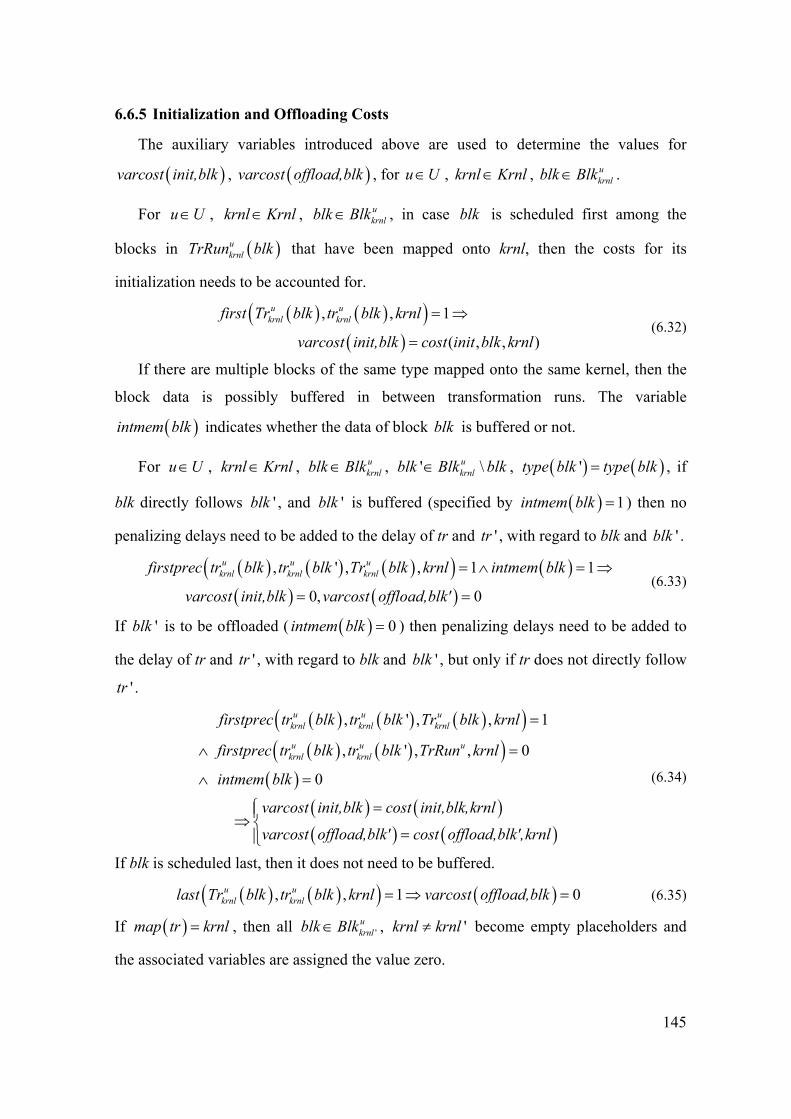
145
6.6.5 Initialization and Offloading Costs
The auxiliary variables introduced above are used to determine the values for
( )varcost init,blk , ( )varcost offload,blk , for u U∈ , krnl Krnl∈ , ukrnlblk Blk∈ .
For u U∈ , krnl Krnl∈ , ukrnlblk Blk∈ , in case blk is scheduled first among the
blocks in ( )ukrnlTrRun blk that have been mapped onto krnl, then the costs for its
initialization needs to be accounted for.
( ) ( )( )
( ), , 1
( , , )
u ukrnl krnlfirst Tr blk tr blk krnl
varcost init,blk cost init blk krnl
= ⇒
= (6.32)
If there are multiple blocks of the same type mapped onto the same kernel, then the
block data is possibly buffered in between transformation runs. The variable
( )intmem blk indicates whether the data of block blk is buffered or not.
For u U∈ , krnl Krnl∈ , ukrnlblk Blk∈ , ' \u
krnlblk Blk blk∈ , ( ) ( )'type blk type blk= , if
blk directly follows 'blk , and 'blk is buffered (specified by ( ) 1intmem blk = ) then no
penalizing delays need to be added to the delay of tr and 'tr , with regard to blk and 'blk .
( ) ( ) ( )( ) ( )( ) ( )
, ' , , 1 1
0, 0
u u ukrnl krnl krnlfirstprec tr blk tr blk Tr blk krnl intmem blk
varcost init,blk varcost offload,blk'
= ∧ = ⇒
= = (6.33)
If 'blk is to be offloaded ( ( ) 0intmem blk = ) then penalizing delays need to be added to
the delay of tr and 'tr , with regard to blk and 'blk , but only if tr does not directly follow
'tr .
( ) ( ) ( )( )( ) ( )( )
( )( ) ( )( ) ( )
, ' , , 1
, ' , , 0
0
u u ukrnl krnl krnl
u u ukrnl krnl
firstprec tr blk tr blk Tr blk krnl
firstprec tr blk tr blk TrRun krnl
intmem blk
varcost init,blk cost init,blk,krnl
varcost offload,blk' cost offload,blk',krnl
=
∧ =
∧ =
=⇒
=
⎧⎪⎨⎪⎩
(6.34)
If blk is scheduled last, then it does not need to be buffered.
( ) ( )( ) ( ), , 1 0u ukrnl krnllast Tr blk tr blk krnl varcost offload,blk= ⇒ = (6.35)
If ( )map tr krnl= , then all 'ukrnlblk Blk∈ , 'krnl krnl≠ become empty placeholders and
the associated variables are assigned the value zero.

146
( )( )
( ) ( ), 0
0, 0
ukrnlmapped tr blk krnl
varcost init,blk varcost offload,blk
= ⇒
= = (6.36)
6.6.6 Memory Allocation for Blocks
For u U∈ , krnl Krnl∈ , ukrnlblk Blk∈ , if block blk is scheduled first among similarly
typed blocks in kernel krnl, then the start of the memory allocation to block blk coincides
with the start of its transformation run.
( ) ( )( ) ( ) ( )( ), , 1 , ,u u ukrnl krnl krnlfirst tr blk Tr blk krnl t blk start t tr blk start= ⇒ = (6.37)
The end of memory allocation to block ukrnlblk Blk∈ , u U∈ , krnl Krnl∈ always
coincides with the end of its transformation run. This applies also for ukrnlblk Blk∈ and
ukrnltr TrRun∈ that are empty placeholders.
( ) ( )( ), ,ukrnlt blk end t tr blk end= (6.38)
For u U∈ , krnl Krnl∈ , ukrnlblk Blk∈ , ' \u
krnlblk Blk blk∈ , ( ) ( )'type blk type blk= , if
block blk directly follows 'blk , and the data has been buffered for block blk in local
memory ( ( ) 1intmem blk = ), then the lifetimes of blk and 'blk are joined.
( ) ( ) ( )( ) ( )
( ) ( )( ) ( ) ( )( ), ' , , 1 1
, ' , , ', ' ,
u u ukrnl krnl krnl
u ukrnl krnl
firstprec tr blk tr blk Tr blk krnl intmem blk
t blk start t tr blk end t blk end t tr blk end
= ∧ = ⇒
= = (6.39)
If it is not buffered and tr does not directly follow 'tr , then the memory is released as
soon as ( )'ukrnltr blk completes its run, and is again allocated at the start of ( )u
krnltr blk .
( ) ( ) ( )( )( ) ( )( )
( )( ) ( )( )( ) ( )( )
, ' , , 1
, ' , , 0
0
, ,
', ' ,
u u ukrnl krnl krnl
u u ukrnl krnl
ukrnl
ukrnl
firstprec tr blk tr blk Tr blk krnl
firstprec tr blk tr blk TrRun krnl
intmem blk
t blk start t tr blk start
t blk end t tr blk end
=
∧ =
∧ =
⎧ =⎪⇒ ⎨=⎪⎩
,
(6.40)
If it is not buffered but tr directly follows 'tr , then the lifetimes of blk and 'blk are
joined.

147
( ) ( ) ( )( )( ) ( )( )
( )( ) ( )( )
( ) ( )( )
, ' , , 1
, ' , , 1
0
, ' ,
', ' ,
u u ukrnl krnl krnl
u u ukrnl krnl
ukrnl
ukrnl
firstprec tr blk tr blk Tr blk krnl
firstprec tr blk tr blk TrRun krnl
intmem blk
t blk start t tr blk end
t blk end t tr blk end
=
∧ =
∧ =
⎧ =⎪⇒ ⎨=⎪⎩
,
(6.41)
The memory of a block that is scheduled last is released as soon as its transformation run
is completed. This property is also modeled by (6.38).
( ) ( )( ) ( ) ( )( ), , 1 , ,u u ukrnl krnl krnllast Tr blk tr blk krnl t blk end t tr blk end= ⇒ = (6.42)
Block ' ukrnlblk Blk∈ is a use case kernel specific copy of blk Blk∈ . If block 'blk is not
mapped onto kernel krnl, it becomes a placeholder. The block and its related variables
are set to default values.
( )( )
( ) ( )( ) ( ) ( )( ), 0
, , , , ,
ukrnl
u ukrnl krnl
mapped tr blk krnl
t blk end t tr blk end t blk start t tr blk end
= ⇒
= = (6.43)
6.6.7 Stores and Data-flows
Stores and data-flows are modeling element in a SA/RT model that are represented
explicitly graphically. For each store or data-flow, source and destination transformations
are involved. For the optimization model, it is assumed that stores and data-flows only
have one source and one destination. Point-to-n-point message passing is implemented
by n two-way message passing. The source transformation run produces the data. The
data is preferably buffered until the destination transformation run has read the data. The
destination transformation is possibly mapped onto a different kernel than the source
transformation. In this case, the data needs to be transferred across kernel boundaries,
before it is buffered in the local kernel memory of the destination transformation. In case
both the source and destination transformations are mapped onto the same kernel, the
data can be buffered in the main memory and free up capacity in the local kernel
memory.
In the optimization model, individual objects str Str∈ are introduced to represent the
occasions at which stores or data-flows are used for message passing,. Such an object
involves two parts, a source ( )str src and destination ( )str dest part. Furthermore,
transfer objects ( )tf str for each str Str∈ are introduced. They represent the data
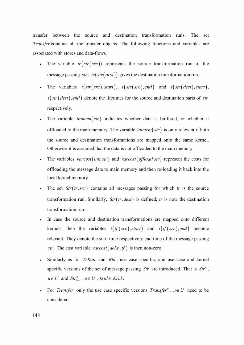
148
transfer between the source and destination transformation runs. The set
Transfer contains all the transfer objects. The following functions and variables are
associated with stores and data-flows.
• The variable ( )( )tr str src represents the source transformation run of the
message passing str ; ( )( )tr str dest gives the destination transformation run.
• The variables ( )( ),t str src start , ( )( ),t str src end and ( )( ),t str dest start ,
( )( ),t str dest end denote the lifetimes for the source and destination parts of str
respectively.
• The variable ( )intmem str indicates whether data is buffered, or whether it
offloaded to the main memory. The variable ( )intmem str is only relevant if both
the source and destination transformations are mapped onto the same kernel.
Otherwise it is assumed that the data is not offloaded to the main memory.
• The variables ( )varcost init,str and ( )varcost offload,str represent the costs for
offloading the message data to main memory and then re-loading it back into the
local kernel memory.
• The set ( ),Str tr src contains all messages passing for which tr is the source
transformation run. Similarly, ( ),Str tr dest is defined; tr is now the destination
transformation run.
• In case the source and destination transformations are mapped onto different
kernels, then the variables ( )( ),t tf src start and ( )( ),t tf src end become
relevant. They denote the start time respectively end time of the message passing
str . The cost variable ( )varcost delay,tf is then non-zero.
• Similarly as for TrRun and Blk , use case specific, and use case and kernel
specific versions of the set of message passing Str are introduced. That is uStr ,
u U∈ and ukrnlStr , u U∈ , krnl Krnl∈ .
• For Transfer only the use case specific versions uTransfer , u U∈ need to be
considered.
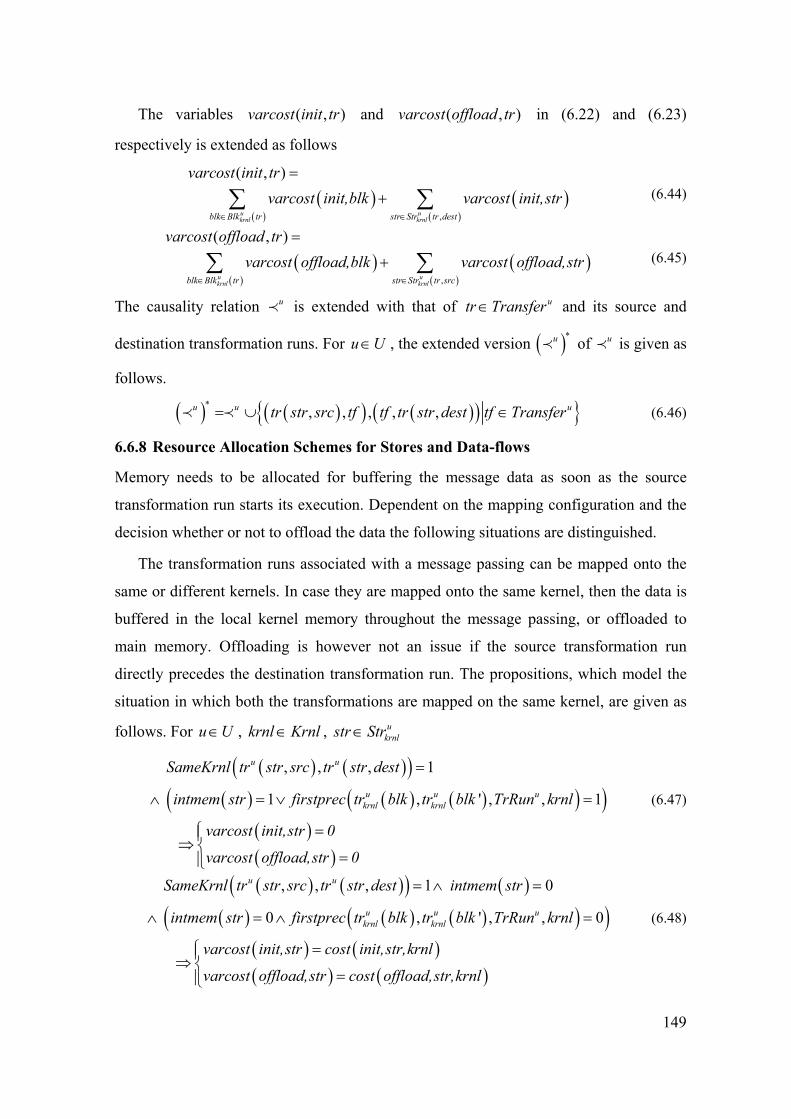
149
The variables ( , )varcost init tr and ( , )varcost offload tr in (6.22) and (6.23)
respectively is extended as follows
( )( )
( )( ),
( , )
u ukrnl krnlblk Blk tr str Str tr dest
varcost init trvarcost init,blk varcost init,str
∈ ∈
=
+∑ ∑ (6.44)
( )( )
( )( ),
( , )
u ukrnl krnlblk Blk tr str Str tr src
varcost offload trvarcost offload,blk varcost offload,str
∈ ∈
=
+∑ ∑ (6.45)
The causality relation u≺ is extended with that of utr Transfer∈ and its source and
destination transformation runs. For u U∈ , the extended version ( )u ∗≺ of u≺ is given as
follows.
( ) ( )( ) ( )( ){ }, , , , ,u u utr str src tf tf tr str dest tf Transfer∗
= ∪ ∈≺ ≺ (6.46)
6.6.8 Resource Allocation Schemes for Stores and Data-flows
Memory needs to be allocated for buffering the message data as soon as the source
transformation run starts its execution. Dependent on the mapping configuration and the
decision whether or not to offload the data the following situations are distinguished.
The transformation runs associated with a message passing can be mapped onto the
same or different kernels. In case they are mapped onto the same kernel, then the data is
buffered in the local kernel memory throughout the message passing, or offloaded to
main memory. Offloading is however not an issue if the source transformation run
directly precedes the destination transformation run. The propositions, which model the
situation in which both the transformations are mapped on the same kernel, are given as
follows. For u U∈ , krnl Krnl∈ , ukrnlstr Str∈
( ) ( )( )( ) ( ) ( )( )( )
( )( )
, , , 1
1 , ' , , 1
u u
u u ukrnl krnl
SameKrnl tr str src tr str dest
intmem str firstprec tr blk tr blk TrRun krnl
varcost init,str 0
varcost offload,str 0
=
∧ = ∨ =
=⎧⎪⇒ ⎨=⎪⎩
(6.47)
( ) ( )( ) ( )
( ) ( ) ( )( )( )( ) ( )( ) ( )
, , , 1 0
0 , ' , , 0
u u
u u ukrnl krnl
SameKrnl tr str src tr str dest intmem str
intmem str firstprec tr blk tr blk TrRun krnl
varcost init,str cost init,str,krnl
varcost offload,str cost offload,str,krnl
= ∧ =
∧ = ∧ =
=⎧⎪⇒ ⎨=⎪⎩
(6.48)
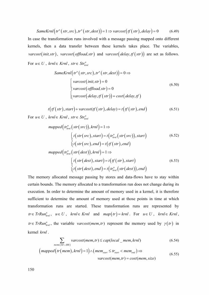
150
( ) ( )( ) ( )( ), , , 1 , 0u uSameKrnl tr str src tr str dest varcost tf str delay= ⇒ = (6.49)
In case the transformation runs involved with a message passing mapped onto different
kernels, then a data transfer between these kernels takes place. The variables,
( )varcost init,str , ( )varcost offload,str and ( )( ),varcost delay tf str are set as follows.
For u U∈ , krnl Krnl∈ , ukrnlstr Str∈
( ) ( )( )( )( )
( )( ) ( )
, , , 0
0
0
, ,
u uSameKrnl tr str src tr str dest
varcost init,str
varcost offload,str
varcost delay tf str cost delay tf
= ⇒
⎧ =⎪⎪ =⎨⎪
=⎪⎩
(6.50)
( )( ) ( ) ( )( ), ( , ) ,t tf str start varcost tf str delay t tf str end+ = (6.51)
For u U∈ , krnl Krnl∈ , ukrnlstr Str∈
( )( )( )( )( ) ( )( )( )( )( ) ( )( )
, 1
, ,
, ,
ukrnl
ukrnl
mapped tr str src krnl
t str src start t tr str src start
t str src end t tf str end
= ⇒
⎧ =⎪⎨
=⎪⎩
(6.52)
( )( )( )( )( ) ( )( )( )( ) ( )( )( )
, 1
, ,
, ,
ukrnl
ukrnl
mapped tr str dest krnl
t str dest start t tf str start
t str dest end t tr str dest end
= ⇒
⎧ =⎪⎨
=⎪⎩
(6.53)
The memory allocated message passing by stores and data-flows have to stay within
certain bounds. The memory allocated to a transformation run does not change during its
execution. In order to determine the amount of memory used in a kernel, it is therefore
sufficient to determine the amount of memory used at those points in time at which
transformation runs are started. These transformation runs are represented by ukrnltr TrRun∈ , u U∈ , krnl Krnl∈ and ( )map tr krnl= . For u U∈ , krnl Krnl∈ ,
ukrnltr TrRun∈ , the variable ( , )varcost mem tr represent the memory used by ( )trγ in
kernel krnl .
( )
( , ) ( _ , )mem Str Blk
varcost mem tr cap local mem krnl∈ ∪
≤∑ (6.54)
( )( )( ) ( ), 1
( , ) ( , )start start endmapped tr mem krnl mem tr mem
varcost mem tr cost mem size
= ∧ ≤ < ⇒
= (6.55)
151
( )( )( ) ( ) ( ), 1
( , ) 0start start start endmapped tr mem krnl tr < mem tr > mem
varcost mem tr
≠ ∨ ∨ ⇒
= (6.56)
Figure 34 shows an example of the use of blocks and stores. Three block types and
two stores are distinguished: blk-a, blk-b and blk-c, and store-1 and store-2. Blk-a
involves two transformation runs that are mapped onto the same kernel. Intermediate
transformation runs in between them exist. These are conditions under which Blk-a can
be offloaded. Blk-a is offloaded, which causes an additional delay in tr1 (offloading) and
tr4 (initialization). These additional delays are to be added to the ideal transformation
run’s ideal execution delay. Blk-b and blk-c both cause additional delay since they are
the first block used within their kernel. The data transfer for store-1 is relevant since the
transformations associated are mapped onto different kernels. The data transfer for store
2 is however a placeholder.
6.7 Modeling Constructs for Scheduling Order
6.7.1 Precedence Constraints
Transformation runs that are mapped onto the same kernel are executed one after the
other and their executions are non-overlapping. The following propositions are
introduced in order to model the non-overlap constraints. For u U∈ , and , ' utr tr TrRun∈
( ) ( ) ( )( ) ( ) ( )( ), ' 1 , ', ', ,SameKrnl tr tr t tr end t tr start t tr end t tr start= ⇒ ≤ ∨ ≤ (6.57)
Assumed is that data transfers cannot take place simultaneously. This is modeled as
follows. For u U∈ , and , ' utf tf Transfer∈
( ) ( )( ) ( ) ( )( ), ', ', ,t tf end t tf start t tf end t tf start≤ ∨ ≤ (6.58)
For a use case u U∈ , the causality relation between the transformation runs
, ' utr tr TrRun∈ is given by u≺ . This has been extended to ( )u ∗≺ in order to include the
data transfers and its causality relation with transformation runs. Let u u uTrTf TrRun Transfer= ∪ contain both transformation runs and data transfer for use
case u U∈ . The causality relation ( )u ∗≺ renders the following constraints. For
, ' utrtf trtf TrTf∈ , ( ) ( ), ' utrtf trtf∗
∈ ≺ the following proposition hold:
( ) ( ), ',t trtf end t trtf start≤ (6.59)
152
6.7.2 Main Memory Buffering Policy
The data passed on by blocks, stores or data-flows is either buffered in the local
kernel memory or in the main memory in-between transformation runs. Data that is not
present in the local kernel memory at the start of a transformation run either belongs to a
block of a certain type that is scheduled first in the kernel, or it has been offloaded by a
preceding transformation run. The data first needs to be loaded into the local kernel
memory before the transformation run can starts its execution.
A policy can be used to lay down rules when to buffer data and when to keep it in the
local kernel memory. For example, the last-in-first-out scheduling policy is modeled as
follows. The principle here is to prefer to keep the more recently used data in the local
kernel memory and offload the older data. It is modeled as follows.
Introduced is the notion of the potential buffering period, which is the time that data
possibly remains in the local memory without its transformation run being active. Two
data objects that make up a message passing have a potential buffering period if their
transformations runs do not directly succeed each other, and there is no data object of
similar type in between them.
Let 1data , 1data∗ make up a message passing by blocks, stores or data-flows. The set
1Data contains data objects that have the same type. Then there is a potential buffering
period for 1data and 1data∗ if the following proposition hold. The potential buffering
period starts at ( )( )1 ,t tr data end and ends at ( )( )1 ,t tr data start∗ .
( ) ( )( )( ) ( )( )
1 1 1
1 1
, , , 1
, , , 0
firstprec tr data tr data Data krnl
firstprec tr data tr data TrRun krnl
∗
∗
=
∧ = (6.60)
Let 2data , 2data∗ make up another message passing, which potential buffering period
starts at ( )( )2 ,t tr data end and ends at ( )( )2 ,t tr data start∗ . Let the second potential
buffering period be older than the first one, and overlapping. This means that the start of
the first potential buffering period lies within the second potential period.
If the data remains in the local memory in the second potential buffering period, then
it needs to remain in the local kernel memory in the first potential buffering period, since
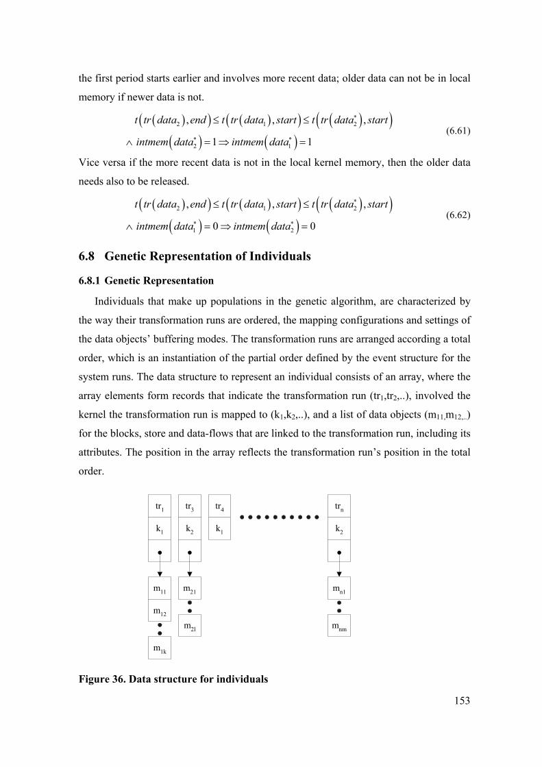
153
the first period starts earlier and involves more recent data; older data can not be in local
memory if newer data is not.
( )( ) ( )( ) ( )( )
( ) ( )2 1 2
2 1
, , ,
1 1
t tr data end t tr data start t tr data start
intmem data intmem data
∗
∗ ∗
≤ ≤
∧ = ⇒ = (6.61)
Vice versa if the more recent data is not in the local kernel memory, then the older data
needs also to be released.
( )( ) ( )( ) ( )( )
( ) ( )2 1 2
1 2
, , ,
0 0
t tr data end t tr data start t tr data start
intmem data intmem data
∗
∗ ∗
≤ ≤
∧ = ⇒ = (6.62)
6.8 Genetic Representation of Individuals
6.8.1 Genetic Representation
Individuals that make up populations in the genetic algorithm, are characterized by
the way their transformation runs are ordered, the mapping configurations and settings of
the data objects’ buffering modes. The transformation runs are arranged according a total
order, which is an instantiation of the partial order defined by the event structure for the
system runs. The data structure to represent an individual consists of an array, where the
array elements form records that indicate the transformation run (tr1,tr2,..), involved the
kernel the transformation run is mapped to (k1,k2,..), and a list of data objects (m11,m12,..)
for the blocks, store and data-flows that are linked to the transformation run, including its
attributes. The position in the array reflects the transformation run’s position in the total
order.
tr1 tr3 tr4 trn
k1 k2 k2k1
m11
m12
m1k
m21
m2l
mn1
mnm
Figure 36. Data structure for individuals

154
As discussed earlier, a distinction is made between the individuals’ space and the
solutions’ space. Individuals form the base for solutions. In order to obtain values for
criteria and objectives, the individual need to be decoded and evaluated further.
6.9 Decoding Algorithm
The solution that embodies an individual is constructed as follows. Hereby the
individual is described by its data structure, and the transformation runs and the causality
and conflict relation are given. The solutions are decomposed into partial solutions, that
each relates with a use case u U∈ . Each partial solution consists of
1. the mapping configuration for the transformation runs;
2. the start and end times for the transformation runs;
3. the start and end times for the data transfers;
4. the buffering modes for the data objects.
The partial solution that is related to u U∈ renders a point ( )1 , ,u u umq q q= … in the
objective space. Full solutions involve m U× objectives since there are U use cases.
MADM methods are used to model and solve the problem of ranking and sorting the
solutions.
The first step for obtaining the partial solution for use case u U∈ is to construct the
task graphs ( ),u u uG V E= . The set of nodes represent the transformation runs and data
transfers for message passing using stores and data-flows. The nodes have attributes. The
edges represent the causality relation between the node objects.
The second step is to determine the order in which the transformation runs are
executed in each of the computational kernels, for the use cases distinguished. The total
order of the transformation runs, in combination with the mapping configuration,
provides sufficient information to determine the order of the transformation runs for each
of the computational kernels.
The third step involves determining the execution delays for the transformation runs
and the data transfers. The mapping configuration contains the necessary information in
order to determine the complete transformation run delay, including the additional
penalty delays for handling blocks, stores, and data-flows, since the order of the
155
transformation runs per computational kernel and the settings for the data objects buffer
modes are known.
The execution delays for the transformation runs and data transfers have been
determined in the previous step. The start and end times of the transformation runs and
data transfers are computed using as-soon-as-possible scheduling. The scheduling
process operates as follows. Let ≺ denote the overall individual’s total order for the
transformation runs, and u≺ be the causality relation as specified by the data and control
flow between the transformation runs and data transfers. Let Open and Closed denote
the sets of nodes in the task graph that are not scheduled respectively still need to be
scheduled. For each scheduling step, a node v Open∈ is chosen such that all the nodes
that precedes v are included in Closed , all the nodes that succeeds v are in Open and
the conditions mv v= , 1 1 1m m m nO v v v v v− += … … , and the property ( ) ( )1 1u
i i i iv v v v+ +⇒≺ ≺
holds. That is, if the partial order relation u≺ holds between transformation runs, then the
total order relation also hold.
In case there is a data or control flow relation between v and nodes that already have
been scheduled (i.e. nodes are in Closed), then v start time is set to the maximum of the
end times of these scheduled nodes. In case the last scheduled node that has been mapped
onto the same computational kernel or bus as v has a greater end time, then v start time
is set to this greater value. The data transfers’ start and en time are based on the start and
end times of the transformation runs.
The start and end times of transformation runs and data transfer makes it possible to
determine the lifetimes of the data objects for stores, blocks and data-flows. The memory
requirements for the various data objects are then known. The memory requirements for
a kernel at a certain point in time consist of the data objects that are alive at that time.
Solutions are evaluated based on criteria such as makespan (last transformation run
end time), maximal memory use for each of the kernels, average memory use over time
for each of the kernels, amount of data transfers. These criteria represent the solution in
objective space, and can be obtained by decoding the individuals.
156
6.10 Selection Operator
6.10.1 Enhanced Non-dominated Sorting
In this thesis, refinements for the non-dominated sorting method are introduced, and
the enhanced version is used for solving the mapping and scheduling problem. The
refinement consists of also making the distinction between dominating and non-
dominating alternatives, additional to the distinction made between dominated and non-
dominated alternatives. At each step i , let iY denote the set of alternatives that need to
be screened. Let iD render the dominance relation for iY . The range of iD is given by
the set ( ) ( ){ }range ,i iD y x y D= ∈ ; the domain of iD is the set
( ) ( ){ }dom ,i iD x x y D= ∈ .
The variable ( )rngi i ind Y D= − renders the set of non-dominated alternatives of iY .
At each separating step, the alternatives are grouped into four variable sets instead of two
as is the case for regular non-dominated sorting. The variable sets are computed as
follows, and represent the different categories.
• Non-dominated and dominating: ( )domi i indd nd D= ∩
• Non-dominated and non-dominating: ( )/domi i indnd nd D=
• Dominated and dominating: ( ) ( )=ran domi i idd D D∩
• Dominated and non-dominating: ( )rani i idnd nd D= ∩
The alternatives in indd are given a higher rank than in indnd . In turn the
alternatives in indnd are given a higher rank those in i idd dnd∪ . The set to be screened
at step 1i + is 1i i iY dd dnd+ = ∪ . At the last step ndd and ndnd are empty sets; the
alternatives in dd are given a higher rank than those in dnd .
6.10.2 Imprecise Assessments
The preference modeling methods discussed above all assume that assessments of
solutions render crisp values. It could well be that the assessment values are imprecise. In
this thesis, some of the assessments are given as an interval instead of a crisp number;
the assessment of solution x for criterion iq is given by the interval
157
( ) ,min ,max,i i iq q q⎡ ⎤= ⎣ ⎦x xx (6.63)
Besides the interval boundaries, the decision maker can provide additional information
for modeling the preferences. For example, points in the assessment interval are assigned
values. These values indicate the possibility of the points they are assigned to, to be the
actual assessment. The points in combination with the possibilities represent fuzzy
numbers. A number of methods have been proposed for fuzzy multi-attribute decision-making
[23]. These methods have been developed with a generic problem setting in mind. The
problem setting in this thesis is more restricted. The general case in which the criterion
assessment can be any fuzzy number is not considered in this thesis. The assumption is
made that the possibility for the actual assessment value of criterion iq to take on the
interval boundary values ,miniq x or ,maxiq x is practically zero. Objectives are in conflict; the
values of a compromise solution are more likely to have the value ( ),max ,min 2i iq q−x x , and
1, ,i m= … rather than to take one the values at the end of the range. In this thesis, the
median interval points ( ),max ,minˆ 2i i iq q q= −x x x , 1, ,i m= … are assigned the possibility
level one; the boundary points ,miniq x are ,maxiq x assigned the possibility level zero. The
values are linearly increasing, respectively decreasing from ,miniq x to ˆiq x , and from ˆiq x to
,maxiq x . The preference structure for criterion iq with imprecise assessments is defined as
follows.
( ) ( )( ) ( )( ) ( )
,max ,min ,max ,min ,max ,min
,max ,min ,max ,min ,max ,max ,min ,max
,max ,min ,max ,min ,max ,max ,min ,max
, and
, and ,
, and ,
i i i i i i
i i i i i i i i i
i i i i i i i i
q q q q q q
P q q q q q q q q
q q q q q q q q
⎧ + ≥ + ≥⎪⎪⇔ + = + ≥ >⎨
+ = + > ≥⎩
x x y y x y
x x y y y x x y
x x y y y x x y
x y⎪⎪
(6.64)
i i iI P P⇔ ∧x y x y y x (6.65)
The dominance relation for criteria with imprecise assessments is then defined as
follows.

158
Definition 49. Dominance Relation with Imprecision
The dominance relation “alternative x dominates y ” ( Dx y ) is defined as
{ }1, , 1, ,. .
j i ij m i mD P P I
∈ =⇔ ∃ ∧ ∀ ∨ /
… …x y x y x y x y
(6.66)
6.11 Crossover and Mutation Operator
Use of a genetic algorithm requires the definition of crossover and mutation operators
specific to the structure used to represent the individual. Individuals are characterized by
their orderings of the transformation runs, mapping configurations and settings of the
data objects’ buffering modes. The genetic algorithm always enforces the precedence
constraints. Only resource and/or temporal constraints may be violated. A repair
algorithm can be used in order to obtain a consistent set of the data objects’ buffering
mode settings. After repairs these settings comply with the constraints for the data
objects. Another possibility is to defer the decision on the buffering mode settings until
after the search. This means that the search algorithm has to deal with imprecise
assessments of the criteria. The crossover operator and the mutation operator include two
parts: one for the total ordering of the transformation runs, and one for the mapping
configuration.
6.11.1 Crossover of Total Order
The crossover operator for the ordering component is implemented as follows. Let pi
and qi are two individuals that have been draw at random from the mating pool. Their
total orderings are given by the ordered lists ,1 ,2 ,p p p nt t t… and ,1 ,2 ,q q q nt t t… respectively.
The precedence relation of these ordered lists are given by p≺ and q≺ respectively
(pruned form). The crossover operator selects a crossing point r at random and creates
two new individuals 1c
i and 2ci . Their total orderings are given by the ordered lists
1 1 1 1,1 ,2 , ,c c c r c nt t t t… … and 2 2 2 2,1 ,2 , ,c c c r c nt t t t… … respectively. Let { },1 ,2 ,, ,r
p p p p rJ t t t= … and
{ },1 ,2 ,, ,rq q q q rJ t t t= … are the sets containing the first r elements of the ordered lists that
belongs to the individuals pi and qi respectively. Also let
{ } { },1 ,2 , ,1 ,2 ,, , , , , ,p p p n q q q nJ t t t t t t= =… … . The following propositions hold for the total

159
ordering of the newly created individuals. The first r positions are copied from pi ’s
ordered list. The positions from 1r + to n consist of the transformation runs are not
included in rpJ and are ordered according the overall ordering of qi .
( ) { } ( )1 1 1
1 1 1 1 1 1
,1 ,2 , ,1 ,2 ,
, 1 , , 1 , , , 1\
, , \ , , , , ,rp
c c c r p p p r
rc r c n p c r c n c r i c r i q
j J J
t t t t t t
t t J J j t t t i ++ + + + +
∈
=
∈ ∀ ∈ ∈
… …
… … ≺ (6.67)
The transitive closure of the precedence relation of qi is given by q+≺ . The roles of pi
and qi are reversed for the second newly created individual 2ci . In the individual data
structure, the attributes attached to a transformation run also move to the new array
position.
6.11.2 Crossover of Mapping Configurations
The crossover operator for the mapping configuration is implemented as follows. Let
pi and qi be two individuals that have been draw at random from the mating pool. Their
total orderings of transformation runs are given by the ordered lists ,1 ,2 ,p p p nt t t… and
,1 ,2 ,q q q nt t t… respectively. The crossover operator selects a crossing point r at random
and creates two new individuals 1c
i and 2ci . Let { },1 ,2 ,, ,r
p p p p rJ t t t= … and
{ },1 ,2 ,, ,rq q q q rJ t t t= … are the sets containing the first r elements of the ordered lists that
belongs to the individuals pi and qi respectively.
( ) ( ) { }
( ) ( ) ( )1
1
,1 ,2 ,, , ,
, \
c p p p p r
rc q p
m t m t t t t t
m t m t t J J
= ∈
= ∈
… (6.68)
The roles of pi and qi are reversed for the second newly created individual 2ci .
6.11.3 Mutation of Total Order
The mutation operator for the ordering component is implemented as follows. For an
individual i , with the ordered list 1 2 nt t t… representing the total ordering of the
transformation runs, two positions r and s are for which the transformation runs rt and
st are independent are chosen at random. The order list can also be given as
1 r s nt t t t… … , and 1 1r st t+ −= … . Since rt and st are independent, their positions can be
swapped. The transformation runs in that are dependent of st remain “left” of it; the
160
transformation runs in that are dependent of rt remain “right” from it. The
transformation run in that are independent of rt and st don’t change their position.
The following propositions hold for the mutation operator for i I∈ . The total
ordering of i I∈ is given by the order list 1 2 nt t t… . The transitive closure of the
precedence relation ≺ of the system is given by +≺ ; the transitive closure of total order
is given by i+≺ . The mutation operator selects two independent transformation runs rt
and st , i.e. ( ) ( ), ,r s s rt t t t+ +∉ ∧ ∉≺ ≺ . The ordered list of i can also be given as
1 r s nt t t t… … , where 1 1r st t+ −= … . Computed are left , left and indep , which are ordered
sub-lists of containing elements that precede st , succeed rt , and are independent of rt
and st respectively. The sub-lists comply with the overall total ordering of i .
{ }
{ }( ) ( ) ( )
,1 ,
,1 , ,1 , 1 1
, , 1, ,
, , , , , 1, , 1
l l u
left l l u l l u r s
s l m l m ij t t
t t t t t tj t t t m u
+ −+ +
+∈
= ∈∀ ∈ ∈ = −…
… … …≺ ≺ … (6.69)
{ }
{ }( ) ( ) ( )
,1 ,
,1 , ,1 , 1 1
, , 1, ,
, , , , , 1, , 1
l l v
right l l v l l v r s
r l m l m ij t t
t t t t t tt j t t m v
+ −+ +
+∈
= ∈∀ ∈ ∈ = −…
… … …≺ ≺ … (6.70)
{ }
{ }( ) ( ) ( ) ( )
,1 ,
,1 , ,1 , 1 1
, , 1, ,
, , , , , , , 1, , 1
l l w
indep l l w l l w r s
r s l m l m ij t t
t t t t t tt j j t t t m w
+ −+ + +
+∈
= ∈∀ ∉ ∉ ∈ = −…
… … …≺ ≺ ≺ … (6.71)
The total ordering of the newly created individual mi is given by
1 1 1r left s indep r right s nt t t t t t− +… … .
6.11.4 Mutation of Mapping Configuration
The mutation operator for the mapping configuration is implemented as follows. For
an individual i , with the ordered list 1 2 nt t t… representing the total ordering of the
transformation runs, a position r is select at random. The mapping value for the
transformation run rt is altered at random.
6.12 Constraints and Objectives
The mapping and scheduling problem is formulated as a MOOP that consists of
constraints and objectives. In this thesis, the constrained MOOP is first converted into an
unconstrained MOOP. The objective functions of the unconstrained MOOP then consist
of two parts. The first part contains measures of constraint satisfaction; the second part is
161
based on the individual’s performance with respect to the objectives. It is often
convenient to think of objectives and constraints as equivalent. One should however
observe that whereas objectives should be satisfied, constraints must be satisfied.
Feasible solutions therefore are ranked higher or are assigned a higher fitness than
infeasible ones.
During search and optimization the individual achievement functions that represent
the constraints are handled as additional criteria that need to be minimized/maximized,
besides the objectives that are originally present. The constrained MOOP below involves
the objectives ( ) ( ) ( )( )1 , , kf x f x= …f x , and the constraints
( ) ( ) ( )( )1 , ,k lg x g x+= ≥ 0…g x , and ( ) ( ) ( )( )1 , ,l mh x h x+= = 0…h x .
( ) ( ) ( )( )( ) ( ) ( )( )( ) ( ) ( )( )
1
1
1
minimize , ,
subject to , ,
, ,
k
k l
l m
f x f x
g x g x
h x h x+
+
= =
= ≥
=
0
= 0
…
…
…
y f x
g x
h x
(6.72)
Defined are the distance functions ( ) ( )1 , ,k ld x d x+ … and ( ) ( )1 , ,l md x d x+ … , which give
a measure for the distance of between x , and the 1, ,k l+ … -th, respectively 1, ,l m+ … -
th constraints. The distance functions can also be given in form of ( ) ( )1 , ,k ld x d x− −+ … ,
( ) ( )1 , ,l md x d x− −+ … , and ( ) ( )1 , ,k ld x d x+ +
+ … , ( ) ( )1 , ,l md x d x+ ++ … , which are measures for
the degree with which constraints are violated respectively the extent with which
solutions fulfill constraints. In case there is no violation, or even compliance of the i -th
constraint then 0id − = and 0id + > . If there is constraint violation then 0id − > and
0id + = . Using the distance functions the constrained MOOP is converted into the
equivalent unconstrained MOOP form: ( ) ( ) ( ) ( ) ( )( )1 1 1min , , , , , , , ,m k l l mf x f x d x d d x d x+ += … … …y' (6.73)
Genetic Algorithms typically handle constraints by means of penalty functions,
decoders and/or repair mechanisms [7]. In this thesis, MCDM techniques are utilized to
handle the constraints; aspiration points and corresponding achievement functions model
are used to model both the constraints and objectives. The individual achievement
functions give the disutility or utility the decision maker assigns for violating or
complying with the constraints, and for attaining or exceeded the objectives.

162
GA methods typically require specialized operators in order to handle constraints. By
converting a constraint optimization problem into an unconstrained one, the constraints
handling problem is solved in a natural way. The increased complexity is placed only in
the selection operator instead of a number of places in the algorithm. No artificial
formulation for penalty functions, penalty function weights and other parameters are
needed. The use of aspiration points and the definition of individual achievement
functions also enable to discriminate between infeasible solutions. Any feasible solution
is ranked higher than any infeasible solution. Solutions that have a permissible constraint
violation and a considerable objective function could well have a high potential and need
to be ranked and compared with each other. The use “soft constraints” enables this.
In this thesis, a number of different constraint types are distinguished such as
precedence constraints, mapping constraints, buffering mode-setting constraints,
makespan constraint, resource costs constraints etc. Three complementary methods are
used to handle the constraints. The precedence constraints are enforced. That is the
crossover and mutation operator are implemented such that the offspring comply with the
precedence constraints. When creating the offspring, the buffering mode-setting
constraints are not considered. The newly created individuals usually violate these
constraints, and repairs are necessary before measures that depend buffering mode-
settings can be given. Repair algorithm for the buffering mode setting is discussed in the
next section. In this thesis, repair algorithms are not used; the decision on the buffering
mode setting is deferred until after the search process. For the genetic algorithms, the
criteria values are then given as intervals instead of crisp values. The interval range is
estimated by assigning a number of obvious “extreme” values to the decision variables.
The results obtained are then reasonably extreme values in the objective space too.
The makespan and resource costs constraints, such as memory use are dealt with
using “soft” constraints. The selection operator jointly considers the constraints with the
objectives. For the constraint ( )i ig x d≤ , id is the aspiration point. The utility function
can, for example, be defined as
( )
( )
,max
,min
0.9 0.1 if
0.9 0.9 if
ii i
ii
ii i
i
d g x dd
d g x dd
µ
+
+
−
+
⎧+ >⎪
⎪= ⎨⎪ − <⎪⎩
(6.74)
163
A simple distance function for the i -th constraint is given by:
( ) ( )
( ) ( )
i i i i i
i i i i i
d d g x g x d
d g x d g x d
+
−
⎧ = − ≤⎪⎨
= − >⎪⎩ (6.75)
The constraint ( )j jh x d= , in the original problem setting can be replaced by the
constraints ( )j jg x d≤ and ( )' 'j jg x d≥ .
If the resource use is a function of time, then an additional measure can be taken to
better discern between alternatives. In case the maximum resource use exceeds the
maximum level, a distinction can be made between solutions that experience resource
shortage over a small period of time, and those that lack resource over a longer period of
time. Although both solutions are infeasible, the latter solutions have more potential to
contain partial solutions with which feasible solutions can be built. For this reason the
resources use over time are also used as measures to evaluate individuals, besides the
peak values for the resources use.
6.13 Repair Algorithm
Combinatorial constraints are difficult to capture as soft constraints. Repair
algorithms can be used during the search and optimization process, or afterwards as a
post-processing step. In the latter case, imprecision in the assessments need to be taken
care of.
The constraints that implement the last-in-first-out buffering policy are a good
example that is difficult to model using soft constraints or penalty functions. Also no
crossover and mutation operators can be developed that only generates offspring that
remains in the decision space. For this reason repair algorithms are needed.
The constraints for the data objects render a dependency relation between the data
objects. For any pairs of data objects that are mapped onto the same computational
kernel, a data object is dependent of a second data object if the second one has a potential
buffer period that starts later, and overlaps the first data object potential buffering period.
The buffer mode for a data object takes on the setting as specified by the individual only
if all the data objects it depends on are buffered. In case one of the data objects it
depends on is not buffered, then it too cannot be buffered due to the last-in-first-out
164
policy. The constraints that apply for the data objects are possibly violated for some
individuals and need to be repaired by the decoding algorithm.
The repair process operates as follows. The data objects are represented as nodes in
the data object graph. The directed graph edges represent the "depends on" on relation
between the data objects. The source node’s data object of a directed edge depends on its
target node’s data object. The node’s attribute renders the data object’s buffer mode. The
attribute value for a node that has outgoing edges depends on the attribute values of its
adjacent target nodes.
The settings for the data objects’ buffer as specified by the individual’s setting is the
starting point for the decoding algorithm and should be copied where possible when
computing the decision vector. At the beginning of the repair process, none of the nodes’
attributes have been specified and are repaired. The two options for setting the buffer
mode are both possible for all the data objects.
The repair process involves a number of iterations. The first iteration step identifies
the nodes in the data object graph that do not have any outgoing edges. These nodes’
data objects are independent, and the value as specified by the individual setting can be
directly copied into the decision vector. In the next iterations, the data objects that are
dependent of only data objects that have concluded settings can be taken into
consideration. The constraints set propagate to the next iteration. If for all destination
nodes, the data is buffered then the value as specified by the individual’s setting can be
directly copied into the decision vector. If however one or more destination nodes don’t
have their data buffered then, the data buffering neither takes place for the data object in
question, regardless of the individual’s setting. The repair process continues until all the
nodes’ attribute values are set.
6.14 Local Fine Tuning
6.14.1 Exploiting Sensitivity of Decision Variables
The individual representation consists of a structure in which a number of sub-
structures can be distinguished. In this thesis, an individual is characterized by its total
order of the transformation runs, mapping configuration of transformation runs onto
kernels, and setting of data object buffering mode. The magnitude of effects of a
crossover or mutation for each of the sub-structures is different. This knowledge can be

165
used to first perform global search at the beginning of the search and optimization
process, and adopt an increasingly local search later on. An example where the effects of
sub-structures are not uniform is a binary decision vector representing an integer
variable. A bit in the left portion is far more significant to the absolute magnitude of the
variable and function to optimize than bits far to the right of such a sequence. The effect
of mutating a bit in the left portion of the sequence is far larger than that of bits in the
right portion. Such positional global knowledge can be used to make the search more
efficient. The bits on the left are first considered in the iterative process; the bits on the
right are increasingly involved during the search.
For the mapping and scheduling problem the total ordering, and mapping configuration
determine the individual’s fitness the most. The setting of the data object buffering
modes also has influence on the objectives’ values, but seems to do this locally. For this
reason a global search of the decision space at the beginning of the iterative process does
not consider the setting of the data objects’ buffering modes. In order to still include the
influence of the data object’ setting, the assessment of an individual with regard to the
objectives is rendered as interval ranges. The interval end-points can be obtained by
considering the obvious extreme situations, such as buffering all the data objects’ in local
memory, or none of them and offloading all. The objectives’ values are thus not given as
a crisp number, but as an interval. The setting of the data objects buffering mode can be
resolved using exhaustive enumeration, or more efficiently using constraint satisfaction
programming techniques.

166
167
Chapter 7.
Design Cases
7.1 Behavioral Analysis
The aim of the exercise is to show the proper working of the construction method
developed for the various abstract behavioral models. This has been demonstrated in
Section 5.7 for a relatively small case example. In this section a medium sized problem is
considered. The multi-event transition are however not shown as in Section 5.7. The
possibility to construct the composite transition system for the entire system based on the
multi-event transitions is shown. This basically implies that the reachability graph is
computed. .
The H263 video encoder application is given as a SA/RT model in Figure 37 - Figure
41. The system’s context diagram is shown in Figure 37. A picture consists of frames.
Frames consist of macro-blocks, which in turn are made of blocks. The decomposition of
the transformation into sub-function can follow the same breakdown. The top-level
transformation operates on pictures. The picture-based transformations are decomposed
into transformations that operate on frames etc. The transformations that operate on
blocks form the leaves of the process hierarchy.
One can imagine that for a system that has decomposition tree with a number of
hierarchy levels, and both control and data transformations, it is hard to trace firing
sequences of system actions, let alone determine whether pairs of system actions have
causal relations. Behavioral analysis is then of importance.
The decomposition of the top-level transformation into sub-functions is given by the
DFD in Figure 38. The DFD consists of transformations that operate on frames. For
example, the transformation Code_Intra is further decomposed and the results are shown

168
in Figure 39. It depicts the transformations that operate on macro-blocks for the intra
coding scheme. CodeIntra_MB and DecodeIntra_MB are transformations that require
most of the computations, since they perform the compressing and decompressing
algorithms.
The method of building an elementary net system representation starting from an
SA/RT model has been applied for the video encoder. The causality relations between
the system actions in the video encoder are shown in Figure 42.The graph is however not
an unfolded versions for a system run. It represents all reachable configurations in the
video encoder and the transitions involved. The transitions are multi-event transitions
and involve system actions that can be executed in virtually zero time, initiated by an
external autonomous action.
Reachability graphs can to some extent be used as an aid to determine the precedence
relations between system actions for relatively small systems. Reachability graphs are
however not suited for large systems since all the configurations to be computed.
As discussed in Chapter 5 the transition system is first represented using the internal
representation of elementary net systems. The causality relation is computed by
unfolding elementary net system; at which causal nets are formed. The causal net events
represent multi-event transition occurrences.
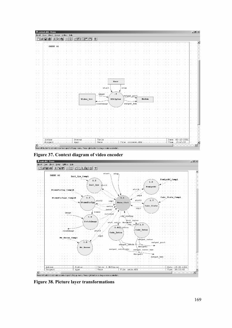
169
Figure 37. Context diagram of video encoder
Figure 38. Picture layer transformations

170
Figure 39. MB layer transformations
Figure 40. MB Layer transformation for the intra coding one coding scheme
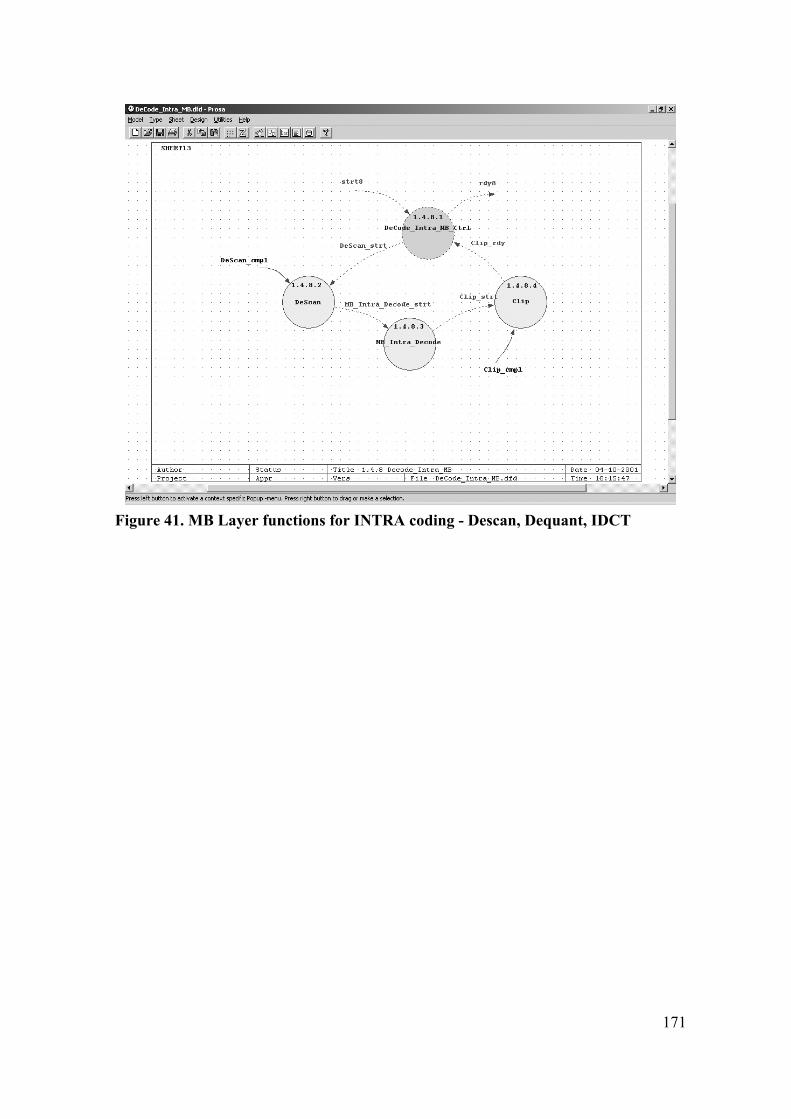
171
Figure 41. MB Layer functions for INTRA coding - Descan, Dequant, IDCT

172
Figure 42. H263 encoder reachability graph
173
7.2 Cost Estimation
Cost estimates are needed for modeling the problem setting and solving the
mapping and scheduling problem. At the early stages of design approximate estimates
are used. It is true that accurate costs estimates can be obtained also at the early stages
of design. This however requires that the tentative designs be worked out in quite some
detail, which is a costly exercise. Furthermore, the estimates obtained are very detailed
and implementation specific; they can often not be reused anymore. The assessment of
a larger number of designs using approximations of the costs that are computed
relatively fast is therefore preferred. The use of costs estimates does not mean that the
mapping and scheduling decision is straightforward; many unknowns exist and have to
be dealt with.
Whereas the information conveyed by accurate costs estimates is clear,
approximate estimates only give ballpark numbers. It is up to the system architect to
assess and interpret these numbers. It is not sufficient to only render the numbers. It is
as important that the method used to obtain the numbers is not a black box. This way
the system architect gains a better understanding of how to interpret the numbers.
Estimates for the design cost parameter of interest can often not be obtained in a
direct manner and proxy attributes are deployed. In the early stages of design it is
impossible to express criteria in monetary units. Proxy attributes do not measure the
cost parameter per se, but are correlated with it. Proxy attributes that have good
correlation with the design quality need therefore to be identified and specified.
Approximate costs estimates are based on an abstract cost model. The abstract
models for the system behavior and target architecture determine the structure of the
cost model. Attaching cost estimates to the structural components completes the cost
model. In order to develop the cost model, one needs to identify those aspects that
contribute to the costs. A selection then needs to be made of aspects that are included
in the model, or are omitted.
In this thesis, proxy attributes are used instead of spending much effort in obtaining
accurate estimates. Also, only the approximate system behavior of the system is
considered. Another simplifying assumption is the use of system runs or uses cases to
174
represent the system behavior. System runs are taken as starting point for making the
mapping and scheduling decision.
7.3 Cost Estimation of Data Transformation
SA/RT models involve data and control transformations. They contain the
algorithms respectively specify the way transformations cooperate. Because cost
estimates are difficult and costly to obtain, estimates for only the most significant
transformations are considered. Data transformations that require most of the
computations and transfer large amount of data, account for most of the costs. These
transformations need to be identified and their costs need to be estimated. Control and
other data transformations are taken into account as far as they determine the control
and data-flows; their computations are however not taken into account directly, but for
example as an overhead percentage.
In SA/RT models, data transformations are specified as pseudo-code. The design of
a system typically does not completely start from scratch. Embedded system
applications involve a number of algorithms that cooperate and need to be integrated.
These individual algorithms have mostly been studied in earlier projects or are
described in literature. The assumption that the functionality of the pseudo-code is
known to a certain extent can be made.
In this thesis, pseudo-code is used to obtain cost estimates for the data
transformation. It is assumed that the pseudo-code has been worked out to a level of
detail at which the inner loops that contain most of the computations are specified to
some extent. Typically the source code of these inner loops includes a number of basic
blocks with a simple flow of control. A basic block is a sequence of consecutive
statements that does not include instructions for branches or for halting, which makes
its behavior predictable.
In order to estimate the execution time of a basic block, a three-address instruction
code representation is generated. Three-address instructions have the general form z =
x oper y, where oper stands for any operator, such as arithmetic or logical operators,
and x,y,z are labels to data. The three-address instruction code is an intermediate
representation used in compilers. The back-end compiler assigns the actual machine
code instructions, memory locations and registers to the three address instructions.

175
Processors Cores - For processor core based architectures, the assumption is made
that there is a correlation between the number of operations in the three-address
instruction code for a basic block, and its execution time. Based on the application at
hand and components of the system architecture deployed, assumptions are made
about the way the obtained measures relate to the actual measure of interest. For
ballpark numbers these relations are limited to simple linear functions. The system
architect’s experience comes into play when making these assumptions. Assumptions
are often made tentatively and refined during the course of design (for example,
adjusting cache miss rates, memory waits etc).
Application Specific IC - For data-flow architectures with a data-path, a correlation
between the number of steps in the scheduling solution of the three-address instruction
code, and the basic block execution time is assumed. The data path architecture
includes a number of resources and registers that are allocated to operations each step
in the schedule. The scheduling solution is obtained using a heuristic algorithm that is
based on the list-scheduling algorithm. The scheduling algorithm used also takes the
use of registers into account.
7.4 Cost Estimation Method for Data Paths
The basic blocks in the inner loop can be represented as data-flow graphs. The
nodes represent operations and the (labeled) data operands; the edges represent the
flow of the control and the data, which entails the precedence relations between the
operations and operands.
Let ( ),G V E= be the graph representation of the three-address instruction code to
be scheduled, where the set V O D= ∪ contains the three-address code operations (O )
and the labeled data operands ( D ). The set E contains the graph edges. The set
{ }1, , nFU fu fu= … contains the functional units that make up the data-path. The
function ( ):u O FU→ P defines the set of functional units that can be used for an
operation. The set { }1, #, regR r r= … contains the registers in the data-path.
For the design case in this example, it is assumed that all operations require one
cycle, and that the register-bank is uniform. That is, the functional unit can access and
the operands can be stored in any registers. The following algorithm computes an

176
estimate for the number of cycles needed to execute an inner-loop. It is based on the
list-scheduling algorithm.
At every scheduling step s, a set of candidates for scheduling is determined. The
set contains the operations that can be invoked at step s. Candidate operations are only
selected and assigned to step s, if their requests for registers in combination the
existing ones can be met. Let LiveRegs denotes the set of operands that need to be
buffered in registers at scheduling step s.
At every scheduling step, candidate operations are selected from the operation
nodes in data-flow graph G that have not been scheduled yet. Let the data-flow graph
GOpen represents the sub-graph of G that has not been scheduled yet at scheduling
step s. Each unit fu FU∈ is allocated to an operation in the candidate set. The
operations selected form the candidate set CandidateSet. Let o be an operation node in
G, and is a candidate if the following properties hold.
• The functional unit fu checked matches the operator o that is ( )fu U o∈ .
• The nodes preceding operation o have in-degree zero. Nodes preceding
operation nodes are operands. If the operand nodes have in-degree zero, then
all its predecessors have been scheduled; the operand node is then ready to be
scheduled.
• There is sufficient space in the register-bank to store new input operands and
existing data operands. The number of live register plus the number of source
operands of operations in the candidate set should be less than the size of the
register bank..
( )# #LiveReg CandidateSet regs•∪ ≤ (7.1)
• Also, there should be sufficient space in the register-bank to store the results
and data operands that wait for their operations to take place. These operands
include operands that remain alive, since their target operator is not in the
candidate set ( ( )11sL + ). Or, the operand operator is in the candidate set; the
operand has however multiple targets and has pending operations ( ( )12sL + ). The
data operand is new in the set of live registers ( ( )13sL + ).
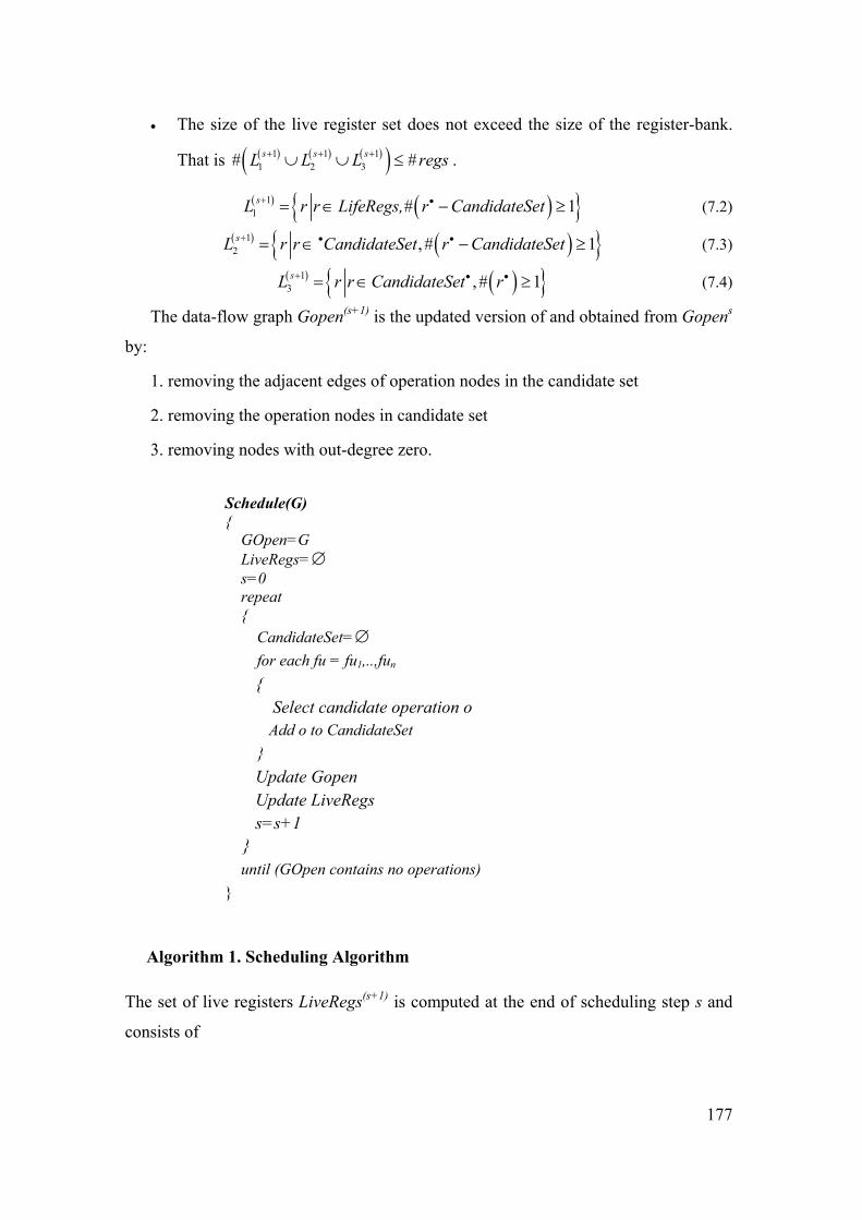
177
Schedule(G) { GOpen=G LiveRegs= ∅ s=0 repeat { CandidateSet=∅ for each fu = fu1,..,fun { Select candidate operation o Add o to CandidateSet } Update Gopen Update LiveRegs s=s+1 } until (GOpen contains no operations) }
• The size of the live register set does not exceed the size of the register-bank.
That is ( ) ( ) ( )( )1 1 11 2 3# #s s sL L L regs+ + +∪ ∪ ≤ .
( ) ( ){ }11 # 1sL r r LifeRegs, r CandidateSet+ •= ∈ − ≥ (7.2)
( ) ( ){ }12 , # 1sL r r CandidateSet r CandidateSet+ • •= ∈ − ≥ (7.3)
( ) ( ){ }13 , # 1sL r r CandidateSet r+ • •= ∈ ≥ (7.4)
The data-flow graph Gopen(s+1) is the updated version of and obtained from Gopens
by:
1. removing the adjacent edges of operation nodes in the candidate set
2. removing the operation nodes in candidate set
3. removing nodes with out-degree zero.
The set of live registers LiveRegs(s+1) is computed at the end of scheduling step s and
consists of
Algorithm 1. Scheduling Algorithm

178
1. Data operands that are in LiveRegss and have out-degree larger than zero in
Gopen(s+1), that is, there are operations pending for which they serve as input.
2. Data operands that are succeeding the operations in the candidate set, and have
operations pending for which they serve as input.
The number of steps represents the number of cycles it takes to execute the inner
loop basic block. Based on the inner loop count estimate and the estimates for the basic
blocks, an estimate for the transformation execution time is obtained.
For processor core based architectures, there is reasonably a correlation between
the number of instructions in the basic blocks, and the transformation instruction code
size. The effects of instruction caches can be taken into account by notions such as
cache miss rate. In this example, the instruction code is loaded manually into the local
kernel memory. The number of three-address instructions is used as proxy attribute to
represent the costs of loading the instruction node in the processor local memory.
There is reasonably also a correlation between the size of the data used in the source
code and the costs of data transfers.
The execution time estimation for the basic block example below is discussed. For
a processor based kernel, or a kernel with data-path two different versions of the three-
address instruction code is used for cost estimation.
For processor core based architectures, the assumption is made that instructions
cannot directly use the contents of memory locations as operands since the processor
involved in relatively simple. The address of, or the data in memory locations needs
first to be loaded in a register before they can be used as operands for instructions.
Similarly, the use of a variable as the destination of a three-address instruction requires
a store operation. Figure 43 and Figure 44 depict the two different data-flow graph
versions for the processor core based and data-flow architecture with data path,
respectively.
• float a,b,c,d • B1: • a=b*2+c*30; • d=(a+b)+(c+5);
Algorithm 2. Basic block example
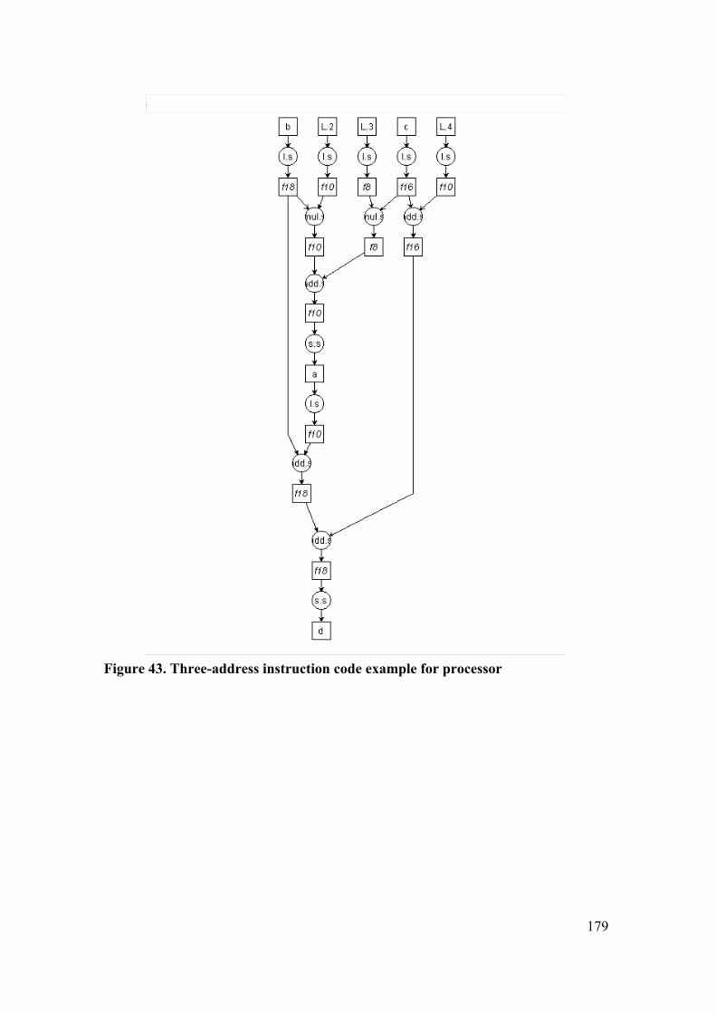
179
Figure 43. Three-address instruction code example for processor
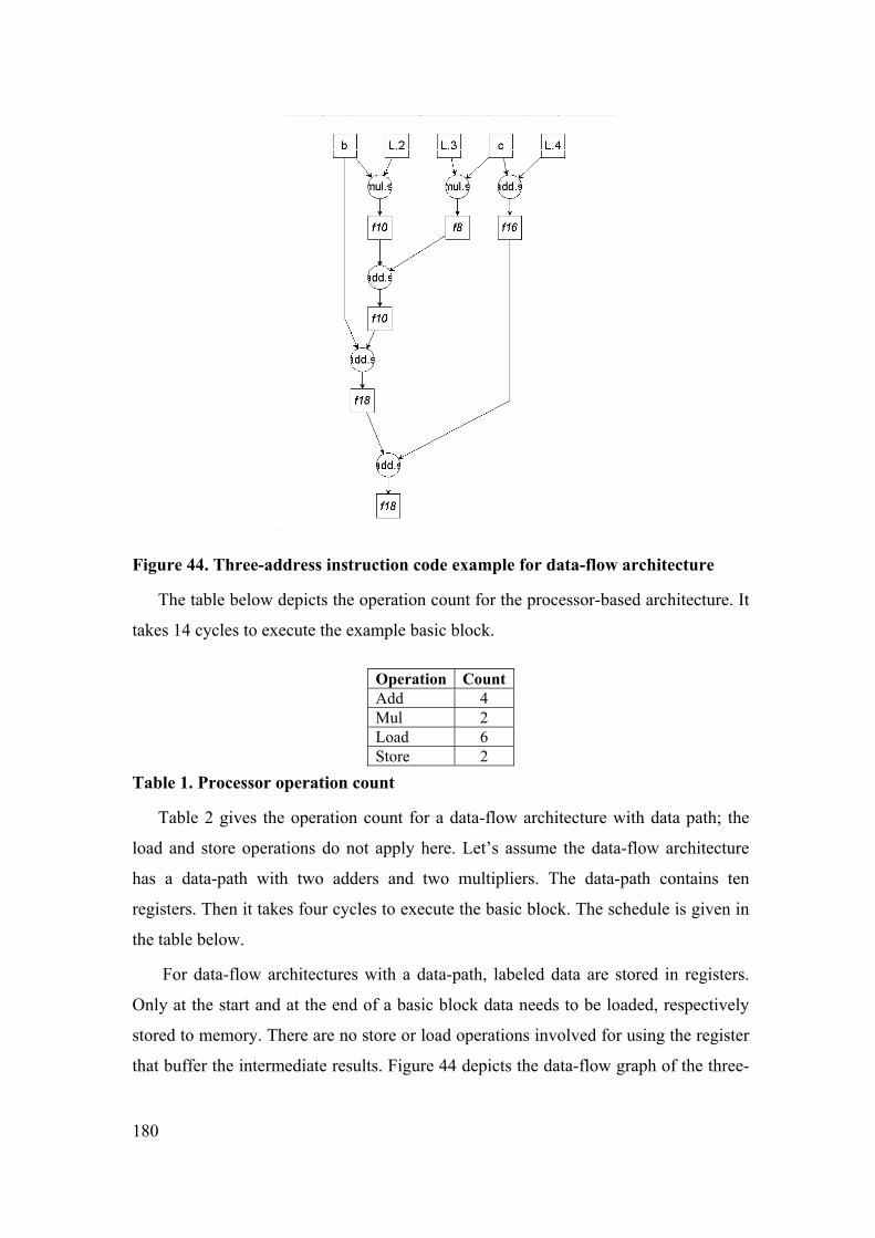
180
Figure 44. Three-address instruction code example for data-flow architecture
The table below depicts the operation count for the processor-based architecture. It
takes 14 cycles to execute the example basic block.
Operation CountAdd 4 Mul 2 Load 6 Store 2
Table 1. Processor operation count
Table 2 gives the operation count for a data-flow architecture with data path; the
load and store operations do not apply here. Let’s assume the data-flow architecture
has a data-path with two adders and two multipliers. The data-path contains ten
registers. Then it takes four cycles to execute the basic block. The schedule is given in
the table below.
For data-flow architectures with a data-path, labeled data are stored in registers.
Only at the start and at the end of a basic block data needs to be loaded, respectively
stored to memory. There are no store or load operations involved for using the register
that buffer the intermediate results. Figure 44 depicts the data-flow graph of the three-
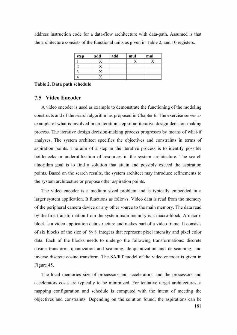
181
address instruction code for a data-flow architecture with data-path. Assumed is that
the architecture consists of the functional units as given in Table 2, and 10 registers.
step add add mul mul 1 X X X 2 X 3 X 4 X
Table 2. Data path schedule
7.5 Video Encoder
A video encoder is used as example to demonstrate the functioning of the modeling
constructs and of the search algorithm as proposed in Chapter 6. The exercise serves as
example of what is involved in an iteration step of an iterative design decision-making
process. The iterative design decision-making process progresses by means of what-if
analyses. The system architect specifies the objectives and constraints in terms of
aspiration points. The aim of a step in the iterative process is to identify possible
bottlenecks or underutilization of resources in the system architecture. The search
algorithm goal is to find a solution that attain and possibly exceed the aspiration
points. Based on the search results, the system architect may introduce refinements to
the system architecture or propose other aspiration points.
The video encoder is a medium sized problem and is typically embedded in a
larger system application. It functions as follows. Video data is read from the memory
of the peripheral camera device or any other source to the main memory. The data read
by the first transformation from the system main memory is a macro-block. A macro-
block is a video application data structure and makes part of a video frame. It consists
of six blocks of the size of 8 8× integers that represent pixel intensity and pixel color
data. Each of the blocks needs to undergo the following transformations: discrete
cosine transform, quantization and scanning, de-quantization and de-scanning, and
inverse discrete cosine transform. The SA/RT model of the video encoder is given in
Figure 45.
The local memories size of processors and accelerators, and the processors and
accelerators costs are typically to be minimized. For tentative target architectures, a
mapping configuration and schedule is computed with the intent of meeting the
objectives and constraints. Depending on the solution found, the aspirations can be

182
raised, or if necessary lowered. Modifications to the target architecture involve, for
example, changes in some of the capacities of the components, or
introducing/removing complete components; proposals for modifications come
entirely from the system architect.
DCT QNT/SCN
DQNT/DSCN IDCT
block block block
macro-block
compresseddata
1..6
Figure 45. SA/RT model of video encoder
Finding a transformation-to-architecture mapping is not straightforward since
resources are limited and the use of a resource by one transformation is strongly
related to the use of resources by other transformations. For example, the instruction
code for transformations is preferably stored in the local memory for fast access. This
prevents the processor from being stalled. In case there is no separate instruction and
data memory, then local memory space is also needed for buffering the data blocks
that are in transit between transformation runs. The assumption is made that the
designer has full control over the data present in the local memory. Because multiple
data sets needs to be present in the local memory at the same time, the loading and
storing of data needs to be planned which becomes the designer’s responsibility.
Another decision, which involves interrelated aspects, is the mapping of
functionality to the accelerator. This not necessarily speed up the execution of the
algorithm, since data need to be transferred to, and read back to the processor local
memory. Here increase of local memory space, possibly decreases the amount of
resources needed for the accelerator.
The operation counts for the transformations of the video encoder are given in the
tables below. Each of the basic blocks is executed 8 times per block input sample. The
abstract model of the data-path consists of one shifter, two adders and two multipliers
for integer operands, two adders and two multipliers for floating-point operands, and
183
thirty registers. The table below also gives the execution time for the transformation
when implemented using a simple processor core based architecture, or data-flow
architecture with the data-path described above. The table also gives the blocks and
stores associated with the transformations.
Blocks involve data that is shared and used by multiple transformations runs. In
this example, instruction code is loaded manually from the main memory, or ROM for
example, to the local memory and needs to be planned. Instruction code for the
transformations can be modeled as blocks. Stores represent the SA/RT model stores.
The proxy measures for blocks and stores are given in the table below. It is assumed
that there is a correlation between the number of three-address instruction code for a
transformation, the instruction code size and, in this example, the time needed to load
the instruction code. For stores, it is assumed that there is a correlation between the
number of integers sent and the time it takes to load or store the data.
In this example, the assumption is made that in case the instruction code needs to
be loaded just before the start of its transformation run because it is unavailable, then it
causes an additional delay to the transformation run. The instruction code size can
hereby used as a measure. Furthermore, it is assumed that it takes a cycle to load and
store an integer.
The cost estimates are used to “populate” the optimization model as specified in
the previous chapter. The search process is implemented as a genetic algorithm. Five
types of objectives are considered in the genetic algorithm:
1. The makespan of the system
2. The maximal amount of memory used in the processor
3. The maximal amount of used in the accelerator
4. The amount of data loaded into and stored from the local processor memory
5. The amount of data loaded into and stored from the local accelerator memory
Additionally the average memory use over time can be used as criterion to further
discern between almost similar alternatives in the search process.
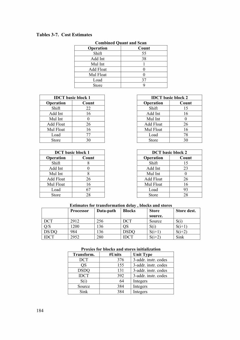
184
Tables 3-7. Cost Estimates
Combined Quant and Scan Operation Count
Shift 55 Add Int 38 Mul Int 1
Add Float 0 Mul Float 0
Load 37 Store 9
IDCT basic block 1 IDCT basic block 2
Operation Count Operation Count Shift 22 Shift 15
Add Int 16 Add Int 16 Mul Int 0 Mul Int 0
Add Float 26 Add Float 26 Mul Float 16 Mul Float 16
Load 77 Load 78 Store 30 Store 30
DCT basic block 1 DCT basic block 2
Operation Count Operation Count Shift 8 Shift 15
Add Int 0 Add Int 23 Mul Int 8 Mul Int 0
Add Float 26 Add Float 26 Mul Float 16 Mul Float 16
Load 67 Load 93 Store 28 Store 28
Estimates for transformation delay , blocks and stores
Processor Data-path Blocks Store source.
Store dest.
DCT 2912 256 DCT Source S(i) Q/S 1200 136 QS S(i) S(i+1) DS/DQ 984 136 DSDQ S(i+1) S(i+2) IDCT 2952 280 IDCT S(i+2) Sink
Proxies for blocks and stores initialization Transform. #Units Unit Type
DCT 376 3-addr. instr. codes QS 155 3-addr. instr. codes
DSDQ 131 3-addr. instr. codes IDCT 392 3-addr. instr. codes S(i) 64 Integers
Source 384 Integers Sink 384 Integers

185
The system architect’s preferences are given as aspiration points, and solutions are
searched that meet and possibly exceed the aspiration points. As discussed in 3.4.2
solutions that meet the aspiration are assigned the utility 0.9 with regard to the
criterion. Figure 46 shows the achievement functions for objectives: makespan, and
local processor and accelerator memory use.
To demonstrate the proper functioning of the search algorithm, the search for a
mapping and scheduling solution that has a makespan of less than 1500 operation
cycles, and local memory capacity for the processor and accelerator of less than 90
units (1 unit = 8 integers) is performed, The transformation runs that make up the
encoder should be completed within 1500 cycles, and there should be at all times less
than 90 memory units (1 unit = 8 integers) allocated to blocks and stores in local
memory of the processor and accelerator..
The search starts with the generation of population of 200 individuals at random.
For the aspiration points specified, none of the individuals meet the requirements; the
aspiration points seems to be chosen properly for exploring the boundaries of what is
feasible for the encoder, and which tradeoffs can be made between the makespan and
amount of local memory in the processor and accelerator.
makespan memory useprocessor/accelerator
utility utility
1500 200010005000
1.00.9
0.6
0.4
0.2
0.090 12060300
1.00.9
0.6
0.4
0.2
0.0
Figure 46. Makespan and processor/accelerator memory use achievement funct.
Figure 50 shows the makespan, and memory use of individuals in the population at
iteration 1, 41, 81 and 121. As shown in the figure, the overall quality of the
population improves steadily, and the aspiration point is approached. Also the diversity
in the population is maintained, the solutions do not clutter towards only a small
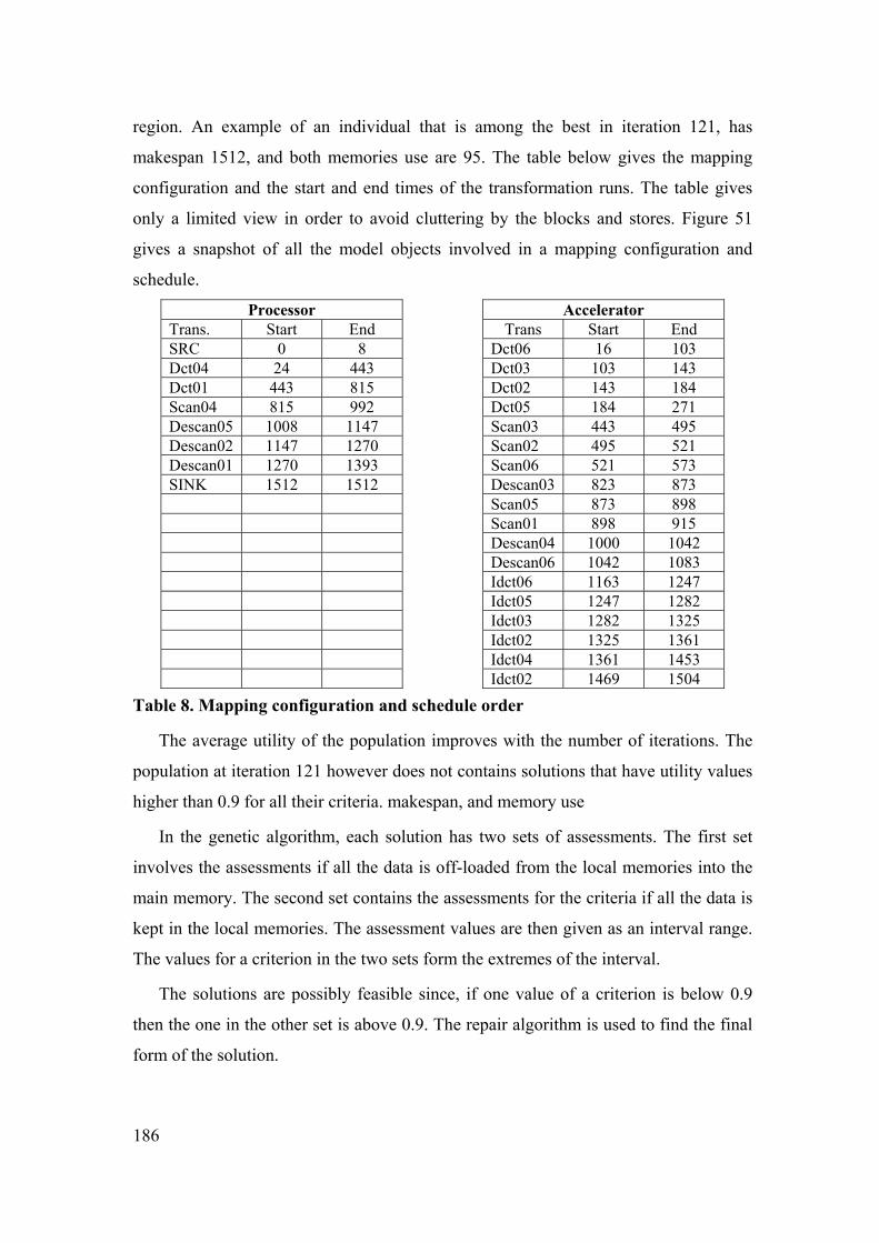
186
region. An example of an individual that is among the best in iteration 121, has
makespan 1512, and both memories use are 95. The table below gives the mapping
configuration and the start and end times of the transformation runs. The table gives
only a limited view in order to avoid cluttering by the blocks and stores. Figure 51
gives a snapshot of all the model objects involved in a mapping configuration and
schedule.
Processor Accelerator Trans. Start End Trans Start End SRC 0 8 Dct06 16 103 Dct04 24 443 Dct03 103 143 Dct01 443 815 Dct02 143 184 Scan04 815 992 Dct05 184 271 Descan05 1008 1147 Scan03 443 495 Descan02 1147 1270 Scan02 495 521 Descan01 1270 1393 Scan06 521 573 SINK 1512 1512 Descan03 823 873 Scan05 873 898 Scan01 898 915 Descan04 1000 1042 Descan06 1042 1083 Idct06 1163 1247 Idct05 1247 1282 Idct03 1282 1325 Idct02 1325 1361 Idct04 1361 1453 Idct02 1469 1504
Table 8. Mapping configuration and schedule order
The average utility of the population improves with the number of iterations. The
population at iteration 121 however does not contains solutions that have utility values
higher than 0.9 for all their criteria. makespan, and memory use
In the genetic algorithm, each solution has two sets of assessments. The first set
involves the assessments if all the data is off-loaded from the local memories into the
main memory. The second set contains the assessments for the criteria if all the data is
kept in the local memories. The assessment values are then given as an interval range.
The values for a criterion in the two sets form the extremes of the interval.
The solutions are possibly feasible since, if one value of a criterion is below 0.9
then the one in the other set is above 0.9. The repair algorithm is used to find the final
form of the solution.

187
The aspiration specified seems to be a Pareto optimal point. Improvement of one of
the objectives leads to deterioration of another. This sort of information drives the
what-if analyses.
The functioning of the selection operator is critical for the performance of genetic
algorithms. On one hand there is the need to propagate only high potential individuals
to the next generation. On the other hand, the population should be diverse enough in
order not to overlook promising alternatives. If no measures are undertaken to
maintain diversity or to prevent a biased selection process, then the search tends to
wander off into a limited region of the decision and/or objective space, which not
necessarily contain the optimal solution. For this reason, firstly, the search is equipped
with MCDM methods and techniques in order to better discern between the
alternatives and this way prevent making selections that are unnecessary crude and
cannot be justified. Secondly, additional measure can be adopted which makes the
differences between solutions that are rather similar to stand out more. Thirdly,
measures, such as crowding distances, which give an indication of the individual’s
contribution to the population diversity, can be used to distinguish between
alternatives. In this thesis, all three measure are used, which seems to be sufficient for
a properly function selection operator with which the right balance between diversity
and search convergence can be made.

188
. Figure 47. Search progress for makespan and local processor memory
Figure 48. Search progress for makespan and local accelerator memory

189
Figure 49. Search progress for local memories in processor and accelerator
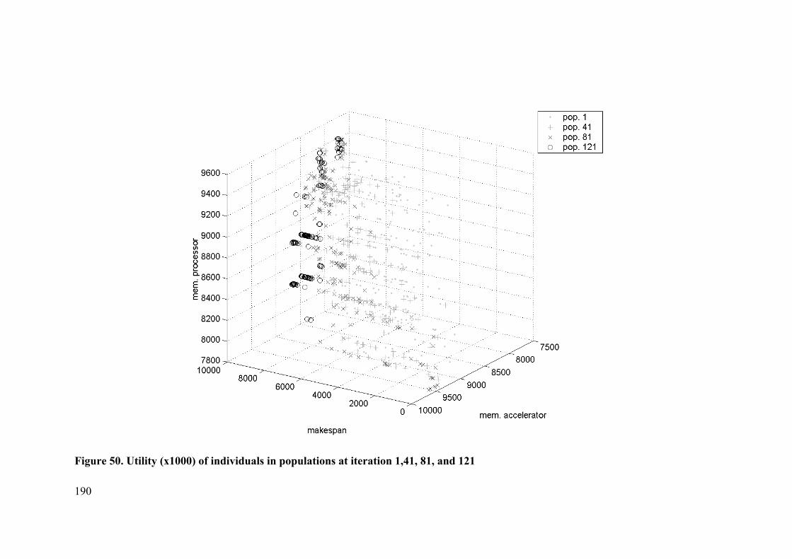
190
Figure 50. Utility (x1000) of individuals in populations at iteration 1,41, 81, and 121
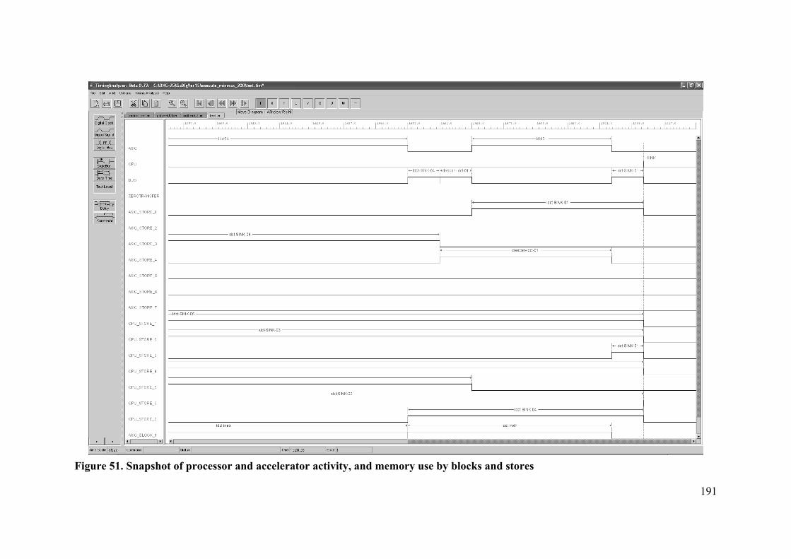
191
Figure 51. Snapshot of processor and accelerator activity, and memory use by blocks and stores

193
Chapter 8. Conclusions
There is a need to exploit the opportunities silicon technology is providing in an
effective and efficient manner. As the size and complexity of real-time embedded
systems increase, the specification and design of the overall system architecture become
not less, but often even more significant issues than the choice of particular algorithms,
data structures and their particular implementation. During system-level design of real-
time embedded systems, one should therefore adhere to sound principles and concepts
apt for design-in-the large, and use only a limited set of suitable techniques and
mechanisms.
In the architecture exploration phase in system design, the generation of system
architectures basically involves the three sub-problems of allocation, mapping and
scheduling. In order to be able to make the right system architecture selection, the
feasibility of candidate functional behavior - hardware architecture pairs need to be
predicted.
The subject of the research reported in this thesis is the semi-automatic selection of
system architectures for application-specific real-time embedded systems using multi-
criteria decision-making aids. The design decision-making is in particular related to the
mapping and scheduling of the system behavior (network of the system processes) on the
system structure (network of the system structural modules) in the light of the system
parametric constraints and objectives.
The main contribution is the development of a method to predict the feasibility of
specific hardware architecture – requirements model pairs. The method facilitates in:
• the creation of a model, which is based on the requirements models, and which
characterizes the functional behavior, facilitates behavioral analysis, mapping and
scheduling, and properly expose the impact of system architecture decisions.
194
• the construction of the modeling constructs that defines the decision space for the
mapping and scheduling problem
• the construction of the heuristic search that is organized as a genetic algorithm for
predicting the feasibility of the candidate functional behavior – hardware
architecture pairs.
The decision model integrates many kinds of different data. It requires models of
processes, definition of relationships between tasks and resources, definition of
objectives and performance measures and the underlying data and decision variables and
algorithms that tie them all together. Usually, computations are considered to be the main
contributor to implementation costs. As architectures become distributed, data transfers
become a major cost component. Data transfer typically translates into data movements
between peripheral and processor memories. For this reason the memory organization in
a system becomes more important. Modeling constructs are proposed that model the
costs and impact memories have on the system performance.
The search for a satisfactory solution is implemented as a parallel search that works
with populations of solutions considering a number of solutions in parallel. The genetic
algorithm developed assumes a random population with a limited number of individuals
at the beginning. Crossover and mutation operators have been defined that make
combinations respectively create variants of the most promising individuals in the
population.
The search process involves ranking and selection problems. MCDM concepts and
methods are considered to be beneficial and have been deployed. The problem of
constructing the decision model is the same in decision theory and system design. The
preferences model is not an objective reality and is based on information elicited from
the system architect. For this reason the preferences model should not be based on strong
assumptions that are difficult to justify, let alone verify. Instead, preferences models are
constructed that require limited trade-off information from the system architect and that
can handle imprecise assessments. MCDM methods and techniques have been adapted to
the system design problem setting. They are applied in the frame of a heuristic search for
solutions based on genetic algorithms.
The method is semi-automatic, that is, the system architect performs what if analyses,
by first generating candidate hardware architectures, analyzing the mapping and

195
scheduling results, and generating proposals for refinements. The mapping and
scheduling is performed automatically by heuristic search and involves the making of
numerous trade-off decisions that meet the system parametric constraints and objectives.
During the heuristic search some promising instantiations of the system architecture are
proposed, estimated and selected for further propagation. Identifying potential
bottlenecks and architecture improvements however remains the task of the system
architect.
The development of the method resulted in contributions in the following areas.
Organization of Problem Solving Process - In this thesis, a specific and original
realization of the quality-driven design paradigm as proposed by Jóźwiak [79] has been
developed for solving the mapping and scheduling problem of requirements model –
hardware architecture pairs for architecture exploration in the system-level design phase.
It is argued that the system design problems need to be modeled first due to their
complexity, diversity, poor structure and dynamic character; the model is only a
subjective representation of reality that evolves along the course of its development. The
evolutionary design process is implemented by appropriately modeling the design
problems, using the models and search tools equipped with multi-criteria decision-
making aids to find, estimate and select some promising alternative solutions.
Exposure of the On-chip Memory Use and Communication - Distinct from other
system architecture synthesis approaches, the mapping and scheduling of memory use by
processes and communication actions is integrated in the mapping and schedule problem.
Communication actions are usually modeled to only consume time, and bus capacity.
Memories and memory ports are hardware primitives, and just like other primitives they
can be assigned and scheduled for some time to process, communication actions, or data
objects. The mapping configuration and precedence and conflict relations between the
elements determine which memory is to be assigned to what functional element and for
how long. Novel and original modeling constructs have been developed that approximate
the use patterns of these memories.
Execution Rules, Translation Method, Traces Extraction for SA/RT Models – The
execution rules of SA/RT is semi-formal. New and original execution rules have been
developed which formalizes the behavior of SA/RT. Also, a novel construction method

196
has been developed with which a SA/RT model can be translated into and represented as
a set of communication processes that use CSP-like communication and synchronization
actions; the construction method translates SA/RT models into elementary net systems.
Difficulty hereby is that SA/RT models are in origin a mixed synchronous/asynchronous
models; primitive data and event flows in the SA/RT need to be grouped and cast onto
their asynchronous counterpart. Execution rules are a pre-requisite to extract traces (with
branches) from the SA/RT model based on some use case. These traces form a
representation of the functional behavior of the SA/RT model and serves as building
block for the mapping and schedule decision model. Various abstract behavior models
that enable static timing and resource analysis based on traces for SA/RT models,
together with timing and resource usage estimation procedures have been developed in
this thesis. The estimation procedures make use of an abstraction of the hardware
resource characteristics.
Heuristics Search Method for Mapping and Scheduling – A new deployment
scheme for GA and CSP for optimization has been developed. The scheme makes use of
sensitivity information; the decision variables for which the solution has a high
sensitivity are resolved first. In a second (post-processing) stage the remaining decision
variables that are possibly difficult to solve using GA due to the constraints involved, are
set. Also, the non-dominated sorting method has been enhanced, in order to better
discern the alternatives mutual ranking.
Design cases have been worked out to analyze and test all the parts; they have been
checked together. A behavioral analysis and search and optimization exercise for a
medium sized system has been carried out. The experimental research confirms the
adequacy of the proposed approach.
A method for modeling application-specific real-time embedded systems for the
semi-automatic design decision-making related to the system architecture exploration
phase in system design has been proposed and deployed for experimental purposes. A
specific realization of the quality-driven design decision-making process for the mapping
and scheduling problem in system design has been developed. Design issues that are
increasingly important as silicon technology advances are taken into consideration. For
this reason, this research substantially contributes to creation of the adequate

197
methodological base for development of complex microelectronic-based systems,
including SoCs.

198
199
REFERENCES
[1] G. Arnout, “SystemC Standard”, Proceedings of the ASP-DAC 2000, pp. 573-77,
2000.
[2] Peter J. Ashenden, The Designer's Guide for VHDL, Morgan Kaufman}, 1996.
[3] Audsley, N.C., et al. "Fixed Priority Pre-Emptive Scheduling: An Historical
Perspective." Real Time Systems 8, 2-3. (March-May 1995): 173-98.
[4] M. Awed, J. Ukulele, and J. Ziegler, Object-Oriented Technology for Real Time
Systems: A Practical Approach Using OMT and Fusion, Prentice Hall, 1996.
[5] Th. Back, U. Hummel and H.-P. Schaefer, “Evolutionary Computation:
Comments on the History and Current State”, IEEE Trans. on Evolutionary
Computation, vol. 1, no. 1, April 1997.
[6] Eds. T. Back et.al., “Evolutionary Computation 1, Basic Algorithms and
Operators”, IOP Publishing Ltd., 2000.
[7] Eds. T. Back et.al., “Evolutionary Computation 2, Advanced Algorithms and
Operators”, IOP Publishing Ltd., 2000.
[8] F. Balarin et.al., Hardware-Software Co-Design of Embedded Systems: The Polis
Approach, Kluwer Academic, 1997.
[9] F. Balarin et.al., “Metropolis: An Integrated Electronic System Design
Environment”, IEEE Computer, vol. 36, nr. 4, April 2003.
[10] Balboni et.al., “Co-Synthesis and Co-Simulation of Control-Dominated
Embedded Systems”, Design Automation of Embedded Systems, vol. 1, no. 3,
pp. 257-289, July 1996.
[11] Luciano Baresi, Mauro Pezzè, “Toward formalizing structured analysis”, ACM
Transactions on Software Engineering and Methodology (TOSEM), Volume 7
Issue 1, January 1998.
[12] M. Bauer et.al., “A method for accelerating test environments”, in Proceedings.
25th EUROMICRO Conference, vol. 1, pp. 477-80, 1999.
200
[13] Bender, “Design of an Optimal Loosely Coupled Heterogeneous Multiprocessor
System”, in Proceedings of The European Design & Test Conference, pp. 275-
281, 1996.
[14] J.A. Bergstra and J.W. Klop, “Algebra of communicating processes with
abstraction”, Theoretical Computer Science, vol. 37, nr. 1, pp. 77-121, 1985.
[15] G. Berry and G. Gonthier, “The Esterel Synchronous Programming Language:
Design, Semantics, Implementation”, Science of Computer Programming, vol.
19, no. 2, pp. 87-152, 1992.
[16] F. Boussinot and R. de Simone, “The Esterel Language”, Proceedings of the
IEEE, Special Issue: Another Look at Real-time Programming, vol. 79, no. 9, pp.
1293-1304, Sept. 1991.
[17] J. Buck et.al., “Ptomely, A Framework for Simulating and Prototyping
Heterogeneous Systems”, Int. J. of Computer Simulation, Jan. 1995.
[18] J. Buck and R. Vaidyanathan, “Heterogeneous modeling and simulation of
embedded systems in El Greco”, in Proceedings of 8th CODES, pp. 142-46,
2000.
[19] J.P. Calvez, “A Co-Design Case Study with the MCSE Methodology”, Design
Automation of Embedded Systems, vol. 1, no. 3, pp. 183-212, July 1996.
[20] R. Camposano and J. Wildberg, “Embedded System Design”, Design Automation
for Embedded Systems, vol. 1, pp. 5-50, Kluwer, 1996.
[21] W.O. Cesário, G.Nicolescu, L. Gauthier, D. Lyonnard, and A.A. Jerraya, “Colif:
A Design Representation for Application-Specific Multiprocessor SOCs”, IEEE
Design and Test, Sept.-Oct. 2001.
[22] B. Charron-Bost, F. Mattern and G. Tel, “Synchronous, Asynchronous, and
Causally Ordered Communication”, Distributed Computing , vol. 9 nr. 4, pp.
173-191, 1996
[23] S.-J. Chen and C.-L. Hwang, “Fuzzy Multiple Attribute Decision-Making,
Methods and Applications”, Springer Verlag, 1992.
[24] M. Chiodo et.al., “A Formal Specification Model for Hardware-Software Co-
design”, Proc. of the Int. Workshop on Hardware-Software Co-design 1993.
201
[25] E.M. Clarke et.al., “Automatic Verification of Finite State Concurrent Systems
Using Temporal Logic Specifications”, ACM Transactions on Programming
Languages and System, vol. 8, nr. 2, 1986, pp. 244-263.
[26] R. Cleaveland et.al., “Priority in Process Algebras”, NASA Tech. Rep. 99-3,
1999.
[27] G. Cote et.al., H.263+: "Video Coding at Low Bit Rates", IEEE Trans. On
Circuits and Systems for Video Technology, Vol. 8, Nr. 7 Nov. 1998.
[28] B.G.W. Craenen, A.E. Eiben and E. Marchiori, “How to Handle Constraints with
Evolutionary Algorithms”.
[29] P. Darondeau and P. Degano., “Event Structures, Causal Trees, and
Refinements”, in Proc. Mathematical Foundations of Computer Science 1990,
Czechoslovakia, August 1990, published in LNCS 452, Springer Verlag.
[30] Bharat P. Dave et.al., “COSYN: Hardware-Software Co-Synthesis of
Heterogeneous Distributed Embedded Systems”, IEEE Trans. On VLSI
Systems”, vol. 7, no. 1, March 1999.
[31] P. Bogetoft and P. Pruzan, “Planning with Multiple Criteria: Investigation,
Communication and Choice”, Copenhagen Business School Press, 1999.
[32] Kalyanmoy Deb, “Multi-Objective Optimization Using Evolutionary
Algorithms”, Wiley 2001.
[33] J.A. Debardelaben and V.K. Madisetti, “Hardware/software co-design for signal
processing systems. A survey and new results”, in Proceedings Asilomar ‘95, vol.
2, pp. 1316-20, 1995.
[34] G. DeMicheli, “Computer-Aided Hardware-Software Co-design”, IEEE Micro,
pp. 10-16, August 1994.
[35] G. DeMicheli and R.K. Gupta, Hardware/software co-design, Proceedings of the
IEEE , vol. 85, no. 3, pp. 349-65, March 1997.
[36] Dick, R.P. and Jha, N.K., “MOGAC: a multiobjective genetic algorithm for
hardware-software cosynthesis of distributed embedded systems”, IEEE Trans. of
Computer-Aided Design of Integrated Circuits and Systems, vol. 18, nr. 10, 1999.
[37] B.P. Douglass, Doing Hard Time: Developing Real-Time Systems with UML,
Objects, Frameworks and Patterns, Addison-Wesley, 1999.
202
[38] P. Eles, K. Kuchcinski, Z. Peng, P. Pop, and A. Doboli. Scheduling of conditional
process graphs for the synthesis of embedded systems. In Proc. Design,
Automation and Test in Europe - DATE, 1998.
[39] R. Ernst et.al., "Hardware/Software Co-Synthesis for Microcontrollers", IEEE
Design & Test Magazine, vol. 10, no. 4, pp. 64-75, December 1993.
[40] R. Ernst, “Co-design of Embedded Systems: Status and Trends”, IEEE Design &
Test of Computers, vol. 15, no. 2, pp. 45-54, 1998.
[41] R. Ernst, D. Ziegenbein, K. Richter, L. Thiele, and J. Teich. Hardware/Software
Codesign of Embedded Systems - The SPI Workbench. Proc. Int. Workshop on
VLSI, Orlando, U.S.A., 1999.
[42] Robert Esser, et.al. “Applying an Object-Oriented Petri Net Language to
Heterogeneous Systems Design”. In Proceedings of Petri Nets in System
Engineering, Hamburg, Germany, pp. 24-25, September 1997.
[43] D.G. Evans et.al., “A Systems Approach to Embedded Systems Development”, in
Embedded Microprocessor Systems, pp. 371-382, IOS Press, Amsterdam, 1996.
[44] M. Felder and M. Pezzè, “A formal design notation for real-time systems”, ACM
Transactions on Software Engineering and Methodology (TOSEM), Volume 11 ,
Issue 2, April 2002.
[45] D.D. Gajski and F. Vahid, “Specification and Design of Embedded Hardware-
Software”, IEEE design and Test of Computers, spring issue, pp. 53-67, 1995.
[46] D.D. Gajski et.al., “SpecSyn: an environment supporting the specify-explore-
refine paradigm for hardware/software system design”, IEEE Transactions on
Very Large Scale Integration (VLSI) Systems, vol. 6, no. 1, pp. 84-100, March
1998.
[47] D.D. Gajski, High-Level Synthesis : Introduction to Chip and System Design,
Kluwer Academic, 1992.
[48] C.H. Gebotys and M.I. Elmasry, Optimal VLSI Architectural Synthesis : Area,
Performance and Testability, Kluwer Academic, 1992.
[49] Richard Goering, “Giga-center redefines chip design for new millennium”, EE
Times, march 1st 2000.
[50] F. Glover and M. Laguna, Tabu Search, Kluwer Academic Publishers, 1997
203
[51] F. Glover and M. Laguna, Tabu Search, in Ed. C. Reeves, Modern Heuristic
Techniques for Combinatorial Problems, Kluwer Scientific Publications, 1993.
[52] J. Gong et.al., “Model Refinement for Hardware-Software Co-design”, in
Proceedings of The European Design & Test Conference, pp. 270-274, 1996.
[53] L. Guerra et.al., “Cycle and phase accurate DSP modeling and integration for
HW/SW co-verification”, in Prodeedings of 36th Design Automation Conference,
pp. 964-9, 1999.
[54] R.K. Gupta, C.N. Coelho and G. DeMicheli, “Program Implementation Schemes
for Hardware-Software Systems”, IEEE Computer, vol. 27, no. 1, January 1994.
[55] R.K. Gupta and G. DeMicheli, “Hardware-Software Cosynthesis for Digital
Systems”, IEEE Design and Test, vol. 10, no. 3, September 1993.
[56] R.K. Gupta and G. DeMicheli, “Constrained Software Generation for Hardware-
Software Systems”, Proc. of the Int. Workshop on Hardware-Software Codesign
1994.
[57] N. Halbwachs, Synchronous Programming of Reactive Systems, Kluwer
Academic Publ., 1993.
[58] D. Harel and A. Pneuli, “On the Development of Reactive Systems”, ACM 1985.
[59] David Harel, “StateCharts: a Visual Formalism for Complex Systems”, Science
of Computer Programming, vol. 8, no. 3, pp. 231-75, 1987.
[60] David Harel and Amnon Naamad, “The STATEMATE Semantics of
StateCharts”, ACM Trans. On Software Engineering and Methodology, vol. 5,
no. 4, pp. 293-333, Oct. 1996.
[61] G.R. Hellestrand, “The revolution in systems engineering”, IEEE Spectrum, vol.
36, no. 9, pp. 43-51, Sept. 1999.
[62] G.R. Hellestrand, “Designing system on a chip products using systems
engineering tools”, in Proceedings ISCAS '99, vol. 6, pp. 468-73, 1999.
[63] M. Henenessy, Algebraic Theory of Processes, The MIT Press, 1988.
[64] C.A.R. Hoare, Communicating Sequential Processes, Prentice-Hall, 1985.
[65] D. Hocevar et.al., “A Performance Simulation Approach for MPEG Audio/Video
Decoder Architectures, ACM Winter Simulation Conference.

204
[66] G. Holtzmann, “Design and Validation of Computer Protocols”, Prentice-Hall
1991.
[67] T. Hopes, “Hardware/software co-verification, an IP vendors viewpoint”, in
Proceedings ICCD '98, pp. 242-46, 1998.
[68] H. Hsieh, F. Balarin, L. Lavagno, A. Sangiovanni-Vincentelli, “Efficient methods
for embedded system design space exploration”, Proc. of the DAC, IEEE, 2000.
[69] Richard E. Howard, “The unwired world, the hard job of making it look easy”,
Bell Laboratories, 1998.
[70] S. H. Huang et.al, "A tree-based scheduling algorithm for control-dominated
circuits", Proc. of the 30th int. conf. on Design Automation, pp. 578 - 582,
IEEE/ACM 1993.
[71] C.-L. Hwang and A.S. Masud, “Multiple Objective Decision Making Methods
and Applications”, vol. 164 of Lecture Notes in Economics and Mathematical
Systems, Springer Verlag 1979.
[72] Insoft OY, Prosa Structed Analysis and Design Environment, User’s Manual,
1998.
[73] T.B. Ismail and A.A. Jerraya, “COSMOS: a co-design approach for
communicating systems”, in Proceedings of the 3rd Int. Workshop on
Hardware/Software Co-design, pp. 17-24, 1994.
[74] T.B: Ismail and A.A. Jerraya, “Synthesis Steps and Design Models for Co-
design”, IEEE Computer, pp. 44-52., Febr. 1995.
[75] ITU-T, “Video coding for low bit rate communication, H.263”, 02/98.
[76] M.A. Jackson, System Development, Prentic Hall 1983.
[77] P.P. Jain, “Cost-effective co-verification using RTL-accurate C models”, in
Proceedings ISCAS '99, vol. 6, pp. 460-63, 1999.
[78] L. Józwiak: Subjective Aspects of Quality in the Design of Complex
Hardware/Software Systems, SCI’2001 – World Multiconference on Systemics,
Cybernetics and Informatics, July 22-25, 2001, Orlando, Florida, USA, IIIS
Press, ISBN 980-07-7551-X, pp. 223 - 228.

205
[79] L. Józwiak: Quality-driven Design in the System-on-a-Chip Era: Why and How?,
Journal of Systems Architecture, April 2001, ISSN 1383-7621/01165-6074,
Elsevier Science, Amsterdam, The Netherlands, 2001, Vol 47/3-4, pp 201-224.
[80] L. Józwiak: Quality-Driven System-on-a-Chip Design (Invited Paper), IEEE
International Symposium on Quality of Electronic Design, March 20-22, 2000,
San Jose, California, USA, ISBN 0-7695-0525-2, IEEE Computer Society Press,
Los Alamitos, CA, USA, 2000, pp. 93-102.
[81] L. Józwiak: Quality-Driven Design of Application-Specific Systems, Thirteenth
International Conference on Systems Engineering – ICSE’99, Las Vegas,
Nevada, USA, August 10-12, 1999, INCOSE – International Council on Systems
Engineering, pp. EE 95-100.
[82] L. Józwiak: The Nature of the System Design Problems and The Quality-driven
System Design Process, Proc. SCI’98 - World Multiconference on Systemics,
Cybernetics and Informatics, Orlando, Florida, july 12-16, 1998, ISBN 980-07-
5081-9, International Institute of Informatics and Systemics, Orlando, Florida,
USA, 1998, pp. 541-548.
[83] L. Józwiak: Recent Developments and Development Trends in Microelectronics
and Information Technology and Their Implications (Invited Paper), Proc.
SCI’98 - World Multiconference on Systemics, Cybernetics and Informatics,
Orlando, Florida, July 12-16, 1998, ISBN 980-07-5081-9, International Institute
of Informatics and Systemics, Orlando, Florida, USA, 1998, pp. 549-556.
[84] L. Józwiak: The Nature of the System Design Problems and Its Influence on the
System Design Process, Design Models and Design Languages, Proc. SLDL, The
Workshop on System-Level Design Language, Barga, Italy, 8-10 July 1997;
Internet publication http://www.ecsi.org, 1997.
[85] L. Józwiak: Quality-driven Design of Integrated Systems, Proc. IEEE
Instrumentation and Measurement Technology Conference, Ottawa, Canada, May
19-21, 1997, ISBN 0-7803-3747-6; IEEE Service Center, Piscataway, NJ, USA,
1997, pp. 84-89.

206
[86] L. Józwiak and S.A. Ong: Quality-Driven Decision Making Methodology for
System-Level Design, EUROMICRO=96 Conference, IEEE Computer Society
Press, Prague, Czech Republic, Sept. 02-05, 1996, pp. 08-18.
[87] L. Józwiak: Quality-Driven Design Space Exploration in Electronic System
Design, IEEE International Symposium on Industrial Electronics, Warsaw,
Poland, June 17-20, 1996, pp. 1049-1054.
[88] L. Józwiak: Quality-Driven Design of Electronic Systems, MIXDES’96 - 3rd
International Workshop on Mixed Design of Integrated Circuits and Systems,
Lodz, Poland, May 30-June 1, 1996, pp. 13-24.
[89] L. Józwiak: Modern Concepts of Quality and Their Relationship to Design Reuse
and Model Libraries, in the book series Current Issues in Electronic Modelling,
Chapter 8, vol. 5, Kluwer Academic Publishers, Dordrecht, 1995.
[90] L. Józwiak: Modern Concepts of Quality and Their Relations to Model Libraries,
IFIP/ESPRIT Workshop on Libraries, Component Modelling, and Quality
Assurance, Nantes, France, 26-27 Apr., 1995.
[91] L. Józwiak: Quality-Driven Design of Hardware/Software Systems, IEEE/IFAC
International Conference on Recent Advances in Mechatronics ICRAM'95,
Istanbul, Turkey, 14-16 August, 1995.
[92] M.J. Kauppi and J.-P. Soininen, “Functional Specification and Verification of
Digital System by using VHDL Combined with Graphical Structured Analysis”,
in Proceedings of the 2nd European Conference on VHDL Methods, 1991.
[93] J. Kenney, “Co-verification as risk management: minimizing the risk of
incorporating a new processor in your next embedded system design”, in
Proceedings ISCAS '99, vol. 6, 1999.
[94] D. Kirovski et.al., “Application-Driven Synthesis of Memory-Intensive Systems-
on-Chip”, IEEE Transactions on Computer-Aided Design of Integrated Circuits
and Systems, vol. 18, no. 9, September 1999.
[95] C. Kreiner et.al., “A hardware/software cosimulation environment for DSP
applications”, in Proceedings 25th EUROMICRO Conference, vol. 1, pp. 492 -
495, 1999.
207
[96] Kszysztof Kuchcinski and Christophe Wolinski, "Global Approach to Scheduling
Complex Behaviors based on Hierarchical Conditional Dependency Graphs and
Constraint Programming", Journal of Systems Architecture, vol. 49, nr. 12-15,
dec. 2003
[97] K. Kucukcakar et.al., “Matisse: an architectural design tool for commodity IC’s”,
IEEE Design & Test of Computers , vol. 15, no. 2, pp. 22-33, April-June 1998.
[98] K. Lahiri et.al., “System-Level Performance Analyssi for Designing On-Chip
Communication Architectures”, IEEE Transactions on Computer-Aided Design
of Integrated Circuits and Systems, vol. 20, no. 6, June 2001.
[99] R. Lauwereins et.al., “Grape-II: a system-level prototyping environment for DSP
applications”, IEEE Computer, vol. 28, no. 2, pp. 35-43, febr. 1995.
[100] L. Lavagno et.al., “Embedded System Co-Design: Synthesis and Verification.
Embedded System Workshop”, Dagstuhl, Germany, 22 April 1996.
[101] Andrezj Lewandoski and Andrezj Wierzbicki, “Aspiration Based Decision
Analysis and Support, Part I: Theoretical and Methodological Backgrounds”,
IIASA Working Paper 88-03 January 1988.
[102] J. Magee and J. Kramer, “Concurrency, State Models and Java Programs”, Wiley,
1999.
[103] M. Makowski, “Methdology and Modular Tool for Multiple Criteria Analysis of
LP Analysis”, IIASA Working Paper 94-102, December 1994.
[104] Z. Manna and A. Pnueli, “The temporal logic of reactive and concurrent
systems”, Springer Verlag, 1991.
[105] Antoni Mazurkiewicz, “Introduction to Trace Theory”, in The Book of Traces,
Eds. V. Diekert, G. Rozenberg, World Scientific, Singapore, 1995.
[106] C.E. McDowell, “A Practical Algorithm for Static Analysis of Parallel
Programs”, Parallel and Distributed Computing, vol. 6, pp. 515-36, 1989.
[107] Medea, Medea EDA Roadmap, http://www.medea.org, 2000.
[108] Z. Michalewicz, “Genetic Algorithms + Data Structures = Evolution Programs”,
Springer-Verlag, 1996.
[109] R. Milner, “Communication and Concurrency”, Prentice-Hall International, 1989.

208
[110] P.K. Murthy and S.S. Bhattacharyya, “Shared Buffer Implementations of Signal
Porcessing Systems using Lifetime Analysis Technniques”, IEEE Transactions
on Computer-Aided Design of Integrated Circuits and Systems, vol. 20, no. 2,
February 2001.
[111] M. Nielsen, G. Plotkin and G. Winskel, “Petri nets, Event Structures and
Domains, Part I”. Theoretical Computer Science, vol. 13, pp. 85-108, 1981.
[112] S.A. Ong, L. Józwiak, K. Tiensyrja: Interactive Codesign for Real-Time
Embedded Control Systems, Proc. ISIE-97, IEEE International Symposium on
Industrial Electronics, Guinaraes, Portugal, July 7-11, 1997, ISBN
0-7803-3334-9; IEEE Press, 1997.
[113] S.A. Ong, L. Józwiak, K. Tiensyrja: Interactive Codesign for Real-Time
Embedded Control Systems: Task Graphs Generation from SA/VHDL Models,
Proc. EUROMICRO-97, 23rd Conference "New Frontiers of Information
Technology", Budapest, Hungary, Sept. 1-4, 1997, ISBN 0-8186-8129-2; IEEE
Computer Society Press, Los Alamitos, CA, USA, 1997, pp. 172-181.
[114] C. Passerone et.al., “Trade-off evaluation in embedded system design via co-
simulation”, in Proceedings of the ASP-DAC '97, pp. 291 -297, 1997.
[115] D.A. Patterson and J.L. Hennessy, “Computer Organization and Design”, Morgan
Kaufman 1997.
[116] J.L. Peterson. Petri Net Theory and the Modeling of Systems, Prentice-Hall,
1981.
[117] L. Peters, Advanced Structured Analysis and Design, Prentice Hall, 1988.
[118] J.L. Pino and K. Kalbasi, “Cosimulating synchronous DSP applications with
analog RF circuits”, in Proceedings of Asilomar '98, vol. 2, pp. 1710-14, 1998.
[119] M. Potkonjak, “Methodology For Behavioral Synthesis-based Algorithm-level
Design Space Exploration: DCT Case Study”, in Proceedings of the 34th Design
Automation Conference, pp. 252 –57, 1997.
[120] W. Reisig, Petri Nets, An Introduction, Springer-Verlag, 1985.
[121] Scott Rixner et.al., “Memory Access Scheduling”, IEEE ISCA 2000.
[122] C. Romero, “Handbook of Critical Issues in Goal Programming”, Pergamon
Press, 1991.
209
[123] K. van Rompaey et.al., “CoWare-a design environment for heterogeneous
hardware/software systems”, in Proceedings EURO-DAC '96, pp. 252-57, 1996.
[124] Bernard Roy and Denis Bouyssou, “Aide multicritère à la décision : Méthodes et
cas”, Paris, Economica, 1993,
[125] Bernard Roy and Mark R. McCord, “Multicriteria Methodology for Decision
Aiding”, Kluwer, 1996.
[126] G. Rozenberg and J. Engelfriet, “Elementary Net Systems”, in Lectures on Petri
Nets I: Basic Models, Eds. W. Reisig and G. Rozenberg, Springer 1998.
[127] S. Schmerler et.al., “A backplane approach for cosimulation in high-level system
specification environments”, in Proceedings EURO-DAC '95, pp. 262-67, 1995.
[128] D. Scholz and C. Petersohn, “Towards a Formal Semantics for an Integrated
SA/RT and Z Specification Language, IEEE 1997.
[129] International Sematech, The International Technology Roadmap for
Semiconductors (ITRS), http://www.Sematech.org, 1997.
[130] International Sematech, The International Technology Roadmap for
Semiconductors (ITRS), http://www.Sematech.org, 2003.
[131] R. Shah and R. SubbaRao, “Target processor and co-verification environment
independent adapter-a technology to shorten cycle-time for retargeting TI
processor simulators in HW/SW co-verification environments”, in Proceedings of
12th IEEE Int. ASIC/SOC Conference, pp. 37-41, 1999.
[132] J.-P. Soininen et.al., “Cosimulation of Real-Time Control Systems”, in
Proceedings of The EuroDac, Brighton, UK, September 1995.
[133] J.-P. Soininen et.al., “A Formal Validation Environment for Functional
Specifications"” in CHDL'97, Toledo, Spain, April, 1997.
[134] SpecC, UC Irvine, http://www.ics.uci.edu/~specc/
[135] SystemC, http://www.systemc.org/.
[136] A. Tackach, W. Wolf and M. Leeser, “An Automaton Model for Scheduling
Constraints”, IEEE Transactions on Computer, vol. 44, no. 1, January 1991.
[137] J. Teich, L. Thiele and L. Zhang, “ Scheduling of Partitioned Regular Algorithms
on Processor Arrays with Constrained Resrouces”, IEEE 1996.

210
[138] J. Teich, T. Blickle and L. Thiele, “An Evolutionary Approach to System-Level
Synthesis”, IEEE 1997.
[139] L. Thiele et.al., “FunState - An Internal Design Representation for Co-design”, in
Proc. ICCAD'99, the IEEE/ACM Int. Conf. on Computer-Aided Design, pp. 558-
565, San Jose CA, US., November 1999.
[140] Antti Valmari et.al., “Putting Advanced Reachability Analysis Techniques
Together: The ARA Tool”, in FME 1993: Industrial Strength Formal Methods,
Eds. J.C.P. Woodcock et.al., Springer-Verlag, 1993.
[141] G.Vanmeerbeeck, P.Schaumont, S.Vernalde, M.Engels, I.Bolsens,
“Hardware/Software partitioning for embedded systems in OCAPI-xl”, Proc. of
CODES 2001, IEEE/ACM 2001.
[142] VHDL+, http://www.eda.org/sid/www/language.html
[143] P. Vincke, M. Gassner and B. Roy, Multicriteria Decision-Aid, John Wiley and
Sons, Chichester, 1992.
[144] VSIA, VSI System Level Design Model Taxonomy, Version 1.0, October 1998.
[145] R.A. Walker and R. Camposano, A Survey of High-Level Synthesis Systems,
Kluwer Academic, 1991.
[146] Paul T. Ward and Stephen J. Mellor, Structured Development for Real-Time
Systems, Volume I-III, Yourdon Press, New York, 1985.
[147] Paul T. Ward, “The Transformation Schema: An Extension of the Data Flow
Diagram to Represent Control and Timing”, IEEE Transactions on Software
Engineering, vol. SE-12, no. 2, 1986.
[148] S.R. Watson and D.M. Buede, “Decision Synthesis: the principles and practices
of decision analysis”, Cambridge University Press, 1994.
[149] G. Winskel, “An Introduction to Event Structures”. In LNCS 354. pp. 364- 397,
Springer-Verlag, 1988.
[150] C. Won, F. Thoen, F. Catthoor and D. Verkest, “Requirements for Static Task
Scheduling in Real Time Embedded Systems”, 3rd Workshop on System Design
Automation - SDA 2000 Rathen, Germany, pp.23-30, March 2000.

211
[151] C. Won et.al., “Task concurrency management methodology summary”, Proc. of
the Design, Automation, and Test in Europe Conf., 2001.
[152] Y. Xie and W. Wolf, “Allocation and scheduling of conditional task graph in
hardware/software co-synthesis”, Proc. of the conference on Design, automation
and test in Europe, Munich, Germany, pp. 620 – 625, IEEE/ACM 2001.
[153] Ti-Yen Yen and Wayne Wolf, Hardware-Software Co-Synthesis of Distributed
Embedded Systems, Kluwer Academic, 1996.
[154] E. Yourdon, Modern Structured Analysis, Prentice-Hall, 1989.
[155] E. Zitzler and L. Thiele, L., “Multiobjective evolutionary algorithms: a
comparative case study and the strength Pareto approach”, IEEE Trans. on
Evolutionary Computation, vol. 3, nr. 4, nov. 1999.

212

213
APPENDIX A. NET SYSTEMS
Definition 50. Net System A net system is given by the structure ( ), ,N P T F= where P and T are finite sets with
P T∩ = ∅ , ( ) ( )F P T T P⊆ × ∪ × , and for every t T∈ there exist ,p q P∈ such that
( ) ( ), , ,p t t q F∈ , and for every t T∈ and ,p q P∈ , if ( ) ( ), , ,p t t q F∈ , then p q≠ .
Places are adjacent to flows, and dom ranF F P T∪ = ∪ .
Definition 51. Firing Sequence Let ( ), , , inN P T F C= be an elementary net system. Let 1 nt t T ∗∈… , with 0n ≥ , and
1, , nt t T∈… . Let ,C D P∈ then 1 nt t… fires from C to D if there exist configurations
0 1, , , nC C C P⊆… with 0C C= and nC D= and 1
it
i iC C− → for all 1 i n≤ ≤ . This is also
written as 1 nt t
C D→…
, and 1 nt t… is a firing sequence of N . The set of all firing sequences
of N is denoted by ( )FS N .
Definition 52. Reachable Configuration Let ( ), , , inN P T F C= be an elementary net system, C P⊆ is a reachable configuration
of N is there exists ( )x FS N∈ with x
inC C→ . The set of all reachable configurations of
N is denoted by NC .
Definition 53. Sequential Configuration Graph Let ( ), , , inN P T F C= be an elementary net system. The sequential configuration of N ,
denoted by ( )SCG N , is the edge-labeled graph ( ), , , inV vΓ Σ , where NV = C ,
( )in inv C= , ( )TΣ = use , and ( ){ }, , , , ,t
NC t D C D t T C DΓ = ∈ ∈ →C .
The labeled version of a sequential configuration graph is given by the following
definition.
Definition 54. Labeled Sequential Configuration Graph Let ( ), , , , inN P T F C= be an elementary net system. The labeled sequential
configuration of N , denoted by ( )LSCG N , is the edge-labeled graph ( ), , , inV vΓ Σ ,
where NV = C , ( )in inv C= , LΣ = , and ( )( ){ }, , , , ,t
NC t D C D t T C DΓ = ∈ ∈ →C .
214
Definition 55. Useful Transitions Let ( ), , , inN P T F C= be an elementary net system, t T∈ is a useful transition of N if
there exists a reachable configuration C of N such that Ct conp . The set of useful
transitions of N is denoted by ( )N Tuse .
Definition 56. P-simple; T-simple; Isolated Places
A net ( ), ,N P T F= is
• P -simple if, for all ,p q P∈ ( p q• •= and p q• •= ) implies p q= ,
• T -simple if, for all ,s t T∈ ( s t• •= and s t• •= ) implies s t= , and
has no isolated places if, for all p P∈ , ( )p ≠ ∅nbh .
Definition 57. Concurrent Step Let ( ), , , inN P T F C= be an elementary net system and let U T⊆ . U is a disjoint set of
transitions if U ≠ ∅ and for every , 't t U∈ , 't t≠ , ( ) ( )'t t∩ = ∅nbh nbh ; this is
denoted by ( )Udisj . Let C P⊆ , then U has concession (with priorities) in C , if
( )Udisj and Ct con ( Ct conp ), for all t U∈ . U fires from C to D , written as U
C D→ , U Ccon ( U Cconp ). If U involves more than two transitions, then U is a
concurrent step from C to D . Let u U⊆ , then ( )ind u denotes that the transitions of u
are (pair-wise) independent.
Definition 58. Configuration Graph Let ( ), , , inN P T F C= be an elementary net system. The configuration of N , denoted by
( )CG N , is the edge-labeled graph ( ), , , inV vΓ Σ , where NV = C , ( )in inv C= ,
( )TΣ = use , and ( ){ }, , , , ,U
NC U D C D t T C DΓ = ∈ ∈ →C .

215


217
APPENDIX B. ADDITIONAL DESIGN CASE
The design case involves the radio modem of a 3rd generation mobile phone. These
radio modems make up the sub-system in a mobile phone that actually undertakes the
transport of data over the air. The data is generated by applications such as those for
voice and video communication, and is passed on to the modem as data blocks via so
called logical channels. A number of logical channel types are distinguished in a 3rd
generation mobile phone that each provides a particular service to the applications.
The rate at which data is sent and received by the radio modem is variable since the
set of applications changes, and the services the applications use are not fixed. Moreover
the services, which are at the disposal of the applications depends on the radio channel
conditions and use of radio channel capacity by other mobile phones. For these reasons,
the set of logical channels that are in use by a radio modem is changeable too.
During transmission, the data blocks of a number of logical channels are multiplexed
and packed into frames. Frames are entities that contain data and make up the physical
channels. They are sent (and received) every 10 millisecond by a mobile phone if the
channel has been established. Frames always consist of 38400 chips of information that
form, depending on the channel conditions and the use of radio channel capacity by other
mobiles phones, 150 to 19200 bits. In order to be able to identify how many bits and
which logical channels are involved in a frame, a transport format combination indicator
(TFCI) is sent along with the frame. There are 49 different transport formats for the
frames received by the mobile phone with each having a different transport and receive
scheme. The protocol software of the telecommunication system determines and keeps
track of the combination of transport formats that are actually used by each of the
individual mobile phones within some area. Multiple physical channels can be
established for a mobile phone; the number of physical channels that can exist in parallel
depends on phone’s class.
Figure 52 shows an example of a transport format and the scheme involved. Herein
two logical channels are distinguished, that is the data transport channel (DTCH) and the

218
data control channel (DTCH), which are multiplexed onto the physical channel. Four
frames make up one DTCH data block and one DDCH data block.
Communication over radio channels is error prone. For this reason powerful error
detection and correction algorithms are used. In order to be able to recover from the loss
or corruption of consecutive bits, the data is first reshuffled such that bits that are
relatively uncorrelated are found next to each other; and bits that are at consecutive
positions in the data are now found at distant positions. Furthermore, the encoding of the
data bits uses error correction techniques. The interleaving of the data bits counteractions
against error bursts, and works in combination with error correction techniques. The
mapping of logical channels onto the physical channels also involves some shifting and
multiplexing, and rate matching. The process of rate matching is carried out so that the
block size matches the radio frame(s). It will either repeat bits to increase the rate or
puncture bits to decrease the rate. Figure 52 shows the processes that a data blocks need
to undergo at the transmitter side and those that are needed at the receiver side to undo
the measures undertaken for error detection and correction. These processes differ from
transport format to format. Although basically the same processes are executed, the
actual algorithm used, the parameter settings, the order in which they take place, the
number and size of frames and data blocks are variable.
4320 bitsdecode TFCI
2nd interleaving
shift&multiplex1st interleaving
rate matching
turbo decoding
CRC detectiondata 2880 bits data 100b
frame frame frame frame
logical channel 1(DTCH)
logical channel 2(DCCH)
Figure 52. Example of a transport format (384 kb/s)

219
9120 bitsdecode TFCI
2nd interleaving
shift&multiplex1st interleaving
rate matching
turbo decoding
CRC detection3840 data 100b
frame frame frame frame
logical channel 1(DTCH)
logical channel 2(DCCH)
Figure 53. 2nd Example of transport format (144 kb/s)
For example, for the format used in Figure 52, the interleaving of the DTCH data bits
takes place across multiple frames, whereas in Figure 53 all this happens within a single
frame. Also the number of bits and therefore the time needed to process them varies from
format to format. The estimates for receiving frames for the two transport formats above
are given in Table 3-Table 5. For error correction the DTCH and DCCH logical channels
use turbo coding and convolutional coding respectively.
For the design case, the target architecture in Figure 54 is assumed. It consists of a
number of processing elements that are processors or hardware accelerators. The
processing elements have a local memory; the main memory is used for offloading data.
Table 3 gives the estimates of the time needed to decode the DTCH and DCCH channel,
per data bit input per process. The estimates are given in cycles per bit for a processor
only solution, and for the solution in which the turbo decoder is implemented as a
hardware accelerator, but the other processes are still mapped onto processors. The table
also gives estimates for the program code size of the processes, the time needed to load
the program code and to transfer the process input data across processors and
accelerators. The clock speed of the processor(s), hardware accelerator clock, and
interconnect network determine the actual time needed in milliseconds to execute the
processes. The data transfer between the processor(s), accelerator and main memory, is
estimated to take up 0.25 cycles per bit for program code and process input data. The
cycles’ count for the hardware accelerator depends on the number of iterations and
number of parallel decoders used in the hardware accelerator. Table 4 and Table 5 give
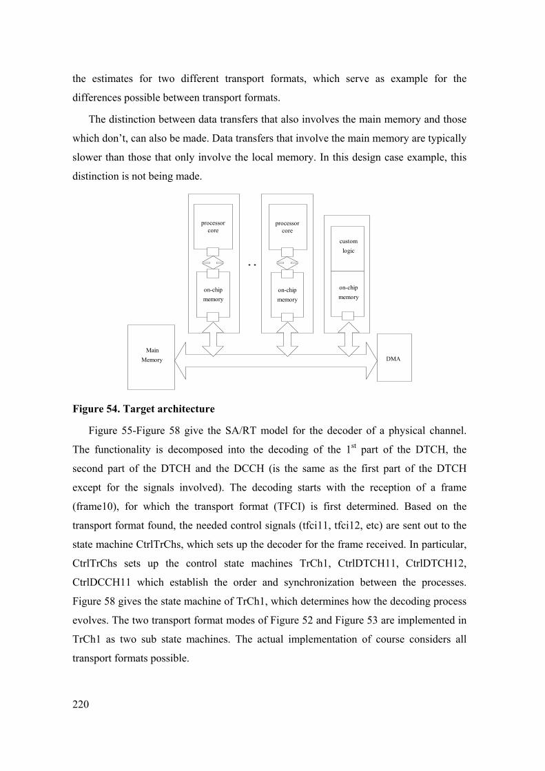
220
the estimates for two different transport formats, which serve as example for the
differences possible between transport formats.
The distinction between data transfers that also involves the main memory and those
which don’t, can also be made. Data transfers that involve the main memory are typically
slower than those that only involve the local memory. In this design case example, this
distinction is not being made.
MainMemory
processorcore
on-chipmemory
processorcore
on-chipmemory
customlogic
DMA
on-chipmemory
Figure 54. Target architecture
Figure 55-Figure 58 give the SA/RT model for the decoder of a physical channel.
The functionality is decomposed into the decoding of the 1st part of the DTCH, the
second part of the DTCH and the DCCH (is the same as the first part of the DTCH
except for the signals involved). The decoding starts with the reception of a frame
(frame10), for which the transport format (TFCI) is first determined. Based on the
transport format found, the needed control signals (tfci11, tfci12, etc) are sent out to the
state machine CtrlTrChs, which sets up the decoder for the frame received. In particular,
CtrlTrChs sets up the control state machines TrCh1, CtrlDTCH11, CtrlDTCH12,
CtrlDCCH11 which establish the order and synchronization between the processes.
Figure 58 gives the state machine of TrCh1, which determines how the decoding process
evolves. The two transport format modes of Figure 52 and Figure 53 are implemented in
TrCh1 as two sub state machines. The actual implementation of course considers all
transport formats possible.
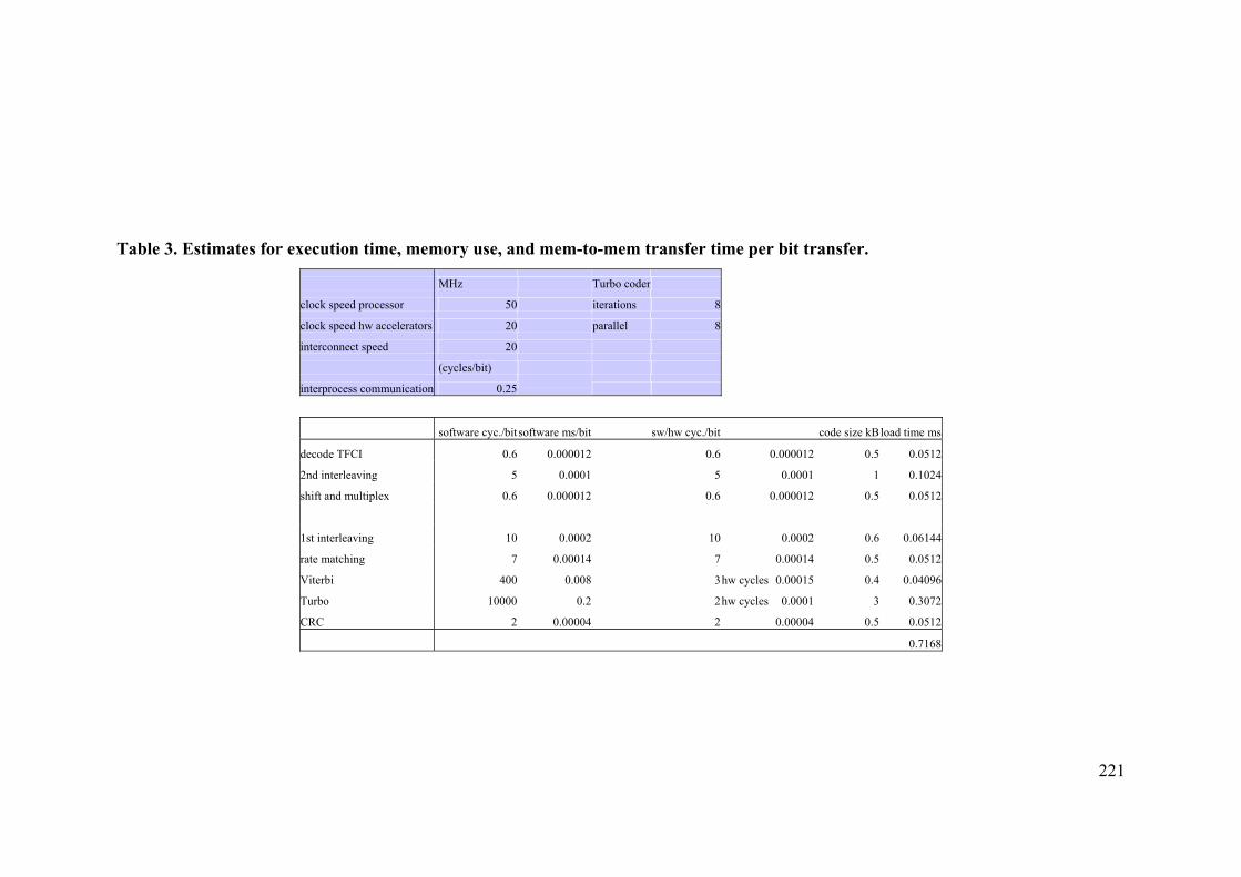
221
Table 3. Estimates for execution time, memory use, and mem-to-mem transfer time per bit transfer.
MHz Turbo coder
clock speed processor 50 iterations 8
clock speed hw accelerators 20 parallel 8
interconnect speed 20
(cycles/bit)
interprocess communication 0.25
software cyc./bit software ms/bit sw/hw cyc./bit code size kBload time ms
decode TFCI 0.6 0.000012 0.6 0.000012 0.5 0.0512
2nd interleaving 5 0.0001 5 0.0001 1 0.1024
shift and multiplex 0.6 0.000012 0.6 0.000012 0.5 0.0512
1st interleaving 10 0.0002 10 0.0002 0.6 0.06144
rate matching 7 0.00014 7 0.00014 0.5 0.0512
Viterbi 400 0.008 3 hw cycles 0.00015 0.4 0.04096
Turbo 10000 0.2 2 hw cycles 0.0001 3 0.3072
CRC 2 0.00004 2 0.00004 0.5 0.0512
0.7168

222
Table 4. Estimates for execution time, memory use, and mem-to-mem transfer time per frame transfer.
384 kbps (fig. A8 of 3GPP 25.10) DTCH bitssw (ms) hw/sw (ms)data transfer DCCH bitsSw (ms)hw/sw (ms)data transfer
decode TFCI 9120 0.10944 0.10944 0.114
2nd interleaving 9049 0.9049 0.9049 0.1131125
shift and multiplex 9049 0.108588 0.108588 0.1131125
1st interleaving 9049 1.8098 1.8098 0.1131125 284 0.0568 0.0568 0.00355
rate matching 11568 1.61952 1.61952 0.1446 360 0.0504 0.0504 0.0045
Viterbi 0 0 0 0 360 2.88 0.054 0.0045
Turbo 11568 2313.6 1.1568 0.1446 0 0 0 0
CRC 3840 0.1536 0.1536 0.048 100 0.004 0.004 0.00125
Software only solution (ms) 2318.305848 2.9912
Software plus hardware solution (ms) 5.862648 0.1652
Communication costs 0.7905375 0.0138
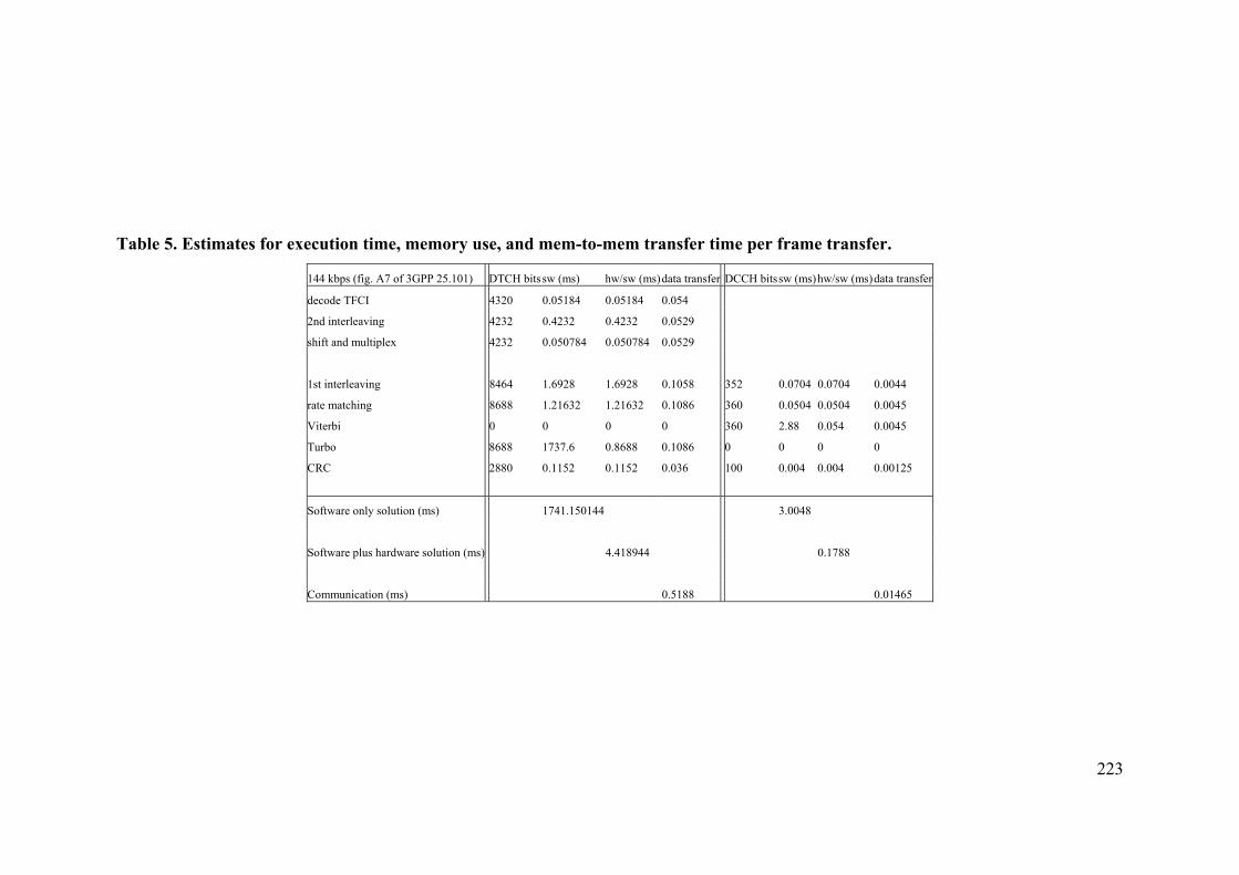
223
Table 5. Estimates for execution time, memory use, and mem-to-mem transfer time per frame transfer.
144 kbps (fig. A7 of 3GPP 25.101) DTCH bitssw (ms) hw/sw (ms)data transfer DCCH bitssw (ms)hw/sw (ms)data transfer
decode TFCI 4320 0.05184 0.05184 0.054
2nd interleaving 4232 0.4232 0.4232 0.0529
shift and multiplex 4232 0.050784 0.050784 0.0529
1st interleaving 8464 1.6928 1.6928 0.1058 352 0.0704 0.0704 0.0044
rate matching 8688 1.21632 1.21632 0.1086 360 0.0504 0.0504 0.0045
Viterbi 0 0 0 0 360 2.88 0.054 0.0045
Turbo 8688 1737.6 0.8688 0.1086 0 0 0 0
CRC 2880 0.1152 0.1152 0.036 100 0.004 0.004 0.00125
Software only solution (ms) 1741.150144 3.0048
Software plus hardware solution (ms) 4.418944 0.1788
Communication (ms) 0.5188 0.01465
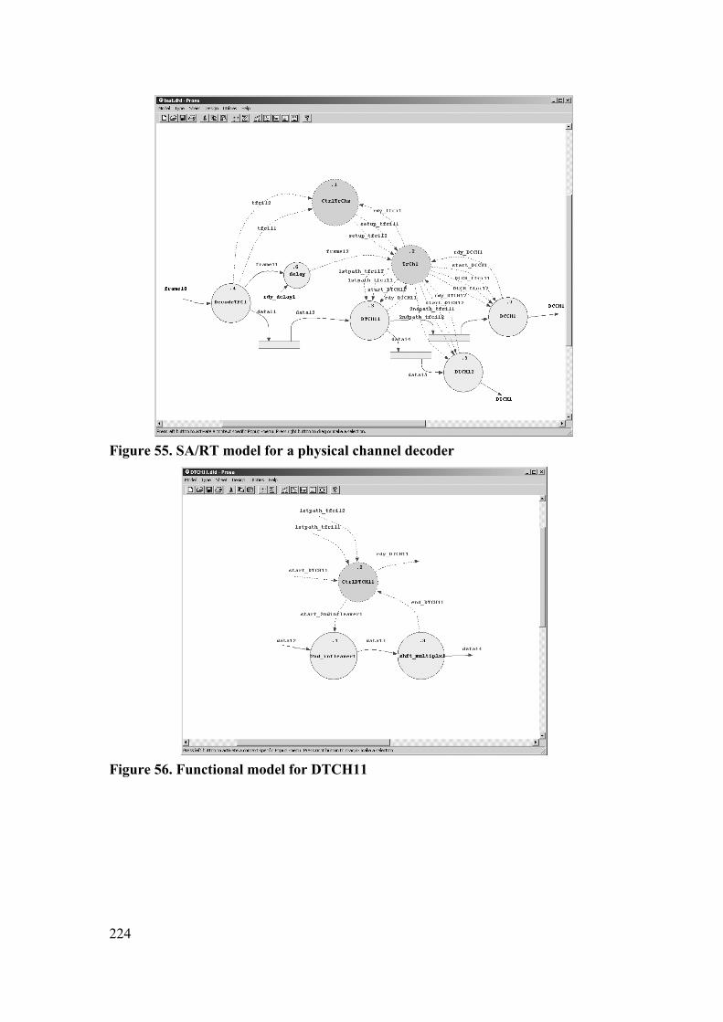
224
Figure 55. SA/RT model for a physical channel decoder
Figure 56. Functional model for DTCH11
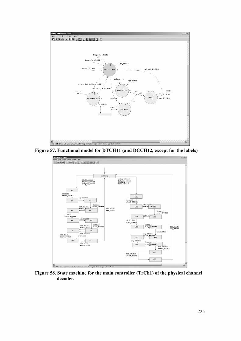
225
Figure 57. Functional model for DTCH11 (and DCCH12, except for the labels)
Figure 58. State machine for the main controller (TrCh1) of the physical channel
decoder.

226
Figure 59. Reachability graph for TrCh1, DTCH11, DTCH12, DCCH11
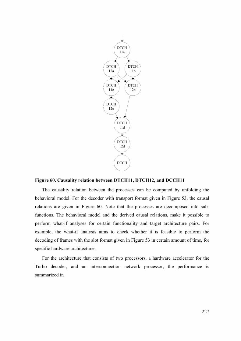
227
DTCH11a
DTCH12a
DTCH11b
DTCH12b
DTCH11c
DTCH11d
DTCH12c
DTCH12d
DCCH
Figure 60. Causality relation between DTCH11, DTCH12, and DCCH11
The causality relation between the processes can be computed by unfolding the
behavioral model. For the decoder with transport format given in Figure 53, the causal
relations are given in Figure 60. Note that the processes are decomposed into sub-
functions. The behavioral model and the derived causal relations, make it possible to
perform what-if analyses for certain functionality and target architecture pairs. For
example, the what-if analysis aims to check whether it is feasible to perform the
decoding of frames with the slot format given in Figure 53 in certain amount of time, for
specific hardware architectures.
For the architecture that consists of two processors, a hardware accelerator for the
Turbo decoder, and an interconnection network processor, the performance is
summarized in
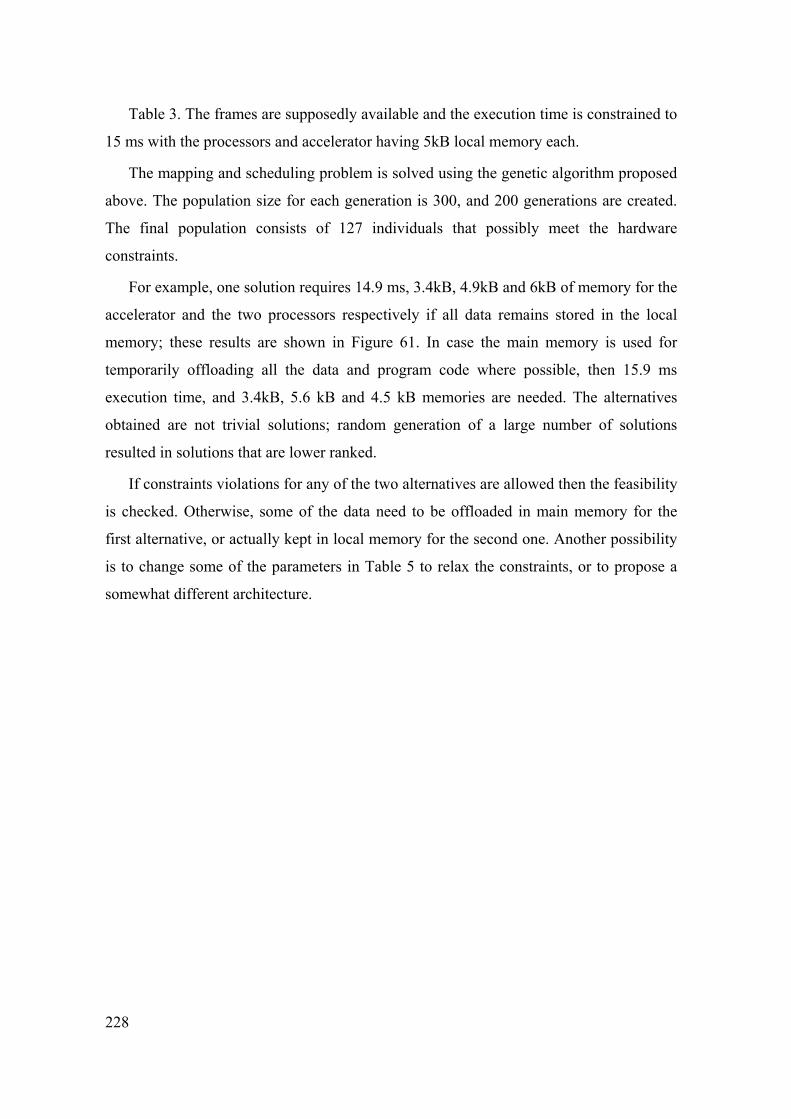
228
Table 3. The frames are supposedly available and the execution time is constrained to
15 ms with the processors and accelerator having 5kB local memory each.
The mapping and scheduling problem is solved using the genetic algorithm proposed
above. The population size for each generation is 300, and 200 generations are created.
The final population consists of 127 individuals that possibly meet the hardware
constraints.
For example, one solution requires 14.9 ms, 3.4kB, 4.9kB and 6kB of memory for the
accelerator and the two processors respectively if all data remains stored in the local
memory; these results are shown in Figure 61. In case the main memory is used for
temporarily offloading all the data and program code where possible, then 15.9 ms
execution time, and 3.4kB, 5.6 kB and 4.5 kB memories are needed. The alternatives
obtained are not trivial solutions; random generation of a large number of solutions
resulted in solutions that are lower ranked.
If constraints violations for any of the two alternatives are allowed then the feasibility
is checked. Otherwise, some of the data need to be offloaded in main memory for the
first alternative, or actually kept in local memory for the second one. Another possibility
is to change some of the parameters in Table 5 to relax the constraints, or to propose a
somewhat different architecture.
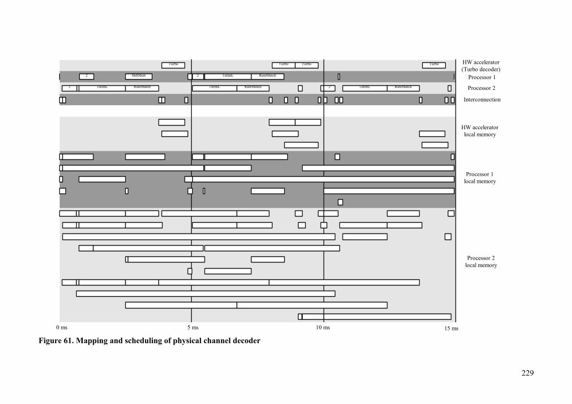
229
HW accelerator(Turbo decoder)
Processor 1
Processor 2
Interconnection
HW acceleratorlocal memory
Processor 1local memory
Processor 2local memory
0 ms 5 ms 10 ms 15 ms
Turbo Turbo
2
2 RateMatchShftMult 2 1stIntL
1stIntL RateMatch 1stIntL RateMatch 2 1stIntL RateMatch
Turbo Turbo
Figure 61. Mapping and scheduling of physical channel decoder


231
Acknowledgements
I would like to thank my promotors prof. M.P.J. Stevens for his guidance and utmost
to help with every problem during my research, and prof.dr.ir. R.H.J.M. Otten for his
solutions. I could not have done the research without the help of copromoter and project
leader dr.ir. L. Jóźwiak, hereby my thanks.
I appreciate very much the discussions with prof. K. Kuchcinski, prof. J.L. van
Meerbergen and prof. P. Pulli, and their cooperation.
I must reserve many thanks for all members of Eindhoven University of Technology
(EB group), VTT Electronics (Kari Tiensyrjä, Johan Plomp, EDA group), and Nokia
Research Center (Timo Yli-Pietilä, Risto Suoranta, DSP group).
Finally, I would like to say thanks to my family and to my mother, Anne Ong in
particular.


