Bulkowski’s Position SizingDecember 3, 2012 5:00 am1 commentViews: 1282

Position Sizing Background

For most of my investing career, I used a fixed dollar amount for money management when buying stocks. At the beginning, it was $2,000. That bought me 100 shares of a $20 stock. I thought that’s the method that everyone used. As I learned about the stock market, I knew that there were better ways to position sizing (money management) but I didn’t know what they were.

In the August 2007 issue of Active Trader magazine, Volker Knapp (see Trading system lab: “Percent volatility money management”) tested a system that used volatility to determine the position size. I already use volatility to determine stop placement (see Stop Placement), so this was a welcome addition. The article was based on Van K. Tharp’s book Trade Your Way to Financial Freedom.

 

Percent Risk Position Sizing

The first method, percent risk position sizing, is well known and it’s based on risk to determine the position size. For example, if you are looking to buy a stock with a price of $20 and a stop loss of $19, with a maximum loss of $2,000, you should buy 2,000 shares.

The formula for this approach is:

DollarRiskSize/(BuyPrice – StopPrice)

In this example, the DollarRiskSize is $2,000, the BuyPrice is $20 and the StopPrice is 19 giving a result of $2,000/($20 – $19) or 2,000 shares.

 

Percent Volatility Position Sizing

The percent volatility position sizing method adjusts the risk according to the stock’s volatility. Tests described in the article say it performs much better than the percent risk method.

Here’s the formula.

PositionSize = (CE * %PE) / SV

Where CE is the current account equity (size of portfolio)

%PE is the percentage of portfolio equity to risk per trade.

SV is the stock’s volatility (10-day EMA of the true range).

For example, if the current account equity (CE) is $100,000, the percent of portfolio equity we want to risk (%PE) is 2%, and the stock’s volatility is $1.25, then the result is: ($100,000 * 2%) / $1.25 or 1,600 shares.

Instead of calculating the 10-day exponential moving average of the true range, I just calculate the volatility using Patternz, which provides it at the click of a button.

The downfall of these two methods is that if your portfolio is $100,000, then the trade just described would chew up 1,600 shares x $20 buy price or $32,000. Thus, you can buy just over 3 stocks, giving you a concentrated portfolio. The percent-risk method would be even worse with $40,000 used for just one stock. (Of course this assumes that the stocks share the same buy price, volatility, and so on).

One way to avoid the concentrated portfolio problem is to divide the $100,000 into $10,000 allotments (or whatever size you feel comfortable with that would lead to a diversified portfolio), one for each stock. Use the same formula to determine the share size. In the percent volatility example, the computation would be: ($10,000 x 2%) / 1.25 or 160 shares.

I don’t know what this does to the profitability of the method because the article’s author didn’t discuss this. In any case, this page is about position sizing and not portfolio theory.

 

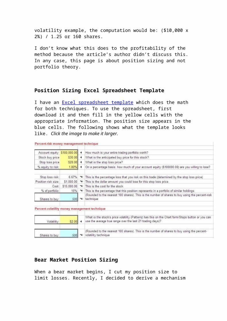
Position Sizing Excel Spreadsheet Template

I have an Excel spreadsheet template which does the math for both techniques. To use the spreadsheet, first download it and then fill in the yellow cells with the appropriate information. The position size appears in the blue cells. The following shows what the template looks like. Click the image to make it larger.

 

Bear Market Position Sizing

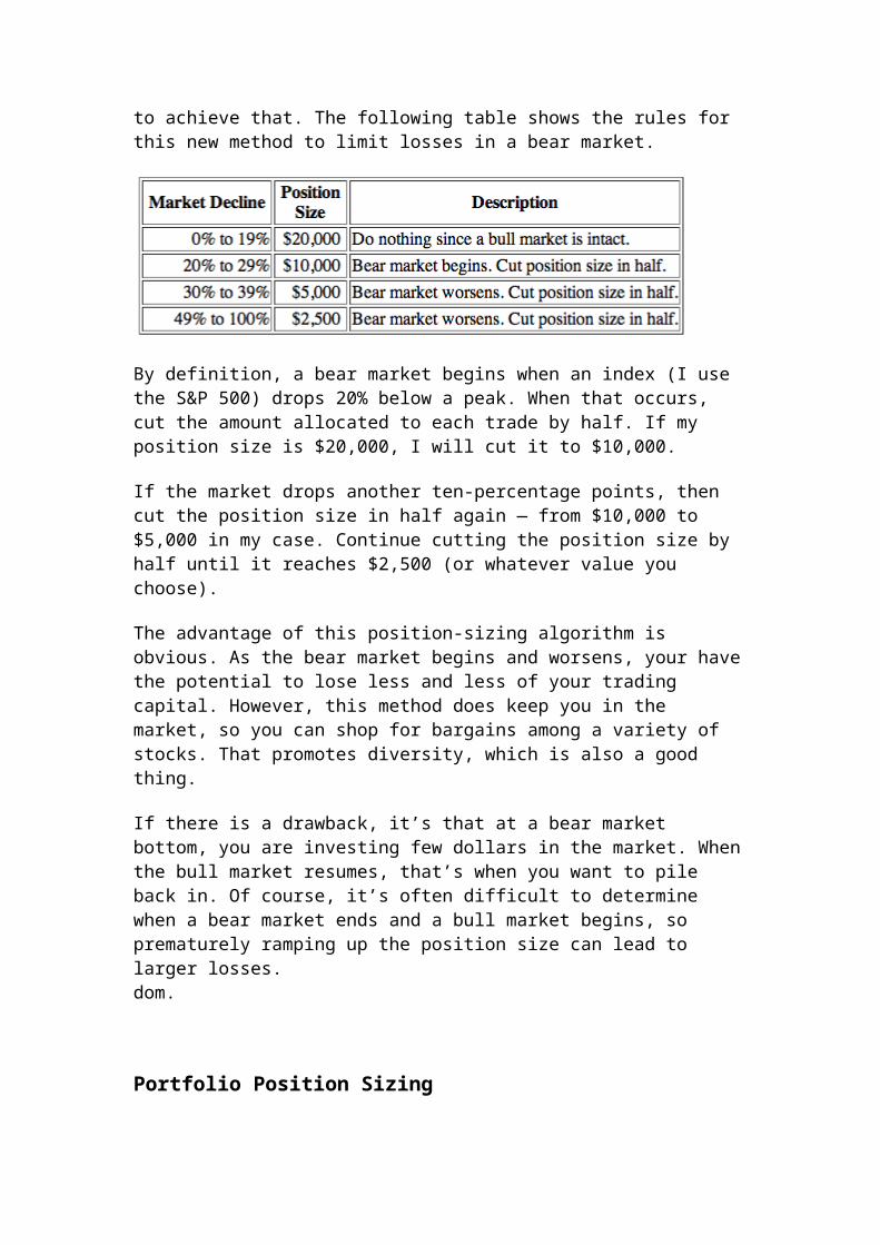
When a bear market begins, I cut my position size to limit losses. Recently, I decided to derive a mechanism to achieve that. The following table shows the rules for this new method to limit losses in a bear market.

By definition, a bear market begins when an index (I use the S&P 500) drops 20% below a peak. When that occurs, cut the amount allocated to each trade by half. If my position size is $20,000, I will cut it to $10,000.

If the market drops another ten-percentage points, then cut the position size in half again — from $10,000 to $5,000 in my case. Continue cutting the position size by half until it reaches $2,500 (or whatever value you choose).

The advantage of this position-sizing algorithm is obvious. As the bear market begins and worsens, your have the potential to lose less and less of your trading capital. However, this method does keep you in the market, so you can shop for bargains among a variety of stocks. That promotes diversity, which is also a good thing.

If there is a drawback, it’s that at a bear market bottom, you are investing few dollars in the market. When the bull market resumes, that’s when you want to pile back in. Of course, it’s often difficult to determine when a bear market ends and a bull market begins, so prematurely ramping up the position size can lead to larger losses.dom.

 

Portfolio Position Sizing

How do you size the positions in your portfolio, assuming you wish to make multiple buys per stock (or just once)?

To get the position size (shown in the above table as $20,000 then $10,000), take the value of the trading account and divide it by the number of positions you want to hold. The number of positions you choose is up to you. Many will say to hold no more than 10 to 12 with at least 7 to 8 positions to give adequate diversity. As I write this, I own 22 positions with an eye to 30. Think of this as my own private mutual fund. I’m a skilled investor/trader with 30+ years of experience, so owning this many is not a problem…but that’s just me.

For example, say you have a portfolio currently valued at $300,000, and want to hold 30 positions, then each position would be $10,000. Within 20% of a bull market peak, you’d start with 10k per position. When the bear market begins, you’d cut that in half, to 5k and then 2.5k as the bear market worsens.

That gives you the amount to invest in each stock. Now, let’s adjust the position for volatility. The more volatile the stock the fewer shares you should own.dom.

 

 Shares Per Trade

I saw one algorithm that compared the current stock’s volatility with its historical range. The “current” period used a 10-day high-low calculation but they didn’t specify what was meant by “historical.” In their example, they said “a few years ago” (whatever that means).

That bothered me. A company could have had a drug failure, dropping the stock by 70% in one session (huge historical volatility) and then sold the division. You might not know that unless you read the press releases or discovered it some other way.

I have a better idea. Why not compare the stock’s volatility to the market’s? Here’s the formula.

 Shares = (PositionSize * (MarketVolatility / StockVolatility)) / StockPrice

PositionSize comes from the above table, so it’s adjusted for the market conditions.

MarketVolatility is the daily change of the market over the last month, averaged, expressed as a percentage.

StockVolatility is the daily change of the stock over the last month, averaged, expressed as a percentage.

For the two volatility calculations, I calculate the high-low difference of the stock or market index (I use the S&P 500 index) each day for 22 trading days (about a month), average it, and divide it by the most recent close. This is nearly the same calculation that I use for a volatility stop, so check that link for an example. You can use the ATR, but it’s not as effective.

This will give you the number of shares to invest per position. You can have multiple positions per stock.

In short, take the ratio of the two volatilities to further adjust the bucks you spend and divide that by the current share price to get the number of shares.dom.

 

Volatility Stop

We adjusted the amount spent per trade for the market conditions, and then we adjusted the number of shares for the stock’s volatility. The third leg of the algorithm is to use a volatility stop. That calculates a stop loss order based on a stock’s volatility in a manner similar to the above volatility calculation.

Thus, you have three pieces: Adjusting the position size for the market conditions, adjusting it for the stock’s volatility versus the market’s, and using a volatility stop to limit losses.dom.

 

Position Sizing Example

Let’s assume we want to buy Gap (GPS) stock. It closed Friday, December 17, at 21.19. Our portfolio has a current value of $100,000 and we want to hold 10 stocks in the portfolio.

The S&P index is down less than 20% from it’s high a few days ago (it’s down less than 1% from the high). Thus, we’d spend the full $10,000 for this trade (that’s $100,000 / 10 stocks = $10,000). To find the number of shares, the market volatility is 0.009 (0.9%) and the stock’s volatility is 0.0213 (2.1%) — I have a program that calculates the two volatilities automatically. Plugging this into the formula, we get,

Shares = ($10,000 * (0.009 / 0.0213)) / 21.19 or 200 shares (I round up to the nearest 100 shares). They would be worth 200 * 21.19 or $4,238.

The volatility stop would be placed at 20.15, or 5% below the current close.

That gives us plenty of dollars to spend on the stock sometime in the future, to increase the position. The volatility and portfolio value will have changed by then, so you’d run another calculation to get the next investment amount.

— Tom Bulkowski

Measuring Success: Key Performance MetricsNovember 26, 2012 5:00 am8 commentsViews: 2480

When you see the performance of a trading system, how do you know it’s good? How do you know it’s the right system for you? Many people simply look at the net profit assuming the system with the more profit must be the better system. This is often far from a good idea. When comparing trading systems during the development process or when comparing systems before making a purchase, it is nice to have a few metrics on hand that will allow you to compare the system either to a hypothetical benchmark or against another system. There is no one single score you can use that will work for everyone since we all have unique risk tolerances and definitions on what we consider tradable. Likewise, not all scoring systems are equal or perform under all circumstances. However, in this article I’m going to talk about my favorite methods used to score and rank trading systems. These are my key system performance metrics that I use during the system development process.

Number of Trades

Any trading system should have a “significant” number of trades. What is significant? Well that varies. For a swing system that takes no more than 10 trades a year, having 100 trades is good. This represents about 10 years of historical testing. As a given trading system starts to produce more trades per year, I would expect to see more trades utilized during backtesting.

Profit Factor

While net profit can be a factor in your decision about a particular trading system, profit factor is often even more important in my opinion. Profit factor measures the efficiency of your trading system. Profit factor is calculated by dividing the generated profit by the generated losses. A profit factor of 1.5 indicates for every two dollars lost, three dollars are gained ($3 win / $2 lost = 1.5).  Obviously a number above 1.0 means you are making money. I like to see a profit factor of 1.5 or higher.

Average Profit Per Trade

Like profit factor, the average profit per trade tells me if a system is making enough money on each trade. When designing a trading system I like to see an average profitable trade above $50 before commissions and slippage are deducted at an absolute minimum. If the average net profit is above $50 with commissions and slippage deducted, that’s even better. The higher the average profit per trade the better.

Percent Winning Trades

I don’t follow this too much. I make note of it but it’s not all that important to me. The percent winning trades is simply the number of trades that generated a positive net profit divided by all trades taken. This factor can be important if you don’t like to have a large string of losers. For example, often longer term trend following systems can be very profitable, but only have a win rate of 40% or less. Can you handle many losing trades? Maybe you are only comfortable with systems that tend to produce more winning trades than losing trades. If so, then a system with a win rate of 60% or higher would be better for you. Percent winning trades is a psychological tolerance indicator that will vary between people.

Compounded Annual Growth Rate (CAGR)

This describes the growth as if it were a steady, fixed rate of return. Obviously this does not happen when trading as your trading system produces a jagged equity curve over time. Yet, this is a way to smooth your return over the same trading period. Let’s say your trading system produces a 5% CAGR over a 10 year period. Over that same period you have a bank CD that also yields a 5% return over the same time frame. Does this make the CD a better investment? Maybe. One thing to keep in mind is this: the CAGR calculation does not take into account the time your money is at risk. For example, while the trading system may be retuning 5% CAGR over 10 years, your money is only actively in the market for a fraction of the time. Most of the time it’s sitting idle in your brokerage or futures account waiting for the next trading signal. CAGR does not take into account the time your money is at risk. Remember, a 5% return in the CD is realized only if your money is locked away 100% of the time. With our example trading system our cash is also freed up to be put to use in other instruments.

Risk Adjusted Return (RAR)

This calculation takes into account the time your money is at risk in the market. This is done by taking the CAGR and dividing it by exposure. Exposure is the percentage of time (over the test period) that your money was actively in the market. I like to see a value of 50% or better.

Maximum Intraday Drawdown and The Equity Curve

How big are those drawdowns? Can I mentally handle such a drawdown?  Along these lines I also look at the shape of the equity curve. Does it climb with shallow

pullbacks or does it have steep pullbacks? Are there long extended periods with no new equity highs? Ideally, the equity curve should rise as time goes by, creating new equity highs with shallow pullbacks.

t-Test

This is one you don’t see much of. The t-Test is a statistical test used to gage how likely your trading system’s results occurred by chance alone. You would like to see a value greater than 1.6 which indicates the trading results are more likely to not be based on chance. Any other value below indicates the trading results might be based upon chance. The t-Test value should be calculated with no less than 30 trades. Below is the t-Test calculation.

t = square root ( number of trades ) * (average profit per trade trade / standard deviation of trades)

Expectancy

Expectancy is a concept that was described in Van Tharps book “Trade Your Way To Financial Freedom”. Expectancy tells you on average how much you expect to make per dollar at risk. Expectancy might also be a value that you optimize when testing different strategy input combinations. While computing the true expectancy of a trading system is beyond this article, it can be estimated with the following simple formula.

Expectancy = Average Net Profit Per Trade / | Average losing trade in dollars |

For those no too familiar with mathematics, the vertical lines around the “Average losing trade in dollars” indicates the absolute value should be used. This simply means if the number is a negative value, we drop the negative sign thus making the value positive.

Expectancy Score

This value is an annualized expectancy value which produces an objective number that can be used in comparing various trading systems. In essence the Expectancy Score factors in “opportunity” into the value by taking into account how frequently the given trading system produces trades. Thus, this score allows you to compare very different trading systems. The higher the expectancy the more profitable the system.

Expectancy Score = Expectancy * Number of Trades * 365 / Number of strategy trading days

Conclusion

With the above values we can get a decent picture on how the system will perform. There are, of course, other values you could evaluate and even more you can do such as passing the historical trades through a Monte Carlo simulator. But these values

discussed in this article are the important values I utilize when designing a system or when evaluating a third party trading system.

Building A Better Trend FilterNovember 12, 2012 5:00 am8 commentsViews: 3189

In this article I will create a trend filter (also known as market mode filter or regime filter) that is adaptable to volatility and utilizes some of the basic principles of hysteresis to reduce false signals (whipsaws). As you may know, I often will use the 200-period simple moving average (200-SMA) to determine when a market is within a bull or bear mode on a daily chart. When price closes above our 200-SMA we are in a bull market. Likewise, when price is below our 200-SMA we are in a bear market. Naturally, such rules will create some false signals. By the end of this article you will have a market mode filter that can be used in your system development that may produce better results than a standard 200-SMA filter. To build our better market trend filter we will use the following concepts:

Hysteresis Price proxy

Hysteresis Basics

When building trading systems many of the decisions have a binary outcome. For example, the market is bearish or bullish. You take the trade or you don’t. Introducing a “gray area” is not always considered. In this article I’m going to introduce a concept called Hysteresis and how it can be applied to our trading. Hysteresis was used in a previous article on reducing whipsaws within a moving average crossover trading system. While the word Hysteresis was not used specifically in that article, it was a good example.

The common analogy to help understand the concept of hysteresis is to imagine how a thermostat works. Let’s say we are living in a cool weather climate and we are using a thermostat to keep the temperature of a room at 70 degrees F (critical threshold). When the temperature falls below our critical threshold the heaters turn on and begin blowing warm air into the room. Taking this literally as soon as the temperature moves to 69.9 our heater kicks on and begins blowing warm air into the room driving the temperature up. Once the temperature reaches 70.0 our heaters turn off. In a short time the room begins to cool and our heaters must turn on again. What we have is a system that is constantly turning off and on to keep the temperature at 70 degrees. This is inefficient as it produces a lot of wear on the mechanical components and wastes fuel. As you might have guessed, hysteresis is a way to correct this issue. More in just a moment.

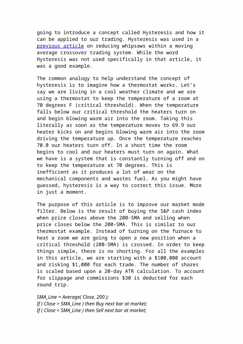
The purpose of this article is to improve our market mode filter. Below is the result of buying the S&P cash index when price closes above the 200-SMA and selling when price closes below the 200-SMA. This is similar to our thermostat example. Instead of turning on the furnace to heat a room we are going to open a new position when a critical threshold (200-SMA) is crossed. In order to keep things simple, there is no shorting. For all the examples in this article, we are starting with a $100,000 account and risking $1,000 for each trade. The number of shares is scaled based upon a 20-day ATR calculation. To account for slippage and commissions $30 is deducted for each round trip.

SMA_Line = Average( Close, 200 );If ( Close > SMA_Line ) then Buy next bar at market;If ( Close < SMA_Line ) then Sell next bar at market;

In the above image we can see we entered into the market six times before the trade moves significantly in our favor. The first five attempts were closed at a loss as price moved from bull territory back to bear territory. That’s five consecutive losing trades!

Trading Bands

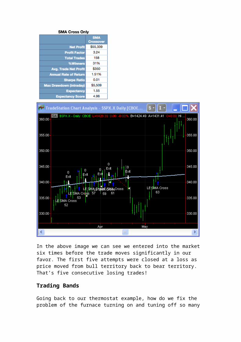
Going back to our thermostat example, how do we fix the problem of the furnace turning on and tuning off so many times? How do we reduce the number of signals? Let’s create a zone around our ideal temperature of 70 degrees. This zone will turn on the heaters when the temperature reaches 69 degrees and turn off when the temperature reaches 71 degrees. Our ideal temperature is in the middle of a band with the upper band at 71 and the lower band at 69. The lower band is when we turn on the

furnace and the upper band is when we turn off the furnace. The zone in the middle is our hysteresis.

In our thermostat example we are reducing “whipsaws” or false signals, by providing hysteresis around our ideal temperature of 70 degrees. Let’s use the concept of hysteresis to attempt to remove some of these false signals. But like our ideal temperature we want an upper band and a lower band to designate our “lines in the sand” where we take action. There are many ways to create these bands. For simplicity let’s create the bands from the price extremes for each bar. That is, for our upper band we will use the 200-SMA of the daily highs and for the lower band we will use the 200-SMA of the daily lows. This band floats around our ideal point which is the 200-SMA. Both the upper and lower bands vary based upon the recent past. In short, our system has memory and adjusts to expanding or contracting volatility. The EasyLanguage code for our new system look something like this:

SMA_Line = Average( Close, 200 );UpperBand = Average( High, 200 );LowerBand = Average( Low, 200 );If ( Close crosses over UpperBand ) then Buy next bar at market;If ( Close crosses under LowerBand ) then Sell next bar at market;

Below is a screen shot showing the effect of opening a new trade after the daily bar closes above the upper band. We have reduced our five consecutive losing trades down to two trades.

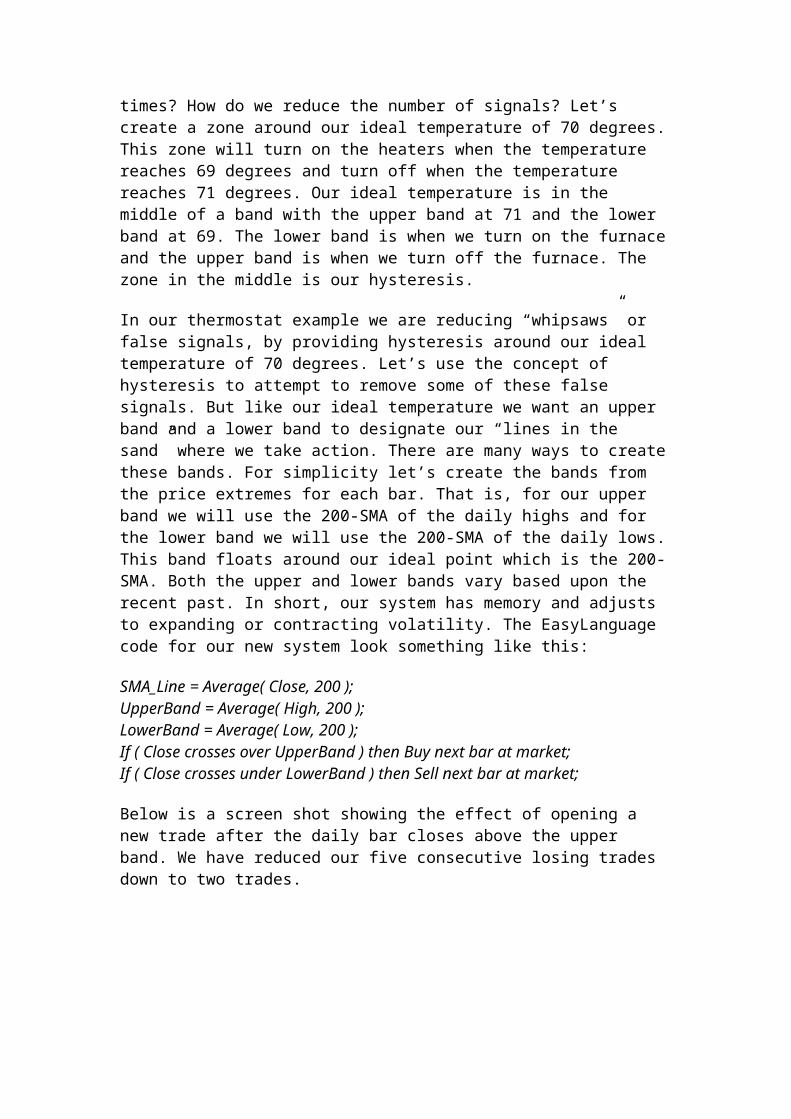
Here are the results with using our new bands as trigger points.

Looking at the performance table above we can see an improvement in nearly all aspects of the system’s key performance. Most notably, increased Net Profit, Profit Factor, Percent Winners  and Average Trade net Profit. We also reduced the number of trades and the number of consecutive losing trades. In the end we really end up with about the same amount of net profit but we accomplish this task with fewer, more profitable trades.

It’s interesting to note that our Expectancy Score falls even as we increase the Expectancy value from 1.55 to 1.71. This is due to the reduced number of trading opportunities.

Price Proxy

A price proxy is nothing more than using the result of a price-based indicator instead of price directly. This is often done to smooth price. There are many ways to smooth price. I won’t get into them here. Such a topic is great for another article. For now, we can smooth our daily price by using a fast period exponential moving average (EMA). Let’s pick a 5-day EMA (5-EMA). Each day we compute the 5-EMA and it’s this value that must be above or below our trigger thresholds. By using the EMA as a proxy for our price we are attempting to remove some of the noise of the daily price fluctuations.

Below is what the EasyLanguage code may look like.

SMA_Line = Average( Close, 200 );UpperBand = Average( High, 200 );LowerBand = Average( Low, 200 );PriceProxy = XAverage( Close, 5 );

If ( PriceProxy crosses over UpperBand ) then Buy next bar at market;If ( PriceProxy crosses under LowerBand ) then Sell next bar at market;

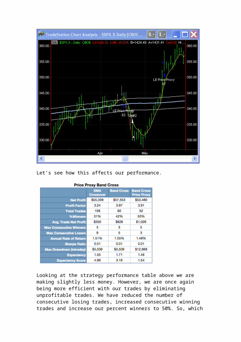
Below is an example of a trade entry. Notice the trade is opened when our price proxy (yellow line) crosses over the upper band. We have also reduced our losing trades to one.

Let’s see how this affects our performance.

Looking at the strategy performance table above we are making slightly less money. However, we are once again being more efficient with our trades by eliminating unprofitable trades. We have reduced the number of consecutive losing trades,

increased consecutive winning trades and increase our percent winners to 50%. So, which strategy is better? It all depends on what you want or what you are comfortable with. Some people will wish to simply take as much money as possible. Others will wish to reduce the number of consecutive losing trades.

The above examples are designed to demonstrate the effect a “better” trend filter can have on a simple trading strategy. If we want to use this in a trading system it would be ideal to create a function from this code that would pass back if we are in a bear or bull trend. However, the programming aspect of such a task is really beyond the scope of this article. Nonetheless, below is a quick example of setting two boolean variables (in EasyLanguage) that could be used as trend flags:

BullMarket = PriceProxy > UpperBand;BearMarket = PriceProxy <= LowerBand;

In this article we have created a dynamic trend filter that smooths price, adapts to market volatility and utilizes hysteresis principles. With just a few lines of code we can significantly reduced the number of false signals commonly associated with this style of trading strategy . This type of filter can be effective in building the trading systems for ETFs, futures and Forex.

Download

TradeStation Strategy Code (ELD file)TradeStation WorkSpace (TWS file)Strategy Code (text file)  

Jeff Swanson

Jeff is the founder of System Trader Success – an inBox magazine dedicated to sharing great ideas and concepts from the world of automated trading systems. Read More Google

System Optimization With ExpectancyOctober 1, 2012 5:00 am4 commentsViews: 563

In a recent article called Rank Your Trading System With Expectancy Score I discussed the concept of expectancy and expectancy score and how they can be used to help evaluate and compare the profitability of trading systems. In this article I’m going to provide some EasyLanguage code that will help you compute these values for a trading system and how to optimize a trading system based on expectancy. This article will be heavily geared towards TradeSation’s EasyLanguage, however the concepts can be applied to any programming language.

Expectancy Function

In the previous article I showed you how to compute both expectancy and the expectancy score. Here I want to provide you an EasyLanguage function that will do it for you. This code can be used when building your own systems or when evaluating trading systems where you have access to the code. Basically, if you have access to the code you can use this function. The function is called _CE_Expectancy and it uses the formula discussed in the previous article to calculate an expectancy. This function provides a quick way to calculate both expectancy values easily.

Place this function at the very bottom of the strategy code and execute your strategy. The function with then perform two things. First, it will populate two variables (oExpectancy and oExpectancySctore) with the expectancy value and expectancy score value. Second, if the Display boolean is set to true, the two expectancy values will be displayed within the TradeStation output window. If you don’t have Display set to true, the two expectancy values are not displayed but are accessible within the two output variables, oExpectancy and oExpectancySctore.

Below are the function input parameters as they appear in the code:

float oExpectancy(NumericRef), // Output: Expectancyfloat oExpectancyScore(NumericRef), // Output: Expectancy Scorebool Display(Truefalsesimple); // Display results or not

Below is an example of using the function within a strategy. The first two input parameters will be the expectancy values. You can use these variables to display the values or send them to a file. The last parameter tells the function not to display the expectancy values in the TradeStation print log:

RetrunVal = _CE_Expectancy( vExpectancy, vExpectancyScore, false );

Below is a video where I give a demonstration on using the expectancy function.

Expectancy Optimizer

In the previous article I hinted that you could use expectancy score as the key value to optimize a trading system against. Many people will use net profit or average profit per trade, but expectancy score might be useful as well. The expectancy score includes trading opportunity (as defined by the frequency of trading) its calculation. However, there is a problem. TradeStation provides no way to optimize over expectancy score. It must be done manually. To aid in this process I created a simple function called _CE_Expectancy_Optimizer.

This function can be added to the bottom of any trading code and is designed to help you optimize a single parameter. For example, let’s say you wish to optimize the RSI look-back period for a particular strategy. After adding the function and configuring the required parameters, you perform your TradeStation optimization as you normally would. After each iteration of the TradeStation optimizer a line is written to an Excel file which contains the current RSI look-back period, expectancy and expectancy score. You can then use Excel’s sort feature to sort the different optimization iterations based upon the expectancy score.

There is nothing fancy about the Excel document generated. In fact, if you open up this file you will find no headers or description. This is due to this function being called each time an optimization run is performed. I found no quick way to add headers only once.

Below are the function input parameters:

iWriteFlag( TrueFalseSeries ), // Should we write to a file or not?iFileName(string), // File nameiSystemName( string ), // Name of system to testiSystemVersionNumber( string ), // System's version numberiOptimize(NumericSimple); // The strategy input value you are optimizing

Here is an example of using the function within a strategy:

vRetValue = _CE_Expectancy_Optimizer( iWriteToFile, vFileName, RegimeLookback );

Below is a video demonstration of the _CE_Expectancy_Optimizer function.

Conclusion

With these two functions you will have two tools needed to calculate both the expectancy and expectancy score for the trading systems you are developing.

Downloads

The following download link contains both expectancy functions.

Expectancy Functions (TradeStation ELD)Expectancy Function (Text file)Expectancy Optimizer (Text file)

Rank Your Trading System With Expectancy ScoreSeptember 24, 2012 5:00 am10 commentsViews: 2803

In a previous article called “System Performance and Confidence Interval“, I showed how a statistical method could be used to analyze historical trading results to give us an idea if the system would likely fail in the future. In this article I would like to introduce a mathematical formula which can be applied to any trading system and used as an objective score to compare and rank different trading systems.

When it comes to trading systems, no two are alike. There is a vast number of different trading styles that cover the range from simple tick scalping to multi year investment models. Of course, there is a huge number of different instruments and

markets to trade. How would one determine if two different trading systems that trade different markets with different trading styles make an informed choice on which system was more profitable? How do you compare two trading systems’ performances? If two trading systems are both profitable and both seem like good systems, is there a single metric that can be used to compare the profitability between each?

Expectancy

Expectancy is a concept that was described in Van Tharp’s book Trade Your Way To Financial Freedom. Expectancy tells you on average how much you expect to make per dollar at risk. For example, if you have a trading system that has a .50 Expectancy that means for every dollar you risk the trading system returns $.50.

There are two ways to compute Expectancy. Both methods are simple but one requires a little more explanation but does give a more conservative answer. The second method is a bit more straightforward to explain but only give an approximation of Expectancy. However, this approximation is good enough for what we are attempting to accomplish here.

Often you will find expectancy is computed with the following formula:

Expectancy = (AW * PW + AL * PL ) / | AL | Where: AW = Average winning trade in dollars PW = Probability of winning trades | AL | = Absolute value of the average losing trade in dollars PL= Probability of losing trades

But if you look carefully at the calculation within the parenthesis you will see the value is nothing more than the trading system’s average net profit per trade. Substituting this value gives us the simplified formula of:

Expectancy = Average Net Profit Per Trade / | AL |

The two values you plug into the Expectancy formula can be found on most (if not all) strategy performance reports generated by backtesting. This is certainly true for TradeStation‘s strategy reports.

Now that we have our trading system’s Expectancy value are we ready to use this value to compare to other trading systems? Not yet. There is another step we must first take. Our Expectancy value simply tells us our historical profit per dollar risked for each trade. But we are missing something. Let’s imagine we have two trading systems that have two different Expectancy values:

Trading System #1 has an Expectancy of .25Trading System #2 has an Expectancy of .50

Based on what we know it appears Trading System #2 produces more profit per dollar risked on each trade. In fact, it produces twice as much profit per dollar risked. Thus, if we risked $500 on each trade, Trading System 1 would generate $125 dollars while

Trading System #2 would generate $250. But this not the complete picture. We are missing the frequency at which each trading system operates. For example, maybe Trading System #1 trades once per day while Trading System #2 trades once per week. We need to take into account the number of times the trading system trades over the number of days the system was tested. In Van Tharp’s book he described that as Expectancy multiplied by opportunity. Opportunity is nothing more than how often does a given trading system trade. Opportunity times Expectancy leads us to our final calculation for Expectancy Score.

Expectancy Score

This value is an annualized Expectancy value which produces an objective number that can be used in comparing various trading systems. In essence the Expectancy Score factors in a trading system’s trade frequency. The higher the Expectancy Score the more profitable the system. This final score allows you to compare very different trading systems.

Expectancy Score = Expectancy * Number of Trades * 365 / Days in historical test

The Number of strategy trading days is nothing more than the number of days your backtesting was performed.

Conclusion

With the Expectancy Score in hand we have a metric to aid us in comparing different trading systems. Other uses for Expectancy Score might also include using this value as a target for optimization. Often optimization is performed on net profit, profit factor, Sharpe ratio or other metrics. Using Expectancy may also be something worth pursuing. But how would you do that using TradeStation? Unfortunately, there is no easy way to do it with TradeStation. However, I’m working on some EasyLanguage code that will help with a manual process. More on that in a future issue.

Step One In Building An Intraday Trading SystemAugust 6, 2012 5:00 am5 commentsViews: 2017

If you have been reading System Trader Success for a few months you’re probably familiar with how I develop trading systems. The very first step is to come up with a simple idea to act as the seed or core of your trading system. I call this your key concept. This key concept is a simple observation of market behavior. This observation does not need to be complex at all. In fact, they are often very simple. For example, here is a key concept: most opening gaps on the S&P market close if the gaps are less than 4 points. This key concept is very simple, and testable. From this key concept there is an entire process of building a trading system which I described in the free ebook,  How To Develop Profitable Trading Systems.

Testing An Intraday Key Concept

Today I want to show you a tool I use to help test key ideas on an intraday chart. Building trading systems on intraday charts (day-trading systems) are some of the more difficult systems to develop when compared to daily charts. First, you must deal with more market noise but even more dangerous is slippage and commissions. Why? Your potential profit per trade is small on a day trading system thus, both commissions and slippage take a bigger bite out of your profits (as a percentage of your P&L) and produce more drag on the performance of your system. The hill you’re climbing is a lot steeper when creating a day trading system.

They Key Concept

For this example let’s create a simple trend following strategy for the Euro currency futures (EC) market on a 5-minute chart. We’ll use the extreme readings on the RSI indicator as our signal. Because we are using RSI as a trend indicator that means we are looking to enter the market when RSI gives us an extreme reading. That is, go-long at the oversold region (RSI value above 80) and go-short at the lower region (RSI value below 20). This is a bit unconventional, but when it comes to the markets, unconventional can be beneficial. As for the extreme values, those are unoptimized numbers. I just picked them off the top of my head in hopes of looking for a strong swing in ether direction.

Below is the EasyLanguage code for the key concept.

MyRSI = RSI( Close, RSILookBack ); If ( MyRSI < ShortZone ) ThenbeginGoShort = true;GoLong = false;End Else If ( MyRSI > BuyZone ) ThenBeginGoShort = false;GoLong = true;End; If ( MP = 0 ) Then BeginIf ( GoShort and BullTrend ) Then Sellshort (“RSI Short”) next bar marketElse If ( GoLong and BearTrend ) Then Buy(“RSI Buy”) next bar at market;End;

If you code this basic concept up and test it from 0830 to 1500 (central) on the EC market what do you think you’ll get? That’s right, a losing concept with an ugly equity curve.

Take Every RSI Signal

Clearly, we don’t want to trade our system at any time during the U.S. day session. We want to focus when EC is most likely to show strong trending characteristics. If the price of EC is strong enough to push the RSI value above 80 we want price to continue climbing. So, what market session is best suited for this RSI trend system? Or are all market sessions hopeless for this simple trading concept? Let’s find out.

Session Testing

When designing a day trading system one of the first steps I want to perform is to test which market session will likely produce the best results. We are all aware that different sessions exist for any market. For example, when dealing with the emini S&P we have a pre-market session, the morning session, lunch time session and an afternoon session. Often you can see distinct characteristics within each session. So, when I’m developing a trading system for day trading I don’t want to blindly trade during every session. I want to be more targeted in my approach. There will most likely be a particular session or two where my key concept will do better than other sessions. In order test our key idea over different sessions I needed to create an EasyLanguage strategy that can isolate these sessions and execute the key concept individually over those session only.

This is where my “Session Testing” code comes into play. Session Testing is an EasyLanguge Strategy that I wrote to help me in this task of testing various intraday sessions. Using TradeStation’s optimizer I can test my idea across different combinations of sessions and discover how the key concept holds up across each session. Here are the basic sessions:

1. “Pre-Market” Between 530 and 8302. “Open” Between 830 and 10303. “Morning”4. “Lunch” Between 1030 and 12305. “Afternoon” Between 1230 and 15006. “Close” Between 1430 and 15157. “Post-Market” Between 1500 and 18008. “Night” Between 1800 and 530

From this list of basic session I created several more “sessions” based upon combinations of the above.

1. “Pre-Market” + “Open”2. “Pre-Market” + “Open” + “Morning”3. “Open” + “Morning”4. “Open” + “Morning” + “Lunch”5. “Lunch” + “Afternoon”6. “Lunch” + “Afternoon” + “Close”7. “Daily Session”8. “Night” + “Pre-Market”9. “Morning” + “Afternoon”

The 17 different sessions I came up with may not please everyone. Perhaps you have a different idea on how to break the different sessions up and with the code provided you can simply change them to your liking. For example, if you are interested in the European markets and trade those times, you can create your own sessions based around the European markets.

Within the code you’ll find a location to put your key trading idea. This is where I placed the RSI rules. I picked a value of nine for the RSI look-back period because I wanted it to be more sensitive than the default 14 that is often used. (The value of nine really has no significance. It was not optimized and I could have very well picked seven or ten. I just simply picked it.) Also, notice I have no stops or targets within my test code. Instead the strategy simply enters a trade if the the proper condition is met and the trade is exited only at the close of the session. That’s it. Remember, I’m not testing a trading strategy. I’m testing a key concept vs. different market sessions. Our goal is to locate the best possible market sessions for my key concept. In this case, which session holds the strongest trending characteristic? Once a session(s) has been identified only then will I continue to develop a complete strategy (containing stops, targets and other rules) tailored to the top session(s).

Next let’s see what happens when I run TradeStation’s optimizer over each of the sessions. In doing so TradeStation will systematically execute my key concept strategy over each market session and record the trading results. After all the sessions have been analyzed I can generate a bar graph representing the P&L for each session. Below is the Net Profit graph which depicts the total net profit from our testing. By the way, we were testing this strategy from January 1, 2003 to December 31, 2011. This timespan covers both bull and bear markets. It’s important to test your key concept over a wide range of market conditions. Slippage and commissions are not factor into these results.

Net Profit vs Market Session

In this case we can see session input value number 12 produces the best net profit. This input value is actually a combination of Open, Morning and Lucnh sessions. It’s during these times EC market apparently demonstrates strong trending characteristics that we might be able to take advantage of with our key concept.

Let’s now isolate the session input value to 12 and execute our key concept on this specific time.  For this test I will deduct $18.50 per round trip for slippage and commissions. Below is the equity graph of our key concept along with some performance numbers.

EC RSI Trend Key Idea — Equity Curve

There is no optimization here. The code simply trades based off un-optimized RSI signals and the results look promising. Below is the Trade Summary Report.

Strategy Performance Report

There you have it. This type of RSI trend following concept should be developed for the Open, Morning and Lunch sessions. This makes sense. The big volume and big

trends often appear during the U.S. day session. This is also corroborated from a previous Best Times To Day Trade where I explored the hourly range of the Euro Currency market. In that study we can see the hours between 0800 and 1100 (Central) have the highest price movement of the EC market.

I would like to point out again, this is not a trading system. What we did in this article is validate our key concept. The code presented in this article does not have stops, a regime filter, volatility filters, profit targets or any number of other checks and balances we might see in a true trading system. In fact, take a look at the average profit per trade. It’s $24 after slippage and commissions which is too low in my opinion. I would like to see this closer to $50 per trade or higher.

What’s next? First I would begin the testing process as described in the free ebook, How To Develop Profitable Trading Systems. This would include testing testing regime filters, entry methods, trailing stops, profit targets, volatility filters and whatever else you feel might make a better system.

Summary

This simple trend following concept appears to have potential if executed on the correct market session.

This is not a trading system but a proof-of-concept. Further research and development is needed for a final system.

When developing a day trading system, take a look at the different market sessions and see if your key concept performs better in certain sessions.

Many people will try to develop an intraday system without taking into account the different market sessions. However, if you test your key trading idea across all market sessions and narrow it down to the most productive sessions, I think this will help jump start your development of a profitable system. The Session Test strategy code is available below.

Download

Session Test ELD (TradeStation)SessionTest Workspace (TradeStation)   Session Test Strategy (text file)Session Test Function (text file)  

Jeff Swanson