
The Collection Efficiency of Shielded and Unshielded Precipitation Gauges. Part II:Modeling Particle Trajectories
MATTEO COLLI AND LUCA G. LANZA
Department of Civil, Chemical and Environmental Engineering, University of Genoa, and WMO–CIMO
Lead Centre ‘‘B.Castelli’’ on Precipitation Intensity, Genoa, Italy
ROY RASMUSSEN
National Center for Atmospheric Research, Boulder, Colorado
JULIE M. THÉRIAULT
Department of Earth and Atmospheric Sciences, University of Quebec at Montreal, Montreal, Quebec, Canada
(Manuscript received 16 January 2015, in final form 18 June 2015)
ABSTRACT
Theuse ofwindshields to reduce the impact ofwind on snowmeasurements is common. This paper investigates
the catching performance of shielded and unshielded gauges using numerical simulations. In Part II, the role of
the windshield and gauge aerodynamics, as well as the varying flow field due to the turbulence generated by the
shield–gauge configuration, in reducing the catch efficiency is investigated. This builds on the computational fluid
dynamics results obtained in Part I, where the airflow patterns in the proximity of an unshielded and single Alter
shielded Geonor T-200B gauge are obtained using both time-independent [Reynolds-averaged Navier–Stokes
(RANS)] and time-dependent [large-eddy simulation (LES)] approaches. ALagrangian trajectorymodel is used
to track different types of snowflakes (wet and dry snow) and to assess the variation of the resulting gauge
catching performancewith the wind speed. The collection efficiency obtainedwith the LES approach is generally
lower than the one obtained with the RANS approach. This is because of the impact of the LES-resolved
turbulence above the gauge orifice rim. The comparison between the collection efficiency values obtained in case
of shielded and unshielded gauge validates the choice of installing a single Alter shield in a windy environment.
However, time-dependent simulations show that the propagating turbulent structures produced by the aero-
dynamic response of the upwind singleAlter blades have an impact on the collection efficiency. Comparisonwith
field observations provides the validation background for the model results.
1. Introduction
The goal of this study is to provide numerical esti-
mates of the impact of wind on the catching perfor-
mance of an unshielded and single Alter (SA) shielded
Geonor T-200B vibrating wire gauge. The work is based
on a set of underlying three-dimensional airflow fields
obtained in Colli et al. (2015a, hereafter Part I) from
computational fluid dynamics (CFD) simulations. The
modeled shield–gauge geometry is shown in Fig. 1 of
Part I. The flow patterns are derived from the solution of
the three-dimensional motion equations of the airflow
realized around a shielded and unshielded gauge under
varied undisturbed wind conditions.
Part I investigated the pattern of streamlines near the
shield–gauge configuration using two approaches, namely,
the time-invariant method based on the Reynolds-
averaged Navier–Stokes (RANS) equations and the
time-variant method based on large-eddy simulations
(LESs). Both of them provide estimates of the airflow
turbulence generated by the shield–gauge assembly within
the undisturbed laminar wind field by means of the spatial
distribution of the turbulent kinetic energy parameter k. In
addition, LES directly solves the large scales of the fluc-
tuating flow and provides time-dependent air velocity and
pressure fields (U and p, respectively). This would over-
come the limitations of previous numerical studies of the
Corresponding author address: Matteo Colli, Department of
Civil, Chemical and Environmental Engineering, University of
Genoa, Via Montallegro 1, CAP 16145 Genoa, Italy.
E-mail: [email protected]
JANUARY 2016 COLL I ET AL . 245
DOI: 10.1175/JHM-D-15-0011.1
� 2016 American Meteorological Society

catching performance of snow gauges, which are focused
on time-invariant solutions only and neglect the parti-
cle density in the calculation of the resulting collection
efficiency (Folland 1988; Ne�spor and Sevruk 1999;
Thériault et al. 2012).The RANS simulations showed that the time-averaged
wind speed upstream of the gauge is lower when using an
SA shielded gauge instead of an unshielded gauge. Higher
values ofU and kwere computed above the collector in an
unshielded configurationwhen compared to the SA shield.
The paired RANS simulation and LES highlighted a
general underestimation of turbulence by the former
model just above the gauge orifice rim. The time-variant
analysis clearly showed that propagating turbulent
structures generated by the aerodynamic response of the
upwind SA blades have a relevant impact on the k fields
above the gauge collector (Part I). The actual impact of
this on the expected undercatch can only be evaluated
after tracking the precipitation particles.
In this paper, we use a Lagrangian tracking model
(LTM) to calculate the collection performance of
unshielded and SA shielded precipitation gauges. The
LTM predicts the snowflake trajectories starting from
the underlying airflow fields computed by both RANS
simulation and LES. The first part of the analysis fol-
lows the methodology proposed by Thériault et al.
(2012) to address a comparative evaluation of the
catching performance of shielded and unshielded
gauges with the RANS time-invariant approach. In a
second instance, the impact of time-variant airflows on
the trajectories is investigated by means of a modified
LTM, based on the LES outputs. This is a novel anal-
ysis of the impact of fluctuating air velocity fields onto
the trajectory model for the SA shielded gauge.
2. Method
a. Calculation of the collection efficiency
The catching performance of the snow gauges is cal-
culated by running numerical simulations of the trajec-
tories for a number of snowflake types and sizes. This is
possible by assuming the particle physical characteristics
as described by a general power law (Rasmussen et al.
1999) in the form
X(dp)5 a
XdbXp , (1)
where dp is the particle diameter and X assumes the
nomenclature of the particle terminal velocity wT , vol-
ume Vp, bulk density rp, and cross-sectional area Ap.
For the sake of simplicity, we categorize the hydrome-
teors as wet and dry snow only. In a second step, we in-
tegrate the results over a proper particle size distribution
(PSD) for the hydrometeors in order to obtain gauge
performance at any given precipitation rate.
The values of the parameters aX and bX are provided in
Table 1. This parameterization was employed by Thériaultet al. (2012) for the LTM simulations, obtaining a good
agreement between the modeled and in-field observations
at the Marshall test site, Colorado, with data properly
classified by crystal types using a photographic technique.
Although modifications are necessary to study the
effect of time-variant flow fields and to improve the
calculation of the gauges’ undercatch in mass-weighted
terms, the LTM follows Ne�spor and Sevruk (1999) and
Thériault et al. (2012). The tracking algorithm is based
on the equation of motion
Vprpap52
1
2C
DA
pra(v
p2 v
a)jv
p2 v
aj1V
p(r
p2 r
a)g ,
(2)
where ap is the snowflake acceleration, g is the gravity
acceleration, CD is the drag coefficient, Vp is the particle
volume,Ap is the cross sectional area, and ra and rp are the
density of the air and the snow particles. Solving Eq. (2) for
the particle-to-air magnitude of velocity vector, we obtain
jvp2 v
aj5 [(u
p2 u
a)2 1 (y
p2 y
a)2 1 (w
p2w
a)2]1/2, (3)
where u, y, and w represent the streamwise, crosswise,
and vertical components of velocity. The three compo-
nents of the particle acceleration from Eq. (2) are
apx52
1
2C
DA
p
ra
Vprp
(up2 u
a)jv
p2 v
aj , (4a)
apy52
1
2C
DA
p
ra
Vprp
(yp2 y
a)jv
p2 v
aj, and (4b)
apz52
1
2C
DA
p
ra
Vprp
(wp2w
a)jv
p2 v
aj1
(rp2 r
a)
rp
g ,
(4c)
where the x, y, and z subscripts mark the streamwise,
crosswise, and vertical components of particle acceler-
ation and the third equation has an additional term g
to consider the gravity force in the vertical particle
TABLE 1. Parameters aX and bX of Eq. (1) (Rasmussen et al.
1999) for the computation of the snowflake terminal velocity
(i.e., wT), volume (i.e., Vp), bulk density (i.e., rp), and cross-
sectional area (i.e., Ap).
awTbwT
aVpbVp
arp brp aApbAp
Dry snow 107 0.2 p/6 3 0.017 21 p/4 2
Wet snow 214 0.2 p/6 3 0.072 21 p/4 2
246 JOURNAL OF HYDROMETEOROLOGY VOLUME 17

acceleration. While the drag coefficient of a falling
particle is influenced by the instantaneous particle-to-air
magnitude of velocity through the particle Reynolds
number (Stout et al. 1995; Ne�spor and Sevruk 1999), the
present methodology adopts the simplification of using a
fixed CD during the particle motion calculated as a
function of the particle terminal velocity given as
CD5
2Vp(r
p2 r
a)g
Apraw2
T
. (5)
The influence of turbulence on the particle drag is ig-
nored in this formulation. Although this formulation would
be exact in the case of stagnant air, we are neglecting the
bond between turbulence and the particle drag (the drag
curve). The work of Thériault et al. (2012) demonstrated
that this hypothesis does not lead to relevant inaccuracies.
Considering that the volume and the density of the snow-
flakes are a function of dp, following Eq. (1) we obtain the
CD formulation as
CD5
2gaVparp
aApraawT
d(bVp
1brp2bAp
22bwT)
p . (6)
Thériault et al. (2012) report on the theoreticalCD curves
as a function of dp for various types of snowflake crystals
using the Rasmussen parameterization (Rasmussen
et al. 1999) and including dry and wet snow as reported
in Table 1. Equation (6) shows a general decrease of
the particle drag with increasing diameter; the inertial
forces of the larger particles dominate the viscous ef-
fects with trajectories that are theoretically less con-
ditioned by the airflow conditions. The trajectories are
therefore easily computed with a forward steps pro-
cedure for a given snowflake type, dp, and free-stream
velocityUw by calculating at short time intervals Dt thevariations of the particle position until the trajectory
remains in the proximity of the gauge. This is achieved
by the following set of equations:
Dx5 x22 x
15
�up11
1
2axDt
�Dt , (7a)
Dy5 y22 y
15
�yp11
1
2ayDt
�Dt, and (7b)
Dz5 z22 z
15
�w
p111
2azDt
�Dt , (7c)
where x1, y1, and z1 and x2, y2, and z2 are, respectively, the
previous and the new spatial coordinates of the particle. The
velocity components assigned to the new particle position
(up2 , yp2 , and wp2 ) are updated by adding the following
increments to the previous step values:
Dup5 u
p22 u
p15 a
xDt , (8a)
Dyp5 y
p22 y
p15 a
yDt, and (8b)
Dwp5w
p22w
p15 a
zDt . (8c)
Note that from Eq. (4) the acceleration vector ai at the
ith time step is dependent on the particle-to-air velocity
difference vp 2 va, meaning that an interpolation scheme
of the air velocity gridded values to the exact xi has to be
applied. This is acceptable considering the high spatial
resolution of the mesh in the vicinity of the windshield
and the gauge bodies, where the velocity gradients are
larger. The Lagrangian procedure does not handle the
collisions between particles since trajectories are solved
independently from each other.
To reduce the computational burden of the simulation,
only a reduced number of trajectories within the spatial
domain are simulated. The choice of the initial particle
locations determines the simulated trajectories. The ini-
tial positions of the simulated trajectories lay on an ideal
vertical plane located upwind of the windshield and the
orifice level. Figure 1 shows the selected seeding window
and its location relative to the shield–gauge assembly.
The seeding window is oriented crosswise to the un-
disturbed wind field, at a fixed distance upstream of the
gauge, but with variable elevation with respect to the
collector as a function of the wind velocity, the crystal
type, and the particle diameter.
To calculate the wind-induced undercatch, we as-
sume, as in Thériault et al. (2012), an inverse exponen-
tial PSD of the hydrometeors in the form
N(dp)5N
0exp(2Ld
p) , (9)
FIG. 1. Positioning of the seeding window (product of length L
and height H) at a fixed streamwise distance xw upstream of the
gauge orifice and variable elevation zw with respect to the collector.
JANUARY 2016 COLL I ET AL . 247
where N0 (mm21m23) is the intercept parameter, L(mm21) is the slope, and dp is the particle diameter.
Ne�spor (1995) defined the gauge catching performance
for a specific dp/Uw combination as the catch ratio r
(unitless), here defined as
r5A
inside(d
p,U
w)
Agauge
, (10)
where Ainside(dp, Uw) is the effective collecting area
associated with the number of particles collected by
the gauge and Agauge(dp, Uw) is the area associated
with the entering particles in case of undisturbed
airflow.
The catching performance of the snow gauges are here
quantified by the collection efficiency (CE) variable.We
estimate CE starting from a particle counting technique
as in Thériault et al. (2012), with an integral formulation
expressed as
CE(Uw)5
ðdpmax
0
Ainside
(dp,U
w)N(d
p)d
pðdpmax
0
Agauge
N(dp)d
p
. (11)
However, the investigated gauge actually measures the
equivalent depth (or volume) of precipitation by
weighing the water entering the orifice area. To ensure
that theoretical results can be compared with in-field
estimates of the collection efficiency, it was assumed that
the density of snow varies with dp, yielding
CE(Uw)5
ðdpmax
0
Vw(d
p)A
inside(d
p,U
w)N(d
p)d
pðdpmax
0
Vw(d
p)A
gaugeN(d
p)d
p
, (12)
with Vw(dp) denoting the equivalent water volume.
The new (mass weighed) formulation for the collection
efficiency, here called the volumetric method, highlights
a double dependency of CE on the particle diameter
through their volume and the density as well. That is, we
account for the actual volume of the collected pre-
cipitation in CE, the analysis being now consistent with
the formulation provided in terms of precipitation rate by
Ne�spor and Sevruk (1999) and the in-field measure-
ments, expressed with the usual volumetric per unit area
dimensions.
b. Experimental design
The trajectory model is run initially with the un-
derlying RANS airflow in the shielded and unshielded
configurations. The model is initialized with the air
velocity vectors obtained from the CFD results without
accounting for the simulated turbulent kinetic energy
fields. Therefore, our time-averaged approach only con-
siders turbulence in averaged terms, that is, insofar as it
affects themean airflow.Multiple runs are produced for a
set of 10wind speeds (Uw 5 1–10ms21) and two different
crystal types (representative of wet and dry snow) as in
Thériault et al. (2012). The trajectory results provide the
necessary information to compute the CE(Uw) curve
using the volumetric integration method [Eq. (12)].
The time-dependent approach is different and is
computationally heavier. The velocity vectors are in-
deed refreshed, using the LES outputs at every 0.05 s.
MultipleLESwere produced for the SA shieldedGeonor.
Eight wind speeds (Uw 5 1–8ms21) were simulated at
1ms21 increments, for both wet and dry snow.
In the time-dependent configuration, we estimated
the overall CE over the total time by repeating the tra-
jectories’ computation with six starting times, which
employed different initial airflow configurations. The
use of the particle tracking algorithm within a time-
dependent approach required implementation of a re-
fined version of the LTM. The time-dependent LTM
provides six sets of trajectories yielding six collection
efficiency values (based on the volumetric integration
method) for each tested wind speed and crystal type.
The resulting CE curves derive from the average values
of these six runs at each wind speed, while their dis-
persion provides an indication of the time dependency
of the problem.
3. Results and discussion
a. Comparison of shielded and unshielded time-averaged results
We initially considered a set of trajectories based on the
time-invariant airflow fields for the unshielded and the SA
shielded gauge configurations. The resulting dataset in-
cludes multiple simulations for varying undisturbed wind
speed, particle diameter, and crystal type.
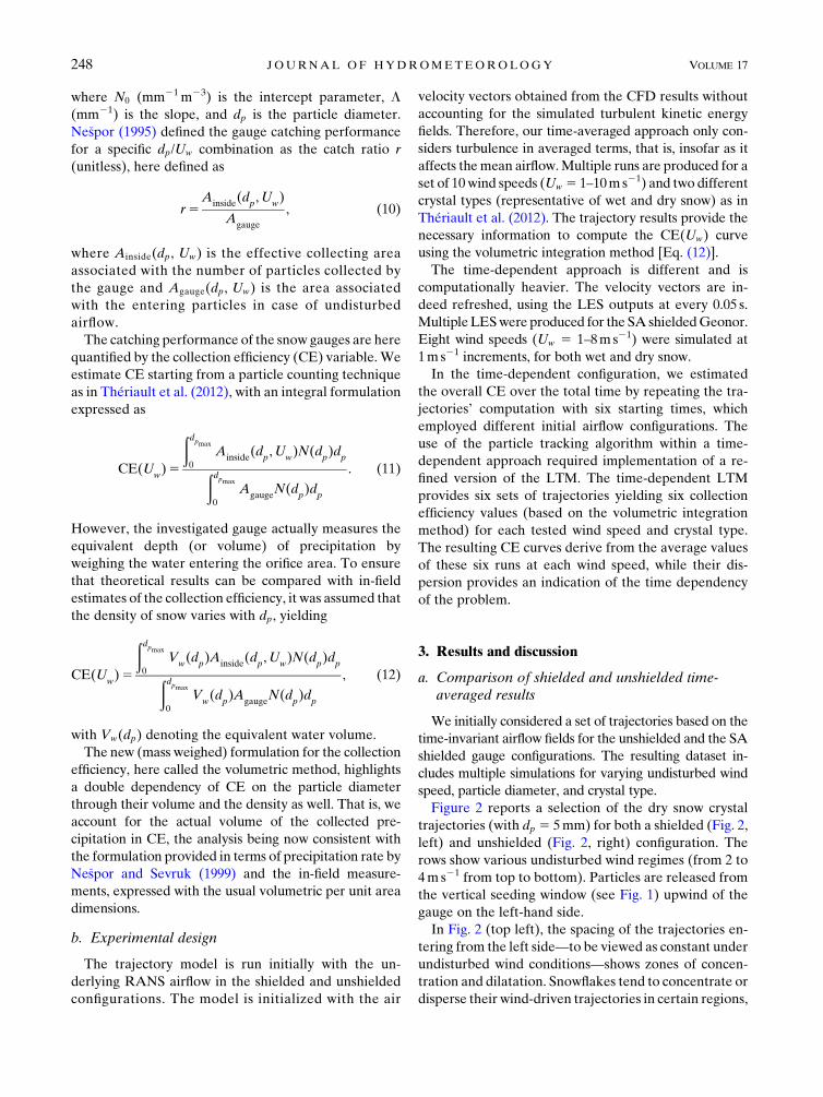
Figure 2 reports a selection of the dry snow crystal
trajectories (with dp 5 5mm) for both a shielded (Fig. 2,
left) and unshielded (Fig. 2, right) configuration. The
rows show various undisturbed wind regimes (from 2 to
4ms21 from top to bottom). Particles are released from
the vertical seeding window (see Fig. 1) upwind of the
gauge on the left-hand side.
In Fig. 2 (top left), the spacing of the trajectories en-
tering from the left side—to be viewed as constant under
undisturbed wind conditions—shows zones of concen-
tration and dilatation. Snowflakes tend to concentrate or
disperse their wind-driven trajectories in certain regions,
248 JOURNAL OF HYDROMETEOROLOGY VOLUME 17

depending on the local configuration of the air velocity
field. As described in Part I, significant local air velocity
gradients and strong updrafts occur in the region be-
tween the upstream shield blades and the gauge collec-
tor. The updraft is strong enough to shift the particle
trajectories upward, while the free space above the
shield–gauge configuration shows a relevant horizontal
air velocity. When trajectories that are shifted upward
reach this zone, the upper-level airflow blocks any fur-
ther lifting of the particles, causing an accumulation of
trajectories at the level of the orifice. For this reason, the
observed concentration and dispersion of trajectories (a
feature called here the clustering effect) is caused by
the combined windshield and gauge aerodynamic in-
fluence on the particle falling paths and may play a rel-
evant role on the catch performance, depending on the
wind speed. Figure 2 (left) highlights this phenomenon
and shows that the particle cluster is dragged upward
with increasing wind speed (and the associated updraft).
At lowwind speed, the trajectories passing above the SA
shield remain mainly undisturbed until close to the
gauge orifice, with a high number of particles falling inside
the gauge. At 3ms21, the cluster of trajectories is deflected
upward and a convergence zone occurs at the level of the
gauge collector, leading to a larger number of entering
particles than at 2ms21.At 4ms21 the number of collected
particles is drastically reduced, because of the cluster shift-
ing upward, far from the gauge orifice, as a result of stronger
vertical velocities on the upstream side of the orifice. A
different scenario is reported for the unshielded Geonor
T-200B (Fig. 2, right) where the snow trajectories are
solely deflected by the action of the gauge orifice. In this
case, the number of trajectories that cross the gauge
collector gradually decreases by increasing the Uw.
A first estimate of the gauge collection capabilities
under the various RANS testing conditions is obtained
by simply counting the entering particles with respect to
the expected number in case of an undisturbed velocity
field. Figure 3 shows the catch ratios for each snowflake
diameter, providing a first estimate of the actual con-
tribution of different particle sizes to the total CE in the
case of a shielded gauge and dry snow. The gauge un-
dercatch is more evident for the lighter particles.
The lowest wind regime (Uw 5 1ms21) shows a flat
catch ratio distribution for the shielded gauge (Fig. 3a)
over the particle diameter with values varying from 0.9
to 0.95. At an intermediate wind speed (Uw 5 4ms21),
particles smaller than dp 5 4mm missed the gauge com-
pletely. Only at the largest diameter is r comparable with
the values observed under weak wind regimes. Finally, a
severe wind speed simulation (Uw 5 8ms21) confirms this
trend with null r values across the whole PSD.
Looking at the dry snow catch ratio for the unshielded
configuration (Fig. 3b), among the three representedUw
conditions, only the lowest one (Uw 5 1m s21) resulted
in r distributions that contain particles of all diameters.
The total CE(Uw) [Eq. (12)] of the unshielded and
shielded gauge is shown in Fig. 4. Large variations in the
collection efficiency are present in the SA case when
compared to the unshielded gauge. For example, the col-
lection efficiency of dry snow increases at Uw 5 3ms21
(CE 5 95%) followed by the rapid decrease to a zero
collection efficiency at 5ms21. This sharp variation is ex-
plained by the clustering effect highlighted in Fig. 2. This is
supported by the size distribution of dry snow falling in the
gauge shown in Fig. 3. For the wet snowflakes (triangle
symbols), the collection efficiency decreases gradually with
increasing wind speed without reaching zero. The wet and
dry snow CE associated with the unshielded gauge (gray
lines) is generally less than the shielded gauge. Note that,
at the highest wind regime (Uw $ 9ms21), the collection
efficiency is higher for the unshielded gauge.
FIG. 2. Deformation of the dry snowflake trajectories near the (left)
SA shielded and (right) unshielded gauge with increasing wind speed
(time-independent RANS airflows with dp 5 5mm). The seeding
window of the trajectories is located upstream of the windshield at
a nondimensional streamwise distance equal to x/D 5 26.25.
JANUARY 2016 COLL I ET AL . 249

Overall, for wet snow, the CE decreases nearly line-
arly between 1 and 8ms21 for the unshielded gauge. At
Uw . 8m s21, the CE remains constant at ’0.3. This
requires further investigation based on a wider spectrum
of dp and crystal types under severe wind regimes. Ex-
perimental observations in the field confirm such be-
havior (Colli 2014).
b. The influence of time-variant airflow patterns onthe collection efficiency
This section presents the analysis of the impact of
turbulence on the collection efficiency of an SA shielded
gauge. The work does not address the turbulence of the
incoming airflow and that generated by the rough
ground at the lower boundary, which will be the subject
of future work. As an initial attempt to include time
dependency in the numerical modeling of the CE, this
work focuses on the wind-driven turbulence generated
by the laminar flow interacting with the windshield and
the gauge geometry.
We computed various time-dependent trajectories by
varying the starting time t0 (s) of the particles within the
fluctuating flow field. The intertime period between
different runs of the LTMwas determined for each wind
speed according to the characteristic time of the turbu-
lent structures generated by the shield–gauge bodies
(Colli 2014). At 2ms21 the resulting intertime value is
equal to 0.03 s. For example, six realizations of the
FIG. 3. Dry snow catch ratio (unitless) vs the particle diameter (mm) at three wind speeds
(m s21) for the (a) SA shielded and (b) unshielded gauge based on the time-averaged (RANS)
approach.
FIG. 4. Dry (diamonds) and wet (triangles) snow CE (unitless) vs
wind speed (m s21) for the SA shielded (black lines) and unshielded
(gray lines) gauge based on the time-averaged (RANS) approach.
250 JOURNAL OF HYDROMETEOROLOGY VOLUME 17

trajectories computed by the time-dependent LTM are
shown in Fig. 5 for dry particles of 5-mm diameter at
Uw 5 2ms21. The irregular distribution of the displayed
trajectories results from the turbulent structure of the
airflow created by the shield–gauge assembly. These ir-
regular paths are particularly evident in case of dry
snow, where trajectories are strongly affected by the air
velocity and pressure gradients generated by the upwind
shield blades. The wet snow case shows a less complex
pattern of trajectories in the space between the wind-
shield and the gauge, thanks to the longer relaxation
time of this type of snowflake (Colli 2014).
Table 2 summarizes the influence of the airflow con-
figuration at the beginning of the trajectories’ computa-
tion on the evolution of the particles paths. Six collection
efficiency values CE(t0) are averaged to account for six
different LTM starting times per each tested wind speed
and crystal type. The standard deviation s and coefficient
of variation CV5s/m of CE (where m is the mean)
quantify the variability of the catching performance due
to the arbitrary choice of the initial configuration of the
evolving airflow operated by the LTM.
The dry snow case presents a larger variability of the
CE in the 2 #Uw # 5ms21 range. This is confirmed by
the values ofCV reported inTable 2 that are equal to 0.51
with Uw 5 3ms21 and 0.85 when Uw 5 4ms21. At the
higher wind speed, the significance of CV decreases be-
cause m(CE) is close or equal to zero [refer to s(CE)].
This is explained by considering the distribution of the air
velocity time series measured near the gauge orifice by
Part I. Both the horizontal and the vertical air velocity
components revealed a noticeable increase of the am-
plitude of the fluctuations when moving from Uw 5 2 to
3ms21. This enhances the influence of the airflow tur-
bulence on the snowflake trajectories and the associated
standard deviation of CE(t0).
The dispersion of the wet snow CE(t0) values with Uw
shows a different behavior, with a CV(CE) from 0.05 to
0.23 when moving from Uw 5 4 to 5m s21 and an in-
crease of CVwhenUw $ 5ms21. This is indicative of the
fact that the wet, heavier particles require stronger wind
regimes to produce the same CE(t0) variability shown
for lower air velocities with dry snow.
By averaging the six r(t0) values, we obtain the catch
ratio histograms reported in Fig. 6 (which is directly com-
parable with Fig. 3). When Uw 5 1ms21 (dark gray bars)
the gauge collects a larger number of small dry particles.
This is a consequence of the convergence of trajectories
occurring in the time-dependent implementation of the
model. Additionally, the dry snow case presents nonzero
values of r over the whole dp range at an intermediate wind
speed equal to 4ms21, even if the population of large-size
collected particles is smaller. Under the strongest wind
speed (Uw 5 8ms21), the gauge collected no dry snow.
Figure 7 illustrates the time-dependent collection ef-
ficiency curve m(CEDRY) for dry snow (black diamonds)
calculated by employing the volumetric method. The
m(CEDRY) values show again a rapid decrease between
Uw 5 2 and 3ms21, similarly to what is observed for the
time-averaged results between Uw 5 3 and 4m s21
(Fig. 2). The gray bars in the background represent the
differences (DCE) with respect to the time-averaged
solution (gray triangles). The main distinction is ob-
served at Uw 5 3m s21, where the time-averaged CE is
influenced by the convergence of trajectories crossing
the gauge collectors. Since the clusters of trajectories
originate because of the shield aerodynamics, it must be
noted that the results presented in this work are repre-
sentative of the specific SA gauge geometry.
In Fig. 8, the difference between wet snow CERANS
and CELES never exceeds DCE 5 0.12, with a good
FIG. 5. Streamwise views of the dry snowflake trajectories com-
puted with different starting times (s) with respect to the evolving
flow (intertime period equal to 0.03 s). The LTM was run with the
following setup: SA shielded Geonor T-200B, Uw 5 2m s21, dp 55mm, and LES airflow model.
JANUARY 2016 COLL I ET AL . 251

agreement between the two numerical approaches being
observed from 2 to 5ms21 owing to the slower response
time of the wet snow particles. The choice of using a
time-independent or time-dependent approach does not
affect much the estimation of the total CE for heavier
precipitation particles such as wet snowflakes.
c. Comparison with field observations
To evaluate the reliability of the current numerical
results, we compared our estimates of the CE with ob-
servations from the Haukeliseter field site (Norway).
Snowfall measurements were made by Wolff et al.
(2015) using SA shielded and unshielded Geonor gauges
and were compared to the Double Fence Intercomparison
Reference (DFIR; Yang et al. 1999; Yang 2014). The
recent results of Yang (2014) improved the DFIR es-
timate of the true snowfall (given by Tretyakov gauge
measurements made in bush fences) using Valdai data
(Russia) from 1991 to 2010 and provided updated
hbush/hDFIR versus Uw curves and regressions (where h
represents equivalent water precipitation amount).
These equations were used to adjust the DFIR mea-
surements from the Haukeliseter site to improve the
estimation of the CE values for two collocated SA
shielded gauges. Application of the experimental
curves provided by Yang (2014) to different field sites is
not rigorous since the local climatology of Valdai has
some impacts on the crystals’ composition of the snow.
However, in general terms, the reduction of the un-
certainties related to the DFIR exposure effect leads to
in-field CE estimates that are closer to the theoretical
formulation.
Figure 9 presents in-field 1-h collection efficiency
values for an SA shielded Geonor based on two envi-
ronmental temperature ranges, 08 . T . 248C (gray
dots) and T , 248C (black dots), respectively. Light
precipitation events characterized by an accumulation
lower than 0.1mm have not been included. The two
averaged CE curves obtained with time-dependent
simulations for wet and dry snow appear in the same
plot, together with the box plot distribution of CE
values. The wet snow CE curve provides a center to the
T . 248C solid precipitation observations, which is a
reasonable result. In this case, the dispersion of the CE
values around their mean due to the airflow turbu-
lence seems to explain part of the scatter in the field
observations.
The dry snow CE curve provides a lower limit for the
set of field data having T , 248C. This is somewhat
unexpected, as the dry snow curve should be intuitively
TABLE 2. Time average (i.e., m), std dev (i.e., s), and coefficient of variation (CV) of CE (unitless) computed by varying the trajectory
starting time for the wet and dry snow crystal cases.
Uw
1m s21 2m s21 3m s21 4m s21 5m s21 6m s21 7m s21 8m s21
m(CEdry) 0.85 0.96 0.33 0.15 0.07 0.01 0.01 0.01
s(CEdry) 0.02 0.08 0.17 0.13 0.05 0.00 0.00 0.01
CV(CEdry) 0.03 0.08 0.51 0.85 0.72 0.40 0.52 1.33
m(CEwet) 0.89 0.91 0.88 0.83 0.78 0.66 0.46 0.33
s(CEwet) 0.01 0.01 0.05 0.04 0.18 0.18 0.13 0.16
CV(CEwet) 0.01 0.01 0.06 0.05 0.23 0.27 0.28 0.49
FIG. 6. Dry snow catch ratio (unitless) vs particles diameter (mm) and wind speed (m s21) for
the SA shielded gauge based on the time-dependent (LES) approach.
252 JOURNAL OF HYDROMETEOROLOGY VOLUME 17

centered on the cold temperature data. It seems that
the simulated snow trajectories either have a lower-than-
observed terminal velocity leading to a lower CE, or other
factors are in play. These could be in-stream turbulence of
the airflow, or the fact that the windshield slats are here
assumed as stationary while in reality they are free to
swivel. The trend in CE is correct, however, showing that
simulation captures some of the basic interactions of the
snowflakes with the shield–gauge geometry.
In addition, the CE(Uw) curves presented in this
section demonstrated a high sensitivity of the particle
trajectories to the physical parameterization of the
crystal types (see the recurrent comparison between
dry and wet snow). Thériault et al. (2012) showed a
relevant modulation of the CE curves due to the vari-
ous snow crystal structures parameterized with the
Rasmussen et al. (1999) experimental formulation.
Note that the real-world solid precipitation can occur
with a blending of different crystal types (further to the
possible occurrence of mixed liquid and solid pre-
cipitation). In addition, Colli et al. (2015b) reported
that the assumption of different drag coefficient for-
mulations for the dry snow particles may impact the
trajectories’ model results.
On the other hand, various effects related to the
airflow can affect the consistency of the comparison
between experimental and modeled CE estimates. For
example, the contribution of the wind speed variability
over the sampling time of the snow measurements can
lead to some deviations because the variation of the
collection with wind speed is highly nonlinear. This
issue can be easily overcome by assuming a maxi-
mum value for the coefficient of variation of Uw, as
already done for the observations reported in Fig. 9
[CV(Uw), 0:2].
The use of a static spatial grid for the airflow simu-
lations is another restriction that may influence the
resulting airflow and the modeled CE curves. This
choice was because, even if the real windshield blades
are free to oscillate along the mounting ring when the
wind blows, the computational power required to
perform an LES analysis over a dynamic mesh is still
too onerous (while it may be feasible in the case of
time-independent RANS airflow modeling). It is
therefore reasonable to attribute part of the in-field
data scattering to the crystal type detection issue. This
notwithstanding, residual differences between experi-
mental and simulated CE values persist, which are
partly attributable to the approximated modeling of
the shield–gauge geometries and simplifications of the
snowflake characteristics and the tracking scheme.
FIG. 7. Dry snow CE (unitless) vs wind speed (m s21) for the SA
shielded gauge based on the time-averaged RANS and the time-
dependent LES approach (gray and black curves, respectively) and
their differences (background histograms).
FIG. 8. Wet snow CE (unitless) vs wind speed (m s21) for the SA
shielded gauge based on the time-averaged RANS and the time-
dependent LES approach (gray and black curves, respectively) and
their differences (background histograms).
FIG. 9. Comparison between in-field SA shielded (gray and black
dots) and modeled (dashed curves with box plots) CE (unitless) vs
the undisturbed horizontal wind speed (m s21). Field data are
classified based on the environmental temperature separating
precipitation occurring under 08 . T . 248C from T , 248C.
JANUARY 2016 COLL I ET AL . 253

4. Conclusions
We conducted a numerical modeling analysis of the
wind-induced undercatch of snow precipitation gauges.
The investigation focused on the weighing-type gauges
since they are widely employed for ground-based ob-
servations. We calculated snowflake trajectories by us-
ing 3D air velocity fields around an unshielded and SA
shielded Geonor T-200B vibrating wire gauge under
different wind conditions.
The wind fields derive from Part I, where we performed
a detailed CFD study of the airflow patterns past shielded
and unshielded gauges. Both time-independent (RANS)
and time-dependent (LES) models were developed to in-
vestigate the role of turbulence generated by the shield–
gauge geometry on the deformation of the snowflake
trajectories.
The time-independent comparison between CE re-
sults obtained by modeling shielded and unshielded
gauges validates the empirical choice of installing an
SA shield to improve snow measurements. The LES
approach revealed the significant time variability of
the flow. We used a Lagrangian approach to compute
the particle trajectories, assuming no impact of the
hydrometeors on the flow and disregarding the possi-
bility of collisions, coalescences, and breakups be-
tween the falling particles. The use of a mass-weighted
CE formulation accounted for the actual volume of the
collected precipitation instead of simply counting the
number of particles entering the gauge as in previous
literature.
The comparison between RANS and LES airflows
highlighted a general underestimation of the turbu-
lence just above the gauge orifice rim by the former
model, here parameterized by the turbulent kinetic
energy k. As a result, the CE from the LES approach
was lower than that derived from the RANS model.
The time-dependent simulations showed that the
propagation of the turbulent structures, produced by
the aerodynamic response of the upwind SA blades,
has an impact on the turbulent kinetic energy realized
above the gauge collector. This in turn affects the
particle trajectories.
The time-dependent CE estimates provided in this
work are appreciably lower than existing numerical
simulation results obtained by using RANS models
(Ne�spor and Sevruk 1999; Thériault et al. 2012). Thisrevealed that the turbulence generated by the shield–
gauge has an impact on the CE. Multiple runs of the
trajectories’ computation by starting the snowflake
tracking at different instants of the evolving LES
airflow demonstrated the influence of turbulence on
the particle paths. The noticeable difference between
the CE for dry and wet snow crystals demonstrates the
importance of the physical parameterization of hy-
drometeors (terminal velocity and mass). This would
represent an additional source of variability of the
CE(Uw) resulting from different empirical models of
the particle density, volume, and terminal velocity.
The impact of more accurate particle tracking
schemes on the total collection efficiency estimates
is a matter of future work.
The numerical simulation of the CE(Uw) curve
compares well with the real-world data and reveals
that the two cases of wet and dry snow help explain
the reason for the large variability in the in-field
collection efficiency estimates. The numerically cal-
culated CE from the LES runs for dry snow over-
estimated the reduction of CE with increasing Uw in
the field data.
Acknowledgments. This researchwas supported through
funding from the Ligurian District of Marine Technol-
ogy and SITEP Italia (Italy), the National Center for
Atmospheric Research (United States) NSF-funded
Water System program, and the Natural Sciences and
Engineering Research Council (NSERC) of Canada.
Field data have been provided courtesy of Dr. Mareile
Wolff and the Norwegian Meteorological Institute
(http://met.no/English/).
REFERENCES
Colli, M., 2014: Assessing the accuracy of precipitation gauges: A
CFD approach to model wind induced errors. Ph.D. thesis,
School in Science and Technology for Engineering, University
of Genova, 209 pp.
——, L. Lanza, R. Rasmussen, and J. M. Thériault, 2015a: Thecollection efficiency of shielded and unshielded precipitation
gauges. Part I: CFD airflow modeling. J. Hydrometeor., 17,231–243, doi:10.1175/JHM-D-15-0010.1.
——, R. Rasmussen, J. M. Thériault, L. Lanza, C. Baker, and
J. Kochendorfer, 2015b: An improved trajectory model to evalu-
ate the collection performance of snow gauges. J. Appl. Meteor.
Climatol., 54, 1826–1836, doi:10.1175/JAMC-D-15-0035.1.
Folland, C., 1988: Numerical models of the raingauge exposure
problem, field experiments and an improved collector design.
Quart. J. Roy. Meteor. Soc., 114, 1485–1516, doi:10.1002/
qj.49711448407.
Ne�spor, V., 1995: Investigation of wind-induced error of pre-
cipitation measurements using a three-dimensional numerical
simulation. Ph.D. thesis, Swiss Federal Institute of Technology
Zurich, 109 pp.
——, and B. Sevruk, 1999: Estimation of wind-induced error of
rainfall gauge measurements using a numerical simula-
tion. J. Atmos. Oceanic Technol., 16, 450–464, doi:10.1175/
1520-0426(1999)016,0450:EOWIEO.2.0.CO;2.
Rasmussen, R., J. Vivekanandan, J. Cole, B. Myers, and C. Masters,
1999: The estimation of snowfall rate using visibility. J. Appl.
Meteor., 38, 1542–1563, doi:10.1175/1520-0450(1999)038,1542:
TEOSRU.2.0.CO;2.
254 JOURNAL OF HYDROMETEOROLOGY VOLUME 17

Stout, J. E., S. P. Arya, and E. L. Genikhovich, 1995: The effect
of nonlinear drag on the motion and settling velocity of
heavy particles. J. Atmos. Sci., 52, 3836–3848, doi:10.1175/
1520-0469(1995)052,3836:TEONDO.2.0.CO;2.
Thériault, J., R. Rasmussen, K. Ikeda, and S. Landolt, 2012: De-
pendence of snow gauge collection efficiency on snowflake char-
acteristics. J. Appl. Meteor. Climatol., 51, 745–762, doi:10.1175/
JAMC-D-11-0116.1.
Wolff, M., K. Isaksen, A. Petersen-Øverleir, K. Ødemark, T. Reitan,
and R. Bækkan, 2015: Derivation of a new continuous
adjustment function for correcting wind-induced loss of solid
precipitation: Results of a Norwegian field study.Hydrol. Earth
Syst. Sci., 19, 951–967, doi:10.5194/hess-19-951-2015.
Yang, D., 2014: Double Fence Intercomparison Reference (DFIR)
vs. Bush Gauge for true snowfall measurement. J. Hydrol.,
509, 94–100, doi:10.1016/j.jhydrol.2013.08.052.
——, and Coauthors, 1999: Quantification of precipitation mea-
surement discontinuity induced by wind shields on na-
tional gauges. Water Resour. Res., 35, 491–508, doi:10.1029/
1998WR900042.
JANUARY 2016 COLL I ET AL . 255

Copyright of Journal of Hydrometeorology is the property of American MeteorologicalSociety and its content may not be copied or emailed to multiple sites or posted to a listservwithout the copyright holder's express written permission. However, users may print,download, or email articles for individual use.


