The Dynamic Controllability of
Simple Temporal Networks with Uncertainty
Luke HunsbergerVassar College
Poughkeepsie, NY, USA
ICAPS-2013 TutorialJune 10, 2013
Dynamic Controllability of STNUs • 1 • Luke Hunsberger
1
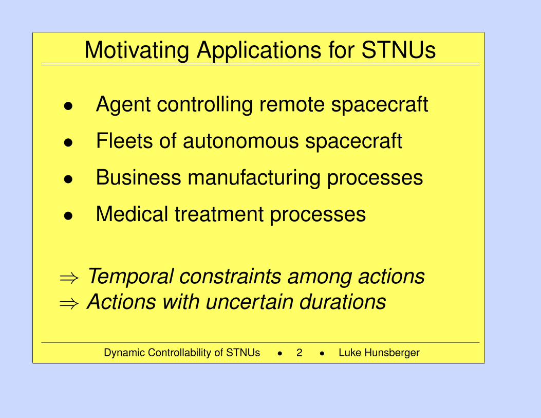
Motivating Applications for STNUs
• Agent controlling remote spacecraft
• Fleets of autonomous spacecraft
• Business manufacturing processes
• Medical treatment processes
⇒ Temporal constraints among actions⇒ Actions with uncertain durations
Dynamic Controllability of STNUs • 2 • Luke Hunsberger
2
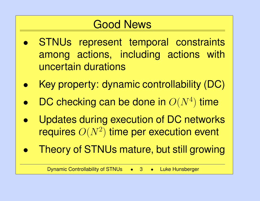
Good News• STNUs represent temporal constraints
among actions, including actions withuncertain durations
• Key property: dynamic controllability (DC)
• DC checking can be done in O(N 4) time
• Updates during execution of DC networksrequires O(N 2) time per execution event
• Theory of STNUs mature, but still growing
Dynamic Controllability of STNUs • 3 • Luke Hunsberger
3
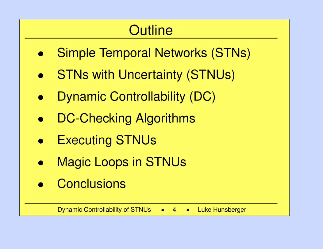
Outline
• Simple Temporal Networks (STNs)
• STNs with Uncertainty (STNUs)
• Dynamic Controllability (DC)
• DC-Checking Algorithms
• Executing STNUs
• Magic Loops in STNUs
• Conclusions
Dynamic Controllability of STNUs • 4 • Luke Hunsberger
4
Simple Temporal Networks
Dynamic Controllability of STNUs • 5 • Luke Hunsberger
5
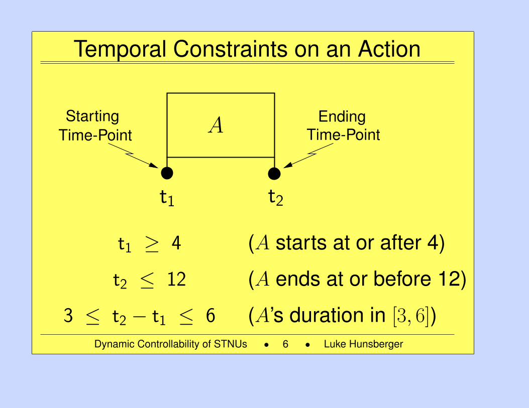
Temporal Constraints on an Action
A
t1 t2
Time-PointEnding
Time-PointStarting
t1 ≥ 4 (A starts at or after 4)
t2 ≤ 12 (A ends at or before 12)
3 ≤ t2 − t1 ≤ 6 (A’s duration in [3, 6])Dynamic Controllability of STNUs • 6 • Luke Hunsberger
6
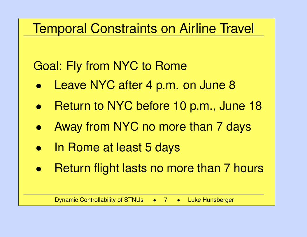
Temporal Constraints on Airline Travel
Goal: Fly from NYC to Rome
• Leave NYC after 4 p.m. on June 8
• Return to NYC before 10 p.m., June 18
• Away from NYC no more than 7 days
• In Rome at least 5 days
• Return flight lasts no more than 7 hours
Dynamic Controllability of STNUs • 7 • Luke Hunsberger
7
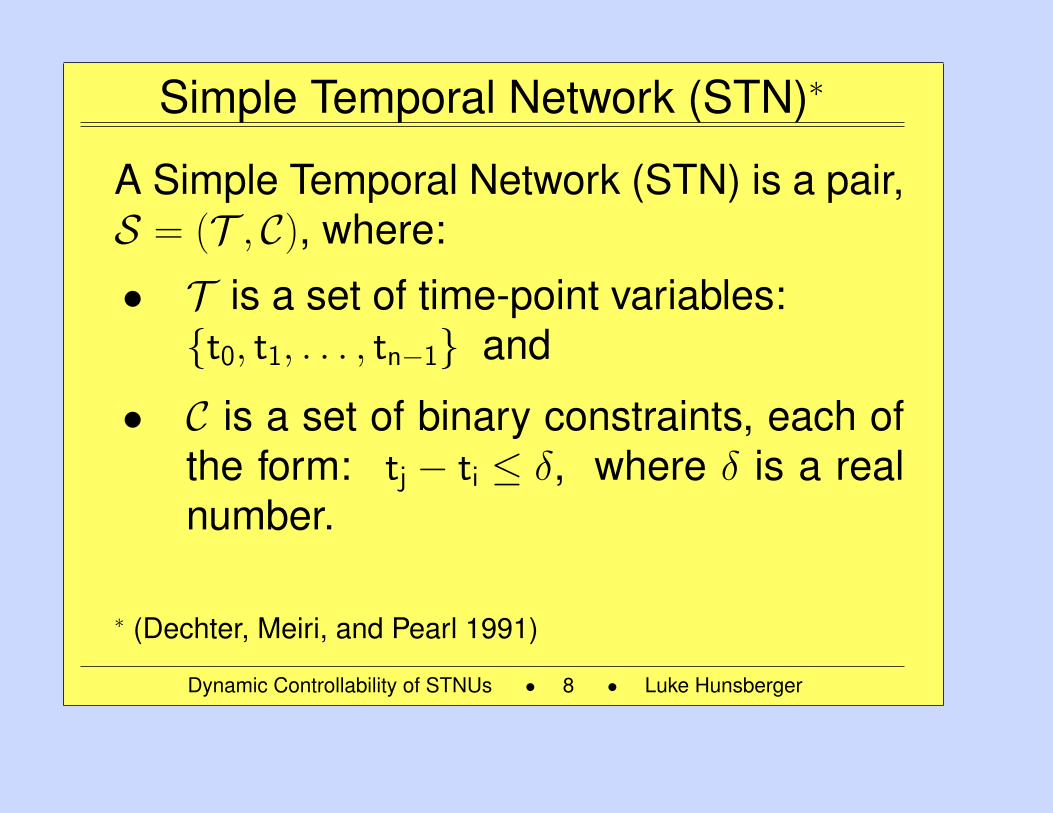
Simple Temporal Network (STN)∗
A Simple Temporal Network (STN) is a pair,S = (T , C), where:
• T is a set of time-point variables:t0, t1, . . . , tn−1 and
• C is a set of binary constraints, each ofthe form: tj − ti ≤ δ, where δ is a realnumber.
∗ (Dechter, Meiri, and Pearl 1991)
Dynamic Controllability of STNUs • 8 • Luke Hunsberger
8
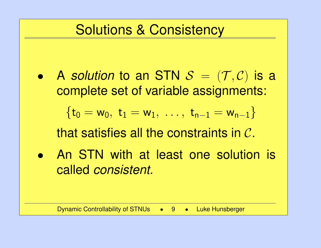
Solutions & Consistency
• A solution to an STN S = (T , C) is acomplete set of variable assignments:
t0 = w0, t1 = w1, . . . , tn−1 = wn−1that satisfies all the constraints in C.
• An STN with at least one solution iscalled consistent.
Dynamic Controllability of STNUs • 9 • Luke Hunsberger
9
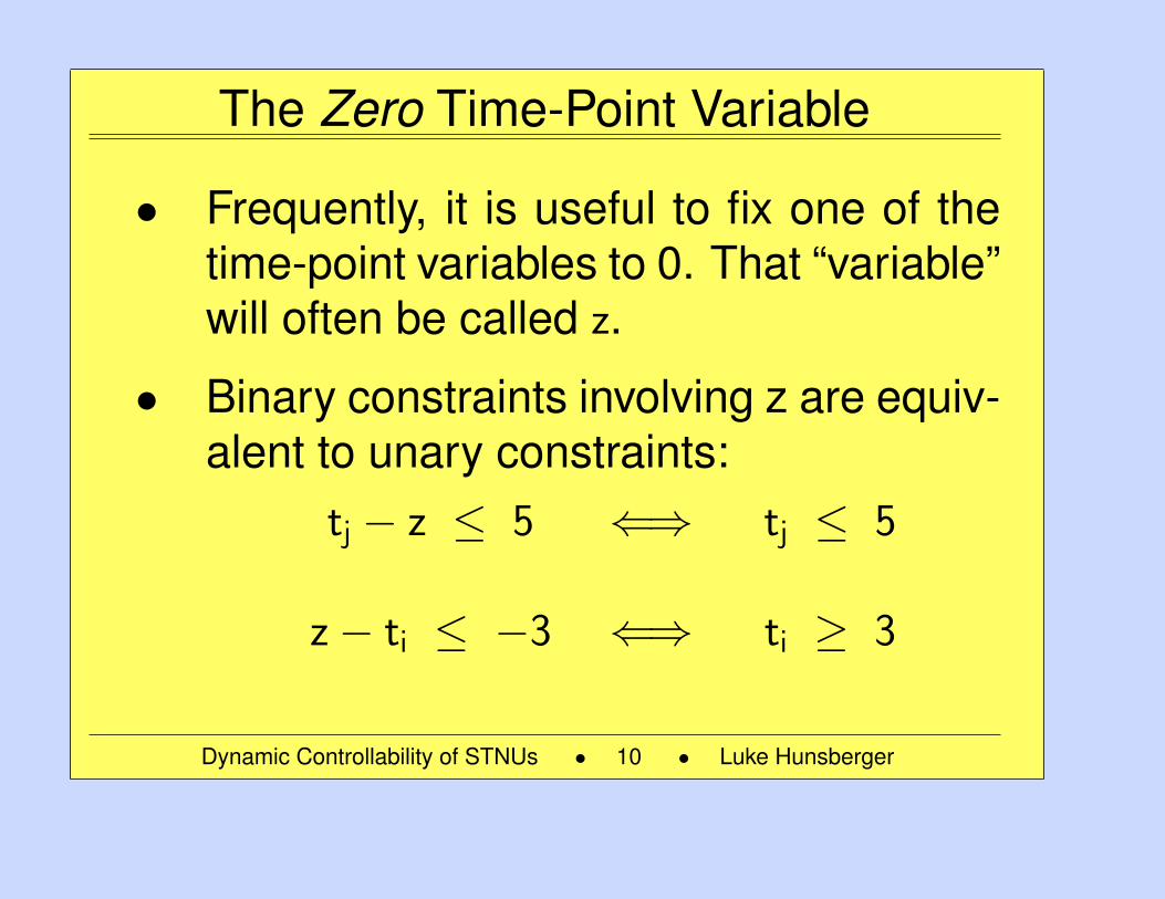
The Zero Time-Point Variable
• Frequently, it is useful to fix one of thetime-point variables to 0. That “variable”will often be called z.
• Binary constraints involving z are equiv-alent to unary constraints:
tj − z ≤ 5 ⇐⇒ tj ≤ 5
z− ti ≤ −3 ⇐⇒ ti ≥ 3
Dynamic Controllability of STNUs • 10 • Luke Hunsberger
10
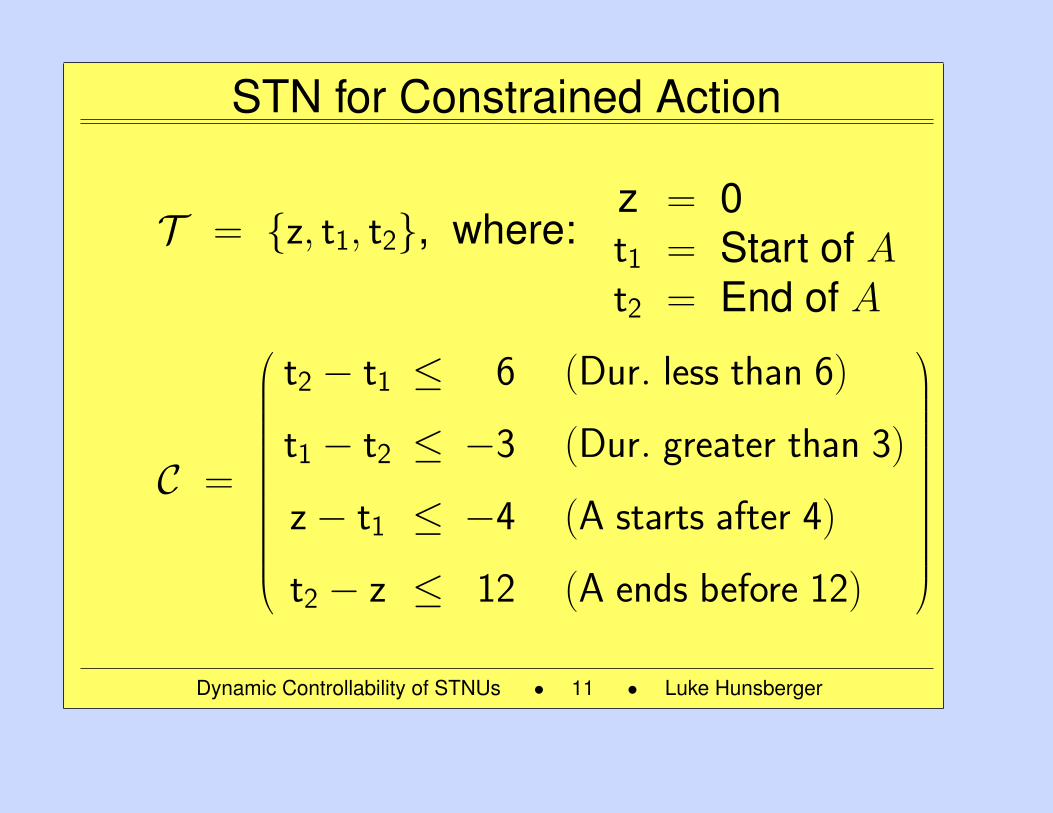
STN for Constrained Action
T = z, t1, t2, where:z = 0t1 = Start of At2 = End of A
C =
t2 − t1 ≤ 6 (Dur. less than 6)
t1 − t2 ≤ −3 (Dur. greater than 3)
z− t1 ≤ −4 (A starts after 4)
t2 − z ≤ 12 (A ends before 12)
Dynamic Controllability of STNUs • 11 • Luke Hunsberger
11
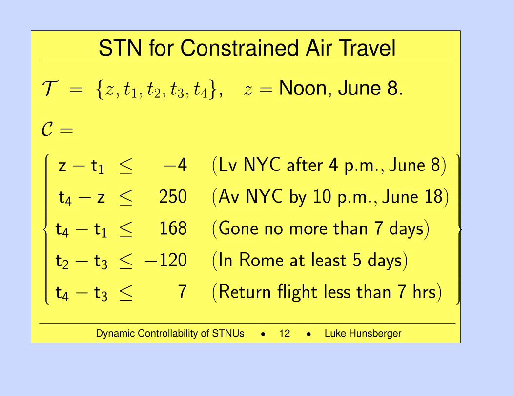
STN for Constrained Air Travel
T = z, t1, t2, t3, t4, z = Noon, June 8.
C =
z− t1 ≤ −4 (Lv NYC after 4 p.m., June 8)
t4 − z ≤ 250 (Av NYC by 10 p.m., June 18)
t4 − t1 ≤ 168 (Gone no more than 7 days)
t2 − t3 ≤ −120 (In Rome at least 5 days)
t4 − t3 ≤ 7 (Return flight less than 7 hrs)
Dynamic Controllability of STNUs • 12 • Luke Hunsberger
12
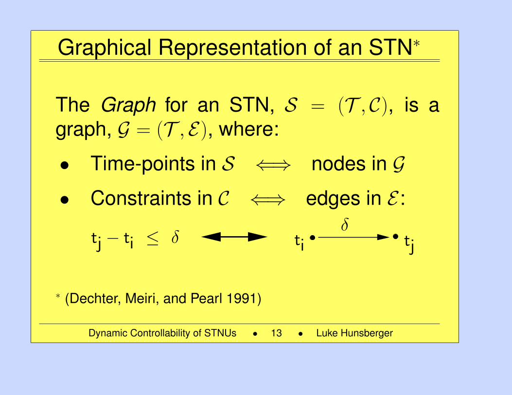
Graphical Representation of an STN∗
The Graph for an STN, S = (T , C), is agraph, G = (T , E), where:
• Time-points in S ⇐⇒ nodes in G
• Constraints in C ⇐⇒ edges in E :
tjtiδ
tj − ti ≤ δ
∗ (Dechter, Meiri, and Pearl 1991)
Dynamic Controllability of STNUs • 13 • Luke Hunsberger
13
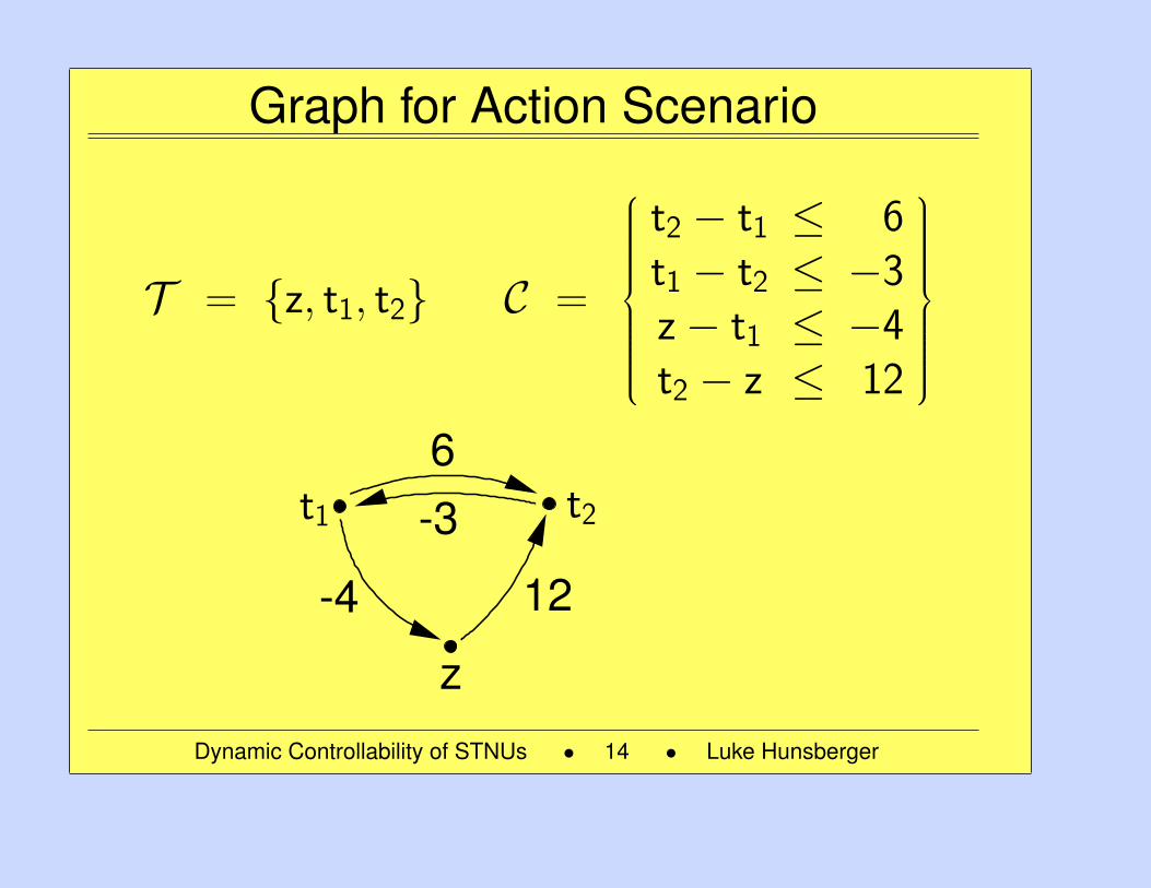
Graph for Action Scenario
T = z, t1, t2 C =
t2 − t1 ≤ 6t1 − t2 ≤ −3z− t1 ≤ −4t2 − z ≤ 12
6-3
-4 12
t1 t2
z
Dynamic Controllability of STNUs • 14 • Luke Hunsberger
14
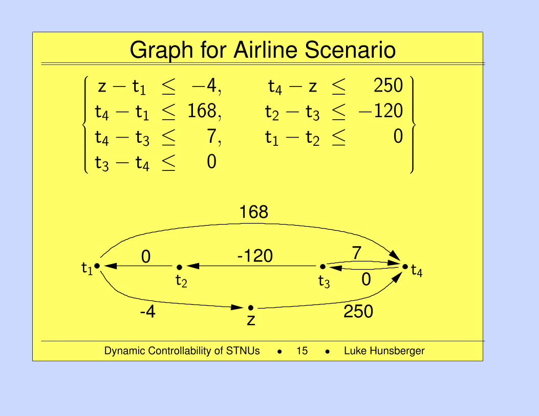
Graph for Airline Scenario
z− t1 ≤ −4, t4 − z ≤ 250t4 − t1 ≤ 168, t2 − t3 ≤ −120t4 − t3 ≤ 7, t1 − t2 ≤ 0t3 − t4 ≤ 0,
0 -120
168
07
250-4 z
t3t4t2
t1
Dynamic Controllability of STNUs • 15 • Luke Hunsberger
15
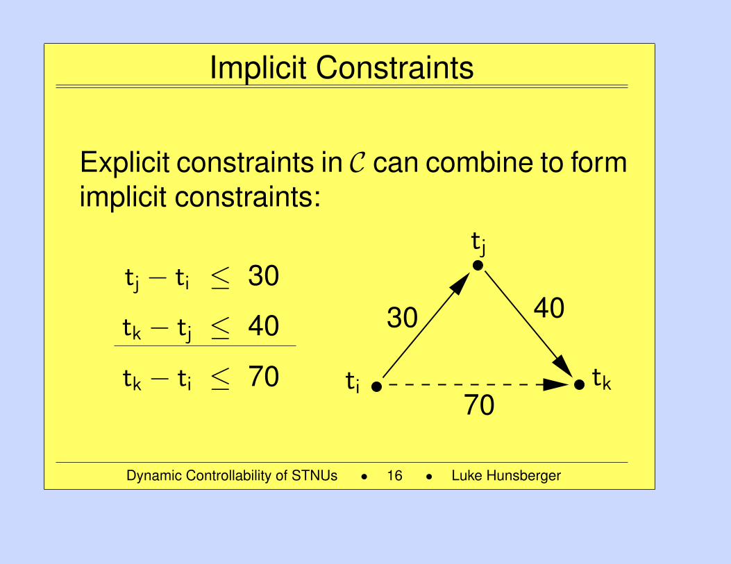
Implicit Constraints
Explicit constraints in C can combine to formimplicit constraints:
tj − ti ≤ 30
tk − tj ≤ 40
tk − ti ≤ 70
30 40
70ti tk
tj
Dynamic Controllability of STNUs • 16 • Luke Hunsberger
16
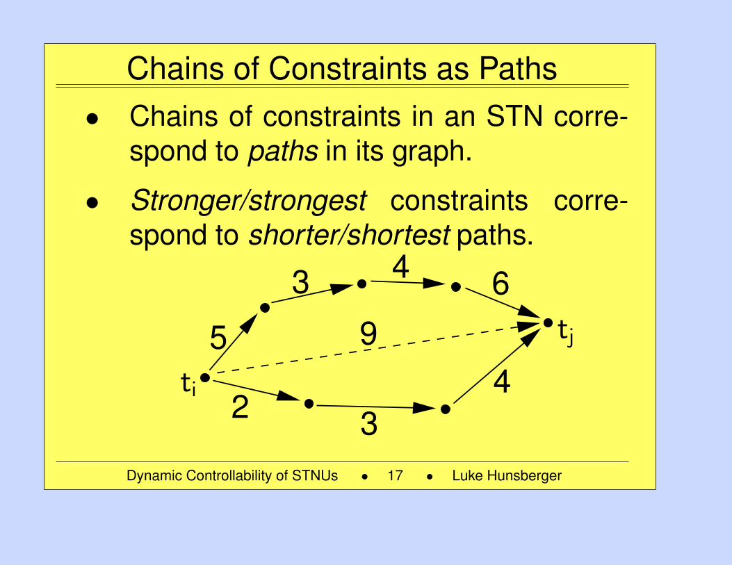
Chains of Constraints as Paths• Chains of constraints in an STN corre-
spond to paths in its graph.
• Stronger/strongest constraints corre-spond to shorter/shortest paths.
95
3 4 6
432
ti
tj
Dynamic Controllability of STNUs • 17 • Luke Hunsberger
17
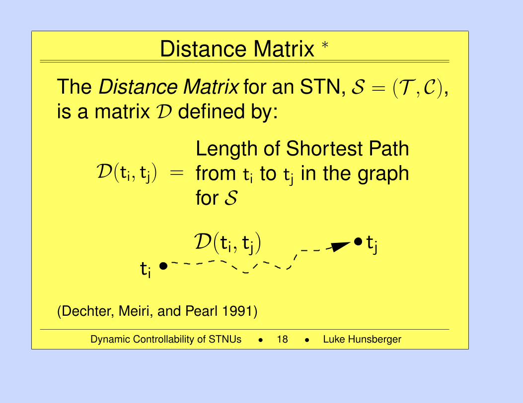
Distance Matrix ∗
The Distance Matrix for an STN, S = (T , C),is a matrix D defined by:
D(ti, tj) =Length of Shortest Pathfrom ti to tj in the graphfor S
tjti
D(ti, tj)
(Dechter, Meiri, and Pearl 1991)
Dynamic Controllability of STNUs • 18 • Luke Hunsberger
18
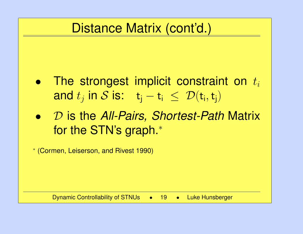
Distance Matrix (cont’d.)
• The strongest implicit constraint on tiand tj in S is: tj − ti ≤ D(ti, tj)
• D is the All-Pairs, Shortest-Path Matrixfor the STN’s graph.∗
∗ (Cormen, Leiserson, and Rivest 1990)
Dynamic Controllability of STNUs • 19 • Luke Hunsberger
19
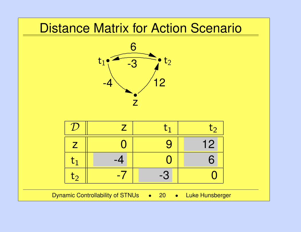
Distance Matrix for Action Scenario6-3
-4 12
t1 t2
z
D z t1 t2
z 0 9 12t1 -4 0 6t2 -7 -3 0
Dynamic Controllability of STNUs • 20 • Luke Hunsberger
20
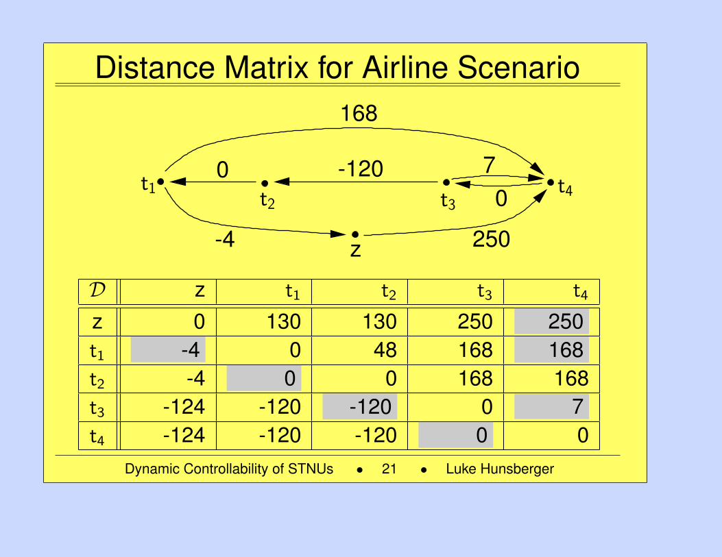
Distance Matrix for Airline Scenario
0 -120
168
07
250-4 z
t3t4t2
t1
D z t1 t2 t3 t4
z 0 130 130 250 250t1 -4 0 48 168 168t2 -4 0 0 168 168t3 -124 -120 -120 0 7t4 -124 -120 -120 0 0
Dynamic Controllability of STNUs • 21 • Luke Hunsberger
21
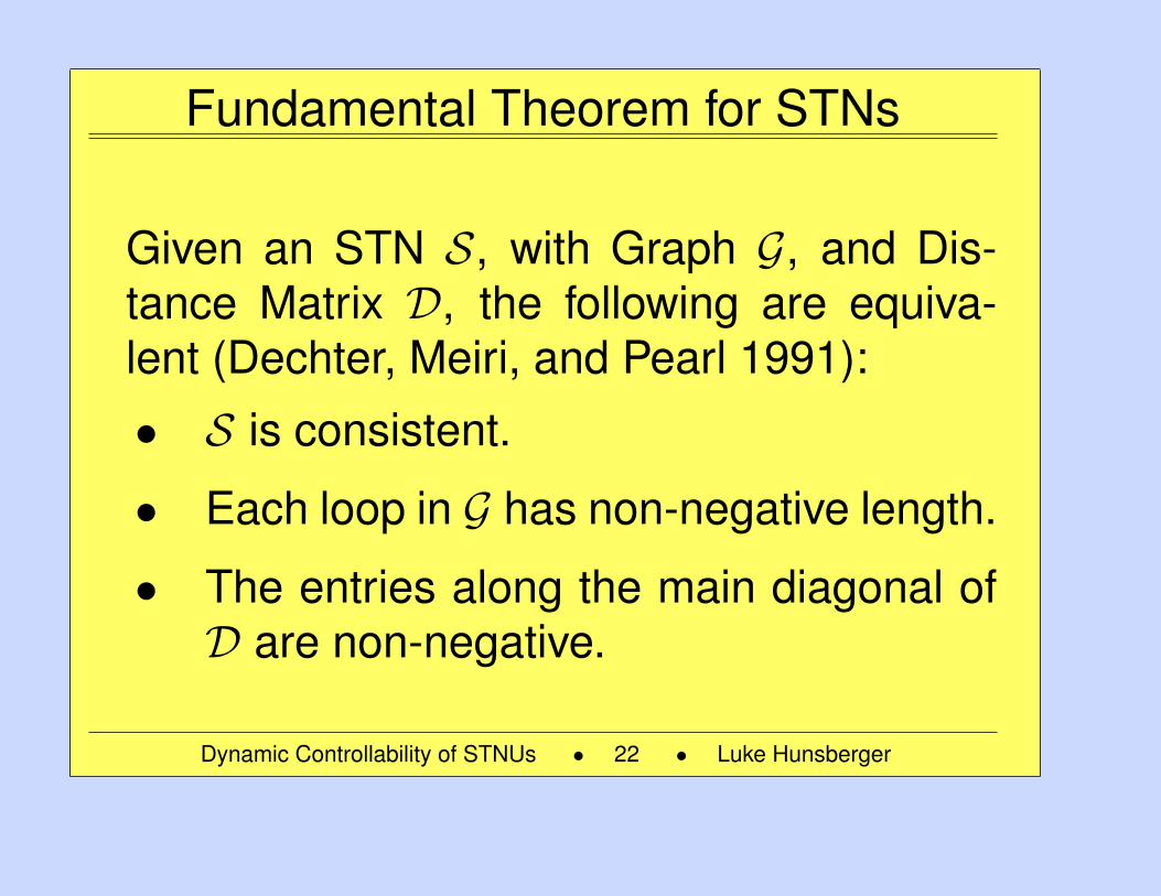
Fundamental Theorem for STNs
Given an STN S, with Graph G, and Dis-tance Matrix D, the following are equiva-lent (Dechter, Meiri, and Pearl 1991):
• S is consistent.
• Each loop in G has non-negative length.
• The entries along the main diagonal ofD are non-negative.
Dynamic Controllability of STNUs • 22 • Luke Hunsberger
22
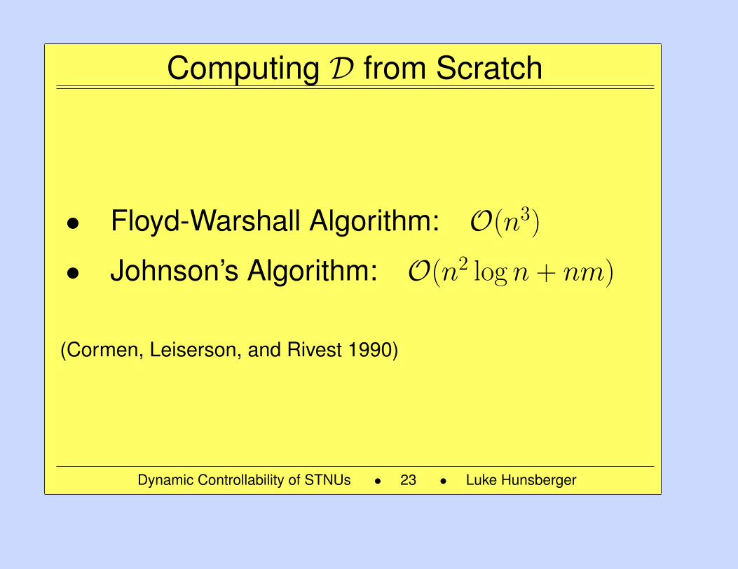
Computing D from Scratch
• Floyd-Warshall Algorithm: O(n3)
• Johnson’s Algorithm: O(n2 log n + nm)
(Cormen, Leiserson, and Rivest 1990)
Dynamic Controllability of STNUs • 23 • Luke Hunsberger
23
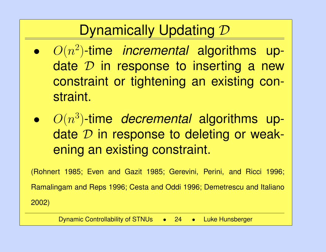
Dynamically Updating D• O(n2)-time incremental algorithms up-
date D in response to inserting a newconstraint or tightening an existing con-straint.
• O(n3)-time decremental algorithms up-date D in response to deleting or weak-ening an existing constraint.
(Rohnert 1985; Even and Gazit 1985; Gerevini, Perini, and Ricci 1996;
Ramalingam and Reps 1996; Cesta and Oddi 1996; Demetrescu and Italiano
2002)
Dynamic Controllability of STNUs • 24 • Luke Hunsberger
24
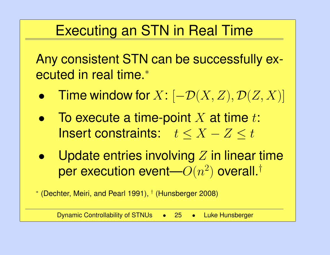
Executing an STN in Real Time
Any consistent STN can be successfully ex-ecuted in real time.∗
• Time window forX: [−D(X,Z),D(Z,X)]
• To execute a time-point X at time t:Insert constraints: t ≤ X − Z ≤ t
• Update entries involving Z in linear timeper execution event—O(n2) overall.†
∗ (Dechter, Meiri, and Pearl 1991), † (Hunsberger 2008)
Dynamic Controllability of STNUs • 25 • Luke Hunsberger
25
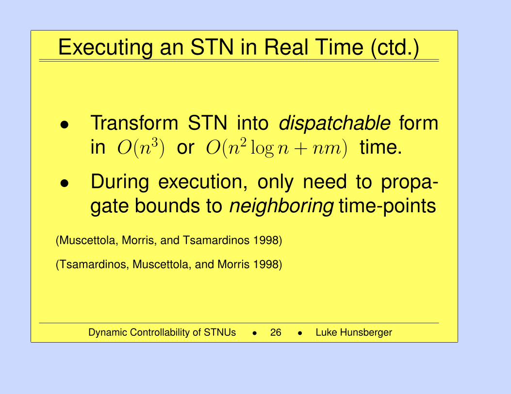
Executing an STN in Real Time (ctd.)
• Transform STN into dispatchable formin O(n3) or O(n2 log n + nm) time.
• During execution, only need to propa-gate bounds to neighboring time-points
(Muscettola, Morris, and Tsamardinos 1998)
(Tsamardinos, Muscettola, and Morris 1998)
Dynamic Controllability of STNUs • 26 • Luke Hunsberger
26
STNs with Uncertainty
Dynamic Controllability of STNUs • 27 • Luke Hunsberger
27
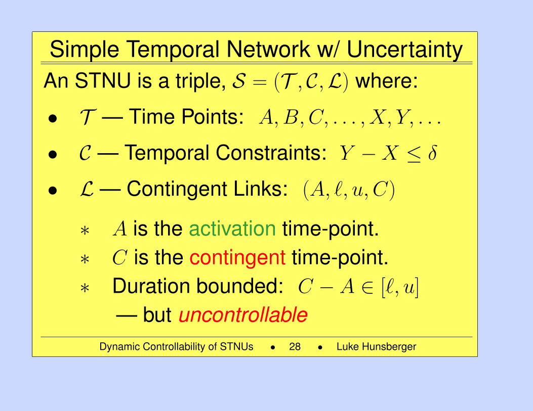
Simple Temporal Network w/ UncertaintyAn STNU is a triple, S = (T , C,L) where:
• T — Time Points: A,B,C, . . . , X, Y, . . .
• C — Temporal Constraints: Y −X ≤ δ
• L— Contingent Links: (A, `, u, C)
∗ A is the activation time-point.∗ C is the contingent time-point.∗ Duration bounded: C − A ∈ [`, u]
— but uncontrollableDynamic Controllability of STNUs • 28 • Luke Hunsberger
28
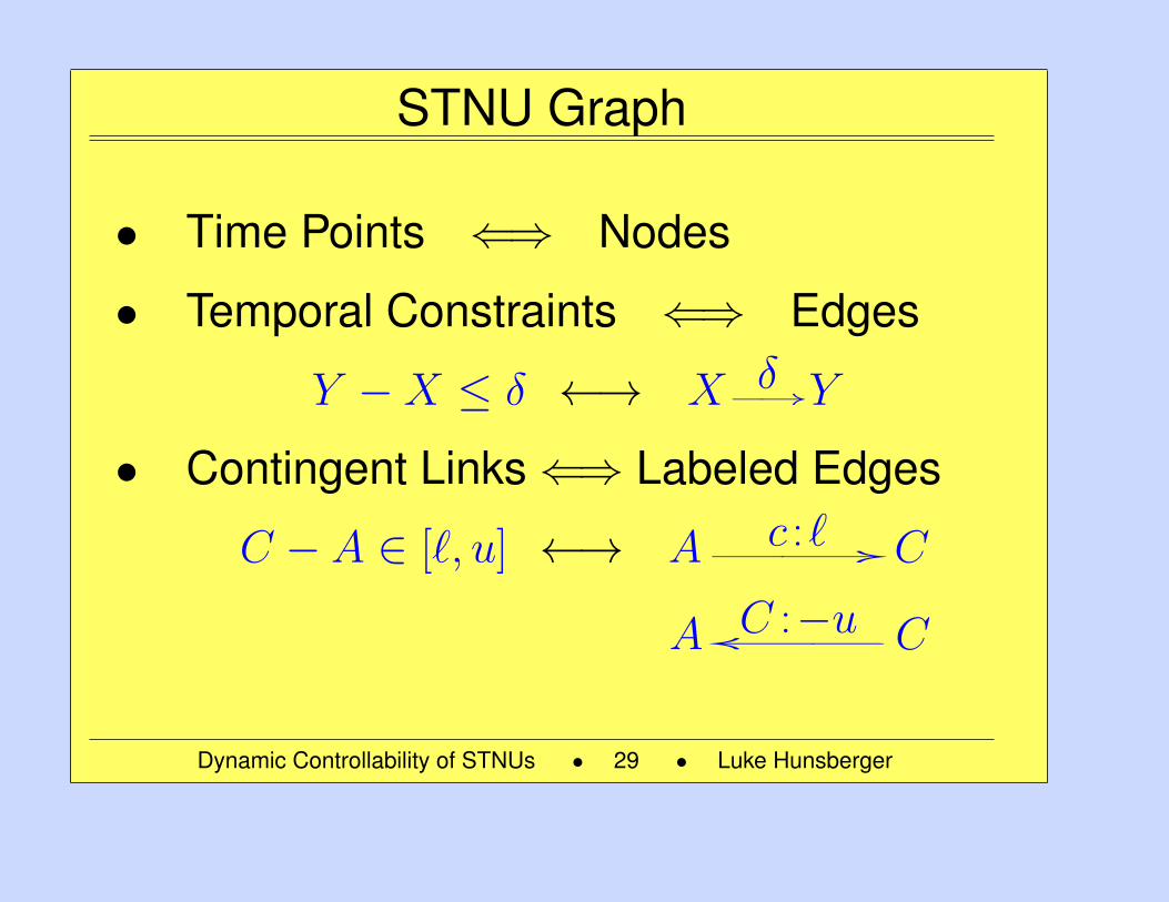
STNU Graph
• Time Points ⇐⇒ Nodes
• Temporal Constraints ⇐⇒ Edges
Y −X ≤ δ ←→ X−→δ Y
• Contingent Links⇐⇒ Labeled Edges
C − A ∈ [`, u] ←→ A−→c :` C
A←−C :−u C
Dynamic Controllability of STNUs • 29 • Luke Hunsberger
29
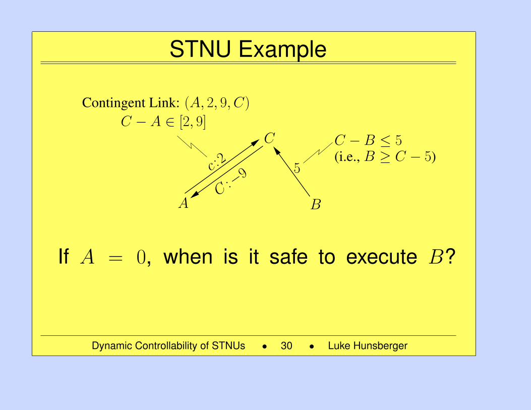
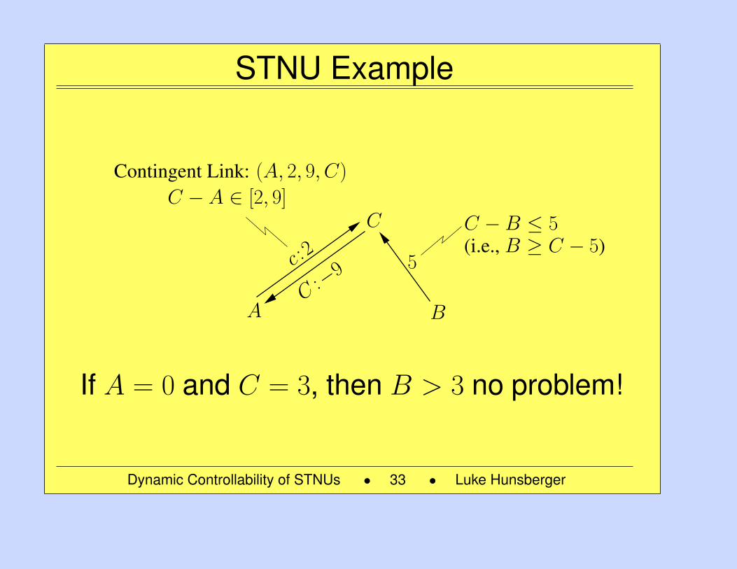
STNU Example
Contingent Link: (A, 2, 9, C)
C
B
5c :2
C:−9
C − A ∈ [2, 9]
C −B ≤ 5(i.e., B ≥ C − 5)
A
If A = 0, when is it safe to execute B?
Dynamic Controllability of STNUs • 30 • Luke Hunsberger
30
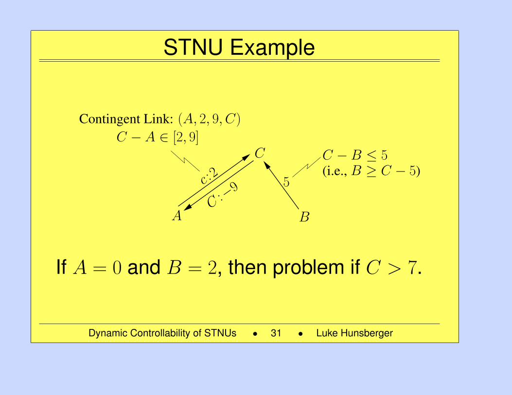
STNU Example
Contingent Link: (A, 2, 9, C)
C
B
5c :2
C:−9
C − A ∈ [2, 9]
C −B ≤ 5(i.e., B ≥ C − 5)
A
If A = 0 and B = 2, then problem if C > 7.
Dynamic Controllability of STNUs • 31 • Luke Hunsberger
31
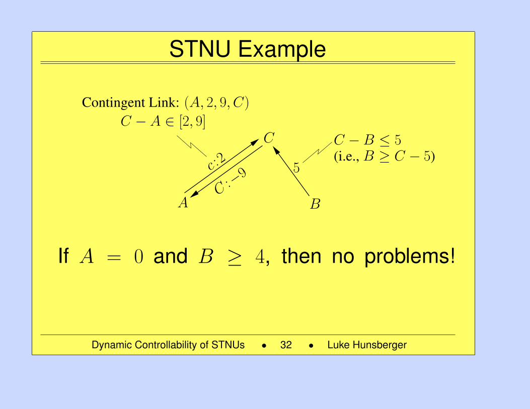
STNU Example
Contingent Link: (A, 2, 9, C)
C
B
5c :2
C:−9
C − A ∈ [2, 9]
C −B ≤ 5(i.e., B ≥ C − 5)
A
If A = 0 and B ≥ 4, then no problems!
Dynamic Controllability of STNUs • 32 • Luke Hunsberger
32
STNU Example
Contingent Link: (A, 2, 9, C)
C
B
5c :2
C:−9
C − A ∈ [2, 9]
C −B ≤ 5(i.e., B ≥ C − 5)
A
If A = 0 and C = 3, then B > 3 no problem!
Dynamic Controllability of STNUs • 33 • Luke Hunsberger
33
Dynamic Controllability (DC)
An STNU is dynamically controllable if thereexists a strategy for executing the non-contingent time-points such that all of theconstraints in the network will be satisfied—no matter how the durations of the contin-gent links turn out.
Dynamic Controllability of STNUs • 34 • Luke Hunsberger
34
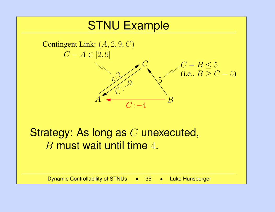
STNU Example
C :−4
C
B
5c :2
C:−9
C − A ∈ [2, 9]
C −B ≤ 5(i.e., B ≥ C − 5)
A
Contingent Link: (A, 2, 9, C)
Strategy: As long as C unexecuted,B must wait until time 4.
Dynamic Controllability of STNUs • 35 • Luke Hunsberger
35
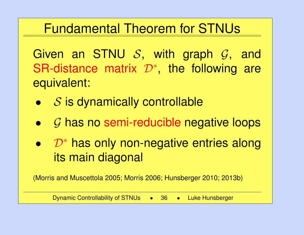
Fundamental Theorem for STNUs
Given an STNU S, with graph G, andSR-distance matrix D∗, the following areequivalent:
• S is dynamically controllable
• G has no semi-reducible negative loops
• D∗ has only non-negative entries alongits main diagonal
(Morris and Muscettola 2005; Morris 2006; Hunsberger 2010; 2013b)
Dynamic Controllability of STNUs • 36 • Luke Hunsberger
36
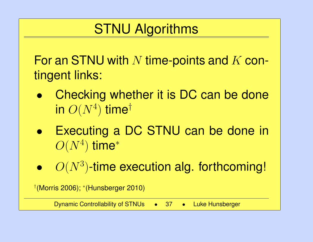
STNU Algorithms
For an STNU withN time-points andK con-tingent links:
• Checking whether it is DC can be donein O(N 4) time†
• Executing a DC STNU can be done inO(N 4) time∗
• O(N 3)-time execution alg. forthcoming!†(Morris 2006); ∗(Hunsberger 2010)
Dynamic Controllability of STNUs • 37 • Luke Hunsberger
37
Dynamic Controllability (DC)
Dynamic Controllability of STNUs • 38 • Luke Hunsberger
38
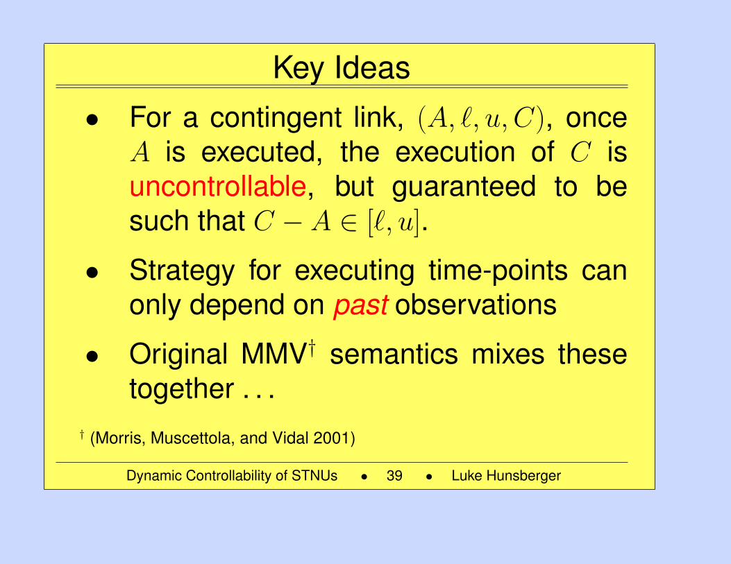
Key Ideas• For a contingent link, (A, `, u, C), once
A is executed, the execution of C isuncontrollable, but guaranteed to besuch that C − A ∈ [`, u].
• Strategy for executing time-points canonly depend on past observations
• Original MMV† semantics mixes thesetogether . . .
† (Morris, Muscettola, and Vidal 2001)
Dynamic Controllability of STNUs • 39 • Luke Hunsberger
39
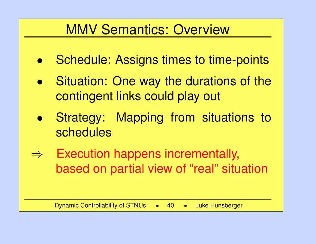
MMV Semantics: Overview
• Schedule: Assigns times to time-points
• Situation: One way the durations of thecontingent links could play out
• Strategy: Mapping from situations toschedules
⇒ Execution happens incrementally,based on partial view of “real” situation
Dynamic Controllability of STNUs • 40 • Luke Hunsberger
40
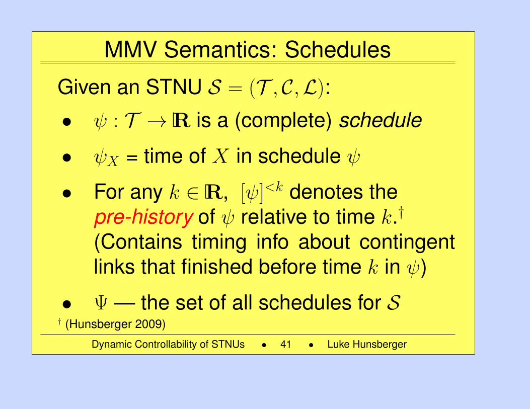
MMV Semantics: Schedules
Given an STNU S = (T , C,L):
• ψ : T → R is a (complete) schedule
• ψX = time of X in schedule ψ
• For any k ∈ R, [ψ]<k denotes thepre-history of ψ relative to time k.†
(Contains timing info about contingentlinks that finished before time k in ψ)
• Ψ — the set of all schedules for S† (Hunsberger 2009)
Dynamic Controllability of STNUs • 41 • Luke Hunsberger
41
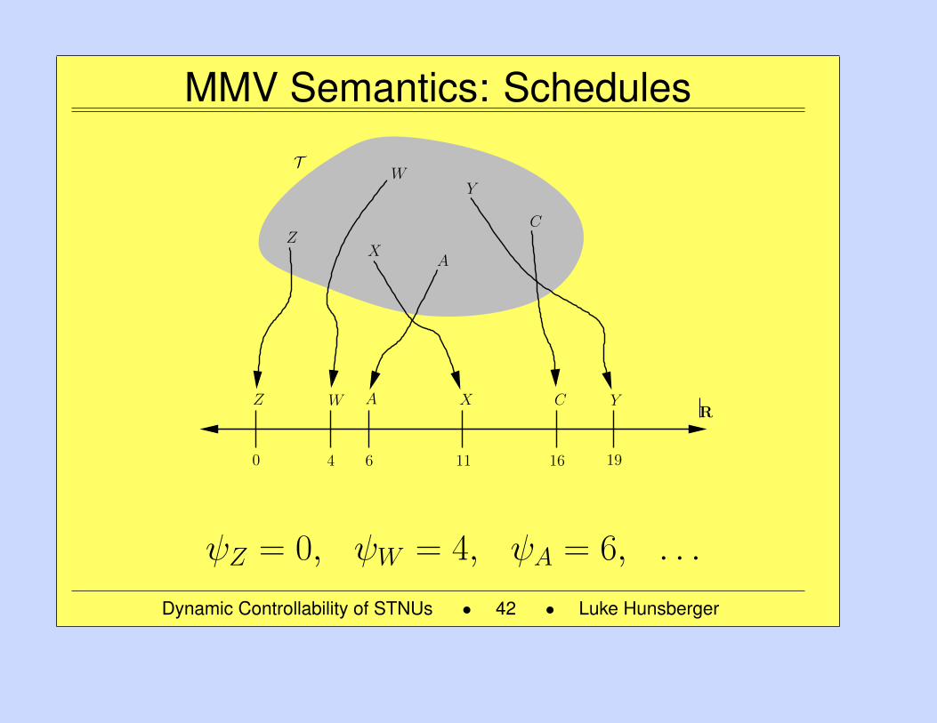
MMV Semantics: Schedules
RW A X C Y
0 4 6 11 16 19
Z
WY
X
T
A
C
Z
ψZ = 0, ψW = 4, ψA = 6, . . .
Dynamic Controllability of STNUs • 42 • Luke Hunsberger
42
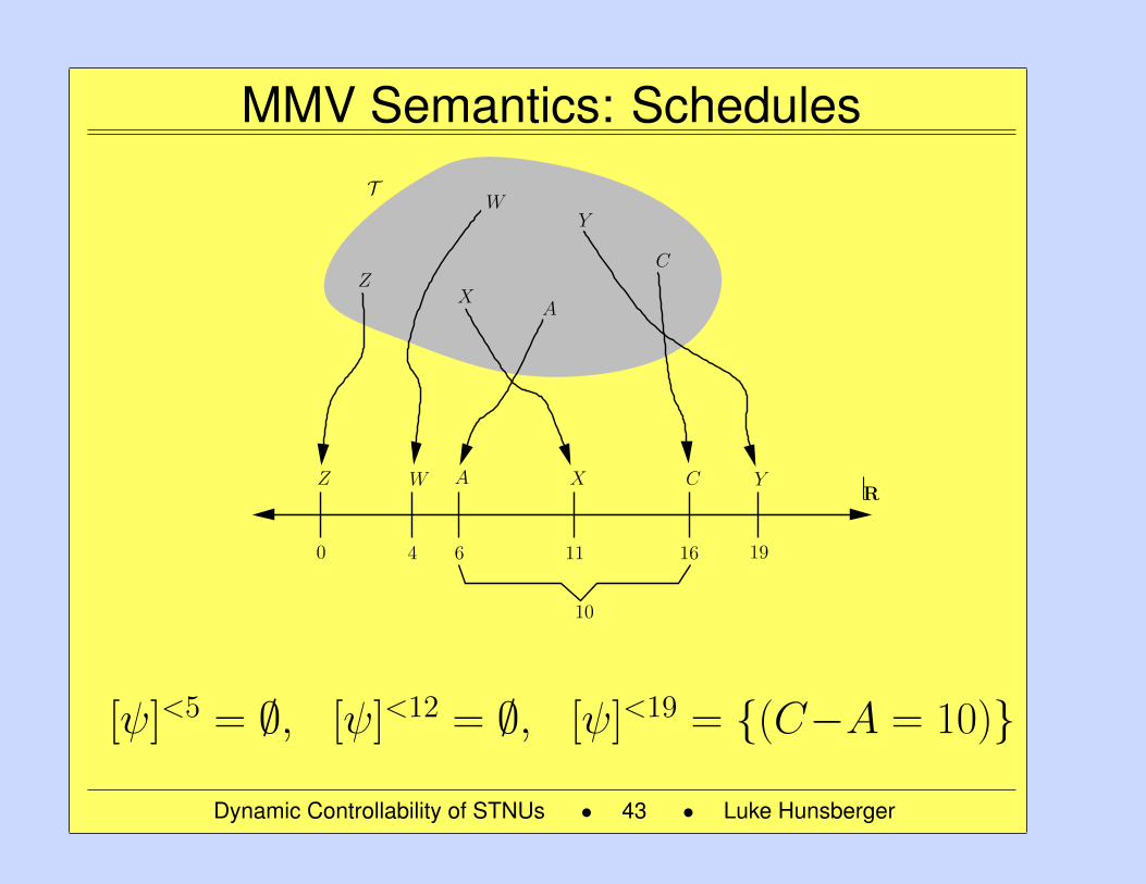
MMV Semantics: Schedules
RZ W A X C Y
0 4 6 11 16 19
Z
WY
X
T
A
C
10
[ψ]<5 = ∅, [ψ]<12 = ∅, [ψ]<19 = (C−A = 10)
Dynamic Controllability of STNUs • 43 • Luke Hunsberger
43
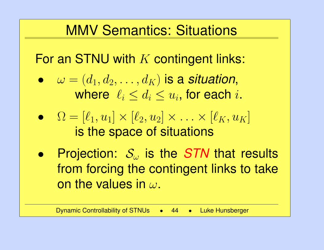
MMV Semantics: Situations
For an STNU with K contingent links:
• ω = (d1, d2, . . . , dK) is a situation,where `i ≤ di ≤ ui, for each i.
• Ω = [`1, u1]× [`2, u2]× . . .× [`K, uK]is the space of situations
• Projection: Sω is the STN that resultsfrom forcing the contingent links to takeon the values in ω.
Dynamic Controllability of STNUs • 44 • Luke Hunsberger
44
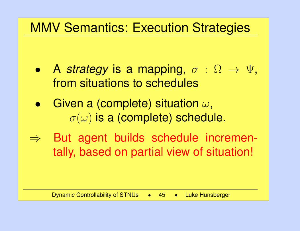
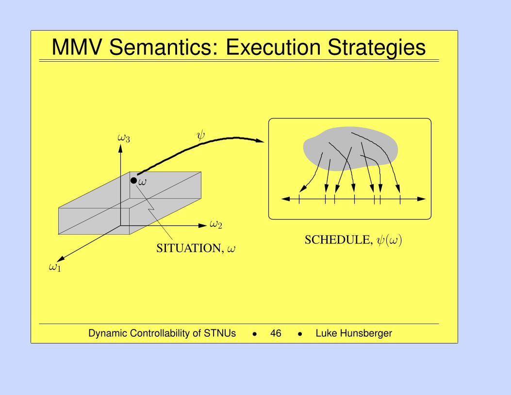
MMV Semantics: Execution Strategies
• A strategy is a mapping, σ : Ω → Ψ,from situations to schedules
• Given a (complete) situation ω,σ(ω) is a (complete) schedule.
⇒ But agent builds schedule incremen-tally, based on partial view of situation!
Dynamic Controllability of STNUs • 45 • Luke Hunsberger
45
MMV Semantics: Execution Strategies
SCHEDULE, ψ(ω)SITUATION, ω
ψ
ω1
ω2
ω
ω3
Dynamic Controllability of STNUs • 46 • Luke Hunsberger
46
MMV Semantics: Valid Strategies
• A strategy σ is valid if for each situation ω,the schedule σ(ω) is consistent with theprojection Sω.
⇒ In other words, a valid strategy does notcontrol the durations of contingent links.
Dynamic Controllability of STNUs • 47 • Luke Hunsberger
47
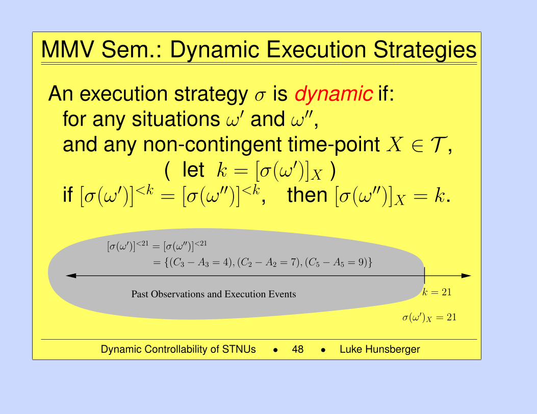
MMV Sem.: Dynamic Execution Strategies
An execution strategy σ is dynamic if:for any situations ω′ and ω′′,and any non-contingent time-point X ∈ T ,
( let k = [σ(ω′)]X )if [σ(ω′)]<k = [σ(ω′′)]<k, then [σ(ω′′)]X = k.
σ(ω′)X = 21
Past Observations and Execution Events
[σ(ω′)]<21 = [σ(ω′′)]<21
= (C3 − A3 = 4), (C2 − A2 = 7), (C5 − A5 = 9)
k = 21
Dynamic Controllability of STNUs • 48 • Luke Hunsberger
48
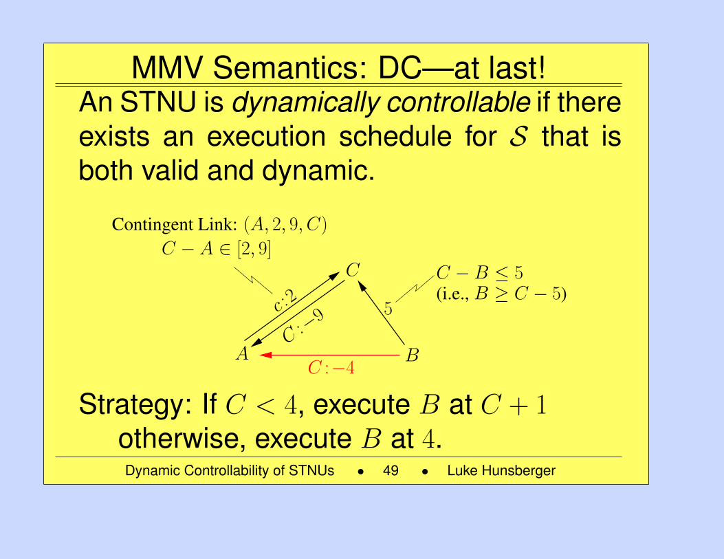
MMV Semantics: DC—at last!An STNU is dynamically controllable if thereexists an execution schedule for S that isboth valid and dynamic.
C :−4
C
B
5c :2
C:−9
C − A ∈ [2, 9]
C −B ≤ 5(i.e., B ≥ C − 5)
A
Contingent Link: (A, 2, 9, C)
Strategy: If C < 4, execute B at C + 1otherwise, execute B at 4.Dynamic Controllability of STNUs • 49 • Luke Hunsberger
49
Alternative Semantics• Real-time execution decisions (RTEDs)
based on partial situations
• Makes explicit the decision problemfaced during execution
• Outcomes of RTEDs reflect all possiblesituations
• Equivalent to MMV semantics
(Hunsberger 2009)
Dynamic Controllability of STNUs • 50 • Luke Hunsberger
50
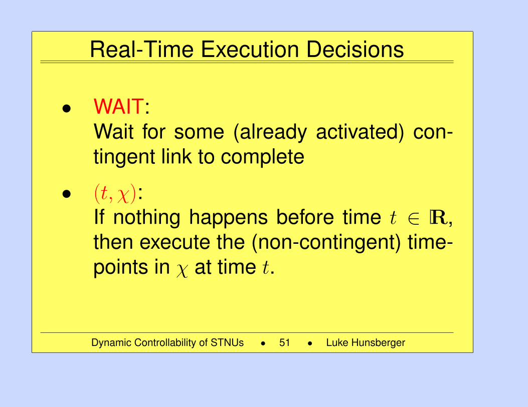
Real-Time Execution Decisions
• WAIT:Wait for some (already activated) con-tingent link to complete
• (t, χ):If nothing happens before time t ∈ R,then execute the (non-contingent) time-points in χ at time t.
Dynamic Controllability of STNUs • 51 • Luke Hunsberger
51
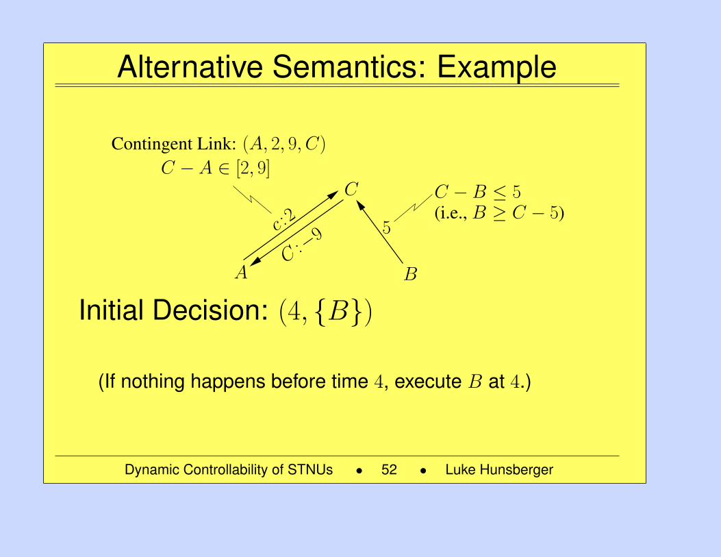
Alternative Semantics: Example
Contingent Link: (A, 2, 9, C)
C
B
5c :2
C:−9
C − A ∈ [2, 9]
C −B ≤ 5(i.e., B ≥ C − 5)
A
Initial Decision: (4, B)
(If nothing happens before time 4, execute B at 4.)
Dynamic Controllability of STNUs • 52 • Luke Hunsberger
52
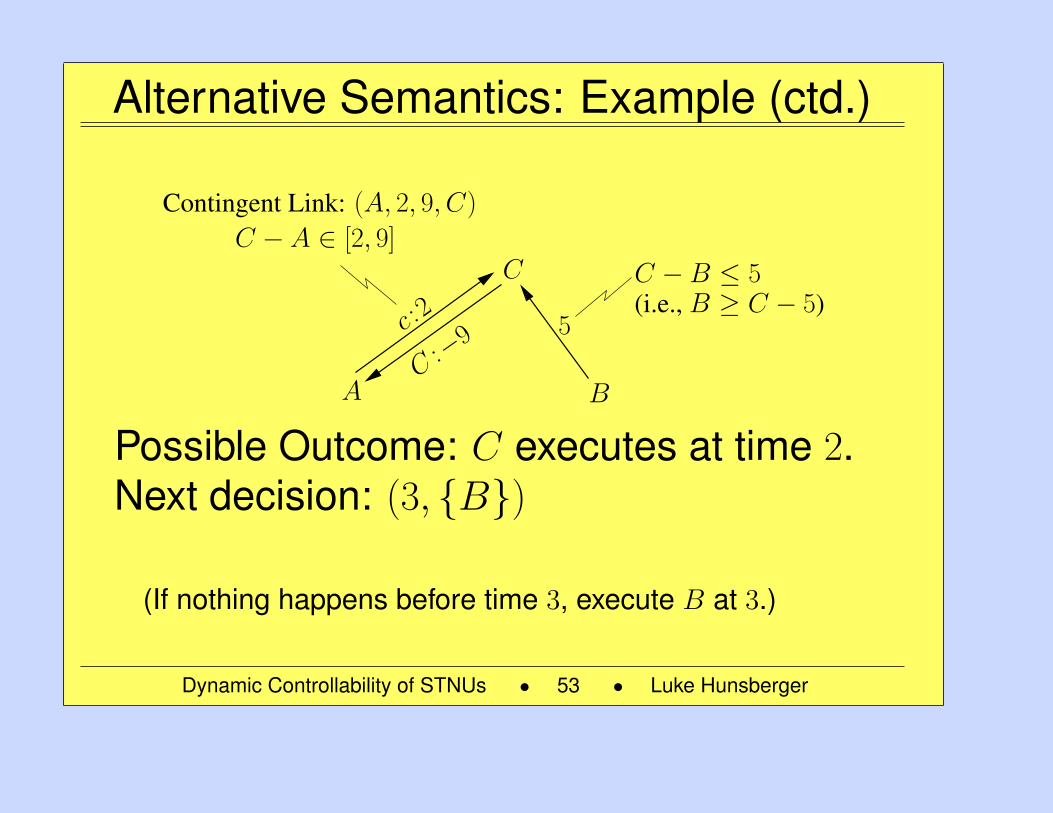
Alternative Semantics: Example (ctd.)
Contingent Link: (A, 2, 9, C)
C
B
5c :2
C:−9
C − A ∈ [2, 9]
C −B ≤ 5(i.e., B ≥ C − 5)
A
Possible Outcome: C executes at time 2.Next decision: (3, B)
(If nothing happens before time 3, execute B at 3.)
Dynamic Controllability of STNUs • 53 • Luke Hunsberger
53
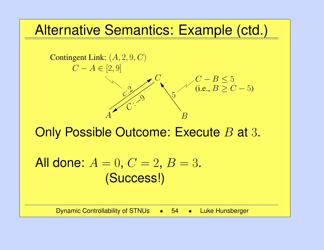
Alternative Semantics: Example (ctd.)
Contingent Link: (A, 2, 9, C)
C
B
5c :2
C:−9
C − A ∈ [2, 9]
C −B ≤ 5(i.e., B ≥ C − 5)
A
Only Possible Outcome: Execute B at 3.
All done: A = 0, C = 2, B = 3.(Success!)
Dynamic Controllability of STNUs • 54 • Luke Hunsberger
54
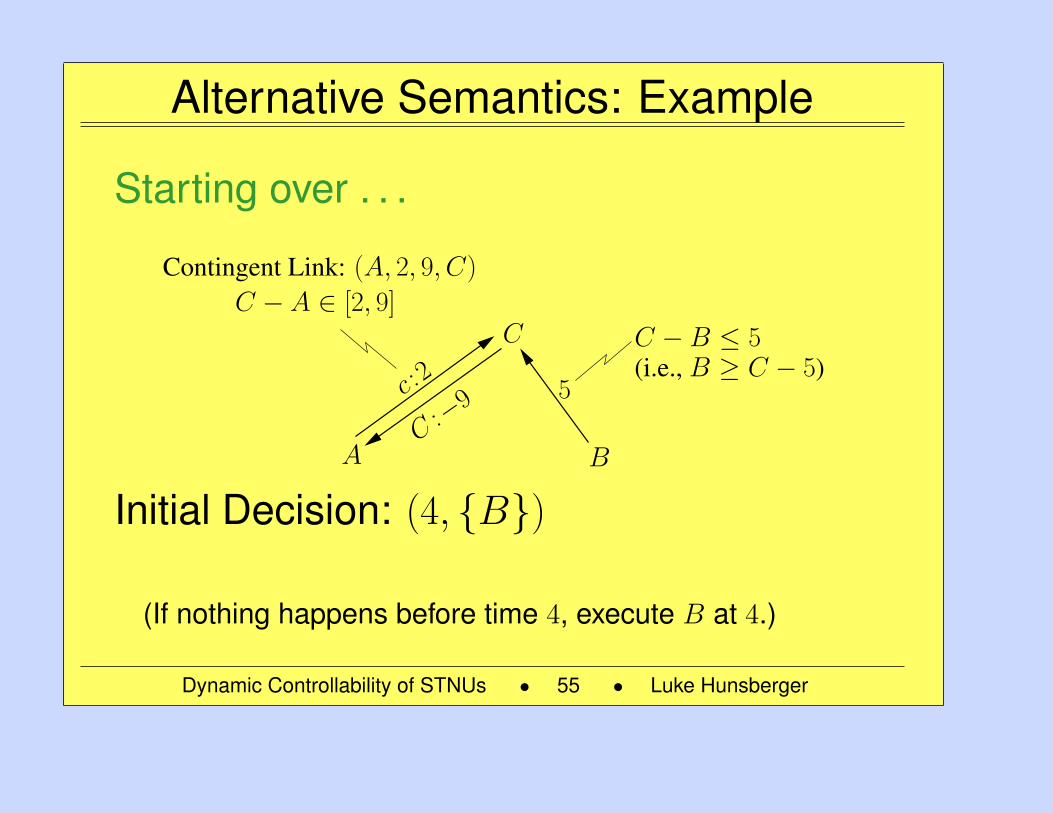
Alternative Semantics: Example
Starting over . . .
Contingent Link: (A, 2, 9, C)
C
B
5c :2
C:−9
C − A ∈ [2, 9]
C −B ≤ 5(i.e., B ≥ C − 5)
A
Initial Decision: (4, B)
(If nothing happens before time 4, execute B at 4.)
Dynamic Controllability of STNUs • 55 • Luke Hunsberger
55
Alternative Semantics: Example (ctd.)
Contingent Link: (A, 2, 9, C)
C
B
5c :2
C:−9
C − A ∈ [2, 9]
C −B ≤ 5(i.e., B ≥ C − 5)
A
Possible Outcome: C does not execute yet;so B executed at 4
Next decision: WAIT (for C to execute)
Dynamic Controllability of STNUs • 56 • Luke Hunsberger
56
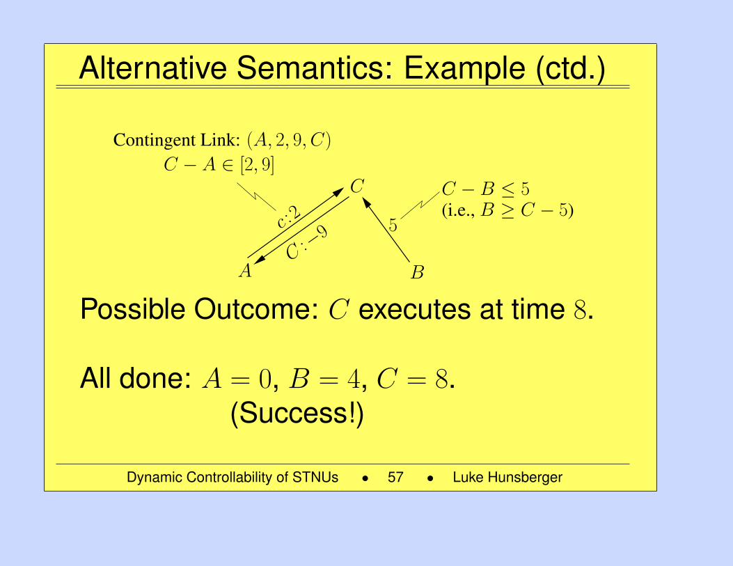
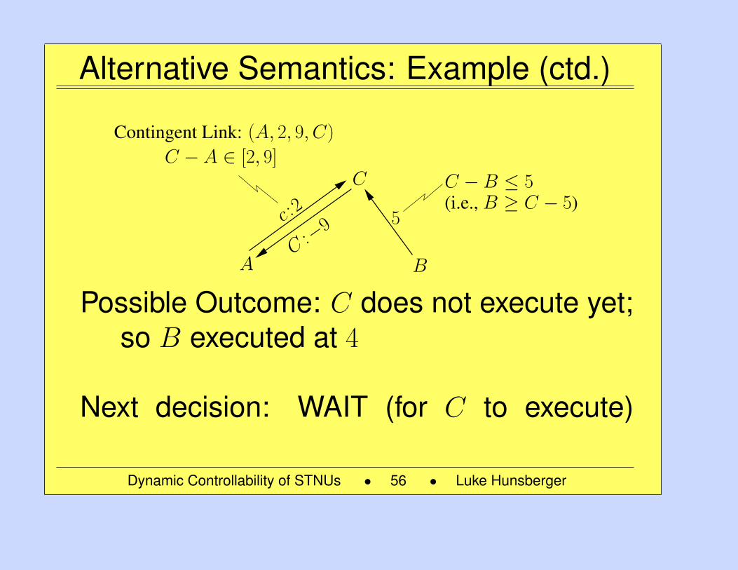
Alternative Semantics: Example (ctd.)
Contingent Link: (A, 2, 9, C)
C
B
5c :2
C:−9
C − A ∈ [2, 9]
C −B ≤ 5(i.e., B ≥ C − 5)
A
Possible Outcome: C executes at time 8.
All done: A = 0, B = 4, C = 8.(Success!)
Dynamic Controllability of STNUs • 57 • Luke Hunsberger
57
Two Formulations Equivalent
• There is a one-to-one correspondencebetween dynamic execution strate-gies (Morris, Muscettola, and Vidal 2001) andstrategies based on real-time executiondecisions (Hunsberger 2009)
• RTED-based strategies more practicalfor agents executing an STNU in realtime
Dynamic Controllability of STNUs • 58 • Luke Hunsberger
58
DC-Checking Algorithms
Dynamic Controllability of STNUs • 59 • Luke Hunsberger
59
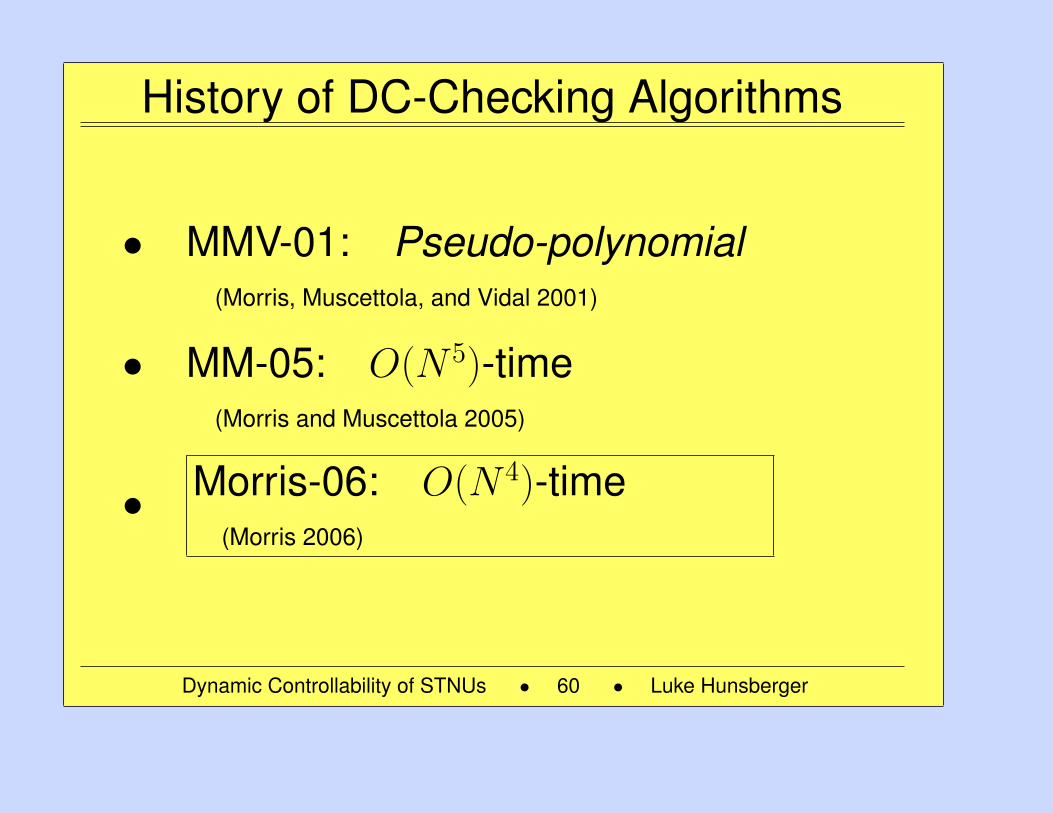
History of DC-Checking Algorithms
• MMV-01: Pseudo-polynomial(Morris, Muscettola, and Vidal 2001)
• MM-05: O(N 5)-time(Morris and Muscettola 2005)
• Morris-06: O(N 4)-time(Morris 2006)
Dynamic Controllability of STNUs • 60 • Luke Hunsberger
60
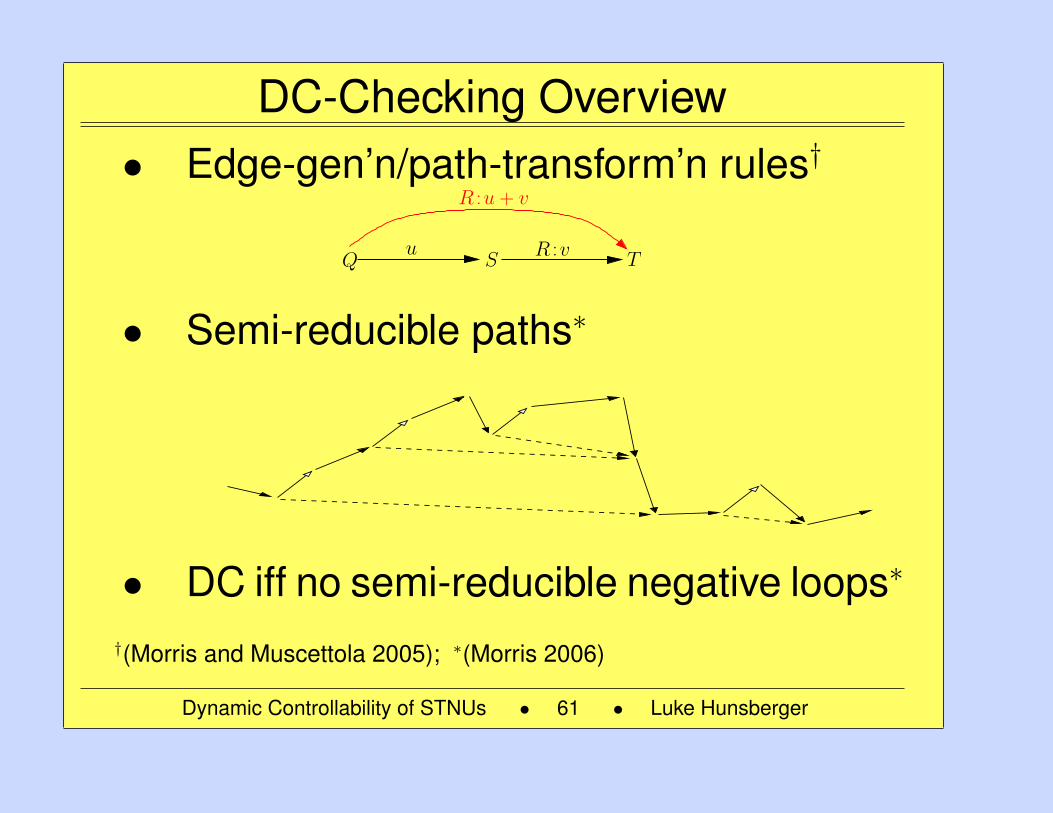
DC-Checking Overview• Edge-gen’n/path-transform’n rules†
R :u + v
Q S Tu R :v
• Semi-reducible paths∗
• DC iff no semi-reducible negative loops∗
†(Morris and Muscettola 2005); ∗(Morris 2006)
Dynamic Controllability of STNUs • 61 • Luke Hunsberger
61
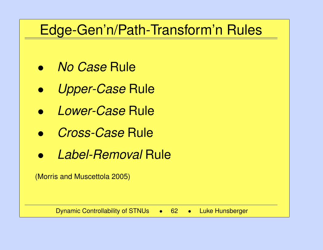
Edge-Gen’n/Path-Transform’n Rules
• No Case Rule
• Upper-Case Rule
• Lower-Case Rule
• Cross-Case Rule
• Label-Removal Rule
(Morris and Muscettola 2005)
Dynamic Controllability of STNUs • 62 • Luke Hunsberger
62
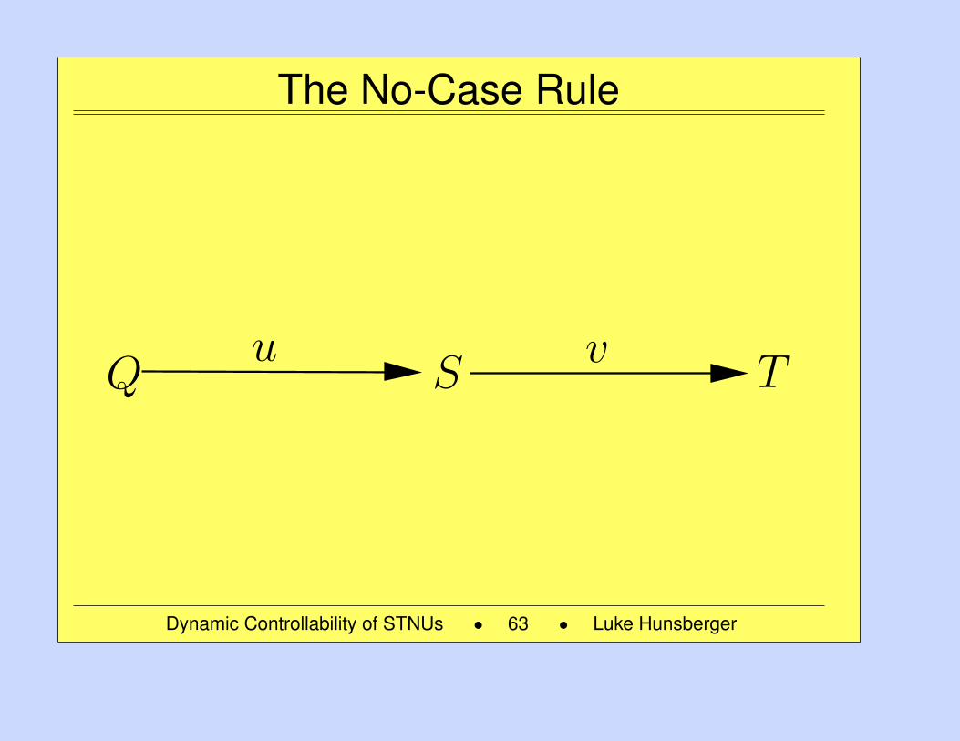
The No-Case Rule
Q S Tu v
Dynamic Controllability of STNUs • 63 • Luke Hunsberger
63
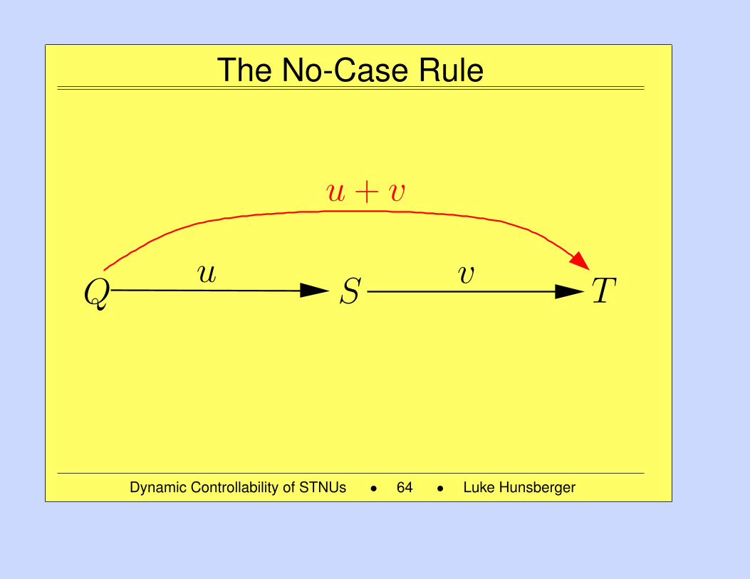
The No-Case Rule
u + v
Q S Tu v
Dynamic Controllability of STNUs • 64 • Luke Hunsberger
64
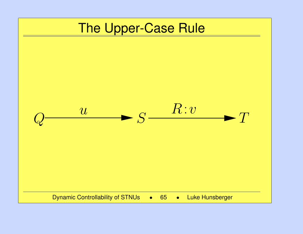
The Upper-Case Rule
Q S Tu R :v
Dynamic Controllability of STNUs • 65 • Luke Hunsberger
65
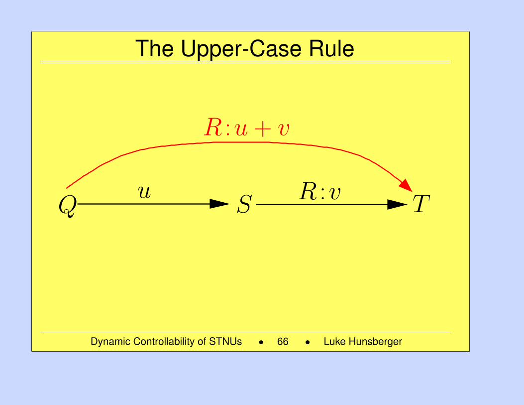
The Upper-Case Rule
R :u + v
Q S Tu R :v
Dynamic Controllability of STNUs • 66 • Luke Hunsberger
66
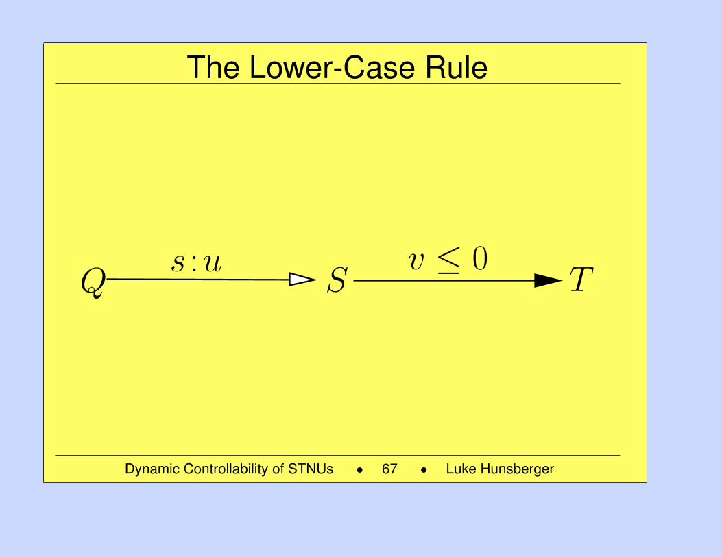
The Lower-Case Rule
Q S Ts :u v ≤ 0
Dynamic Controllability of STNUs • 67 • Luke Hunsberger
67
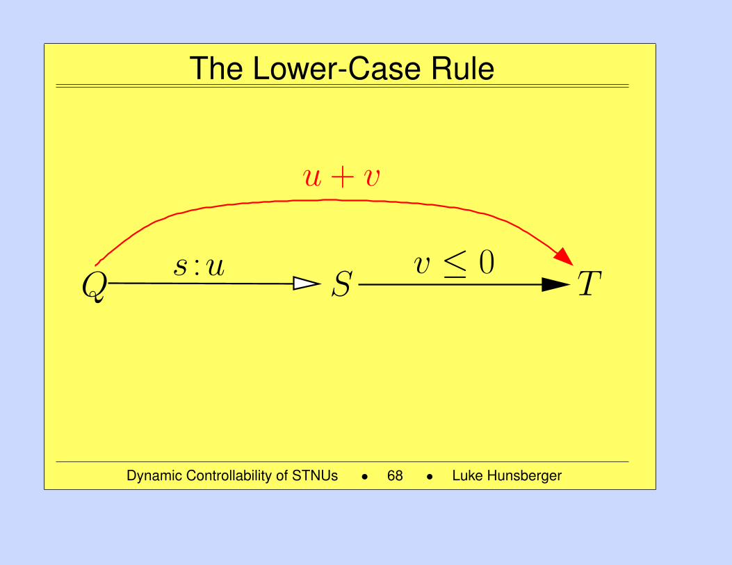
The Lower-Case Rule
u + v
Q S Ts :u v ≤ 0
Dynamic Controllability of STNUs • 68 • Luke Hunsberger
68
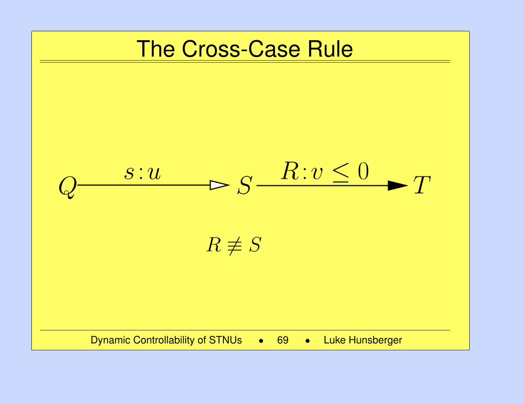
The Cross-Case Rule
Q S Ts :u R :v ≤ 0
R 6≡ S
Dynamic Controllability of STNUs • 69 • Luke Hunsberger
69
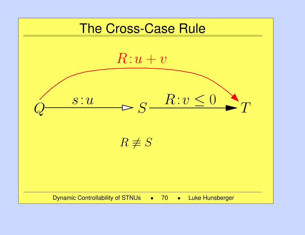
The Cross-Case Rule
R :u + v
Q S Ts :u R :v ≤ 0
R 6≡ S
Dynamic Controllability of STNUs • 70 • Luke Hunsberger
70
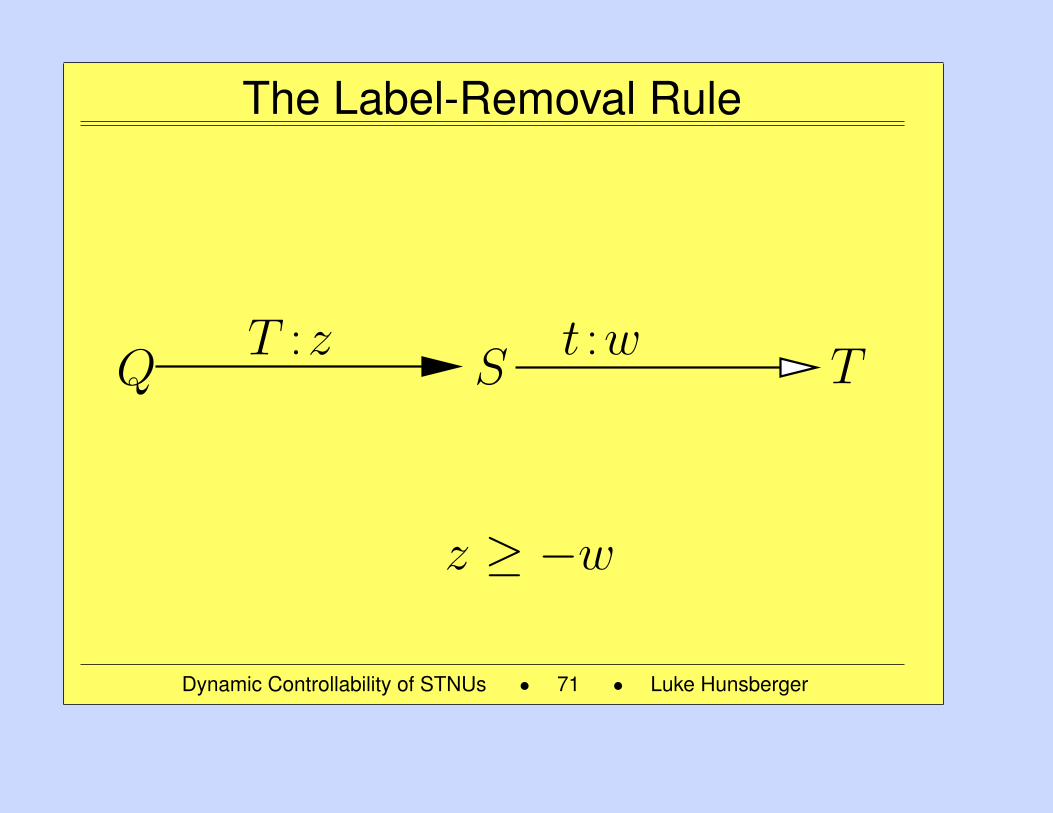
The Label-Removal Rule
Q S TT :z t :w
z ≥ −w
Dynamic Controllability of STNUs • 71 • Luke Hunsberger
71
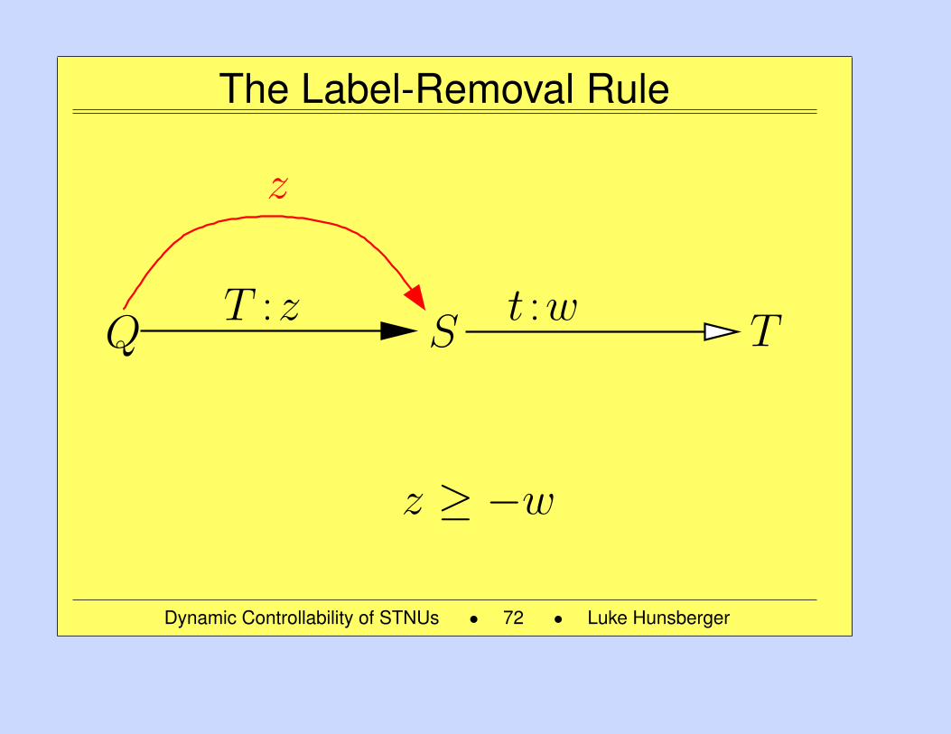
The Label-Removal Rule
z
Q S TT :z t :w
z ≥ −w
Dynamic Controllability of STNUs • 72 • Luke Hunsberger
72
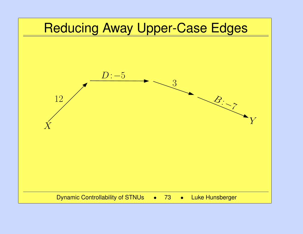
Reducing Away Upper-Case Edges
YX
12
3D :−5
B :−7
Dynamic Controllability of STNUs • 73 • Luke Hunsberger
73
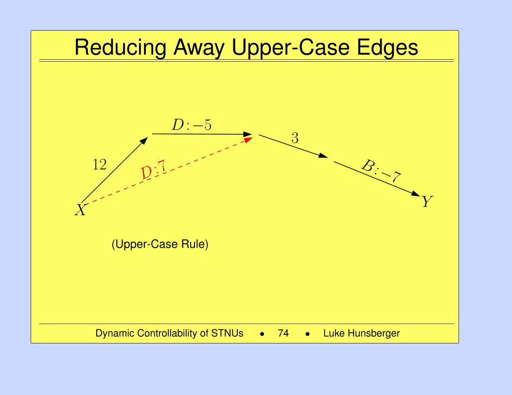
Reducing Away Upper-Case Edges
YX
12
3D :−5
B :−7D : 7
(Upper-Case Rule)
Dynamic Controllability of STNUs • 74 • Luke Hunsberger
74
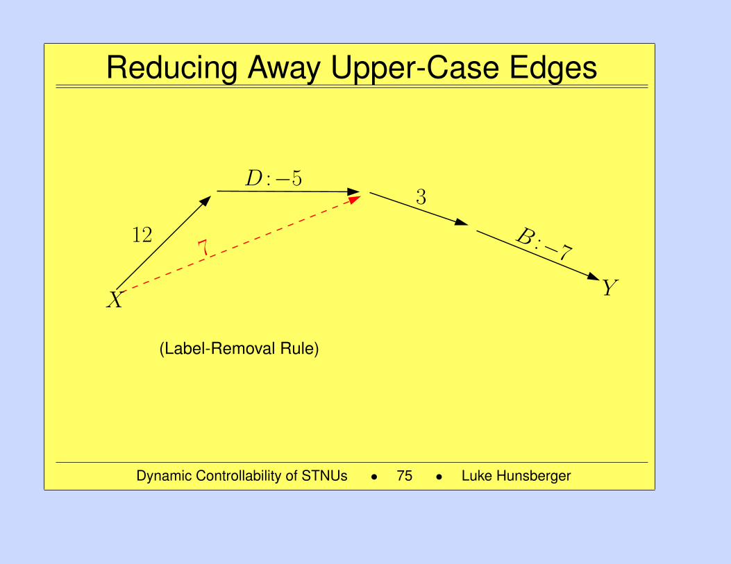
Reducing Away Upper-Case Edges
YX
12
3D :−5
B :−77
(Label-Removal Rule)
Dynamic Controllability of STNUs • 75 • Luke Hunsberger
75
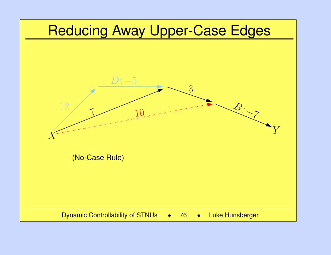
Reducing Away Upper-Case Edges
YX
12
3D :−5
B :−77 10
(No-Case Rule)
Dynamic Controllability of STNUs • 76 • Luke Hunsberger
76
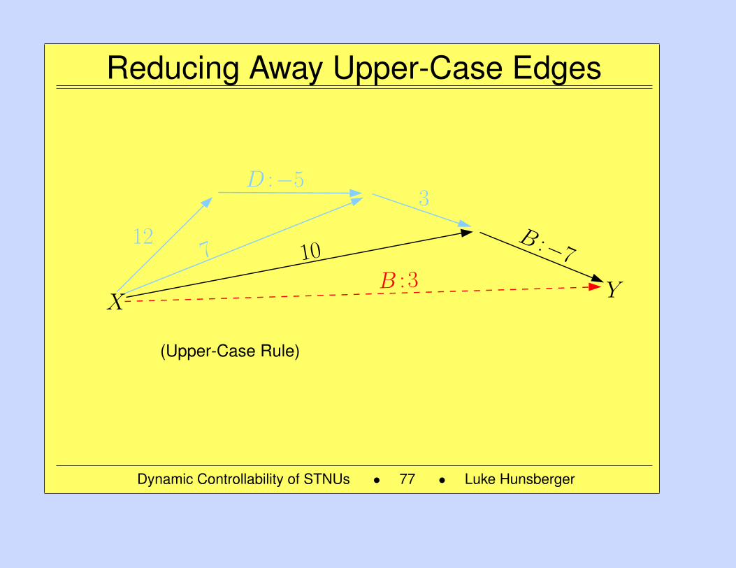
Reducing Away Upper-Case Edges
YX
12
3D :−5
B :−77 10
B : 3
(Upper-Case Rule)
Dynamic Controllability of STNUs • 77 • Luke Hunsberger
77
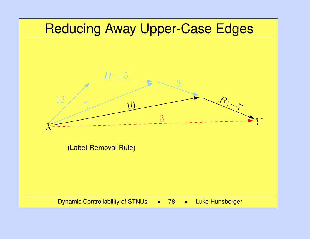
Reducing Away Upper-Case Edges
YX
12
3D :−5
B :−77 10
3
(Label-Removal Rule)
Dynamic Controllability of STNUs • 78 • Luke Hunsberger
78
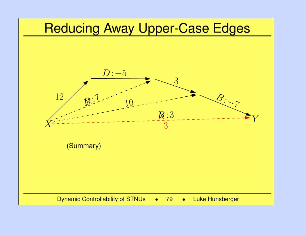
Reducing Away Upper-Case Edges
YX 3
D : 712
3D :−5
B :−710
B : 3
(Summary)
Dynamic Controllability of STNUs • 79 • Luke Hunsberger
79
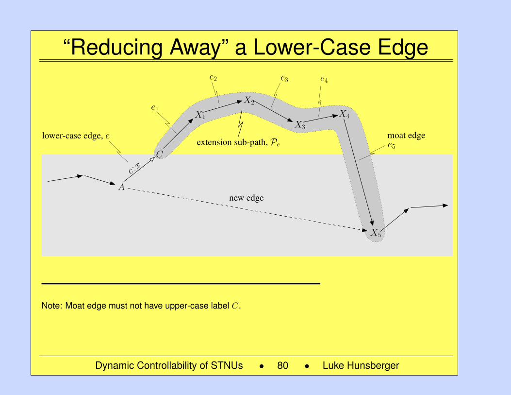
“Reducing Away” a Lower-Case Edge
moat edgee5
X4
X3
e4e3e2
X2
lower-case edge, e
C
e1X1
X5
A
c :x
extension sub-path, Pe
new edge
Note: Moat edge must not have upper-case label C.
Dynamic Controllability of STNUs • 80 • Luke Hunsberger
80
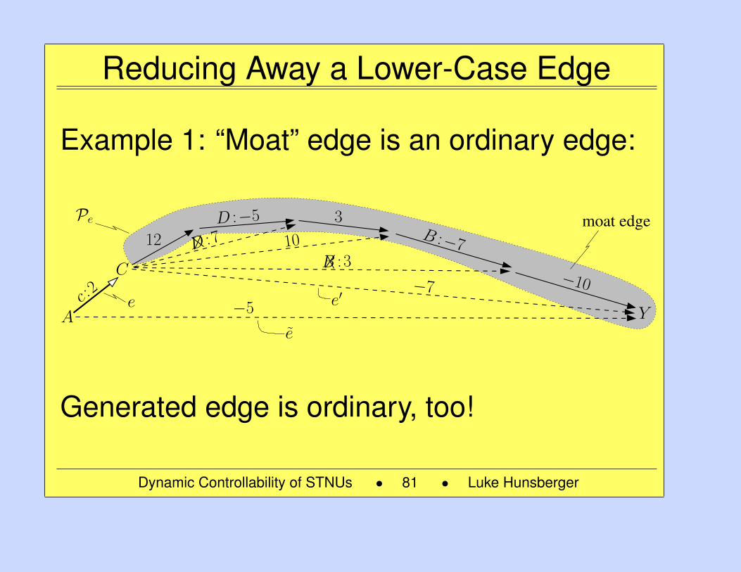
Reducing Away a Lower-Case Edge
Example 1: “Moat” edge is an ordinary edge:
C
e′
e
e
Pe
A
D : 712
D :−5 3B :−7
moat edge
Y
10
c :2 −7
−10
−5
B : 3
Generated edge is ordinary, too!
Dynamic Controllability of STNUs • 81 • Luke Hunsberger
81
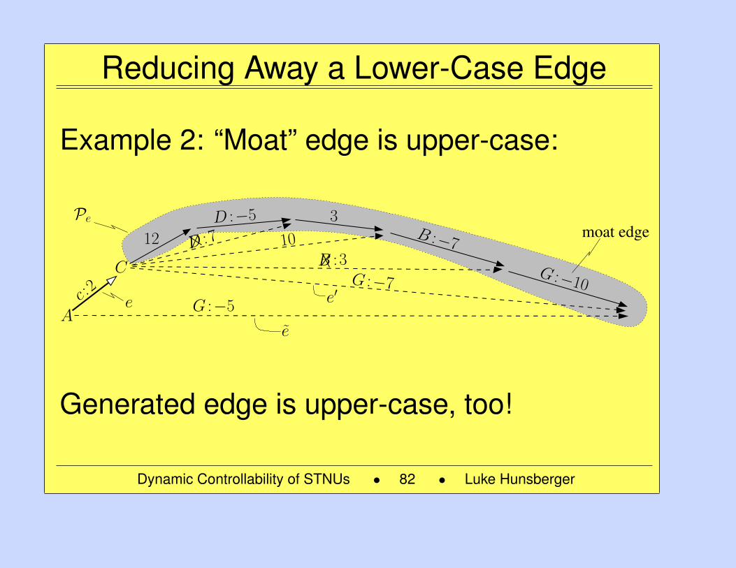
Reducing Away a Lower-Case Edge
Example 2: “Moat” edge is upper-case:
C
e′eA
e
PeD : 712
D :−5 3B :−7
moat edge10
G :−7
G :−5
G :−10c :
2
B : 3
Generated edge is upper-case, too!
Dynamic Controllability of STNUs • 82 • Luke Hunsberger
82
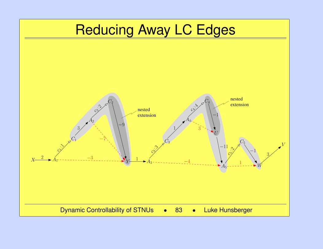
Reducing Away LC Edges
X A1
C1
3
C2
Y A3
C3
A4
C4
A5
C5
W
3
V−1
−1
U
−11
1
c 1: 1
2
−9
1
c 3: 3
c 4: 4
c 5: 2
c 2: 2
A2
−7
−3
3
−4 1
nestedextension
nestedextension
Dynamic Controllability of STNUs • 83 • Luke Hunsberger
83
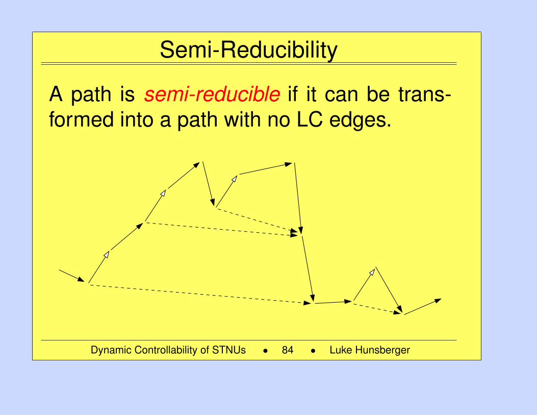
Semi-Reducibility
A path is semi-reducible if it can be trans-formed into a path with no LC edges.
Dynamic Controllability of STNUs • 84 • Luke Hunsberger
84
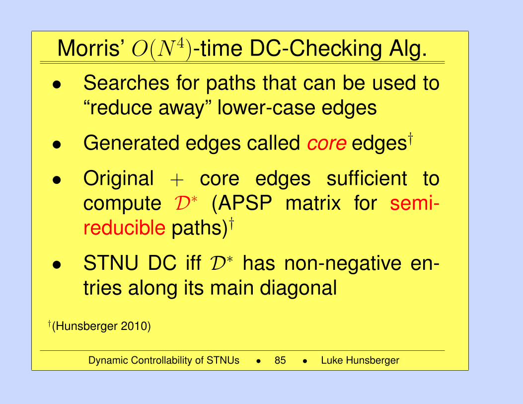
Morris’ O(N 4)-time DC-Checking Alg.• Searches for paths that can be used to
“reduce away” lower-case edges
• Generated edges called core edges†
• Original + core edges sufficient tocompute D∗ (APSP matrix for semi-reducible paths)†
• STNU DC iff D∗ has non-negative en-tries along its main diagonal
†(Hunsberger 2010)
Dynamic Controllability of STNUs • 85 • Luke Hunsberger
85
Executing STNUs
Dynamic Controllability of STNUs • 86 • Luke Hunsberger
86
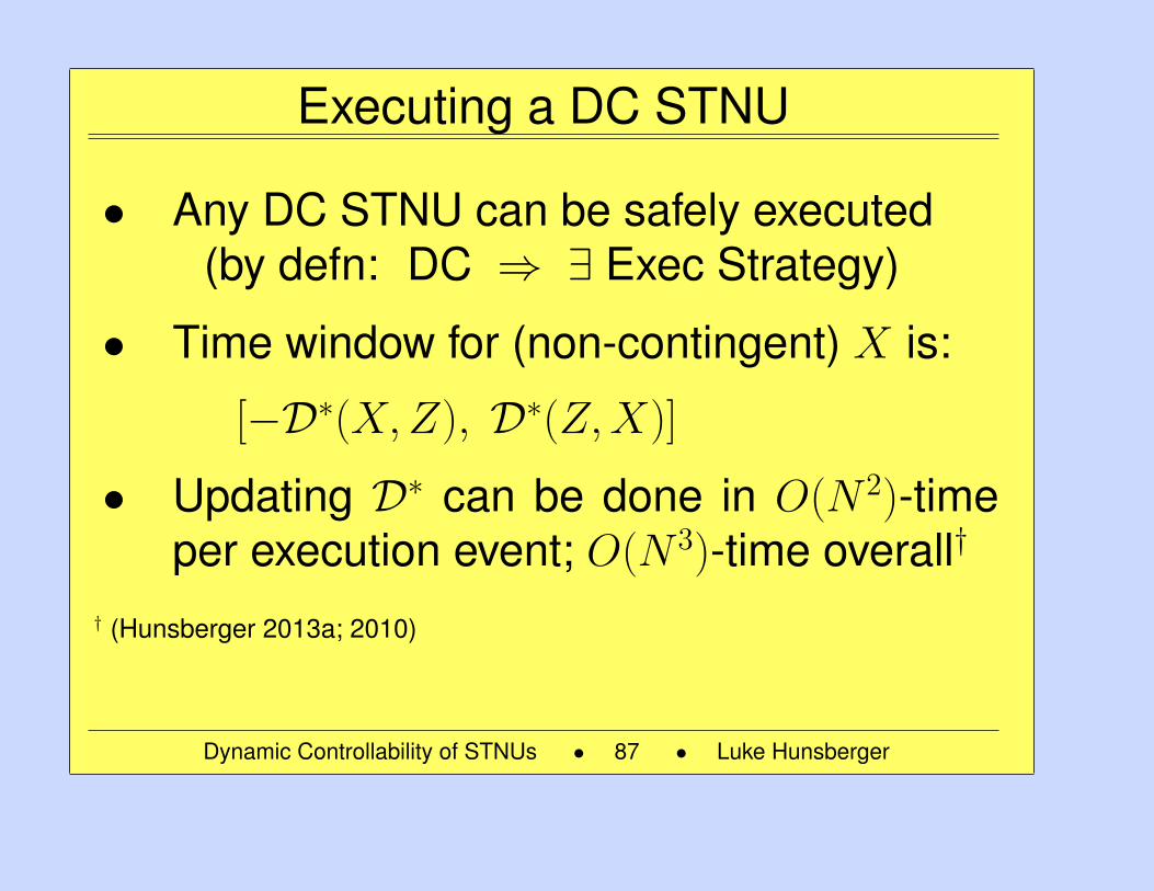
Executing a DC STNU
• Any DC STNU can be safely executed(by defn: DC ⇒ ∃ Exec Strategy)
• Time window for (non-contingent) X is:
[−D∗(X,Z), D∗(Z,X)]
• Updating D∗ can be done in O(N 2)-timeper execution event; O(N 3)-time overall†
† (Hunsberger 2013a; 2010)
Dynamic Controllability of STNUs • 87 • Luke Hunsberger
87
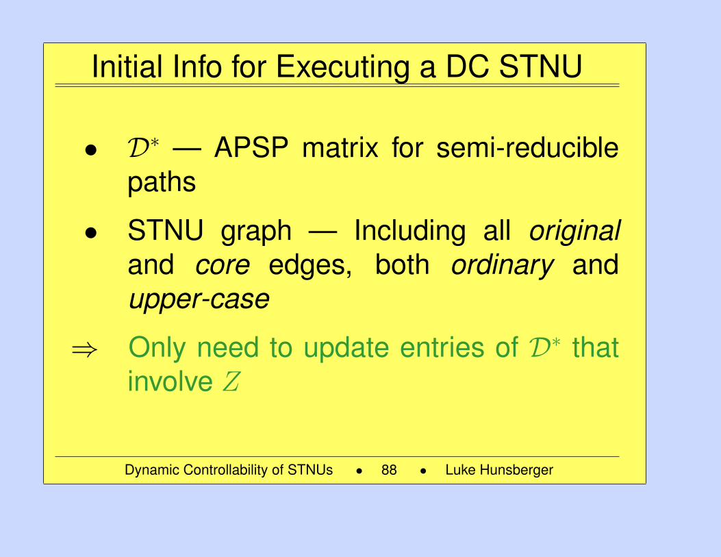
Initial Info for Executing a DC STNU
• D∗ — APSP matrix for semi-reduciblepaths
• STNU graph — Including all originaland core edges, both ordinary andupper-case
⇒ Only need to update entries of D∗ thatinvolve Z
Dynamic Controllability of STNUs • 88 • Luke Hunsberger
88
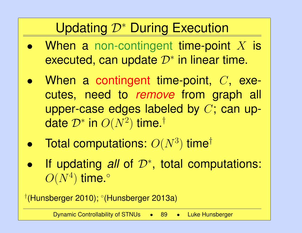
Updating D∗ During Execution• When a non-contingent time-point X is
executed, can update D∗ in linear time.
• When a contingent time-point, C, exe-cutes, need to remove from graph allupper-case edges labeled by C; can up-date D∗ in O(N 2) time.†
• Total computations: O(N 3) time†
• If updating all of D∗, total computations:O(N 4) time.
†(Hunsberger 2010); (Hunsberger 2013a)
Dynamic Controllability of STNUs • 89 • Luke Hunsberger
89
Magic Loops in STNUs
Dynamic Controllability of STNUs • 90 • Luke Hunsberger
90
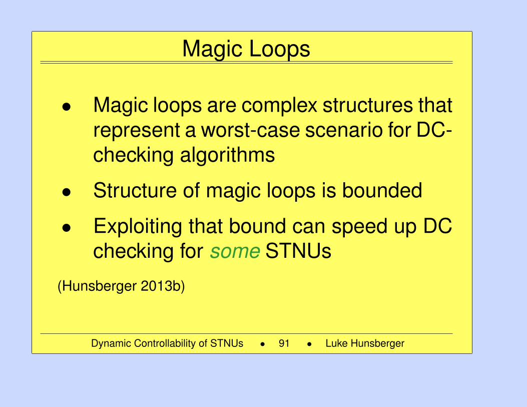
Magic Loops
• Magic loops are complex structures thatrepresent a worst-case scenario for DC-checking algorithms
• Structure of magic loops is bounded
• Exploiting that bound can speed up DCchecking for some STNUs
(Hunsberger 2013b)
Dynamic Controllability of STNUs • 91 • Luke Hunsberger
91
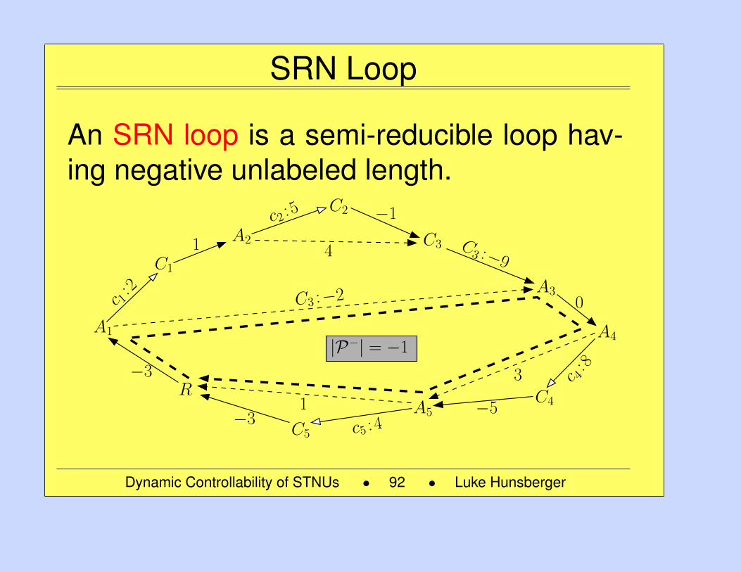
SRN Loop
An SRN loop is a semi-reducible loop hav-ing negative unlabeled length.
0
A4|P−| = −1
C2
c 1: 2
1
−1
−3
C1
A24
A1
c2 : 5
R
C3
c5 : 4A5
C5
A3
C4−5
c 4: 8
C3 :−9
C3 :−2
−3
1
3
Dynamic Controllability of STNUs • 92 • Luke Hunsberger
92
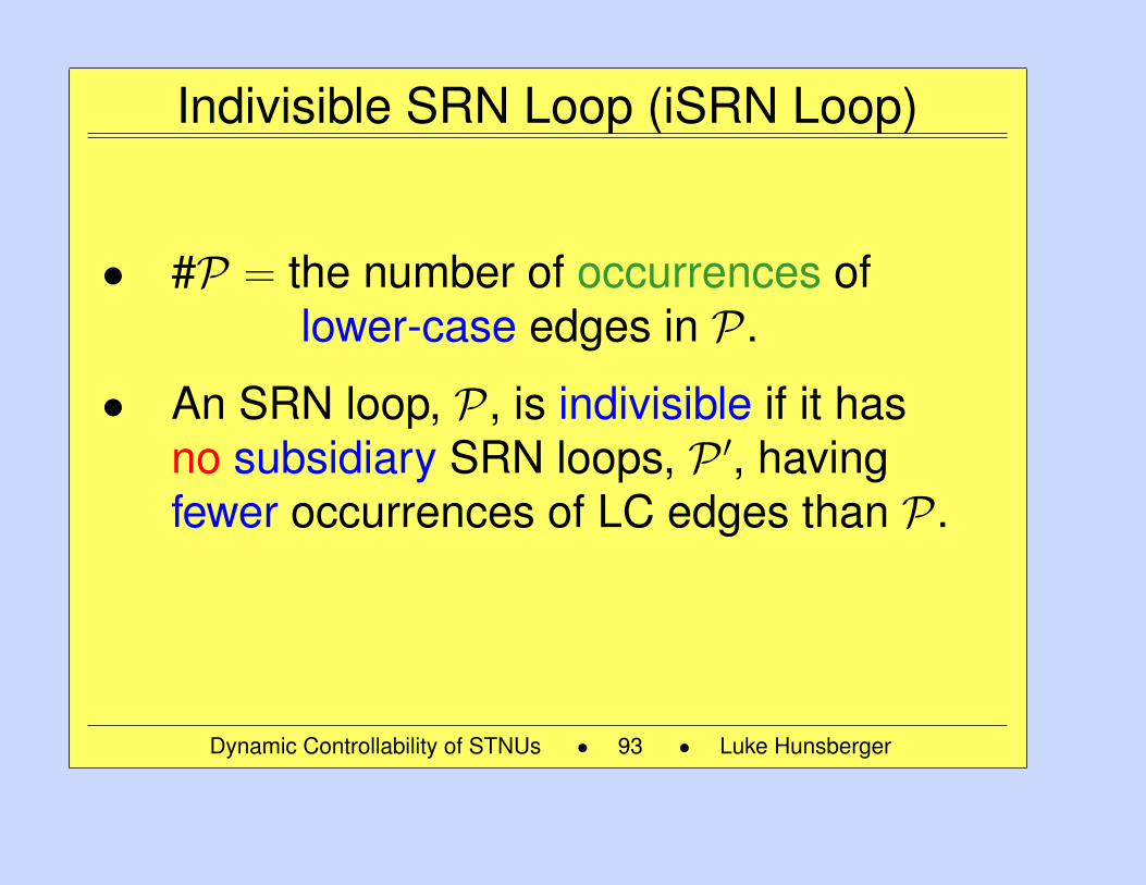
Indivisible SRN Loop (iSRN Loop)
• #P = the number of occurrences oflower-case edges in P.
• An SRN loop, P, is indivisible if it hasno subsidiary SRN loops, P ′, havingfewer occurrences of LC edges than P.
Dynamic Controllability of STNUs • 93 • Luke Hunsberger
93
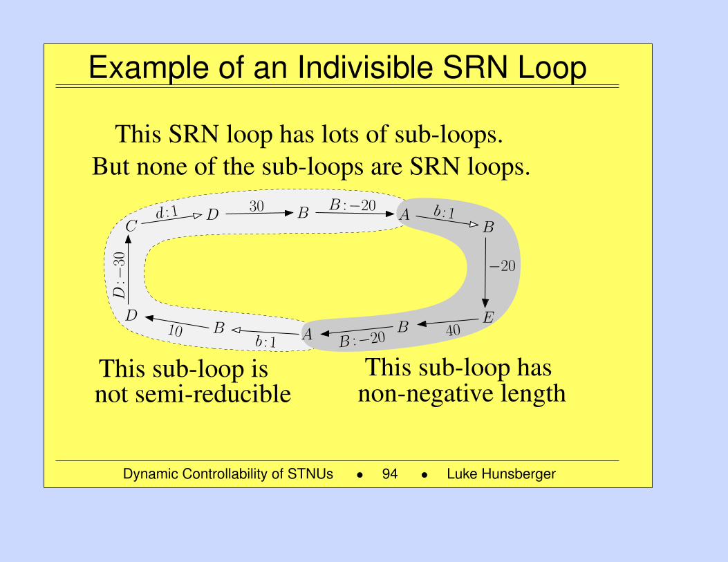
Example of an Indivisible SRN Loop
B
E
C
D
−20
BD A
BAB
B :−20 b : 1
B :−2010
D:−
30
b : 1
30d : 1
40
non-negative lengthThis sub-loop hasThis sub-loop is
not semi-reducible
But none of the sub-loops are SRN loops.This SRN loop has lots of sub-loops.
Dynamic Controllability of STNUs • 94 • Luke Hunsberger
94
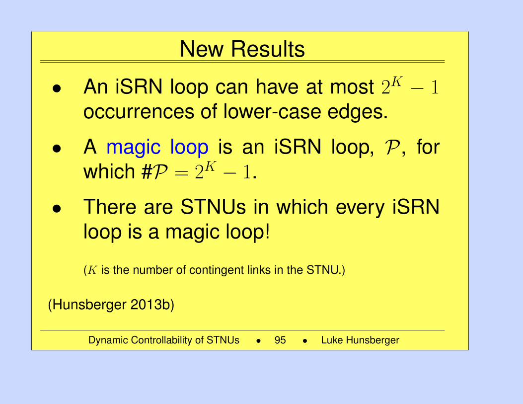
New Results
• An iSRN loop can have at most 2K − 1occurrences of lower-case edges.
• A magic loop is an iSRN loop, P, forwhich #P = 2K − 1.
• There are STNUs in which every iSRNloop is a magic loop!
(K is the number of contingent links in the STNU.)
(Hunsberger 2013b)
Dynamic Controllability of STNUs • 95 • Luke Hunsberger
95
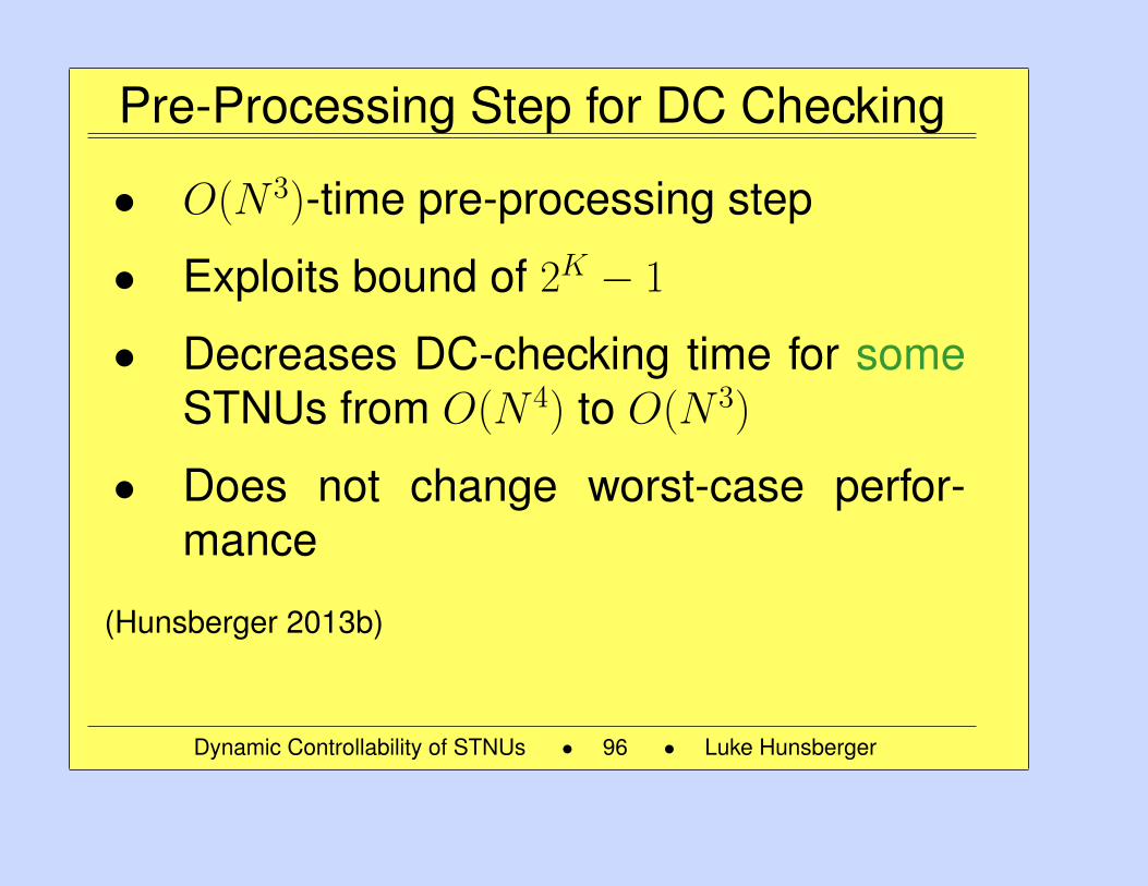
Pre-Processing Step for DC Checking
• O(N 3)-time pre-processing step
• Exploits bound of 2K − 1
• Decreases DC-checking time for someSTNUs from O(N 4) to O(N 3)
• Does not change worst-case perfor-mance
(Hunsberger 2013b)
Dynamic Controllability of STNUs • 96 • Luke Hunsberger
96
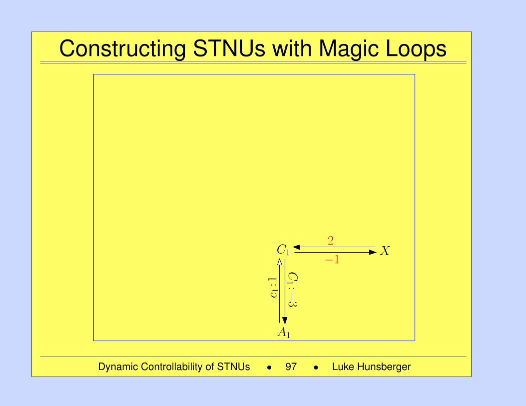
Constructing STNUs with Magic Loops
C1
C1 :−
3
A1
X−1
2
c 1:1
Dynamic Controllability of STNUs • 97 • Luke Hunsberger
97
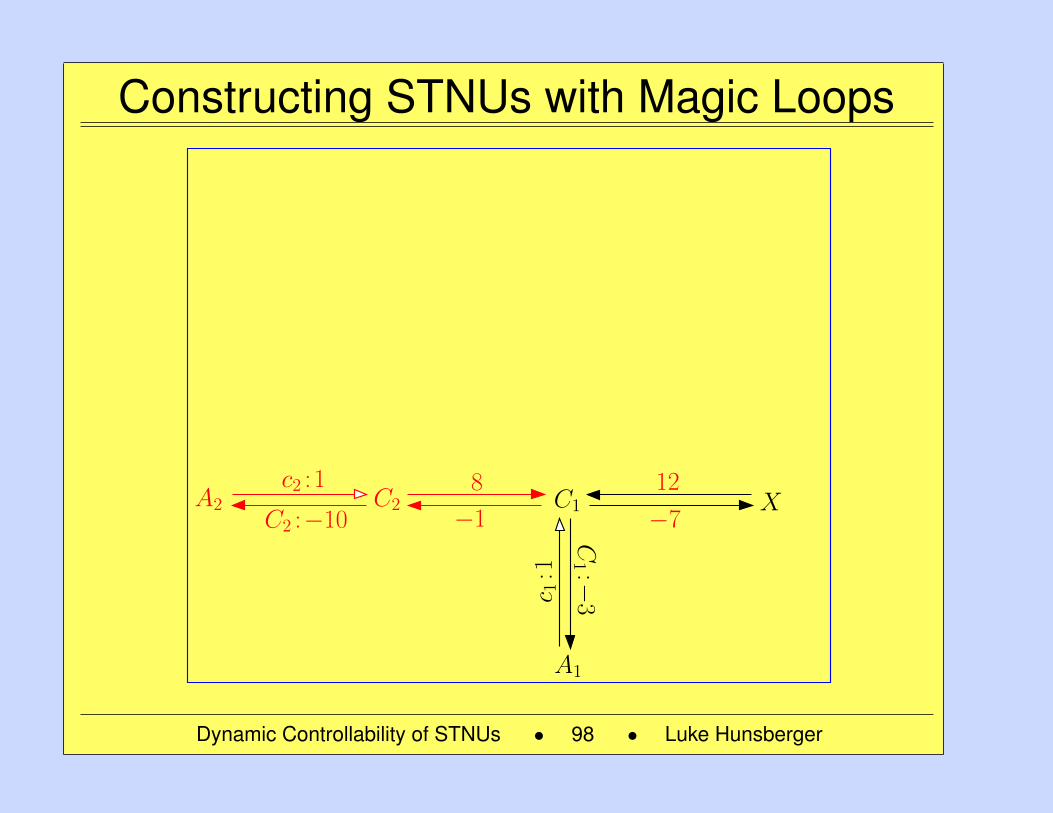
Constructing STNUs with Magic Loops
C1
C1 :−
3
A1
X12
−7c 1
:1
A2
c2 : 1 8C2 −1C2 :−10
Dynamic Controllability of STNUs • 98 • Luke Hunsberger
98
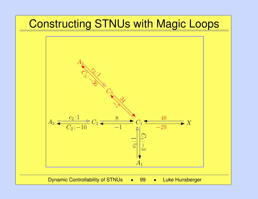
Constructing STNUs with Magic Loops
C1
C1 :−
3
C2 :−10 −1
8
A1
c2 : 1C2 XA2
C3
A3c3 : 1
48
−29
C3 :−
36
c 1:1
34−7
Dynamic Controllability of STNUs • 99 • Luke Hunsberger
99
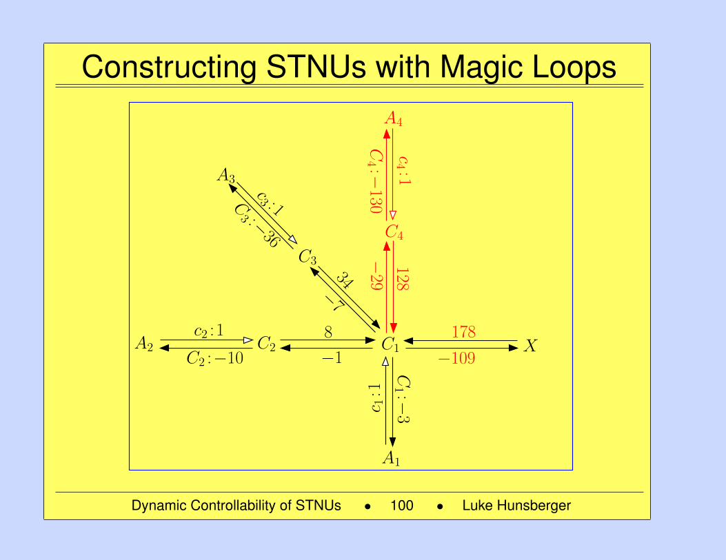
Constructing STNUs with Magic Loops
C1
C1 :−
3
C2 :−10 −1
8
A1
c2 : 1C2 XA2
C3
A3
C3 :−
36
c3 : 1
C4
A4
178
−109c 1
:1
c4 :1
128
C4 :−
130−
2934
−7
Dynamic Controllability of STNUs • 100 • Luke Hunsberger
100
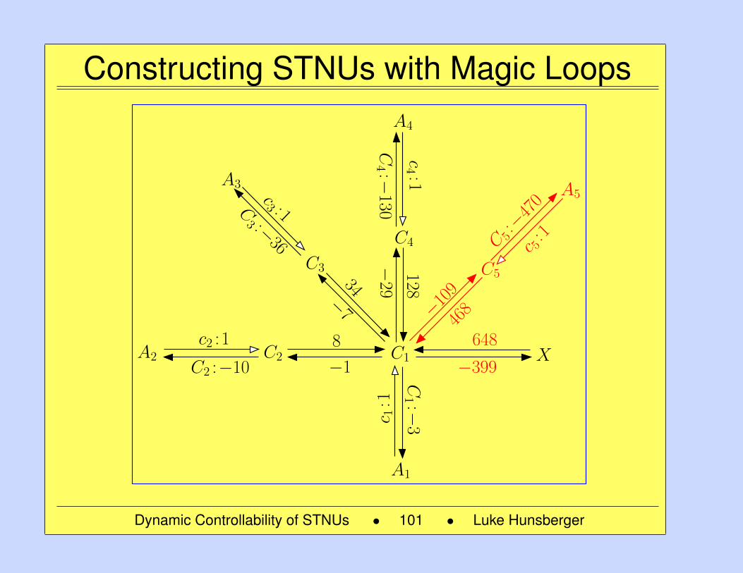
Constructing STNUs with Magic Loops
C1
C1 :−
3
C2 :−10 −1
8
A1
c2 : 1C2 XA2
C3
A3
C3 :−
36
c3 : 1
C4
A4
A5
C 5:−
470
c 1:1
−399
648c4 :1
128
C5
−109
c 5: 1
468
C4 :−
130−
2934
−7
Dynamic Controllability of STNUs • 101 • Luke Hunsberger
101
Conclusions
Dynamic Controllability of STNUs • 102 • Luke Hunsberger
102
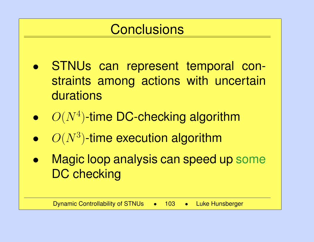
Conclusions
• STNUs can represent temporal con-straints among actions with uncertaindurations
• O(N 4)-time DC-checking algorithm
• O(N 3)-time execution algorithm
• Magic loop analysis can speed up someDC checking
Dynamic Controllability of STNUs • 103 • Luke Hunsberger
103
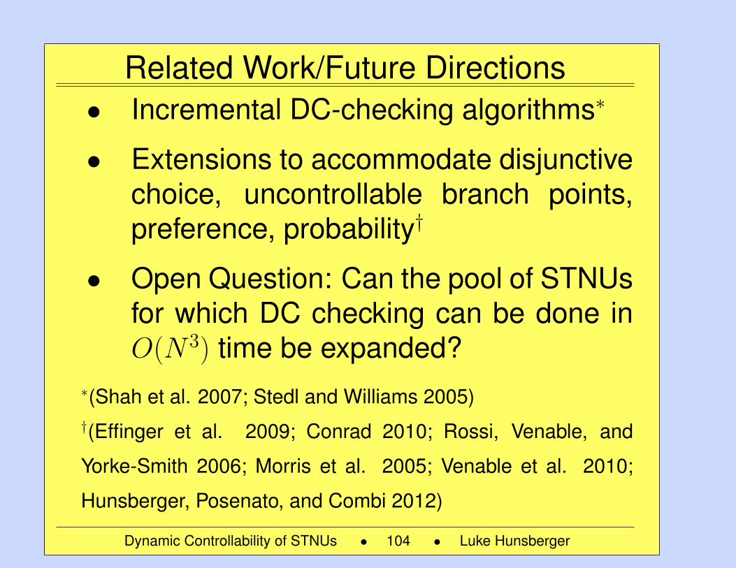
Related Work/Future Directions• Incremental DC-checking algorithms∗
• Extensions to accommodate disjunctivechoice, uncontrollable branch points,preference, probability†
• Open Question: Can the pool of STNUsfor which DC checking can be done inO(N 3) time be expanded?
∗(Shah et al. 2007; Stedl and Williams 2005)†(Effinger et al. 2009; Conrad 2010; Rossi, Venable, and
Yorke-Smith 2006; Morris et al. 2005; Venable et al. 2010;
Hunsberger, Posenato, and Combi 2012)
Dynamic Controllability of STNUs • 104 • Luke Hunsberger
104
STNU-related talk at ICAPS-2013
Incremental Dynamic Controllability Revisited
—Mikael Nilsson, Jonas Kvarnstrm,and Patrick Doherty
—on Friday!
Dynamic Controllability of STNUs • 105 • Luke Hunsberger
105
References
• Cesta, A., and Oddi, A. 1996. Gaining efficiency and flexibility in the simple temporal problem. In Proceedings of the Third InternationalWorkshop on Temporal Representation and Reasoning (TIME-96), 45–50. IEEE.
• Conrad, P. R. 2010. Flexible execution of plans with choice and uncertainty. Master’s thesis, Massachusetts Institute of Technology.
• Cormen, T. H.; Leiserson, C. E.; and Rivest, R. L. 1990. Introduction to Algorithms. Cambridge, MA: The MIT Press.
• Dechter, R.; Meiri, I.; and Pearl, J. 1991. Temporal constraint networks. Artificial Intelligence 49:61–95.
• Demetrescu, C., and Italiano, G. 2002. A new approach to dynamic all pairs shortest paths. Technical Report ALCOMFT-TR-02-92,ALCOM-FT. To appear in Proceedings of the 35th Annual ACM Symposium on Theory of Computing (STOC’03), San Diego, California,June 2003.
• Effinger, R.; Williams, B.; Kelly, G.; and Sheehy, M. 2009. Dynamic controllability of temporally-flexible reactive programs. In Gerevini,A.; Howe, A.; Cesta, A.; and Refanidis, I., eds., Proceedings of the Nineteenth International Conference on Automated Planning andScheduling (ICAPS 09). AAAI Press.
• Even, S., and Gazit, H. 1985. Updating distances in dynamic graphs. Methods of Operations Research 49:371–387.
• Gerevini, A.; Perini, A.; and Ricci, F. 1996. Incremental algorithms for managing temporal constraints. Technical Report IRST-9605-07,IRST.
• Hunsberger, L.; Posenato, R.; and Combi, C. 2012. The dynamic controllability of conditional STNs with uncertainty. In Proceedingsof the Planning and Plan Execution for Real-World Systems: Principles and Practices (PlanEx) Workshop associated with the ICAPS-2012Conference, 121–128.
• Hunsberger, L. 2008. A practical temporal constraint management system for real-time applications. In Proceedings of the EuropeanConference on Artificial Intelligence (ECAI-2008), 553–557. IOS Press.
• Hunsberger, L. 2009. Fixing the semantics for dynamic controllability and providing a more practical characterization of dynamic executionstrategies. In Proceedings of the 16th International Symposium on Temporal Representation and Reasoning (TIME-2009), 155–162. IEEEComputer Society.
• Hunsberger, L. 2010. A fast incremental algorithm for managing the execution of dynamically controllable temporal networks. In Proceed-ings of the 17th International Symposium on Temporal Representation and Reasoning (TIME-2010), 121–128. IEEE.
• Hunsberger, L. 2013a. A faster execution algorithm for dynamically controllable stnus. In Proceedings of the 20th International Symposiumon Temporal Representation and Reasoning (TIME-13), To Appear.
• Hunsberger, L. 2013b. Magic loops in simple temporal networks with uncertainty. In Proceedings of the Fifth International Conference onAgents and Artificial Intelligence (ICAART-2013).
• Morris, P. H., and Muscettola, N. 2005. Temporal dynamic controllability revisited. In The Twentieth National Conference on ArtificialIntelligence (AAAI-2005), 1193–1198. The MIT Press.
• Morris, R.; Morris, P.; Khatib, L.; and Yorke-Smith, N. 2005. Temporal constraint reasoning with preferences and probabilities. In Brafman,R., and Junker, U., eds., Proceedings of the IJCAI-05 Multidisciplinary Workshop on Advances in Preference Handling, 150–155.
106
• Morris, P.; Muscettola, N.; and Vidal, T. 2001. Dynamic control of plans with temporal uncertainty. In Seventeenth International JointConference on Artificial Intelligence (IJCAI-01), 494–499. Morgan Kaufmann.
• Morris, P. 2006. A structural characterization of temporal dynamic controllability. In Principles and Practice of Constraint Programming(CP 2006), volume 4204 of Lecture Notes in Computer Science. Springer. 375–389.
• Muscettola, N.; Morris, P.; and Tsamardinos, I. 1998. Reformulating temporal plans for efficient execution. In Proceedings of the SixthInternational Conference on Principles of Knowledge Representation and Reasoning (KR-98).
• Ramalingam, G., and Reps, T. 1996. On the computational complexity of dynamic graph problems. Theoretical Computer Science158:233–277.
• Rohnert, H. 1985. A dynamization of the all pairs least cost path problem. In Mehlhorn, K., ed., 2nd Symposium of Theoretical Aspects ofComputer Science (STACS 85), volume 182 of Lecture Notes in Computer Science. Springer. 279–286.
• Rossi, F.; Venable, K. B.; and Yorke-Smith, N. 2006. Uncertainty in soft temporal constraint problems: A general framework and control-lability algorithms for the fuzzy case. Journal of Artificial Intelligence Research 27:617–674.
• Shah, J.; Stedl, J.; Robertson, P.; and Williams, B. C. 2007. A fast incremental algorithm for maintaining dispatchability of partiallycontrollable plans. In Mark Boddy et al., ed., Proceedings of the Seventeenth International Conference on Automated Planning and Scheduling(ICAPS 2007). AAAI Press.
• Stedl, J., and Williams, B. C. 2005. A fast incremental dynamic controllability algorithm. In Proceedings of the ICAPS Workshop on PlanExecution: A Reality Check, 69–75.
• Tsamardinos, I.; Muscettola, N.; and Morris, P. 1998. Fast transformation of temporal plans for efficient execution. In Proceedings of theFifteenth National Conference on Artificial Intelligence (AAAI-98). Cambridge, MA: The MIT Press. 254–261.
• Venable, K. B.; Volpato, M.; Peintner, B.; and Yorke-Smith, N. 2010. Weak and dynamic controllability of temporal problems withdisjunctions and uncertainty. In Proceedings of COPLAS 2010: ICAPS Workshop on Constraint Satisfaction Techniques for Planning andScheduling Problems, 50–59.
107


