
The Impact of Group Purchasing Organizations on1
Healthcare-Product Supply Chains2
Qiaohai (Joice) Hu1, Leroy B. Schwarz1, and Nelson A. Uhan23
1Krannert School of Management, Purdue University, West Lafayette, IN, USA.4
{hu23, lschwarz}@purdue.edu5
2School of Industrial Engineering, Purdue University, West Lafayette, IN, USA. [email protected]
May 20117
Abstract. This paper examines the impact of group purchasing organizations (GPOs) on healthcare-8
product supply chains. The supply chain we examine consists of a profit-maximizing manufacturer with a9
quantity-discount schedule that is nonincreasing in quantity and ensures nondecreasing revenue, a profit-10
maximizing GPO, a competitive source selling at a fixed unit price, and n providers (e.g., hospitals) with11
fixed demands for a single product. Each provider seeks to minimize its total purchasing cost (i.e., the cost of12
the goods plus the provider’s own fixed transaction cost). Buying through the GPO offers providers possible13
cost reductions, but may involve a membership fee. Selling through the GPO offers the manufacturer possibly14
higher volumes, but requires that the manufacturer pay the GPO a contract administration fee (CAF); i.e., a15
percentage of all revenue contracted through it. Using a game-theoretic model, we examine questions about16
this supply chain, including how the presence of a GPO affects the providers’ total purchasing costs. We also17
address the controversy about whether Congress should amend the Social Security Act, which, under current18
law, permits CAFs. Among other things, we conclude that although CAFs affect the distribution of profits19
between manufacturers and GPOs, they do not affect the providers’ total purchasing costs.20
1 Introduction21
Group purchasing organizations (GPOs) play a very important role in the supply chains for healthcare22
products. A survey by Burns and Lee (2008) reports that nearly 85% of U.S. hospitals route 50%23
or more of their commodity-item spending, and 80% route 50% or more of their pharmaceutical24
spending through GPOs. According to the Health Industry Group Purchasing Association (HIGPA),25
Copyright 2011 by the authors. All rights reserved. This work may not be reproduced or distributed in any form orby any means—graphic, electronic, or mechanical, including photocopying, recording, or information storage—withoutthe express written consent of the authors.
The research upon which this manuscript is based was funded entirely by Purdue University.
1

“nearly every hospital in the U.S. (approximately 96% to 98%) chooses to utilize GPO contracts for26
their purchasing functions.”27
U.S. healthcare-product GPOs started in the late 1800s, and grew rapidly in the late 1970s and28
early 1980s, partly in response to competition from for-profit hospitals, and partly in response to29
pressure to reduce costs from third-party payers. GPOs evolved to become significant “players” in30
healthcare-product supply chains following a 1987 amendment to the Social Security Act, which31
permits GPOs to charge contract administration fees (CAFs) to manufacturers. CAFs are essentially32
commissions paid by manufacturers to GPOs on sales to the GPO’s members. Prior to the 198733
amendment, CAFs had been prohibited.34
CAFs are controversial. They are criticized by manufacturers, who complain that they are forced35
to charge higher prices for all products, whether they are sold through a GPO or not, in order to36
recover the CAFs paid to GPOs. Sethi (2006) estimates that “... GPOs generate excess revenue37
in the range of $5-6B, which legitimately belongs to its members ...” Singer (2006), in reference38
to the so-called “safe harbor” provisions of the 1987 amendment, says “the elimination of the safe39
harbor (provisions) ... would generate large savings for the federal government.” Others assert that40
CAFs create a conflict of interest, i.e., that GPOs do not have an incentive to negotiate the lowest41
possible prices for their members because the CAF is based on that negotiated price.42
The fundamental rationale for joining a GPO is that a provider will incur a lower total purchasing43
cost—that is, the cost of the given product plus the provider’s own fixed transaction cost, or fixed44
contracting cost—by buying through the GPO than by contracting for that same item directly with45
a manufacturer. GPOs assert that they are able to lower their provider-members price per unit46
by employing market intelligence and product expertise that no single member could afford, and47
by contracting for the group’s combined purchase quantity. GPOs are able to lower a provider’s48
fixed contracting cost by spreading its own, presumably higher, fixed contracting cost over its49
many members. Schneller and Smeltzer (2006, p. 218, Table 1.3) identify several components of a50
provider’s fixed contracting cost, among them determining product use and requirements, preparing51
bids or requests for proposal, and conducting product evaluation.52
Schneller and Smeltzer (2006) report that a provider’s fixed contracting cost is $3,116 per53
contract if a provider contracts directly with a manufacturer, and $1,749 per contract if a provider54
contracts through a GPO: a difference of $1,367 in fixed contracting cost per contract. We refer55
2

to this difference as the GPO’s contracting efficiency ; i.e., the reduction of the provider’s fixed56
contracting cost if it contracts through a GPO instead of contracting directly with a manufacturer.57
It should be noted that Schneller and Schmeltzer’s estimate of GPO contracting efficiency ($1,367)58
is based on case studies conducted by Novation, a GPO, and cannot be independently confirmed.59
Nonetheless, no one in the industry questions the contracting efficiency of GPOs, not even GPO60
critics, such as Sethi (2006) and Singer (2006) cited above.61
GPOs earn revenue from several sources: membership fees charged to provider-members, CAFs62
charged to manufacturers, administrative fees charged to distributors authorized to distribute63
products under the GPOs’ contracts, and miscellaneous service fees. According to Burns and Lee64
(2008), GPO membership fees are “nonnegligible” for providers; e.g., $300,000 – $600,000 for a small65
hospital system anchored around a teaching hospital. However, CAFs are the primary source of66
GPO revenues (Burns 2002, p. 69).67
In this paper, we assume that healthcare providers have four important characteristics, which68
we believe represent practice. First, each provider seeks to minimize its total purchasing cost (i.e.,69
the cost of the goods purchased plus the provider’s own fixed transaction cost), not merely the cost70
of the goods themselves. Second, we assume that each provider’s demand, denoted as its purchasing71
requirement, is fixed. Third, providers who belong to GPOs are not required to purchase specific72
products through the GPO. Hence, providers are free to negotiate directly with manufacturers or73
other suppliers. Fourth, providers are highly diverse, particularly with respect to size, and hence,74
the size of their purchasing requirements. Regardless of these differences in size, there is evidently75
enough homogeneity in other respects to provide common ground for both small and large providers76
to belong to healthcare GPOs (Arnold 1997). Of course, our results apply to the extent that77
these assumptions hold. See §8 for comments on the impact of our paper’s major assumptions and78
limitations on our results.79
Given the significant, controversial role that GPOs play in healthcare-product supply chains,80
our research asks the following questions: (1) Do providers experience lower prices or lower total81
purchasing costs with a GPO in the supply chain? (2) Do CAFs mean higher prices paid by82
providers? (3) How does the presence of the GPO affect manufacturer profits? (4) What affects83
GPO profits? (5) How are supply-chain profits divided between the manufacturer and the GPO,84
and how is the division influenced by the “power” of the GPO? The answers to these questions have85
3

implications for government policy and, in practical terms, for the cost of healthcare.86
In order to explore these issues, we analyze a game-theoretic model that includes a profit-87
maximizing GPO, a profit-maximizing manufacturer whom the GPO has already chosen to contract88
with, and n providers with various purchasing requirements. We also assume the presence of a89
competitive source that sells the product at a fixed exogenous price. The salient features of our90
model, which in combination are characteristics of healthcare GPOs, are: (1) the GPO’s contracting91
efficiency; (2) CAFs that GPOs charge to manufacturers for GPO-contracted sales; and (3) GPO92
membership fees.93
The sequence of events in our model is as follows. First, the manufacturer and the GPO negotiate94
the size of the CAF that the manufacturer will pay the GPO for on-contract purchases. We do not95
model this negotiation directly. Instead, the CAF is a parameter whose value represents the “power”96
of the manufacturer versus the GPO; e.g., the higher the CAF, the more powerful the GPO. Note97
that the “safe harbor” provisions of the 1987 amendment nominally limit CAFs to 3%; however,98
exceptions are permitted. Second, given the CAF, the providers’ purchasing requirements, and the99
price from the competitive source, the manufacturer determines a quantity-discount schedule.100
Third, the GPO determines what on-contract price to offer providers in order to maximize its101
profit. The GPO collects a CAF from the manufacturer for on-contract sales, and may charge a102
fixed membership fee to the providers who decide to buy through it. In order to represent the103
GPO as a profit maximizer, we have modeled it as buying from the manufacturer at one price and104
selling to its members at another price. In fact, GPOs neither buy nor sell products. Instead, they105
negotiate the on-contract prices that their members pay for a manufacturer’s products. Hence, if106
the manufacturer agrees, the member’s on-contract price can be set higher than the manufacturer’s107
own price for that quantity, thereby generating a positive margin for the GPO.108
Finally, each provider splits its requirement among the GPO, the manufacturer, and the109
competitive source, in order to minimize its total purchasing cost. We assume that the providers110
incur the same fixed contracting cost when buying from the manufacturer or from the competitive111
source but a lower fixed contracting cost when buying through the GPO because of the GPO’s112
contracting efficiency.113
Before continuing, a few comments about our model. First, modeling a supply chain with a114
single GPO is reasonable. Although Burns and Lee (2008) report that 41% of the providers surveyed115
4
belong to more than one GPO, they “... route most of their purchases through a single national116
alliance ... and utilize (another) only for specific contracts in limited supply areas.” Second, GPO117
contracts are typically “rebid” every 3 to 5 years, depending on the GPO and the type of product.118
We do not model this bidding process. Instead, our model assumes that bidding has already taken119
place for a given item and that a single manufacturer has been chosen by the GPO to sell products120
to its members. We do not model what the GPO does with its profits. It should be noted that121
some GPOs are member-owned or partially member-owned. In such cases, the provider-members122
receive a share of the GPO’s profits. We also do not account for the possibility that large providers123
may negotiate a portion of the GPOs’ CAF. We will return to these last two points in §8. We also124
do not examine the question of GPO formation since, as already noted, virtually every provider125
already belongs to a GPO. Hence, the important questions do not involve GPO formation but the126
impact of a GPO on the providers’ costs and the circumstances under which providers will avail127
themselves of GPO procurement services.128
The remainder of our paper is organized as follows. First, we define the game in its most129
general form: with a manufacturer that offers a quantity-discount schedule that is nonincreasing130
in quantity and ensures nondecreasing revenue, and with n providers with heterogeneous fixed131
purchasing requirements. For simplicity, we have assumed that the manufacturer’s production cost132
is zero. However, our results continue to hold, provided that the manufacturer’s marginal profit is133
marginally decreasing in quantity, and the manufacturer’s total profit is increasing in quantity (See134
§3). An analysis of the subgame-perfect Nash equilibrium strategies, specifically Lemmas 4.1 and135
4.2, provides a key structural result. This result provides the basis of an algorithm for computing136
an equilibrium solution for any parameterization of the general case.137
Following this analysis of the general case, we fully characterize the equilibrium of two special138
cases: the case of two heterogeneous providers, and the case of n identical providers, when the139
manufacturer’s quantity-discount schedule is linear. The analysis of these special cases provides140
unambiguous answers to the questions posed above. Then, using the algorithm in §4, we compute141
equilibria using similar parameterizations, but in more general cases; specifically, n heterogeneous142
providers with a linear discount schedule, 2 heterogeneous providers with a nonlinear discount143
schedule, and n identical providers with a nonlinear discount schedule. We observe that the144
characteristics of these equilibria are similar to the cases for which we have analytical solutions.145
5

Based on these observations, we believe these results on equilibria can be generalized (see §7).146
2 Literature review147
Healthcare GPOs have been discussed in the healthcare-management literature for years. Burns148
(2002) and Schneller and Smeltzer (2006) provide qualitative analyses of healthcare-GPO structure149
and function. More recently, Burns and Lee (2008), through a large-scale survey of hospital material150
managers, examined GPOs from the viewpoint of their members. They report: (1) 94% of survey151
respondents belong to a GPO, and (2) GPOs succeed in reducing health care costs by lowering152
product prices, particularly for commodity and pharmaceutical items.153
Two U.S. Government Accountability Office (GAO) reports (2003, 2010) provide background154
information about GPO business practices and the “safe harbor” provision in the Social Security155
Law. The 2003 report describes processes that GPOs use to select manufacturers’ products, the156
CAFs that they charge to manufacturers, their use of contracting strategies to obtain favorable157
prices, etc. The 2010 report describes the types of services that GPOs provide to members, how158
they fund these services, etc. An earlier GAO pilot survey from 2002, one often cited by GPO159
critics, reported that “a hospital’s use of a GPO contract did not guarantee that the hospital saved160
money: GPO’s prices were not always lower and were often higher than prices paid by hospitals161
negotiating with vendors directly.” This is one of the controversies that our analysis addresses.162
Our model, along with Hu and Schwarz (2011), provides the first theoretical analyses of healthcare163
GPOs. Hu and Schwarz (2011) examine some of the controversies about GPOs through the Hotelling164
model: a continuum of identical providers and two manufacturers. The providers decide whether165
to form a GPO when negotiating a price with the manufacturers. They show that forming a166
GPO increases competition between manufacturers, thus lowering prices for healthcare providers.167
They also demonstrate that the existence of lower off-contract prices is not, per se, evidence of168
anticompetitive behavior on the part of GPOs. Indeed, under certain circumstances, the presence169
of a GPO lowers off-contract prices. They also examine the consequences of eliminating the “safe170
harbor” provisions and conclude that it would not affect any party’s profits or costs.171
Due to limitations of the Hotelling model used in Hu and Schwarz (2011), hospitals are treated172
as identical, each having the same purchasing requirement. In contrast, our model has a discrete173
number of providers who may have different requirements, thus allowing us to examine the impact174
6

of the differences in healthcare providers’ purchasing requirements. In contrast to Hu and Schwarz175
(2011) where the GPO is formed by the providers, here the GPO is an independent entity that176
negotiates contracts for the providers by charging membership fees and CAFs, thereby possibly177
making a profit. Hence, to the best of our knowledge, our model captures important features that178
have not been examined in the current healthcare supply chain literature.179
One strand of economics literature examines the impact on competition among manufacturers180
when buyers form a GPO to commit to purchasing exclusively from only one of the manufacturers.181
This strand of research does not address the features of healthcare supply chains that are identified182
in the introduction, such as CAFs and the price inelasticity of the buyers’ demands, nor is the183
GPO independent from the buyers as it is in our models. However, like our model, the models in184
this literature have a GPO formed by the buyers, which can potentially aggregate the purchasing185
requirements of its members and commit to purchasing only from one manufacturer. This is186
equivalent to sole-sourcing, a practice of GPOs that is often criticized as anti-competitive. O’Brien187
and Shaffer (1997) show that buyers can obtain lower prices through both nonlinear pricing and188
sole sourcing, which intensify competition between the rival suppliers. Dana (2003) extends O’Brien189
and Shaffer (1997) by endogenizing the decisions of buyers to form groups. He shows that if the190
GPO commits to purchasing exclusively from one supplier, then the buyers obtain a lower price,191
one that is equal to the suppliers’ marginal costs. Both papers show that exclusive-dealing or sole192
sourcing is a mechanism that empowers the GPO to negotiate a lower price for its members and193
therefore is not anti-competitive.194
Marvel and Yang (2008) study a similar problem, assuming that: (1) the GPO’s interests are195
aligned with the buyers and thus seeks to minimize the buyers’ total purchasing costs; and (2) the196
sellers have the bargaining power, offering take-or-leave it nonlinear pricing tariffs to the GPO.197
Unlike Dana (2003), the GPO in their model cannot identify individual providers’ utilities. They198
demonstrate that the competition-intensifying effect of the nonlinear tariff, not the GPO’s bargaining199
power, lowers the GPO’s purchasing price since the sellers have the bargaining power in their model.200
There is a vast operations/supply-chain management literature on contracting—see Cachon201
(2003), for example—but very little involves GPOs or other contracting intermediaries. Wang et al.202
(2004) discuss channel performance when a manufacturer sells its goods through a retailer using203
consignment contracts with revenue sharing. Assuming a monopoly manufacturer who offers a linear204
7

quantity discount to competing retailers, Chen and Roma (2008) identify conditions under which a205
GPO will form. In all these papers, the retailers’ demands are price-elastic, depending on the retail206
prices.207
Another stream of research concerns the allocation of alliance benefits back to its members, the208
fairness of allocation, and the stability of the alliance through a cooperative game framework. In209
particular, Schotanus et al. (2008) and Nagarajan et al. (2008) study how a GPO can allocate cost210
savings among its members. The latter further discusses the stability of the GPO under different211
allocation rules.212
Except for the 2002 GAO pilot study cited above, there have been no empirical studies of GPO213
pricing. The 2002 GAO study was criticized with respect to its scope (e.g., a small number of214
products) and methodology (e.g., failure to account for GPO contracting efficiency). According to a215
U.S. Senate Minority Staff Report (2010), “... in 2009, Senator (Charles) Grassley asked the GAO216
to examine 50 or more medical devices and supplies to evaluate the impact of GPO contracting217
on pricing. The GAO subsequently informed Committee staff that ‘... it was unable to establish a218
methodology that would address the concerns raised about its 2002 pilot study.’” Hence, there are219
no empirical studies besides the GAO’s 2002 pilot, and unless the GAO changes its position, such220
an independent empirical study is not likely to be forthcoming.221
3 Game-theoretic models222
We consider two non-cooperative games, one that includes a GPO in the purchasing process, and223
one that does not. Both games have complete information; that is, every player knows the payoffs224
of all the other players.225
3.1 With a GPO226
In this non-cooperative game, there are n + 2 players: the manufacturer, the GPO, and the n227
providers. First, the manufacturer offers the same quantity-discount schedule to the GPO and the228
n providers. Then, the GPO determines the on-contract price for its provider-members. Finally,229
each provider i ∈ {1, . . . , n} determines how much of its requirement to buy (a) through the GPO,230
(b) directly from the manufacturer, or (c) from the competitive source. Tables 1 and 2 summarize231
the parameters and decision variables we use to describe the game.232
We assume that the providers are indexed according to nondecreasing purchasing requirements;233
8

Table 1: Summary of parameters
qi provider i’s fixed purchasing requirement, for i = 1, . . . , np̂ the competitive source’s fixed unit price
f̂G GPO membership fee
f̃G each provider’s fixed contracting cost when purchasing through the GPO
fG = f̂G + f̃G
fM each provider’s fixed contracting cost when purchasing from the manufactureror competitive source
λ CAF (0 ≤ λ ≤ 1)
Table 2: Summary of decision variables
ui 1 if provider i purchases through the GPO, and 0 otherwisevi 1 if provider i purchases from the manufacturer, and 0 otherwisewi 1 if provider i purchases from the competitive source, and 0 otherwisexi quantity purchased by provider i through the GPOyi quantity purchased by provider i from the manufacturerzi quantity purchased by provider i from the competitive sourcepG GPO’s per-unit on-contract pricep(·) manufacturer’s quantity-discount schedule:
for a quantity q, the manufacturer offers a price of p(q)
that is, q1 ≤ q2 ≤ · · · ≤ qn. In addition, we assume fG ≤ fM: the providers’ fixed contracting cost234
is lower through the GPO. We denote ∆f = fM − fG ≥ 0 the GPO’s contracting efficiency.235
We formally describe the game by defining the optimization problem for each player. For each236
i = 1, . . . , n, provider i’s problem is to minimize the total cost of purchasing qi (a) through the237
GPO, (b) directly from the manufacturer, and (c) from the competitive source:238
πi = min(fGui + pGxi
)︸ ︷︷ ︸(a)
+(fMvi + p(yi)yi
)︸ ︷︷ ︸(b)
+ (fMwi + p̂zi)︸ ︷︷ ︸(c)
s.t. xi + yi + zi = qi, xi ≤ qiui, yi ≤ qivi, zi ≤ qiwi,
ui ∈ {0, 1}, vi ∈ {0, 1}, wi ∈ {0, 1}, xi ≥ 0, yi ≥ 0, zi ≥ 0.
(3.1)
The GPO’s problem is to choose the unit on-contract price that maximizes its profit:239
πG = max f̂Gn∑i=1
ui︸ ︷︷ ︸(a)
+ pGn∑i=1
xi︸ ︷︷ ︸(b)
− (1− λ)p
( n∑j=1
xj
) n∑i=1
xi︸ ︷︷ ︸(c)
s.t. pG ≥ 0.
The GPO’s revenue consists of (a) membership fees and (b) on-contract sales, and the cost (c) it240
incurs is its provider-members’ combined purchasing cost from the manufacturer, discounted by the241
9

CAF.242
Finally, the manufacturer’s problem is to choose a quantity-discount schedule that maximizes its243
revenue (i.e., profit):244
πM = max (1− λ)p
( n∑j=1
xj
) n∑i=1
xi︸ ︷︷ ︸(a)
+n∑i=1
p(yi)yi︸ ︷︷ ︸(b)
s.t. p(q) is nonincreasing in q, p(q)q is nondecreasing in q.
(3.2)
The manufacturer’s revenue is derived from sales: (a) through the GPO, discounted by the CAF,245
or (b) directly to the providers. We assume that the manufacturer’s choice of quantity-discount246
schedule p(q) is constrained so that it is nonincreasing in the quantity q, and the associated247
revenue p(q)q is nondecreasing in q. In addition, we assume that when a provider can purchase248
its requirement at the same total purchasing cost from each of its three options, its preference is249
first, to buy through the GPO, second, to purchase directly from the manufacturer, and third, to250
purchase from the competitive source.251
3.2 Without a GPO252
The non-cooperative game without a GPO is very similar. There are n+1 players: the manufacturer253
and the n providers. The competitive source remains exogenous with the same unit price. The254
sequence of events are similar to those in §3.1, except that the GPO is absent.255
For each i = 1, . . . , n, provider i’s problem is to minimize its total purchasing cost:256
πi = min(fMvi + p(yi)yi
)+ (fMwi + p̂zi)
s.t. yi + zi = qi, yi ≤ qivi, zi ≤ qiwi, vi ∈ {0, 1}, wi ∈ {0, 1}, yi ≥ 0, zi ≥ 0.
The manufacturer’s problem is still to choose a quantity-discount schedule that maximizes its257
revenue:258
πM = max
n∑i=1
p(yi)yi s.t. p(q) is nonincreasing in q, p(q)q is nondecreasing in q.
Note that both games described in this section assume that the manufacturer’s production cost259
is zero, but can be easily extended to include this cost. By reinterpreting p(q) as the manufacturer’s260
unit profit function in the quantity q, including the manufacturer’s production cost does not affect261
our analysis, as long as the manufacturer’s marginal profit is nonincreasing, and its total profit is262
10

nondecreasing in quantity. This holds given our assumptions on the quantity-discount schedule, for263
example, when the manufacturer’s production cost is linear in quantity.264
In the next section, we use backward induction to reveal the structure of equilibrium strategies265
for these games.266
4 The structure of equilibrium strategies267
4.1 With a GPO268
The following lemma states that in an SPNE, each provider, in choosing the option with the lowest269
total purchasing cost, purchases its entire requirement either (a) from the GPO, (b) directly from270
the manufacturer, or (c) from the competitive source. Let si represent provider i’s sourcing strategy,271
and let “GPO,” “mfr,” and “comp” represent these respective sourcing options.272
Lemma 4.1. Let p(·) and pG be any given strategies for the manufacturer and the GPO, respectively.273
Then, for i = 1, . . . , n:274
a. if pG ≤ p(qi) + ∆fqi
and pG ≤ p̂ + ∆fqi
, then ui = 1, xi = qi, vi = 0, yi = 0, wi = 0, zi = 0275
(i.e. si = GPO) is an optimal strategy for provider i;276
b. if p(qi) + ∆fqi
< pG and p(qi) ≤ p̂, then ui = 0, xi = 0, vi = 1, yi = wi, wi = 0, zi = 0277
(i.e. si = mfr) is an optimal strategy for provider i;278
c. if p̂+ ∆fqi< pG and p̂ < p(qi), then ui = 0, xi = 0, vi = 0, yi = 0, wi = 1, zi = qi (i.e. si = comp)279
is an optimal strategy for provider i.280
We define the break-even price pBk of provider k ∈ {1, . . . , n} as the price at which provider k is281
indifferent between purchasing through the GPO and the less costly of its other two direct purchasing282
options; that is,283
pBk = min{p(qk), p̂}+
∆f
qkfor k = 1, . . . , n. (4.1)
Let πBk be the GPO’s profit at break-even price pB
k : that is,284
πBk = kf̂G + pB
k
k∑i=1
qi − (1− λ)p
( k∑j=1
qj
) k∑i=1
qi for k = 1, . . . , n. (4.2)
For notational convenience, we define pB0 = +∞ and πB
0 = 0: this price and corresponding profit285
captures the possibility that the GPO can set its price sufficiently high so that all providers find it286
cheaper to purchase directly from the manufacturer or the competitive source.287
11

Using Lemma 4.1, we can characterize the optimal strategies of the providers and the GPO as a288
function of the manufacturer’s quantity-discount schedule. Note that since p is nonincreasing in289
q and q1 ≤ · · · ≤ qn, there exists `′ such that p(qi) > p̂ for all i = 1, . . . , `′, and p(qi) ≤ p̂ for all290
i = `′ + 1, . . . , n.291
Lemma 4.2. Let p(·) be any given strategy for the manufacturer. Let `′ be such that p(qi) > p̂ for292
all i = 1, . . . , `′, and p(qi) ≤ p̂ for all i = `′ + 1, . . . , n.293
a. The strategy pG = pBk′ is optimal for the GPO, where k′ = arg maxk=0,1,...,n π
Bk , with associated294
payoff295
πBk′ = max
{0, maxk=1,...,n
{kf̂G + pB
k
k∑i=1
qi − (1− λ)p
( k∑j=1
qj
) k∑i=1
qi
}}.
b. Suppose pG = pBk′ is an optimal strategy for the GPO, for some k′ ∈ {0, . . . , n}. Then the296
provider i’s optimal strategy is297
si = GPO for i = 1, . . . , k′; comp for i = k′ + 1, . . . , `′; mfr for i = `′ + 1, . . . , n.
Lemma 4.2 states that in equilibrium, it is optimal for the GPO to set its unit on-contract price298
to a break-even price. In addition, if it is optimal for a provider to purchase through the GPO299
(manufacturer) in equilibrium, then it is optimal for all providers with smaller (larger) purchasing300
requirements to also purchase through the GPO (manufacturer). Intuitively, because each provider’s301
demand is fixed and known, the manufacturer and the GPO offer prices to extract as much profit as302
possible from providers, whose tradeoff is between a lower unit price (either from the competitive303
source p̂, from the GPO, or directly from the manufacturer) and the fixed saving from contract304
efficiency. As a result, if a provider purchases through the GPO, all the smaller providers will do so305
as well. The manufacturer’s equilibrium strategy is as follows.306
Lemma 4.3. Define k′(p) so that the break-even price pBk′(p) is an optimal strategy for the GPO—i.e.,307
as defined in Lemma 4.2a—when the manufacturer’s quantity-discount schedule is p. In addition, for308
any quantity-discount schedule p, define `′(p) so that p(qi) > p̂ for all i = 1, . . . , `′(p), and p(qi) ≤ p̂309
for all i = `′(p) + 1, . . . , n. Then, the manufacturer’s optimal strategy is310
arg maxp(q): ∂p
∂q≤0,
∂p(q)q∂q≥0
{(1− λ)p
( k′(p)∑j=1
qj
) k′(p)∑j=1
qj +n∑
j=`′(p)+1
p(qj)qj
}(4.3)
Using Lemmas 4.1, 4.2 and 4.3 with an exhaustive search through all the manufacturer’s feasible311
12

quantity-discount schedules, we can compute an SPNE of this game. Suppose P is a finite set312
of feasible quantity-discount schedules that contains the manufacturer’s optimal strategy (4.3).313
Depending on the nature of the quantity-discount schedule, this can be achieved by discretizing314
the space of quantity-discount schedules sufficiently fine. How this can be done for particular315
quantity-discount schedules is discussed in §7. The procedure in Figure 1 computes an SPNE316
(s′, pG′, p′).317
πM ← +∞for all p ∈ P do
Find `′ such that p(qi) > p̂ for i = 1, . . . , `′, and p(qi) ≤ p̂ for i = `′ + 1, . . . , n.Find k′ = arg maxk=0,1,...,n π
Bk , where πB
k is defined in (4.2).
Compute πM(p) = (1− λ)p(∑k′
j=1 qj)∑k′
j=1 qj +∑n
j=`′+1 p(qj)qj .if πM(p) > πM thenπM ← πM(p)s′i ← GPO for i = 1, . . . , k′
s′i ← comp for i = k′ + 1, . . . , `′
s′i ← mfr for i = `′ + 1, . . . , n
pG′ ← pBk′ as defined in (4.1)
p′ ← pend if
end for
Figure 1: Procedure for computing an SPNE of the non-cooperative game with a GPO.
4.2 Without a GPO318
As in the game with a GPO, we can show that in equilibrium, each provider purchases its entire319
requirement either (a) from the manufacturer, or (b) from the competitive source, choosing the320
least costly. In addition, if it is optimal for a provider to purchase through the manufacturer in321
equilibrium, then it is optimal for all providers with larger purchasing requirements to also purchase322
through the manufacturer.323
Lemma 4.4. Let p(·) be any given strategy for the manufacturer. Let `′ be such that p(qi) > p̂ for324
all i = 1, . . . , `′, and p(qi) ≤ p̂ for all i = `′ + 1, . . . , n. Then:325
a. vi = 0, yi = 0, wi = 1, zi = qi (i.e. si = comp) is an optimal strategy for providers i = 1, . . . , `′;326
b. vi = 1, yi = qi, wi = 0, zi = 0 (i.e. si = mfr) is an optimal strategy for providers i = `′+1, . . . , n.327
Based on Lemma 4.4, we obtain the following characterization of the manufacturer’s equilibrium328
strategy.329
13

Lemma 4.5. For any quantity-discount schedule p, define `′(p) so that p(qi) > p̂ for all i =330
1, . . . , `′(p), and p(qi) ≤ p̂ for all i = `′(p) + 1, . . . , n. Then, the manufacturer’s optimal strategy is331
arg maxp(q): ∂p
∂q≤0,
∂p(q)q∂q≥0
{ n∑j=`′(p)+1
p(qj)qj
}. (4.4)
In a similar fashion to the game with a GPO, Lemmas 4.4 and 4.5 together with an exhaustive332
search of the manufacturer’s feasible quantity-discount schedules imply a procedure for computing a333
subgame perfect Nash equilibrium of this game, similar to the one in Figure 1.334
In the next two sections, we use these structural insights to fully characterize the equilibrium335
behavior for two special cases, both with a linear quantity-discount schedule: two providers with336
different purchasing requirements and n providers with identical purchasing requirements. We will337
then return our attention to more general cases and identify insights from these special cases that338
appear to apply more generally.339
5 The case of two heterogeneous providers and linear quantity discount340
In this section, we focus on the special case with two heterogeneous providers. We assume that the341
manufacturer offers a linear quantity-discount schedule p(·) of the form342
p(q) = p∗ − γq, (5.1)
where p∗ is the manufacturer’s unit base price, exogenously given. We assume p∗ > p̂, since otherwise,343
no provider would purchase from the competitive source. The manufacturer’s decision variable is γ,344
the discount rate.345
We are not claiming that such schedules are, in fact, linear in practice. However, linear quantity-346
discount schedules are widely used in the literature (e.g., Nagarajan et al. 2008; Chen and Roma347
2008). In our model, linear discounts allow us to analytically characterize equilibrium behavior, and348
as we shall see in §7, these characterizations appear to apply in the case of nonlinear quantity-discount349
schedules as well.350
In the game with a GPO, the manufacturer’s optimization problem (3.2) can be rewritten as351
πM = max (1− λ)
(p∗ − γ
n∑j=1
xj
) n∑i=1
xi +
n∑i=1
(p∗ − γyi)yi s.t. 0 ≤ γ ≤ γmax, (5.2)
where γmax = p∗/(2∑n
i=1 qi). The manufacturer’s choice of discount rate γ is constrained between352
0 and γmax so that its revenue p(q)q as a function of the quantity q is nondecreasing on [0,∑n
i=1 qi].353
We also assume that p̂ ≥ p∗(1− q1/(2∑n
i=1 qi)), or equivalently, that for each provider i = 1, . . . , n,354
14
p∗ − γqi ≤ p̂ for some γ ∈ [0, γmax]; that is, we assume that it is feasible for the manufacturer to set355
its discount rate so that its unit price for each provider is less than the competitive source’s unit356
price. The manufacturer’s optimization problem for the game without a GPO can be written in a357
similar way. In addition, we assume n = 2, and q1 < q2. We call provider 1 the “small provider”358
and provider 2 the “large provider.”359
5.1 Equilibrium behavior with a GPO360
We characterize the subgame perfect Nash equilibria (SPNE) of the game with a GPO by backwards361
induction. First, we define some parameters. Let362
γ(1) =(q1 + q2)((1− λ)p∗ − p̂)− 2f̂G − (1 + q1
q2)∆f
(1− λ)(q1 + q2)2, γ(2) =
q2((1− λ)p∗ − p̂)− f̂G − q1q2
∆f
(1− λ)q2(2q1 + q2),
∆f (1) =q1q
22(q1 + q2)(p∗ − p̂)− q2(q2
2 − q21 + 2q1q2)f̂G
q32 − q3
1 + 2q1q22
− q1q22(q1 + q2)p∗
q32 − q3
1 + 2q1q22
λ,
∆f (2) =q2
2(p∗ − p̂)− q2f̂G
q1− q2
2p∗
q1λ.
The different SPNE of this game can be categorized according to the level of the GPO’s363
contracting efficiency. We say that the GPO’s contracting efficiency is “low” if ∆f ∈ [0,∆f (1)],364
“moderate” if (∆f (1),∆f (2)], and “high” if ∆f ∈ (∆f (2),+∞). (In Lemma A.1, we show that365
max{∆f (1), 0} ≤ max{∆f (2), 0}, so this characterization makes sense. In the same lemma, we also366
show that the relative size of γ(1), γ(2), and γ(3) depend on the magnitude of ∆f .)367
Building upon the results in Section 4, we characterize the SPNE of the game.368
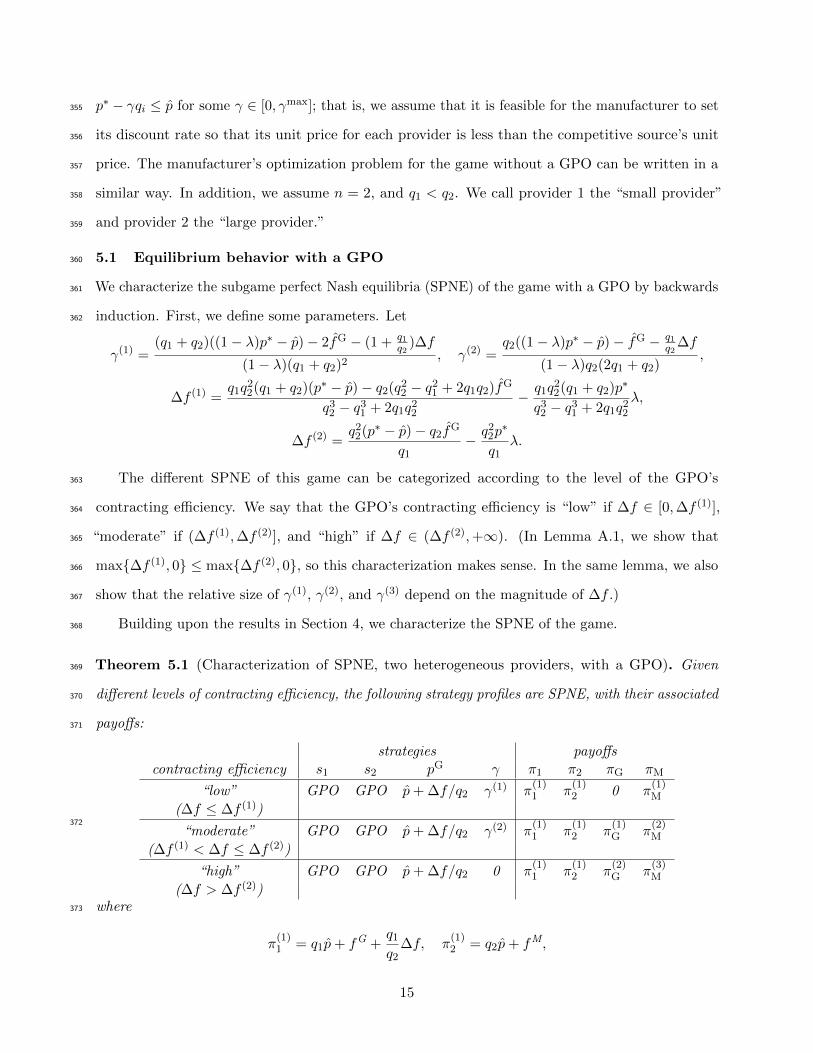
Theorem 5.1 (Characterization of SPNE, two heterogeneous providers, with a GPO). Given369
different levels of contracting efficiency, the following strategy profiles are SPNE, with their associated370
payoffs:371
strategies payoffscontracting efficiency s1 s2 pG γ π1 π2 πG πM
“low” GPO GPO p̂+ ∆f/q2 γ(1) π(1)1 π
(1)2 0 π
(1)M
(∆f ≤ ∆f (1))
“moderate” GPO GPO p̂+ ∆f/q2 γ(2) π(1)1 π
(1)2 π
(1)G π
(2)M
(∆f (1) < ∆f ≤ ∆f (2))
“high” GPO GPO p̂+ ∆f/q2 0 π(1)1 π
(1)2 π
(2)G π
(3)M
(∆f > ∆f (2))
372
where373
π(1)1 = q1p̂+ fG +
q1
q2∆f, π
(1)2 = q2p̂+ fM,
15

π(1)G =
q22 − q2
1 + 2q1q2
q2(2q1 + q2)f̂G +
q1(q1 + q2)
2q1 + q2
(p̂− (1− λ)p∗
)+
(q1 + q2)(q22 − q2
1 + q1q2)
q22(2q1 + q2)
∆f,
π(2)G = 2f̂G + (q1 + q2)
(p̂− (1− λ)p∗
)+(
1 +q1
q2
)∆f, π
(1)M = (q1 + q2)
(p̂+
∆f
q2
)+ 2f̂G,
π(2)M =
q1(q1 + q2)
2q1 + q2(1− λ)p∗ +
(q1 + q2)2
2q1 + q2
(p̂+
f̂G
q2+
∆f
q2
q1
q2
), π
(3)M = (1− λ)(q1 + q2)p∗.
Note that both providers always purchase from the GPO in equilibrium. This result generalizes374
to n > 2 providers with identical purchasing requirements (§6). However, this result does not apply375
in general. The price pG that the GPO charges is the breakeven price for the large provider. The376
small provider benefits from the magnitude of the large provider’s purchasing requirement: the total377
purchasing cost π1 of the small provider decreases as the large provider’s purchasing requirement q2378
increases. However, the large provider’s total purchasing cost π2 does not depend on the smaller379
provider’s purchasing requirement q1.380
Also we see that the GPO’s profit πG is strictly positive when the contracting efficiency is381
moderate or high. When its contracting efficiency is low, the manufacturer collects all the payments382
from providers, and the GPO just breaks even (i.e., πM = π1 +π2 and πG = 0). When the contracting383
efficiency is moderate or high, the GPO is no longer a profitless intermediary, and the payments384
from the providers are split between the manufacturer and the GPO (i.e., πM + πG = π1 + π2 and385
πG ≥ 0).386
The GPO membership fee affects the players in different ways. For all levels of contracting387
efficiency, we observe the following for a given value of the total fixed contracting cost fG. As the388
GPO membership fee f̂G increases, the GPO’s profit πG and the manufacturer’s profit πM stay the389
same or increase. However, the providers’ total purchasing costs π1 and π2 are not affected: the390
providers’ total fixed contracting cost fG remains the same, and a change in the membership fee391
only changes how much of fG gets transferred to the GPO.392
Interestingly, the manufacturer’s effective unit price for the small provider p∗ − γq1 and the393
large provider p∗ − γq2 is greater than the competitive source’s unit price p̂. In particular, the394
proof of Theorem 5.1 indicates that the manufacturer’s discount rate γ at equilibrium does not395
exceed (p∗ − p̂)/q2 and (p∗ − p̂)/q1. Despite this, the manufacturer still “gets the business” of the396
providers because of the GPO’s contracting efficiency and aggregating abilities. Also, note that397
when the GPO’s contracting efficiency is “high”, the manufacturer’s optimal strategy is to set a398
16

zero discount rate. In this regime, the GPO’s contracting efficiency is so large that both providers399
will purchase through the GPO, regardless of the manufacturer’s quantity-discount schedule, and so400
the manufacturer optimizes by not offering a discount at all.401
Next, we more closely examine the behavior of the equilibria described in Theorem 5.1 with402
respect to the contracting administration fee λ and the contracting efficiency ∆f . To facilitate the403
analysis, we define the following regions in (λ,∆f)-space:404
ΞL = {(λ,∆f) : 0 ≤ ∆f ≤ ∆f (1), 0 ≤ λ ≤ 1}, ΞM = {(λ,∆f) : ∆f (1) < ∆f ≤ ∆f (2), 0 ≤ λ ≤ 1},
ΞH = {(λ,∆f) : ∆f > ∆f (2), 0 ≤ λ ≤ 1}.
Figure 2 illustrates the characterization of SPNE described in Theorem 5.1 in (λ,∆f)-space. The405
providers’ costs, the GPO’s profit, and the manufacturer’s profit at equilibrium as functions of λ406
and ∆f are:407
π1(λ,∆f) = π(1)1 for all (λ,∆f) ∈ ΞL ∪ ΞM ∪ ΞH,
π2(λ,∆f) = π(1)2 for all (λ,∆f) ∈ ΞL ∪ ΞM ∪ ΞH,
πG(λ,∆f) =
0 if (λ,∆f) ∈ ΞL,
π(1)G if (λ,∆f) ∈ ΞM,
π(2)G if (λ,∆f) ∈ ΞH;
πM(λ,∆f) =
π
(1)M if (λ,∆f) ∈ ΞL,
π(2)M if (λ,∆f) ∈ ΞM,
π(3)M if (λ,∆f) ∈ ΞH.
In addition, in order to examine how the manufacturer and the GPO share the revenue coming from408
the providers, we define the profit share of the GPO as409
ρG =πG
πM + πG.
In the following corollary, we examine how these quantities behave as functions of the contracting410
efficiency, ∆f , and the CAF, λ. Recall that the providers’ total fixed contracting cost fG consists411
of f̂G, the GPO membership fee, and f̃G, the providers’ fixed contracting cost when purchasing412
through the GPO. With fM and f̂G fixed, an increase in the contracting efficiency ∆f = fM− fG =413
fM − f̂G − f̃G corresponds to a decrease in f̃G.414
Corollary 5.2. Suppose fM and f̂G are fixed. Then:415
17

λ
∆f
∆f (1)
∆f(2)
1
s1 = GPO
s2 = GPO
pG = p̂+ ∆f/q2, πG = 0
γ = γ(1)
ΞL
s1 = GPO
s2 = GPO
pG = p̂+ ∆f/q2, πG > 0
γ = γ(2)
ΞM s1 = GPO
s2 = GPO
pG = p̂+ ∆f/q2, πG > 0
γ = 0
ΞH
Figure 2: Characterization of the SPNE described in Theorem 5.1 in (λ,∆f)-space.
π1(λ,∆f) π2(λ,∆f) πG(λ,∆f) πM(λ,∆f) ρG
as a fn. nonincreasing, constant nondecreasing, nondecreasing, nondecreasingof ∆f linear piecewise linear, piecewise linear,
convex concave
as a fn. constant constant nondecreasing, nonincreasing, nondecreasingof λ piecewise linear, piecewise linear,
convex concave
416
First, Corollary 5.2 states that as the contracting efficiency increases, the small provider’s417
total purchasing cost decreases, while the large provider’s total purchasing cost stays the same.418
In addition, as the contracting efficiency increases, the profit of the GPO and the manufacturer419
increases. Therefore, an increase in contracting efficiency benefits all channel members. We expect420
this type of relationship for the GPO’s profit, since the GPO “charges” for the contracting efficiency421
in its unit on-contract price, as shown in Theorem 5.1. Interestingly, this “charge” for contracting422
efficiency trickles up to the manufacturer as well. This phenomenon is evidently attributable to the423
fact that the manufacturer anticipates the GPO’s response when determining its quantity-discount424
schedule, and as a result, is able to “capture” some of the GPO’s contracting efficiency.425
Next, consider the behavior of the equilibrium payoffs as the CAF varies. According to426
Corollary 5.2, neither provider’s total purchasing cost is affected by the CAF; the CAF only affects427
the profits of the GPO and the manufacturer. As the CAF increases, the GPO’s profit increases,428
while the manufacturer’s profit decreases. However, their total profits remain unchanged because429
the providers’ total costs are invariant to the CAFs. The higher the CAF, the more profitable the430
18

GPO. Finally, as both the contracting efficiency and the CAF increase, the GPO captures a larger431
fraction of the revenue collected from the providers.432
The top row of plots in Figure 5 (page 28) illustrates the behaviors described in Corollary 5.2 in433
(λ,∆f)-space. Note that lighter areas indicate lower values and darker areas, higher values. The434
diagonal lines in each plot are provided as a guide for comparison with Figure 2. Note that in the435
first two plots from the left, neither provider’s total purchasing cost is affected by the CAF (i.e., the436
plots do not change shading along any horizontal line). The large provider’s total purchasing cost is437
also unaffected by ∆f (i.e., the plot does not change shading along any vertical line). However, the438
small provider’s total purchasing cost is nonincreasing in ∆f (i.e., the shading in the plot lightens439
going up any vertical line). GPO and manufacturer profit are displayed in the third and fourth440
plots of the same row: note that the GPO’s profit is nondecreasing and the manufacturer’s profit is441
nonincreasing in the CAF. Both the GPO and the manufacturer’s profit is nondecreasing in ∆f . In442
the fifth plot, the GPO’s fraction of profit is nondecreasing in both λ and ∆f . As already noted, in443
the sixth plot, both providers always purchase through the GPO in this scenario.444
For more general cases (e.g., a nonlinear manufacturer quantity-discount schedule) we are unable445
to provide analytic results, but computational experiments indicate that provider total purchasing446
cost and GPO/manufacturer profit behave in a similar manner. See §7.447
5.2 Equilibrium behavior without a GPO448
Define p̂(1) = q2(q2−q1)q21+q2(q2−q1)
p∗. The different SPNE of this game can be described in terms of the449
level of competition between the manufacturer and the competitive source. We say there is “high”450
competition if p̂ ∈ [0, p̂(1)], and “low” competition if p̂ ∈ (p̂(1), p∗]. For the game without a GPO, we451
have the following characterization of SPNE.452
Theorem 5.3 (Characterization of SPNE, two heterogeneous providers, without a GPO). Given453
different levels of competition, the following strategy profiles are SPNE, with their associated payoffs:454
strategies payoffscompetition s1 s2 γ π1 π2 πM
“high” comp mfr (p∗ − p̂)/q2 π(2)1 π
(2)2 π
(4)M
(0 ≤ p̂ ≤ p̂(1))
“low” mfr mfr (p∗ − p̂)/q1 π(2)1 π
(3)2 π
(5)M
(p̂(1) < p̂ ≤ p∗)
455
19

where456
π(2)1 = q1p̂+ fM, π
(2)2 = q2p̂+ fM, π
(3)2 = q2
(q2
q1p̂−
(q2
q1− 1)p∗)
+ fM,
π(4)M = q2p̂, π
(5)M = q1p̂+ q2
(q2
q1p̂− (
q2
q1− 1)p∗
).
The equilibria described in Theorem 5.3 are driven by the usual trade-off between price and457
volume. When competition is low, the competitive source’s unit price is relatively high. So in this458
scenario, the manufacturer can easily provide a unit price to both providers that is lower than the459
competitive source’s, by setting a relatively low discount rate. On the other hand, when competition460
is higher, the competitive source’s unit price is relatively low. So, in order to compete with the461
competitive source for both providers, the manufacturer must set a relatively high discount rate. As462
a result of the trade-off between price and volume, the manufacturer may find it more profitable to463
attract only the large provider.464
5.3 The effect of a GPO’s presence465
The presence of a GPO affects the total purchasing cost of the providers in different ways. These466
differences are partly driven by the mechanisms that the manufacturer and the GPO use to price467
the product. Lemma 4.2 tells us that when it is optimal for the large provider to purchase through468
the GPO, it is optimal for the smaller provider as well. The opposite holds for purchasing from the469
manufacturer.470
Comparing the equilibrium total purchasing costs of the providers with and without the presence471
of the GPO, we obtain the following corollary.472
Corollary 5.4. (a) π(1)1 < π
(2)1 ; (b) π
(1)2 = π
(2)2 > π
(3)2 .473
We see that the small provider benefits from the presence of the GPO: its total purchasing cost in474
the presence of a GPO is always strictly less than its total purchasing cost in the absence of a GPO.475
However, the large provider benefits from the absence of a GPO: its total purchasing cost in the476
absence of a GPO is no greater than that in the presence of a GPO. Moreover, when there is “low”477
competition, its total purchasing cost in the absence of a GPO is strictly less. This occurs since in478
the absence of a GPO, the large provider benefits when the manufacturer sets a higher discount479
rate in order to attract the small provider.480
As discussed above, the providers face a higher unit price in the presence of a GPO. In the481
20
absence of a GPO, the effective unit price to the providers is p̂, while in the presence of a GPO,482
the effective unit price to the providers is p̂+ ∆f/qi. However, this difference is offset by the lower483
contracting costs in the presence of a GPO. This result is consistent with the findings of a pilot484
study described in §2: that GPO prices were not always lower but often higher than prices paid485
by providers that negotiated directly with vendors. These GAO findings are used as criticisms of486
GPOs. However, as shown in our model, this result is consistent with providers seeking the lowest487
total purchasing cost but not necessarily the lowest unit cost.488
In the absence of a GPO, the manufacturer may not be able to attract the business of both489
providers, while in the presence of a GPO, the manufacturer gets the business of both providers490
through the GPO. This occurs when competition is sufficiently high; that is, when the base unit491
price p∗ and the competitive source’s unit price p̂ are so far apart that the manufacturer is unable492
to set a sufficiently high discount rate to compete with the competitive source.493
6 The case of n identical providers and linear quantity discount494
We now focus on the case with n identical providers, i.e, q1 = · · · = qn = q and a linear quantity-495
discount schedule. By symmetry, all n providers have the same equilibrium strategy and associated496
payoff. We denote this strategy simply by si and the associated payoff πi.497
First, we consider the equilibrium behavior in the game with a GPO. Define498
γ(3) =q(p∗ − p̂)− f̂G −∆f
(1− λ)nq2− p∗
(1− λ)nqλ, ∆f (3) = q(p∗ − p̂)− f̂G − λqp∗.
In this case, we say that the GPO’s contracting efficiency is “low” if ∆f ∈ [0,∆f (3)], and “high” if499
∆f ∈ (∆f (3),+∞). Intuitively, at equilibrium, the manufacturer and the GPO set prices to extract500
as much profit as possible from the providers, since the providers are identical. This reasoning501
results in the following theorem.502
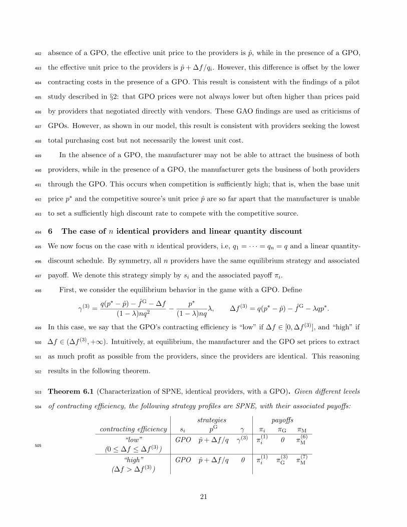
Theorem 6.1 (Characterization of SPNE, identical providers, with a GPO). Given different levels503
of contracting efficiency, the following strategy profiles are SPNE, with their associated payoffs:504
strategies payoffscontracting efficiency si pG γ πi πG πM
“low” GPO p̂+ ∆f/q γ(3) π(1)i 0 π
(6)M
(0 ≤ ∆f ≤ ∆f (3))
“high” GPO p̂+ ∆f/q 0 π(1)i π
(3)G π
(7)M
(∆f > ∆f (3))
505
21

λ
∆f
∆f (3)
1
si = GPO
pG = p̂+ ∆f/q, πG = 0
γ = γ(3)
ΞL
si = GPO
pG = p̂+ ∆f/q, πG > 0
γ = 0
ΞH
Figure 3: Characterization of the SPNE described in Theorem 6.1 in (λ,∆f)-space.
where506
π(1)i = qp̂+ fM, π
(3)G = nq
(p̂− (1− λ)p∗
)+ nf̂G + n∆f,
π(6)M = nqp̂+ nf̂G + n∆f, π
(7)M = (1− λ)nqp∗.
The managerial interpretations for the equilibrium behavior in the case of two heterogeneous507
providers discussed in §5.1 hold in this case of n identical providers as well.508
As before, we define regions of “low” and “high” contracting efficiency in (λ,∆f)-space:509
ΞL = {(λ,∆f) : 0 ≤ ∆f ≤ ∆f (3), 0 ≤ λ ≤ 1}, ΞH = {(λ,∆f) : ∆f > ∆f (3), 0 ≤ λ ≤ 1}.
Figure 3 illustrates the characterization of SPNE described in Theorem 6.1 in (λ,∆f)-space. The510
providers’ costs, the GPO’s profit, and the manufacturer’s profit at equilibrium as functions of λ511
and ∆f are:512
πi(λ,∆f) = π(1)i for all (λ,∆f) ∈ ΞL ∪ ΞH,
πG(λ,∆f) =
0 if (λ,∆f) ∈ ΞL,
π(3)G if (λ,∆f) ∈ ΞH;
πM(λ,∆f) =
π
(6)M if (λ,∆f) ∈ ΞL,
π(7)M if (λ,∆f) ∈ ΞH.
We also look at the GPO’s profit share ρG as a function of λ and ∆f .513
Corollary 6.2. Suppose fM and f̂G are fixed. Then:514
22

πi(λ,∆f) πG(λ,∆f) πM(λ,∆f) ρG
as a fn. constant nondecreasing, nondecreasing, nondecreasingof ∆f piecewise linear, piecewise linear,
convex concave
as a fn. constant nondecreasing, nonincreasing, nondecreasingof λ piecewise linear, piecewise linear,
convex concave
515
These behaviors are qualitatively identical to the case of two heterogeneous providers. The516
top row of plots in Figure 6 (page 28) illustrate the results of Corollary 6.2 in (λ,∆f)-space. The517
diagonal lines in each plot are provided as a guide for comparison with Figure 3. As before, lighter518
areas indicate smaller values and darker areas, larger values. Comparing the shading in the top row519
of Figure 6 with that of Figure 5, we see that the results are quite similar.520
Now we turn to equilibrium behavior in the game without a GPO. Using Lemma 4.4, we have521
the following characterization of subgame perfect Nash equilibrium.522
Theorem 6.3 (Characterization of SPNE, identical providers, without a GPO). The strategy profile523
si = mfr, γ = p∗−p̂q is an SPNE, with associated payoffs πi = qp̂+ fM and πM = nqp̂.524
As in the case of two heterogeneous providers, the equilibria described in Theorem 6.3 are525
largely driven by the usual trade-off between price and volume. Like the case of two heterogeneous526
providers, the providers face a higher unit price in the presence of a GPO, which is offset by the527
lower contracting costs in the presence of a GPO.528
7 Returning to more general cases529
In this section, we identify equilibrium behaviors from §5 and §6 that appear to extend to more530
general cases: n providers with arbitrary fixed purchasing requirements and a manufacturer’s531
quantity-discount schedule that is nonlinear.532
7.1 The case of n providers with arbitrary purchasing requirements and linear quan-533
tity discount534
Given that all of the providers buy through the GPO in the two special cases examined above (both535
with a linear quantity-discount schedule), we decided to examine the scenario with n heterogeneous536
providers and a linear quantity-discount schedule, partly to see if the “all-providers-buy-through-537
the-GPO” result was an artifact of our model, but more importantly, to see if other characteristics538
of the equilibria in these special cases continued to apply in this more general scenario.539
23

0
20
40
∆f
sum of allproviders’ totalpurchasing costs GPO profit πG
manufacturerprofit πM
GPO profitshare ρG
fraction ofproviders buying
through GPO
0
20
40
∆f
0.1 0.3 0.50
20
40
λ
∆f
500 900
0.1 0.3 0.5
λ
0 800
0.1 0.3 0.5
λ
0 700
0.1 0.3 0.5
λ
0 1
0.1 0.3 0.5
λ
0 1
identicalq1 = · · · = q10 = 4.5
almost identicalq1 = · · · = q5 = 4
q6 = · · · = q10 = 5
highly varying
q1 = · · · = q5 = 1
q6 = · · · = q8 = 4
q9 = q10 = 14
Figure 4: Comparison of equilibrium behavior with 10 providers under different purchasing requirementdistributions, with a linear quantity discount schedule. Here, n = 10, p∗ = 16, p̂ = 8, f̂G = 1, fM = 50.
Although we are unable to obtain closed-form expressions for equilibrium strategies and payoffs540
in this case, we computed them for a variety of parameterizations, using the procedure described541
in §4. We discretized the space of linear quantity-discount schedules p(q) = p∗ − γq by restricting542
the domain of γ to 1,000 uniformly spaced values in [0, γmax]. Using this discretization of the543
quantity-discount schedule, we computed approximate SPNEs for 2,500 uniformly spaced points in544
the (λ,∆f)-space, where λ ∈ [0, 1/2] and ∆f ∈ [0, fM − f̂G]. In this paper, we only show results for545
λ ∈ [0, 1/2], since values of the CAF λ are typically closer to 0 than 1.546
Compare the top row of Figure 4, which shows the equilibrium behavior of an instance of547
the identical-provider case (from §6), and the middle row, which shows the equilibrium behavior548
of an instance of the “almost-identical-providers” case. (In both instances, the total provider549
requirement equals 45.) Note that in the “almost-identical-providers” case, all of the providers550
purchase their requirements through the GPO in equilibrium, just like in the identical-provider case.551
In addition, the influence of λ and ∆f on GPO and manufacturer profit, and GPO profit share552
in this “almost-identical provider” case are the same as those in the identical-provider case. For553
example, in both cases, the GPO’s profit is nondecreasing in λ and ∆f , while the manufacturer’s554
profit is nonincreasing in λ and nondecreasing in ∆f .555
24

On the other hand, a large variance in the providers’ purchasing requirements provides the556
GPO the opportunity to maximize its profit by setting its price so that it attracts only the smallest557
providers. The bottom row of Figure 4 displays the equilibrium behavior of 10 providers with highly558
varying purchasing requirements. (Again, the total provider requirement equals 45.) As shown in559
the last plot of the bottom row, not all the providers buy through the GPO; instead, providers 6560
through 10—the providers with the five largest purchasing requirements—buy directly from the561
competitive source when the GPO’s contracting efficiency is high and the CAF is low (the upper-left562
of the plot) while the providers with smaller purchasing requirements buy through the GPO. Note563
in the other plots on the bottom row of Figure 4, that this same region of (λ,∆f)-space provides564
relatively higher profits to the GPO and relatively much lower profits to the manufacturer.565
These observations are intuitive. When the providers are relatively homogeneous, they each566
benefit similarly from the aggregation ability of the GPO. In addition, the homogeneity of the567
purchasing requirements diminishes the effect of GPO’s tradeoff between its unit on-contract price568
and volume. However, when the providers are relatively heterogeneous, they benefit differently from569
the aggregating ability of the GPO. Also, when the GPO’s contracting efficiency is high, the GPO570
is in a position to attract virtually any provider that it chooses to. Hence, its profit-maximizing571
price does not necessarily attract the largest providers.572
The following theorem provides sufficient conditions for this observed behavior in the general case:573
n providers with arbitrary purchasing requirements and a generic manufacturer’s quanitty-discount574
schedule p(·) such that p(q) is nonincreasing in q and the associated revenue p(q)q is nondecreasing575
in q.576
Theorem 7.1. Suppose n ≥ 3. In addition, suppose there exists a constant M independent of577
∆f such that for any p(·) that is feasible for the manufacturer, 0 ≤ p(q) ≤ M for all q ≥ 0. Let578
k′ = min{k : qk+1 = · · · = qn}. If579
1
qn
n−1∑i=1
qi −1
qk′
k′−1∑i=1
qi < 0, (7.1)
then for sufficiently high ∆f , there exist providers that do not purchase through the GPO in580
equilibrium.581
In particular, Theorem 7.1 holds when the manufacturer’s quantity-discount schedule is linear—582
that is, of the form (5.1). In this case, since the manufacturer’s choice of discount rate γ is583
25

constrained between 0 and γmax = p∗/(2∑n
i=1 qi), the unit price p(q) is bounded, independent of584
∆f . Note also that (7.1) can never hold when n = 2 or with n identical providers.585
In summary, in the limited number of instances we observed, the qualitative results for scenarios586
with 2 heterogeneous providers (§5) and n identical providers (§6) appear to apply to scenarios587
with n similar, but heterogeneous providers. When there are many providers with highly varying588
purchasing requirements, all providers no longer necessarily purchase through the GPO.589
7.2 Linear vs. nonlinear quantity-discount schedules590
In §5 and §6, we studied games where the manufacturer announces a linear quantity-discount schedule591
of the form (5.1). Now suppose that the manufacturer announces a nonlinear quantity-discount592
schedule of the following form:593
p(q) = p̃+η
qγ. (7.2)
Schotanus et al. (2009) proposed this functional form, tested its fit using “actual offers provided to594
purchasing groups, and internet stores,” and reported that this functional form “fits very well with595
almost all quantity discount schedule types” they examined. As before, the manufacturer’s decision596
variable is γ. Note that when η > 0, the quantity-discount schedule p(q) is nonincreasing in q for all597
q if and only if γ ≥ 0, and the associated revenue p(q)q is nondecreasing in q for all q ∈ [0,∑n
i=1 qi]598
if and only if γ ∈ [0, 1]. On the other hand, when η < 0, the quantity-discount schedule p(q) is599
nonincreasing in q for all q if and only if γ ≤ 0. In this case, there exists some γmin ∈ (−∞, 0]600
such that the associated revenue p(q)q is nondecreasing in q for all q ∈ [0,∑n
i=1 qi] if and only if601
γ ∈ [γmin, 0].602
Although we are unable to obtain a closed-form characterization of the equilibrium strategies603
and payoffs when the quantity-discount schedule is of the form (7.2), the equilibria can be computed604
numerically, using the procedure described in §4. For these computations, we fixed the value of η,605
and discretized the space of nonlinear quantity-discount schedules by restricting the domain of γ.606
When η > 0, we restricted the domain of γ to 1,000 uniformly spaced values in [0, 1]. When η < 0,607
we computed the value of γmin (described above), and restricted the domain of γ to 1,000 uniformly608
spaced values in [γmin, 0]. Using this discretization of the quantity-discount schedules, we computed609
approximate SPNEs for 2,500 uniformly spaced points in the (λ,∆f)-space, where λ ∈ [0, 1] and610
∆f ∈ [0, fM − f̂G].611
26

Through these computational experiments, we observed that in both the case of two heterogeneous612
providers and the case of n identical providers, the game with the nonlinear quantity-discount613
schedule appears to exhibit the same properties as we observed in the game with the linear614
quantity-discount schedule. In particular, the qualitative attributes in Corollaries 5.2 and 6.2615
match. To illustrate: Figure 5 shows the equilibrium behavior for an instance of the game with two616
heterogeneous providers, under a linear quantity-discount schedule (with p∗ = 16) and two different617
nonlinear quantity-discount schedules (one with p̃ = 0 and η = 16, and the other with p̃ = 16 and618
η = −2). Figure 6 shows the equilibrium behavior for an instance with 10 identical providers, again619
under a linear and two different nonlinear quantity-discount schedules. Figure 7 shows a comparison620
of the quantity-discount schedules used in these examples.621
Note that the quantity-discount schedules used in these examples are similar, especially in622
their general behavior (nonincreasing, convex) and range. One might expect that similar sets of623
available quantity-discount schedules will yield similar equilibrium behavior regardless of the specific624
functional forms, as we have observed. This apparent robustness to the specific functional form625
might also be explained by the structural results in Lemmas 4.1-4.3, which hold for any quantity626
discount function that is nonincreasing in quantity and has nondecreasing associated revenue. This627
includes, for example, stepwise quantity discount functions, which Schotanus et al. (2009) fit using628
functions of the form (7.2).629
In summary, for scenarios with (1) n similar but heterogeneous providers facing a linear quantity-630
discount schedule, (2) two heterogeneous providers facing a nonlinear quantity-discount schedule, and631
(3) n identical providers facing a nonlinear quantity-discount schedule, we observe computationally632
that the behavior of the players’ equilibrium payoffs/costs with respect to λ and ∆f are similar to633
those proven for the scenarios with two heterogeneous providers and n identical providers, facing a634
linear quantity-discount schedule (§5 and §6). Based on this empirical evidence, and the general635
structural results governing equilibria in Lemmas 4.1-4.3, we conjecture that the results describing636
the behavior of the players’ equilibrium payoffs/costs with respect to λ and ∆f can be generalized637
beyond the cases studied in §5 and §6. Of course, this is only a conjecture, and proof of this638
conjecture requires further research.639
27

0
20
40
∆f
small providertotal purchasing
cost π1
large providertotal purchasing
cost π2 GPO profit πG
manufacturerprofit πM
GPO profitshare ρG
fraction ofproviders buying
through GPO
0
20
40
∆f
0.1 0.3 0.50
20
40
λ
∆f
70 80
0.1 0.3 0.5
λ
80 100
0.1 0.3 0.5
λ
0
0.1 0.3 0.5
λ
130
0.1 0.3 0.5
λ
0
0.1 0.3 0.5
λ
0 1
linearp∗ = 16
nonlinearp̃ = 0,
η = 16
nonlinearp̃ = 16,
η = −2
Figure 5: Comparison of equilibrium behavior under different quantity discount schedules, in the case of twoheterogeneous providers. Here, n = 2, q1 = 4, q2 = 5, p̂ = 8, f̂G = 1, fM = 50.
0
20
40
∆f
provider totalpurchasing cost
πi GPO profit πG
manufacturerprofit πM
GPO profitshare ρG
fraction ofproviders buying
through GPO
0
20
40
∆f
0.1 0.3 0.50
20
40
λ
∆f
80 90
0.1 0.3 0.5
λ
0 650
0.1 0.3 0.5
λ
0 500
0.1 0.3 0.5
λ
0 1
0.1 0.3 0.5
λ
0 1
linearp∗ = 16
nonlinearp̃ = 0,
η = 16
nonlinearp̃ = 16,
η = −2
Figure 6: Comparison of equilibrium behavior under different quantity discount schedules, in the case of 10identical providers. Here, n = 10, q1 = · · · = q10 = 4.5, p̂ = 8, f̂G = 1, fM = 50.
28

10 20 30 405
10
15
q
p(q)
|γ| = 0.04
10 20 30 40
q
|γ| = 0.08
10 20 30 40
q
|γ| = 0.12
10 20 30 40
q
|γ| = 0.16
linear nonlinear p̃ = 0, η = 16 nonlinear p̃ = 16, η = −2
Figure 7: Comparison of quantity discount functions.
8 Concluding remarks640
In this section, we answer the five questions posed in the introduction, adding a few suggestions for641
future research. Before doing so, we acknowledge that our model, and, hence, our results is/are642
limited to a scenario in which provider demand is inelastic (i.e., fixed provider requirements). Our643
model is also limited to a single product, whereas GPO pricing sometimes involves bundles of644
products. These extensions are worthy of future research. We will comment on the impact of other645
model assumptions below.646
Do providers experience lower prices or lower total purchasing costs with a GPO in the supply647
chain? Based on Lemma 4.2, in the general case, the GPO will set its price to be equal to the648
breakeven price—the price that equalizes the total purchasing cost—of the largest provider that649
it chooses to contract for (i.e., at the price that will maximize the GPO’s profit). Providers with650
smaller purchasing requirements will experience lower total purchasing costs in the presence of a651
GPO, but may experience higher per-unit prices.652
These answers must be carefully interpreted when provider-members share in GPO profits. Our653
model could be modified to account for this by including such profit-sharing in each provider’s654
total purchasing costs, and therefore each provider’s breakeven price. This, and the fact that large655
providers are more likely to be GPO owners, would increase the likelihood that larger providers will656
purchase through the GPO. This is a topic worthy of future research. Large providers may also657
demand that the GPO share its CAF. In effect, this would decrease such providers’ per unit cost658
and increase the likelihood of their purchases through the GPO. This, too, deserves more study.659
Do CAFs mean higher prices paid by providers? In the two special cases examined, the total660
29

purchasing cost of the providers is not affected by the CAF, although providers may experience661
higher unit prices. Based on computational experiments, it seems that this behavior occurs in more662
general cases as well. Interestingly, this matches one of the conclusions of Hu and Schwarz (2011).663
How does the presence of the GPO affect manufacturer profits? As displayed in all the cases664
examined, the manufacturer’s profit either does not change or decreases as the GPO’s CAF increases.665
In addition, the manufacturer’s profit and profit share either does not change or increases as the666
GPO’s contracting efficiency increases. Thus, the manufacturer benefits partially from the GPO’s667
contracting efficiency. Computational experiments indicate that this occurs in other cases as well.668
What affects GPO profits? In the special cases examined, we have demonstrated that GPO profit669
either does not change or increases as the CAF increases and as the GPO’s contracting efficiency670
decreases. Indeed, for low values of these parameters the GPO makes no profit. It appears that671
the same behavior holds for more general cases, based on computational tests. In contrast to the672
non-profit-maximizing GPO studied in Hu and Schwarz (2011), we show that the profit-maximizing673
GPO in our model does make a profit in some cases.674
Recall that in our model, the GPO’s contracting efficiency is net of the provider’s membership675
fee; i.e., the higher the membership fee, the lower the GPO’s contracting efficiency. Note that GPO676
membership fees may be different for smaller versus larger providers. Our model could be modified677
to account for this by adjusting each provider’s membership fee, and therefore each provider’s678
breakeven price accordingly. This, too, is a topic for future research.679
How are supply-chain profits divided between the manufacturer and the GPO and how is this680
influenced by the “power” of the GPO? As displayed in all cases examined, the GPO’s share of681
supply-chain profits increases or remains the same as either the CAF or the GPO’s contracting682
efficiency increases. The more powerful the GPO is in negotiating its CAF, and the more efficient it683
is, the higher its profit and its share of total supply-chain profit.684
References685
U. Arnold. 1997. Purchasing consortia as a strategic weapon for highly decentralized multi-divisional686
companies. In Proceedings of the 6th IPSERA Conference, pp. T3/7–1–T3/7–12. University of687
Naples Frederico II, Naples, Italy.688
L. R. Burns. 2002. The Health Care Value Chain: Producers, Purchasers, and Providers. Jossey-Bass.689
30

L. R. Burns, J. A. Lee. 2008. Hospital purchasing alliances: Utilization, services, and performance.690
Health Care Management Review 33:203–215.691
G. Cachon. 2003. Supply chain coordination with contracts. In S. Graves, T. de Kok, eds., Handbooks692
in Operations Research and Management Science: Supply Chain Management. Elsevier.693
R. R. Chen, P. Roma. 2008. Group-buying of competing retailers. Working paper. University of694
California at Davis.695
J. Dana. 2003. Buyer groups as strategic commitments. Working paper. Northwestern University.696
Q. Hu, L. Schwarz. 2011. Controversial role of GPOs in healthcare-product supply chains. Production697
and Operations Management 20:1–15.698
H. P. Marvel, H. Yang. 2008. Group purchasing, nonlinear tariffs, and oligopoly. International699
Journal of Industrial Organization 26:1090–1105.700
M. Nagarajan, G. Sosic, H. Zhang. 2008. Stability of group purchasing organization. Working paper.701
University of Southern California.702
D. P. O’Brien, G. Shaffer. 1997. Nonlinear supply contracts, exclusive dealing, and equilibrium703
market foreclosure. Journal of Economics & Management Strategy 64:755–785.704
E. S. Schneller, L. R. Smeltzer. 2006. Strategic Management of the Health Care Supply Chain. John705
Wiley and Sons.706
F. Schotanus, J. Telgen, L. de Boer. 2008. Unfair allocation of gains under equal price allocation707
method in purchasing groups. European Journal of Operations Research 187:162–176.708
F. Schotanus, J. Telgen, L. de Boer. 2009. Unraveling quantity discounts. Omega 37:510–521.709
S. P. Sethi. 2006. Group purchasing organizations: An evaluation of their effectiveness in provid-710
ing services to hospitals and their patients. Report No. ICCA-2006.G-01. URL: www.ICCA-711
corporatedaccountability.org.712
H. Singer. 2006. The budgetary impact of eliminating the gpo’s safe harbor exemption from the713
anti-kickback statute of the social security act. URL: www.criterioneconomics.com/pub.714
31

U.S. Government Accountability Office. 2002. Group purchasing organizations: pilot study suggests715
large buying groups do not always offer hospital lower prices. GAO Report GAO-02-690T.716
Testimony before the Subcommittee on Antitrust, Competition, and Business and Consumer717
Rights, Committee on the Judiciary, U.S. Senate, April 30, 2002.718
U.S. Government Accountability Office. 2003. Group purchasing organizations: use of contracting719
processes and strategies to award contracts for medical-surgical products. GAO Report GAO-720
03-998T. Testimony before the Subcommittee on Antitrust, Competition Policy and Consumer721
Rights, Committee on the Judiciary, U. S. Senate, July 16, 2003.722
U.S. Government Accountability Office. 2010. Group purchasing organizations: services provided to723
customers and initiatives regarding their business practices. GAO Report GAO-10-738. Report to724
the Ranking Member, Committee on Finance, U.S. Senate, August 2010.725
U.S. Senate Minority Staff Report. 2010. Empirical data lacking to support claims of savings with726
group purchasing organizations. 111th U.S. Congress, Senate Finance Committee, September 24,727
2010.728
Y. Wang, L. Jiang, Z. J. Shen. 2004. Channel performance under consignment contract with revenue729
sharing. Management Science 50:34–37.730
32

A Proofs731
We abuse notation and let πG(pG) denote the GPO’s profit as a function of its unit price pG, and732
let πM(γ) denote the manufacturer’s revenue as a function of its discount rate γ.733
A.1 Section 4734
Proof of Lemma 4.1. Consider provider i ∈ {1, . . . , n}. Suppose provider i purchases non-zero735
quantities from all of its three options. In particular, suppose provider i purchases βGqi through736
the GPO, βMqi from the manufacturer, and (1− βG − βM)qi from the competitive source, for some737
βG, βM ∈ (0, 1) such that βG + βM < 1. Then, provider i’s total purchasing cost is738
fG+βGqipG + fM + βMqi(p
∗ − γβMqi) + fM + (1− βG − βMqip̂)
≥ βG(fG + qipG) + βM(fM + qi(p
∗ − γqi)) + (1− βG − βM)(fM + qip̂)
≥ min{fG + qipG, fM + qi(p
∗ − γqi), fM + qip̂}.
The first inequality holds since fG ≥ 0, fM ≥ 0, pG ≥ 0, p̂ ≥ 0, and p(βMqi) ≥ p(qi). As a result, it739
is clear that for fixed values of pG and γ, it is optimal for provider i to purchase its entire requirement740
from the option that offers the lowest total cost. The lemma follows from this observation.741
Proof of Lemma 4.2. Recall that we assume q1 ≤ · · · ≤ qn without loss of generality. Suppose pG is742
an optimal strategy for the GPO, such that pG ≤ min{p(qk), p̂}+ ∆fqk
for some k that satisfies qk < qj743
for all j = k + 1, . . . , n. Then, by Lemma 4.1, providers 1, . . . , k purchase their entire requirement744
through the GPO, and the GPO’s profit is kf̂G + pG∑k
i=1 qi − (1− λ)p(∑k
j=1 qj)∑k
i=1 qi. Since pG745
is optimal, it must be that pG = min{p(qk), p̂}+ ∆fqk
. Note that if pG = +∞, then the GPO’s profit746
is 0. The claim follows.747
Proof of Lemma 4.3. This follows as a consequence of Lemma 4.2 and backwards induction.748
Proof of Lemma 4.4. Similar to proof of Lemma 4.1.749
Proof of Lemma 4.5. This follows as a consequence of Lemma 4.4 and backwards induction.750
A.2 Section 5751
Before we begin, we show some properties of ∆f (1), ∆f (2), γ(0), γ(1), and γ(2), where752
γ(0) =q1((1− λ)p∗ − p̂)− f̂G −∆f
(1− λ)q21
.
A-1

Lemma A.1. (a) max{∆f (1), 0} ≤ max{∆f (2), 0} for any λ ∈ [0, 1]; (b) If ∆f ≤ ∆f (1), then753
γ(0) ≥ γ(1) ≥ γ(2); (c) If ∆f > ∆f (1), then γ(0) < γ(1) < γ(2); (d) If 0 ≤ ∆f ≤ max{0,∆f (1)}, then754
γ(1) ≥ 0; (e) ∆f ≤ ∆f (2) if and only if γ(2) ≥ 0; (f) γ(1) ≤ p∗−p̂q2
; (g) γ(2) ≤ p∗−p̂q2
.755
Proof. First, we show part a. Let756
λ(1) =p∗ − p̂p∗
− f̂G
p∗q2
2 − q21 + 2q1q2
q1q2(q1 + q2)and λ(2) =
p∗ − p̂p∗
− f̂G
p∗1
q2.
Note that ∆f (1) ≥ 0 when λ ≤ λ(1), and ∆f (2) ≥ 0 when λ ≤ λ(2). We have that λ(2) ≥ λ(1), since757
λ(2) − λ(1) =f̂G
p∗(q2
2 − q21 + 2q1q2
q1q2(q1 + q2)− 1
q2
)=
f̂G
p∗q2
q2(q2 − q1)
q1(q1 + q2)≥ 0.
Therefore, for all λ ∈ [λ(1), 1], the claim holds. Note that758
∆f (1) =q1q
22(q1 + q2)
q32 − q3
1 + 2q1q22
(λ(1) − λ) and ∆f (2) ≥ q22
q1(λ(1) − λ).
Since759
q22
q1− q1q
22(q1 + q2)
q32 − q3
1 + 2q1q22
=q2
2(q32 − q3
1 + 2q1q22)− q2
1q22(q1 + q2)
q1(q32 − q3
1 + 2q1q22)
=q2
2(q32 − q3
1 + q1(2q22 − q2
1 − q1q2))
q1(q32 − q3
1 + 2q1q22)
≥ 0,
for any λ ∈ [0, λ(1)], the claim also holds.760
Now, we show part b. Since ∆f ≤ ∆f (1), we have that761
γ(0) − γ(1) =q1q
22(q1 + q2)((1− λ)p∗ − p̂)− q2(q2
2 − q21 + 2q1q2)f̂G −∆f(q3
2 − q31 + 2q1q
22)
(1− λ)q21(q1 + q2)2
≥ 0,
γ(1) − γ(2) =q2(q1 + q2)(2q1 + q2)((1− λ)p∗ − p̂)− 2q1(2q1 + q2)f̂G −∆f(1 + q1
q2)q2(2q1 + q2)
(1− λ)q2(q1 + q2)2(2q1 + q2)
−q2(q1 + q2)2((1− λ)p∗ − p̂)− (q1 + q2)2f̂G −∆f q1q2 (q1 + q2)2
(1− λ)q2(q1 + q2)2(2q1 + q2)≥ 0.
Part c follows in a similar manner.762
Next, we show part d.763
γ(1) =(q1 + q2)((1− λ)p∗ − p̂)− 2f̂G −∆f(1 + q1
q2)
(1− λ)(q1 + q2)2
(i)
≥ q2(q1 + q2)(q22 − q2
1)((q1 + q2)(p∗ − p̂)− (q1 + q2)p∗λ− f̂G)
(1− λ)(q1 + q2)2(q32 − q3
1 + 2q1q2)
(ii)
≥ (q1 + q2)(q22 − q2
1)(q22 − q2
1 + q1q2)
(1− λ)q1q2(q1 + q2)2(q32 − q3
1 + 2q1q2)≥ 0.
Above, inequality (i) holds since ∆f ≤ ∆f (1), and inequality (ii) holds since λ ≤ λ(1).764
A-2
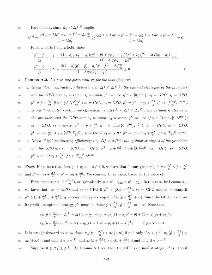
Part e holds, since ∆f ≤ ∆f (2) implies765
γ(2) =q2((1− λ)p∗ − p̂)− f̂G −∆f q1q2
(1− λ)q21
≥ q2((1− λ)p∗ − p̂)− f̂G − q2((1− λ)p∗ − p̂) + f̂G
(1− λ)q21
= 0.
Finally, parts f and g hold, since766
p∗ − p̂q2
− γ(1) =(1− λ)q1(q1 + q2)(p∗ − p̂) + q2(q1 + q2)λp∗ + 2q2f̂
G + ∆f(q1 + q2)
(1− λ)q2(q1 + q2)2≥ 0,
p∗ − p̂q2
− γ(2) =2(1− λ)(p∗ − p̂) + q2λp̂+ f̂G + ∆f q1q2
(1− λ)q2(2q1 + q2)≥ 0.
Lemma A.2. Let γ be any given strategy for the manufacturer.767
a. Given “low” contracting efficiency; i.e., ∆f ≤ ∆f (1): the optimal strategies of the providers768
and the GPO are: s1 = comp, s2 = comp, pG = +∞ if γ ∈ [0, γ(1)); s1 = GPO, s2 = GPO,769
pG = p̂+ ∆fq2
if γ ∈ [γ(1), p∗−p̂q2
); s1 = GPO, s2 = GPO, pG = p∗ − γq2 + ∆fq2
if γ ∈ [p∗−p̂q2
, γmax].770
b. Given “moderate” contracting efficiency; i.e., ∆f (1) < ∆f ≤ ∆f (2): the optimal strategies of771
the providers and the GPO are: s1 = comp, s2 = comp, pG = +∞ if γ ∈ [0,max{0, γ(0)});772
s1 = GPO, s2 = comp, pG = p̂ + ∆fq1
if γ ∈ [max{0, γ(0)}, γ(2)); s1 = GPO, s2 = GPO,773
pG = p̂+ ∆fq2
if γ ∈ [γ(2), p∗−p̂q2
); s1 = GPO, s2 = GPO, pG = p∗ − γq2 + ∆fq2
if γ ∈ [p∗−p̂q2
, γmax].774
c. Given “high” contracting efficiency; i.e., ∆f > ∆f (2): the optimal strategies of the providers775
and the GPO are s1 = GPO, s2 = GPO, pG = p̂+ ∆fq2
if γ ∈ [0, p∗−p̂q2
); s1 = GPO, s2 = GPO,776
pG = p∗ − γq2 + ∆fq2
if γ ∈ [p∗−p̂q2
, γmax].777
Proof. First, note that since q1 < q2 and ∆f > 0, we have that for any given γ ≥ 0, p̂+ ∆fq2< p̂+ ∆f
q1778
and p∗ − γq2 + ∆fq2< p∗ − γq1 + ∆f
q1. We consider three cases, based on the value of γ.779
First, suppose γ ∈ [0, p∗−p̂q2
), or equivalently, p̂ < p∗−γq2 < p∗−γq1. In this case, by Lemma 4.1,780
we have that: s1 = GPO and s2 = GPO if pG ∈ [0, p̂ + ∆fq2
]; s1 = GPO and s2 = comp if781
pG ∈ (p̂+ ∆fq2, p̂+ ∆f
q1]; s1 = comp and s2 = comp if pG ∈ (p̂+ ∆f
q1,+∞). Since the GPO maximizes782
its profit, its optimal strategy pG must be either p̂+ ∆fq2
, p̂+ ∆fq1
, or +∞. Note that783
πG(p̂+ ∆fq2
) = 2f̂G + ∆f(1 + q1q2
)− (q1 + q2)((1− λ)p∗ − p̂) + (1− λ)(q1 + q2)2γ,
πG(p̂+ ∆fq1
) = f̂G + ∆f − q1((1− λ)p∗ − p̂) + (1− λ)q21γ, πG(+∞) = 0.
It is straightforward to show that: πG(p̂+ ∆fq1
) > πG(+∞) if and only if γ > γ(0); πG(p̂+ ∆fq2
) >784
πG(+∞) if and only if γ > γ(1); and πG(p̂+ ∆fq2
) > πG(p̂+ ∆fq1
) if and only if γ > γ(2).785
Suppose 0 ≤ ∆f ≤ f (1). By Lemma A.1.ace, then the GPO’s optimal strategy pG is: +∞ if786
A-3

γ ∈ [0, γ(1)]; p̂ + fq2
if γ ∈ (γ(1), p∗−p̂q2
]. Suppose ∆f (1) < ∆f ≤ ∆f (2). Then, by Lemma A.1.bf,787
the GPO’s optimal strategy pG is: +∞ if γ ∈ [0,max{0, γ(0)}]; p̂ + ∆fq1
if γ ∈ (max{0, γ(0)}, γ(2)];788
p̂+ ∆fq2
if γ ∈ (γ(2), 1q2
(p∗ − p̂)]. Finally, suppose ∆f > ∆f (2). Then, by Lemma A.1.bdf, the GPO’s789
optimal strategy is pG = p̂+ ∆fq2
for all γ ∈ [0, p∗−p̂q2
].790
Next, suppose γ ∈ [p∗−p̂q2
, p∗−p̂q1
), or equivalently, p∗− γq2 ≤ p̂ < p∗− γq1. In this case, by Lemma791
4.1, we have that: s1 = GPO and s2 = GPO if pG ∈ [0, p∗ − γq2 + ∆fq2
]; s1 = GPO and s2 = mfr792
if pG ∈ (p∗ − γq2 + ∆fq2, p̂ + ∆f
q1]; s1 = comp and s2 = mfr if pG ∈ (p̂ + ∆f
q1,+∞). Since the GPO793
maximizes its profit, its optimal strategy pG must be either p∗ − γq2 + ∆fq2
, p̂+ ∆fq1
, or +∞. The794
associated GPO profits are795
πG(p∗ − γq2 + ∆fq2
) = 2f̂G + λ(q1 + q2)(p∗ − γ(q1 + q2)) + ∆f(1 + q1q2
) + γq1(q1 + q2),
πG(p̂+ ∆fq1
) = f̂G + q1p̂+ ∆f − (1− λ)q1(p∗ − γq1), πG(+∞) = 0.
Since γ ∈ [0, γmax], the expression q(p∗ − γq) is increasing in q. Also note that p̂ < p∗ − γq1. It796
follows that797
πG(p̂+ ∆fq1
) = f̂G + q1p̂+ ∆f − (1− λ)q1(p∗ − γq1)
< f̂G + ∆f + q1(p∗ − γq1)− (1− λ)q1(p∗ − γq1) = f̂G + ∆f + λq1(p∗ − γq1)
< πG(p∗ − γq2 + ∆fq2
).
It is clear that πG(p∗ − γq2 + ∆fq2
) > 0 = πG(+∞). Therefore, the GPO’s optimal strategy is798
pG = p∗ − γq2 + ∆fq2
.799
Finally, suppose γ ∈ [p∗−p̂q1
, γmax], or equivalently, p∗−γq2 < p∗−γq1 ≤ p̂. In this case, by Lemma800
4.1, we have that: s1 = GPO and s2 = GPO if pG ∈ [0, p∗ − γq2 + ∆fq2
]; s1 = GPO and s2 = mfr if801
pG ∈ (p∗ − γq2 + ∆fq2, p∗ − γq1 + ∆f
q1]; s1 = mfr and s2 = mfr if pG ∈ (p∗ − γq1 + ∆f
q1,+∞). Since802
the GPO maximizes its profit, its optimal strategy pG must be either p∗ − γq2 + ∆fq2
, p∗ − γq1 + ∆fq1
,803
or +∞. Note that804
πG(p∗ − γq2 + ∆fq2
) = 2f̂G + λ(q1 + q2)(p∗ − γ(q1 + q2)) + f(1 + q1q2
) + γq1(q1 + q2),
πG(p∗ − γq1 + ∆fq1
) = f̂G + λq1(p∗ − γq1) + ∆f, πG(+∞) = 0.
Since γ ∈ [0, γmax], the expression q(p∗ − γq) is increasing in q. It follows that πG(p∗ − γq2 + ∆fq2
) >805
πG(p∗ − γq1 + ∆fq1
) > πG(+∞), and so the GPO’s optimal strategy is pG = p∗ − γq2 + ∆fq2
.806
A-4
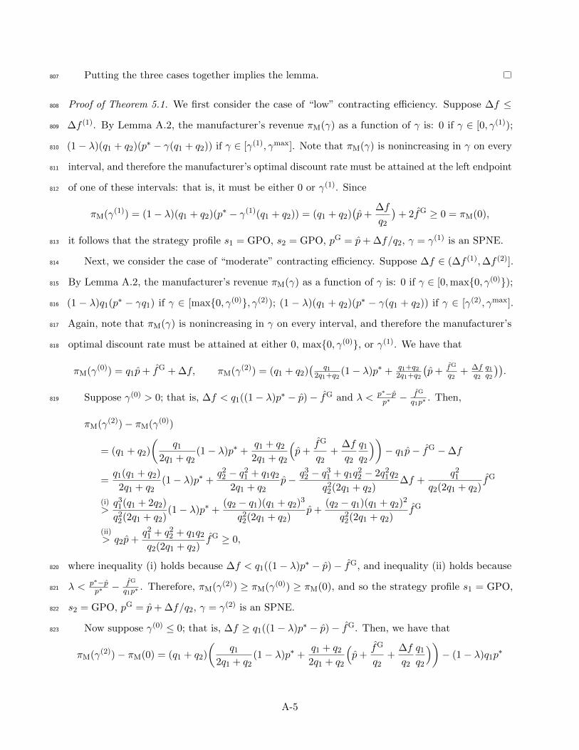
Putting the three cases together implies the lemma.807
Proof of Theorem 5.1. We first consider the case of “low” contracting efficiency. Suppose ∆f ≤808
∆f (1). By Lemma A.2, the manufacturer’s revenue πM(γ) as a function of γ is: 0 if γ ∈ [0, γ(1));809
(1− λ)(q1 + q2)(p∗ − γ(q1 + q2)) if γ ∈ [γ(1), γmax]. Note that πM(γ) is nonincreasing in γ on every810
interval, and therefore the manufacturer’s optimal discount rate must be attained at the left endpoint811
of one of these intervals: that is, it must be either 0 or γ(1). Since812
πM(γ(1)) = (1− λ)(q1 + q2)(p∗ − γ(1)(q1 + q2)) = (q1 + q2)(p̂+
∆f
q2
)+ 2f̂G ≥ 0 = πM(0),
it follows that the strategy profile s1 = GPO, s2 = GPO, pG = p̂+ ∆f/q2, γ = γ(1) is an SPNE.813
Next, we consider the case of “moderate” contracting efficiency. Suppose ∆f ∈ (∆f (1),∆f (2)].814
By Lemma A.2, the manufacturer’s revenue πM(γ) as a function of γ is: 0 if γ ∈ [0,max{0, γ(0)});815
(1 − λ)q1(p∗ − γq1) if γ ∈ [max{0, γ(0)}, γ(2)); (1 − λ)(q1 + q2)(p∗ − γ(q1 + q2)) if γ ∈ [γ(2), γmax].816
Again, note that πM(γ) is nonincreasing in γ on every interval, and therefore the manufacturer’s817
optimal discount rate must be attained at either 0, max{0, γ(0)}, or γ(1). We have that818
πM(γ(0)) = q1p̂+ f̂G + ∆f, πM(γ(2)) = (q1 + q2)( q1
2q1+q2(1− λ)p∗ + q1+q2
2q1+q2
(p̂+ f̂G
q2+ ∆f
q2q1q2
)).
Suppose γ(0) > 0; that is, ∆f < q1((1− λ)p∗ − p̂)− f̂G and λ < p∗−p̂p∗ −
f̂G
q1p∗. Then,819
πM(γ(2))− πM(γ(0))
= (q1 + q2)
(q1
2q1 + q2(1− λ)p∗ +
q1 + q2
2q1 + q2
(p̂+
f̂G
q2+
∆f
q2
q1
q2
))− q1p̂− f̂G −∆f
=q1(q1 + q2)
2q1 + q2(1− λ)p∗ +
q22 − q2
1 + q1q2
2q1 + q2p̂− q3
2 − q31 + q1q
22 − 2q2
1q2
q22(2q1 + q2)
∆f +q2
1
q2(2q1 + q2)f̂G
(i)>q3
1(q1 + 2q2)
q22(2q1 + q2)
(1− λ)p∗ +(q2 − q1)(q1 + q2)3
q22(2q1 + q2)
p̂+(q2 − q1)(q1 + q2)2
q22(2q1 + q2)
f̂G
(ii)> q2p̂+
q21 + q2
2 + q1q2
q2(2q1 + q2)f̂G ≥ 0,
where inequality (i) holds because ∆f < q1((1− λ)p∗ − p̂)− f̂G, and inequality (ii) holds because820
λ < p∗−p̂p∗ −
f̂G
q1p∗. Therefore, πM(γ(2)) ≥ πM(γ(0)) ≥ πM(0), and so the strategy profile s1 = GPO,821
s2 = GPO, pG = p̂+ ∆f/q2, γ = γ(2) is an SPNE.822
Now suppose γ(0) ≤ 0; that is, ∆f ≥ q1((1− λ)p∗ − p̂)− f̂G. Then, we have that823
πM(γ(2))− πM(0) = (q1 + q2)
(q1
2q1 + q2(1− λ)p∗ +
q1 + q2
2q1 + q2
(p̂+
f̂G
q2+
∆f
q2
q1
q2
))− (1− λ)q1p
∗
A-5
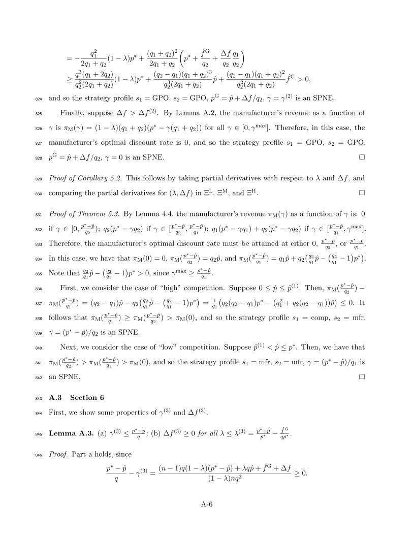
= − q21
2q1 + q2(1− λ)p∗ +
(q1 + q2)2
2q1 + q2
(p∗ +
f̂G
q2+
∆f
q2
q1
q2
)≥ q3
1(q1 + 2q2)
q22(2q1 + q2)
(1− λ)p∗ +(q2 − q1)(q1 + q2)3
q32(2q1 + q2)
p̂+(q2 − q1)(q1 + q2)2
q22(2q1 + q2)
f̂G > 0,
and so the strategy profile s1 = GPO, s2 = GPO, pG = p̂+ ∆f/q2, γ = γ(2) is an SPNE.824
Finally, suppose ∆f > ∆f (2). By Lemma A.2, the manufacturer’s revenue as a function of825
γ is πM(γ) = (1 − λ)(q1 + q2)(p∗ − γ(q1 + q2)) for all γ ∈ [0, γmax]. Therefore, in this case, the826
manufacturer’s optimal discount rate is 0, and so the strategy profile s1 = GPO, s2 = GPO,827
pG = p̂+ ∆f/q2, γ = 0 is an SPNE.828
Proof of Corollary 5.2. This follows by taking partial derivatives with respect to λ and ∆f , and829
comparing the partial derivatives for (λ,∆f) in ΞL, ΞM, and ΞH.830
Proof of Theorem 5.3. By Lemma 4.4, the manufacturer’s revenue πM(γ) as a function of γ is: 0831
if γ ∈ [0, p∗−p̂q2
); q2(p∗ − γq2) if γ ∈ [p∗−p̂q2
, p∗−p̂q1
); q1(p∗ − γq1) + q2(p∗ − γq2) if γ ∈ [p∗−p̂q1
, γmax].832
Therefore, the manufacturer’s optimal discount rate must be attained at either 0, p∗−p̂q2
, or p∗−p̂q1
.833
In this case, we have that πM(0) = 0, πM(p∗−p̂q2
) = q2p̂, and πM(p∗−p̂q1
) = q1p̂+ q2
( q2q1p̂−
( q2q1− 1)p∗).834
Note that q2q1p̂−
( q2q1− 1)p∗ > 0, since γmax ≥ p∗−p̂
q1.835
First, we consider the case of “high” competition. Suppose 0 ≤ p̂ ≤ p̂(1). Then, πM(p∗−p̂q2
) −836
πM(p∗−p̂q1
) = (q2 − q1)p̂ − q2
( q2q1p̂ −
( q2q1− 1)p∗)
= 1q1
(q2(q2 − q1)p∗ − (q2
1 + q2(q2 − q1))p̂)≤ 0. It837
follows that πM(p∗−p̂q1
) ≥ πM(p∗−p̂q2
) > πM(0), and so the strategy profile s1 = comp, s2 = mfr,838
γ = (p∗ − p̂)/q2 is an SPNE.839
Next, we consider the case of “low” competition. Suppose p̂(1) < p̂ ≤ p∗. Then, we have that840
πM(p∗−p̂q2
) > πM(p∗−p̂q1
) > πM(0), and so the strategy profile s1 = mfr, s2 = mfr, γ = (p∗ − p̂)/q1 is841
an SPNE.842
A.3 Section 6843
First, we show some properties of γ(3) and ∆f (3).844
Lemma A.3. (a) γ(3) ≤ p∗−p̂q ; (b) ∆f (3) ≥ 0 for all λ ≤ λ(3) = p∗−p̂
p∗ −f̂G
qp∗ .845
Proof. Part a holds, since846
p∗ − p̂q− γ(3) =
(n− 1)q(1− λ)(p∗ − p̂) + λqp̂+ f̂G + ∆f
(1− λ)nq2≥ 0.
A-6

Part b holds, since ∆f (3) = q(p∗ − p̂)− f̂G − qp∗λ ≥ q(p∗ − p̂)− f̂G − qp∗λ(3) = 0.847
Next, we characterize the optimal strategies of the providers and the GPO as a function of the848
manufacturer’s discount rate γ.849
Lemma A.4. Let γ be any given strategy for the manufacturer.850
a. Given “low” contracting efficiency—i.e., ∆f ≤ ∆f (3)—the optimal strategies of the providers and851
the GPO are: si = comp, pG = +∞ if γ ∈ [0, γ(3)); si = GPO, pG = p̂+ ∆fq if γ ∈ [γ(3), p
∗−p̂q );852
si = GPO, pG = p∗ − γq + ∆fq if γ ∈ [p
∗−p̂q , γmax].853
b. Given “high” contracting efficiency—i.e., ∆f > ∆f (3)—the optimal strategies of the providers854
and the GPO are: si = GPO, pG = p̂ + ∆fq if γ ∈ [0, p
∗−p̂q ); si = GPO, pG = p∗ − γq + ∆f
q if855
γ ∈ [p∗−p̂q , γmax].856
Proof. We consider two cases, based on the level of γ.857
First, suppose γ ∈ [0, p∗−p̂q ), or equivalently, p̂ < p∗ − γq. In this case, by Lemma 4.1, we have858
that: si = GPO if pG ∈ [0, p̂+ ∆fq ]; si = comp if pG ∈ (p̂+ ∆f
q ,+∞). Therefore, the GPO’s optimal859
unit on-contract price pG must be either p̂+ ∆fq or +∞. Note that860
πG(p̂+ ∆fq ) = nf̂G + n∆f − nq((1− λ)p∗ − p̂) + (1− λ)(nq)2γ, πG(+∞) = 0.
If 0 ≤ ∆f < ∆f (3), it is straightforward to show that πG(p̂ + ∆fq ) > πG(+∞) if and only if861
γ > γ(3). Therefore, the GPO’s optimal unit on-contract price pG is: +∞ if γ ∈ [0, γ(3)]; p̂+ ∆fq if862
γ ∈ (γ(3), p∗−p̂q ]. Otherwise, if ∆f ≥ ∆f (3), we have that that πG(p̂+ ∆f
q ) ≥ (1−λ)(nq)2γ ≥ πG(+∞),863
for all γ ∈ [0, p∗−p̂q ). Therefore, in this case, the GPO’s optimal unit on-contract price is pG = p̂+ ∆f
q864
for all γ ∈ [0, p∗−p̂q ).865
Next, suppose γ ∈ [p∗−p̂q , γmax], or equivalently, p∗ − γq ≤ p̂. In this case, by Lemma 4.1, we866
have that: si = GPO if pG ∈ [0, p∗ − γq + ∆fq ]; si = comp if pG ∈ (p∗ − γq + ∆f
q ,+∞). Therefore,867
the GPO’s optimal unit on-contract price pG must be either p∗ − γq + ∆fq or +∞. Note that868
πG(p∗ − γq + ∆fq ) = nf̂G + n∆f + λ(nq)(p∗ − γq) + (1 − λ)n(n − 1)q2γ ≥ 0 = πG(+∞). It869
follows in this case that the GPO’s optimal unit on-contract price is pG = p∗ − γq + ∆fq for all870
γ ∈ [p∗−p̂q , γmax].871
Proof of Theorem 6.1. We first consider the case of “low” contracting efficiency. Suppose 0 ≤ ∆f ≤872
∆f (3). By Lemma A.4, the manufacturer’s revenue πM(γ) as a function of γ is: 0 if γ ∈ [0, γ(3));873
A-7

(1− λ)(nq)(p∗ − γnq) if γ ∈ [γ(3), γmax]. Note that πM(γ) is nonincreasing in γ on every interval,874
and therefore the manufacturer’s optimal discount rate must be attained at the left endpoint of one875
of these intervals: that is, it must be either 0 or γ(3). Since πM(γ(3)) = (1− λ)(nq)(p∗ − γ(3)nq) =876
nq + nf̂G + n∆f > 0 = πM(0), it follows that the strategy profile si = GPO, pG = p̂ + ∆f/q,877
γ = γ(3) is an SPNE.878
Next, we consider part b. By Lemma A.4, the manufacturer’s revenue as a function of γ is879
πM(γ) = (1− λ)nqp∗, and so in this case, the manufacturer’s optimal discount rate is 0. Therefore,880
the strategy profile si = GPO, pG = p̂+ ∆f/q, γ = 0 is an SPNE.881
Proof of Corollary 6.2. This follows by taking partial derivatives with respect to λ and ∆f , and882
comparing the partial derivatives for (λ,∆f) in ΞL and ΞH.883
Proof of Theorem 6.3. By Lemma 4.4, the manufacturer’s revenue πM(γ) as a function of γ is: 0 if884
γ ∈ [0, p∗−p̂q ); (nq)(p∗ − γq) if γ ∈ [p
∗−p̂q , γmax]. Therefore, the manufacturer’s optimal discount rate885
must be attained at either 0 or p∗−p̂q . We have that πM(p
∗−p̂q ) = nqp̂ ≥ 0 = πM(0). Therefore, the886
strategy profile si = mfr, γ = (p∗ − p̂)/q is an SPNE.887
A.4 Section 7888
Proof of Theorem 7.1. Fix some discount schedule p(·). The breakeven price that induces providers889
1, . . . , n to purchase through the GPO is pBn = min{p(qn), p̂}+ ∆f
qn. Similarly, the breakeven price890
that induces providers 1, . . . , k∗ to purchase through the GPO is pBk∗ = min{p(qk∗), p̂} + ∆f
qk∗. It891
follows that892
πG(pBn )− πG(pB
k∗) = (n− k∗)f̂G +n∑i=1
qi
(min{p(qn), p̂} − (1− λ)p
( n∑j=1
qj
))
−k∗∑i=1
qi
(min{p(qk∗), p̂} − (1− λ)p
( k∗∑j=1
qj
))+ ∆f
(1
qn
n−1∑i=1
qi −1
qk∗
k∗−1∑i=1
qi
).
So, if ∆f is sufficiently high, by (7.1), we have that πG(pBn ) < πG(pB
k∗) for any feasible p(·), since893
p(·) is bounded from above and below by a constant that is independent of ∆f . Therefore, if ∆f is894
sufficiently high, regardless of the manufacturer’s choice of discount schedule p(·), the GPO is more895
profitable if it sets its unit price to obtain the business of providers 1, . . . , k∗, instead of all of the896
providers 1, . . . , n.897
A-8


