
Mauro Trapanotto
A.Y. 2014 – 2015
Università degli studi di Padova Dipartimento di Ingegneria Civile, Edile e Ambientale (DICEA)
Laboratoire d’étude des Transferts en Hydrologie et Environnement (LTHE) Équipe: Transferts couples en milieux poreux héterogènes (TRANSPORE)
MASTER THESIS
THE INFLUENCE OF BENTONITE TREATMENT ON SOIL HYDRAULIC PROPERTIES:
APPLICATION TO THE CAP COVER OF A FRENCH DISPOSAL FOR NUCLEAR WASTE OF LOW ACTIVITY
Supervisors:
Prof. Paolo Carrubba Prof. Jean-Pierre Gourc


TABLE OF CONTENTS
ABSTRACT ....................................................................................................................... 9
CHAPTER 1 RADIOACTIVE WASTE MANAGEMENT AND CAP COVER SYSTEM IN NEAR SURFACE DISPOSAL ..................................................................................... 11
1.1 RADIOACTIVE DECAY ................................................................................................ 11
1.2 CLASSIFICATION OF RADIOACTIVE WASTE ................................................................... 14
1.2.1 Classification in France .................................................................................... 18
1.2.2 Classification in Italy ........................................................................................ 19
1.2.3 Classification in the United States .................................................................... 20
1.2.4 Classification in Japan ..................................................................................... 21
1.3 DISPOSAL FACILITIES ................................................................................................ 22
1.3.1 Objectives and safety means of disposal facilities ............................................ 22
1.3.2 Disposal methods ............................................................................................ 23
1.4 CAP COVER SYSTEM IN NEAR SURFACE DISPOSAL ..................................................... 25
1.4.1 Cap cover system functions and composition .................................................. 26
1.4.2 Cap cover system for radioactive waste in France ........................................... 28
1.4.3 Clay layer compaction requirements ................................................................ 29
CHAPTER 2 SATURATED AND UNSATURATED HYDRAULIC CONDUCTIVITY ............................. 33
2.1 SATURATED AND UNSATURATED SOILS ...................................................................... 33
2.1.1 Water content and degree of saturation ........................................................... 35
2.1.2 Pore-water pressure in saturated media .......................................................... 36
2.1.3 Adsorption and capillarity in soils ..................................................................... 37
2.1.4 Suction definition.............................................................................................. 40
2.1.5 Conclusions on pore-water pressure in saturated and unsaturated media ....... 43
2.2 SATURATED HYDRAULIC CONDUCTIVITY ..................................................................... 44

2.2.1 Definition hydraulic conductivity for saturated media ........................................ 44
2.2.2 Permeability and Hydraulic conductivity ........................................................... 46
2.2.3 Methods for measuring KSAT ............................................................................. 47
2.3 UNSATURATED HYDRAULIC CONDUCTIVITY ................................................................. 49
2.3.1 Definition of hydraulic conductivity for unsaturated media ................................ 49
2.3.2 The Soil Water Retention Curve (SWRC)......................................................... 50
2.3.3 The Van Genuchten model .............................................................................. 53
CHAPTER 3 BENTONITE TREATMENTS FOR DISPOSAL PASSIVE BARRIER .............................. 55
3.1 CLAYS COMPOSITION AND PROPERTIES ..................................................................... 55
3.1.1 Bentonite characteristics .................................................................................. 57
3.2 EFFECT OF BENTONITE TREATMENTS ON SOIL PROPERTIES ......................................... 58
3.2.1 Atterberg’s limits .............................................................................................. 58
3.2.2 Methylene blue adsorption test ........................................................................ 60
3.2.3 Compaction properties ..................................................................................... 61
3.2.4 Hydraulic conductivity ...................................................................................... 64
3.3 CONCLUSIONS ON BENTONITE TREATMENTS ............................................................... 68
CHAPTER 4 THE CSM, THE CHARACTERISATION OF THE SOILS OF THE CSM AND THEIR BENTONITE TREATMENTS ....................................................................... 69
4.1 THE CENTRE DE STOCKAGE DE LA MANCHE (CSM) .................................................... 69
4.1.1 History of the CSM ........................................................................................... 70
4.1.2 The cap cover system of the CSM ................................................................... 72
4.1.3 The long term cap cover system ...................................................................... 74
4.2 THE TYPE MATERIALS AND THEIR TREATMENTS ........................................................... 75
4.2.1 Definition of the type materials: T12 and T3 ..................................................... 75
4.2.2 The bentonite treatments ................................................................................. 76
4.3 CLASSIFICATION OF THE SOILS .................................................................................. 76
4.3.1 Granulometric curves ....................................................................................... 77

4.3.2 Methylene blue adsorption test (VBS) .............................................................. 80
4.3.3 Atterberg limits ................................................................................................. 82
4.3.4 Classification of the samples ............................................................................ 86
4.4 SOLID UNIT WEIGHT .................................................................................................. 88
4.5 PROCTOR TEST ........................................................................................................ 89
4.6 SUMMARY OF THE SAMPLES CHARACTERISATION ........................................................ 93
CHAPTER 5 INFLUENCE OF THE TREATMENTS ON HYDRAULIC CONDUCTIVITY IN SATURATED CONDITIONS ....................................................................................... 95
5.1 OEDO-PERMEAMETER TEST ...................................................................................... 95
5.1.1 Samples preparation ........................................................................................ 95
5.1.2 Description of the method ................................................................................ 96
5.1.3 Results ............................................................................................................. 98
5.2 CORRELATIONS BETWEEN KSAT AND SOIL PROPERTIES.............................................. 100
5.2.1 Untreated soils ............................................................................................... 101
5.2.2 Treated soils .................................................................................................. 104
5.3 SUMMARY OF RESULTS ........................................................................................... 107
CHAPTER 6 INFLUENCE OF BENTONITE TREATMENTS ON SOIL IN UNSATURATED CONDITIONS ................................................................................ 109
6.1 DESCRIPTION OF THE HANGING COLUMN TEST .......................................................... 109
6.2 PREPARATION OF THE SAMPLES .............................................................................. 113
6.2.1 Compaction with Proctor procedure ............................................................... 115
6.2.2 Retrieving of the sample with normal compression ........................................ 116
6.2.3 Measure of samples mass, height and volume .............................................. 117
6.3 PRELIMINARIES TO THE TEST ................................................................................... 118
6.3.1 Calculation of samples dry masses and dry unit weights ................................ 119
6.3.2 Calculation of water content parameters ........................................................ 119
6.4 THE TEST PROCESS ................................................................................................ 120

6.4.1 Preparation of the sandbox ............................................................................ 120
6.4.2 Saturation phase ............................................................................................ 122
6.4.3 Suction phase ................................................................................................ 123
6.4.4 Temperature and humidity survey .................................................................. 124
6.4.5 Dry samples masses and filters masses ........................................................ 125
6.5 PROBLEMS ENCOUNTERED AND CORRECTIONS ........................................................ 125
6.5.1 Reference level for the zero suction ............................................................... 126
6.5.2 Overestimation of water content ..................................................................... 126
6.5.3 Assessment of filter mass during the experiment ........................................... 127
6.5.4 Swelling of the samples ................................................................................. 128
6.5.5 Fine material loss from the samples ............................................................... 129
6.5.6 Presence of mushrooms on the sample upper surface .................................. 130
6.5.7 Calculation of the degree of saturation S ....................................................... 130
6.6 APPLICATION OF THE VAN GENUCHTEN MODEL ........................................................ 133
6.6.1 The experimental Soil Water Retention Curve ............................................... 134
6.6.2 The Van Genuchten model parameters ......................................................... 135
6.7 RESULTS ............................................................................................................... 137
6.7.1 Estimation of the solid unit weight .................................................................. 138
6.7.2 Soil Water Retention Curves .......................................................................... 140
6.7.3 Observations on swelling and shrinkage ........................................................ 142
6.7.4 Estimation of the hydraulic conductivity .......................................................... 145
6.8 CONCLUSIONS ON THE HANGING COLUMN TEST ........................................................ 149
CHAPTER 7 SOILS SENSITIVITY TO EROSION .............................................................................. 151
7.1 PRESENTATION OF THE PROBLEM ............................................................................ 151
7.1.1 Possible impact on the behaviour of the landfill soil cover .............................. 153
7.2 INTERNAL AND EXTERNAL EROSION.......................................................................... 154
7.3 INTERNAL STABILIY GEOMETRIC CRITERIA ................................................................. 155

7.3.1 Kezdi’s criterion.............................................................................................. 156
7.3.2 Kenney and Lau’s criterion ............................................................................. 158
7.3.3 Burenkova’s criterion ..................................................................................... 160
7.3.4 Liu’s criterion .................................................................................................. 162
7.3.5 Mao’s criterion ............................................................................................... 163
7.3.6 Conclusions on the internal stability criteria .................................................... 165
7.4 EXTERNAL EROSION CRITERIA ................................................................................. 166
7.4.1 Analysis of the untreated materials ................................................................ 167
7.4.2 Effect of bentonite treatments ........................................................................ 169
7.4.3 Conclusions on the external erosion criteria ................................................... 171
7.5 CONCLUSIONS ON SOILS SENSITIVITY TO EROSION .................................................... 172
CONCLUSIONS ............................................................................................................ 173
ATTACHMENT .............................................................................................................. 175
BIBLIOGRAPHY ........................................................................................................... 189
ACKNOWLEDGEMENTS.............................................................................................. 197


9
ABSTRACT
This work focuses on the influence of bentonite treatment on the properties of two soils
(called T12 and T3) used to realise the clay layer of the cap-cover system of a French
near-surface disposal facility for nuclear waste of low radioactivity: the Centre de Stockage
de la Manche (CSM).
The main aim of the bentonite treatment is to reduce the hydraulic conductivity of the clay
layer in order to provide a long-term impervious barrier.
In chapter 1, the waste management for radioactive waste will be introduced referring in
particular to the documents provided by the International Atomic Energy Agency (IAEA).
After presenting the radioactivity problem in waste facilities, the radioactive waste
classification and the possible disposal methods will be presented. The dissertation will
focus on the characteristics required by the cap-cover system of near-surface disposals.
In chapter 2, the parameters used to define soils in unsaturated and saturated conditions
will be presented: water content measures, capillarity, pore-water pressure and suction. In
particular, the differences between hydraulic conductivity in saturated and unsaturated
conditions will be discussed.
In chapter 3, after defining clay and bentonite properties, the dissertation will focus on the
effect of bentonite treatments on the soil properties. Therefore, some studies about the
bentonite influence on Atterberg limits, VBS value, compaction characteristics and
hydraulic conductivity will be considered.
In chapter 4, the CSM and the soils (T12 and T3) to be analysed and treated will be
presented. The tests, performed to characterise and classify the raw soils and the 5%, 7%,
12% treatments, will be presented.
In chapter 5, the hydraulic conductivity in saturated conditions will be calculated with the
rigid wall oedo-permeameter with variable hydraulic charge and some empirical
correlations. The discussion will focus on the differences between the different approaches
and on the effect of bentonite on the hydraulic conductivity decrease.
In chapter 6, the unsaturated conditions will be considered. In order to build the Soil Water
Retention Curve (SWRC) the hanging column test and the Van Genuchten model will be

10
used. The Van Genuchten model will be applied also to obtain the variation of hydraulic
conductivity with suction and, hence, of the water content.
In chapter 7, the effect of bentonite content on the soil sensitivity to erosion will be
analysed. The urge to analyse this aspect is due to the fine particles loss observed during
the hanging column test. Internal and external erosion criteria will be applied in order to
understand the nature of the phenomenon.

11
CHAPTER 1 Radioactive waste management and Cap Cover System in near surface disposal
In this chapter, the regulations about radioactive waste management will be presented.
After introducing the radioactive decay process (paragraph 1.1), the radioactive waste
classification (paragraph 1.2) and its final disposal (paragraph 1.3) will be described,
referring to the standards provided by the International Atomic Energy Agency (IAEA).
Since the material object of study in the following chapter comes from a French near
surface disposal, in paragraph 1.3 the dissertation will focus on these kind of facilities
referring, in particular, to the characterisation of the cap cover system.
1.1 RADIOACTIVE DECAY
The term radioactive decay (or radioactivity) is used to define all the atomic and nuclear
processes through which an instable atomic nucleus decays into a lower energy nucleus in
order to achieve stability (IAEA, 2009b). This process always takes place with a release of
energy in the form of radiations (atomic particles) implying, sometimes, chemical
transformation and charge loss (Capecchi, 2013).
It is possible to distinguish four groups of radiations (Knoll, 2010):
1. Fast electrons (β rays),
2. Heavy charged particles (α rays, protons, fission products),
3. Electromagnetical radiation (X rays and γ rays),
4. Neutrons.
Each category is characterised by different properties and degree of danger that are
summarised in table 1.1 (Department of the Army, 1993).

12
Name What is it?
Source Energy and
Speed Range in
Air Range in
Tissue Shielding Required
Biological Hazard
α Alpha
particle
Helium Nucleus
Decay of Uranium
and plutonium
Energy varies:
speed varies from 1/20 to 1/10 speed
of light
5 cm Cannot
penetrate the epiderms
None
None unless ingested
or inhaled in sufficient quantities
β Beta
particle
High-speed electron
Decay of fission
products and neutron induced
elements
Varies 5 m Several layers of skin
Stopped by a few cm
or moderate clothing
Superficial skin injury
γ Gamma
ray
Electro-magnetic
energy
Decay of fission
products and neutron induced
elements
Energy varies:
travels at the speed of light
Up to 500 m but energy
dependent
Very penetrating, but energy dependent
Dense material, such as concrete, steel plate,
earth.
Whole body injury, many
casualties possible
Neutron
Uncharged particle
Fission and fusion
reactions Varies
Less than gamma ray but energy dependent
Very penetrating, but energy dependent
Hydrogeous materials,
such as water or damp earth
Whole body injury, many
casualties possible
Table 1.1
In the disposal facilities for radioactive waste is of fundamental interest to prevent the
radiations from spreading in the environment. For this purpose, it is necessary to choose
proper barriers in order to reduce the radiation intensity and stop its transmission. This
operation is commonly called shielding.
In table 1.1 and figure 1.1 (JAEA, 2014), the shielding requirements for each category of
radiation are summarised.
Since β rays and α rays are composed by charged particles, they interact with the
environment and, hence, their energy decreases rapidly in short spaces. They are easily
blocked by thin barriers.
X rays, γ rays and neutrons do not have electric charge and can be absorbed only by
collision between atoms. Therefore, these radiations are able to cover long distances and,
hence, penetrate in the human body. In order to block these emissions, a thicker barrier is
required.

13
Figure 1.1
In order to choose the most appropriate material to realise the barrier, the concept of half-
value layer (HVL) is used. HVL is the thickness of the material at which the radiation
intensity is reduced by one-half (ENS, 2013).
In table 1.2 (De Rose, 2003), some HVL values are displayed for different materials.
Lead, steel, iron and concrete are commonly used as shielding materials. The halving
mass indicates the mass of material necessary to cut radiation by 50%.
Material HVL [cm]
Density [g/cm3]
Halving Mass [g/cm2]
Lead 1 11.3 12
Concrete 6.1 3.33 20
Steel 2.5 7.86 20
Packed soil 9.1 1.99 18
Water 18 1 18
Wood 29 0.56 16
Air 15000 0.0012 18
Table 1.2

14
The radioactivity is a process occurring naturally on earth. Moreover, it can be produced
artificially in many fields such as medicine, food preservation, archaeology, etc. (Capecchi,
2013).
The environment is considered contaminated when a deposition of radioactive substances
is observed on surfaces, solids, liquids or gases (including the human body), in which their
presence is unintended and undesirable (IAEA, 2007).
Considering the waste management context, containment and isolation of radioactive
waste through durable and effective barriers is an important concern not only for countries
involved in the nuclear energy production but also for the rest of the world.
1.2 CLASSIFICATION OF RADIOACTIVE WASTE
The classification of radioactive waste is not homogeneous in the world and it may be
defined at different levels (international level, national level, operator level) according to
the purpose of the classification. Moreover, the development of different schemes
according to physical, chemical and radiological properties has led to different
terminologies, which could cause confusion, especially at the international level, in the
radioactive waste management.
The International Atomic Energy Agency (IAEA) provides the guidelines of the
classification of radioactive waste.
In the General Safety Guide No. GSG-1 a comprehensive range of waste classes has
been defined giving also some general boundary conditions in order to distinguish one
class from the other. The guide underlines that detailed quantitative boundary conditions
must be developed by each country considering a wider range of parameters. Moreover,
the guide underlines that in cases when there is more than a facility in a country, the
quantitative boundaries between the classes may differ for each disposal facility in
accordance with scenarios and geological, technical and safety parameters (IAEA, 2009b).
The classification schemes for radioactive waste may be developed using an approach
related to safety conditions, regulatory aspects or engineering processes necessary for the
waste management.
The different typologies of classification of the radioactive waste are summarized in the
following scheme:

15
Qualitative classification. It is based on the general characteristics of the
radioactive waste. In particular, it is possible to develop different qualitative
classifications according to:
- the origin of the waste;
- the physical state of the waste (solid, liquid, gaseous);
- the activity levels.
Quantitative classification. It provides numerical values to distinguish the waste
classes. The first step to develop this kind of classification is to decide the purpose
of the classification considering the type of waste, the activity under consideration,
the processing options available, the safety objectives, the socio-economic factors
and the regulatory and technical constraints. The second step consists in choosing
the parameters to use for evaluating numerical values as limits for each class of
waste.
The IAEA (2009b) uses essentially two parameters for its classification:
Activity content;
Half-life.
The activity content designates the radioactivity level of the radioactive elements
(radionuclides) contained in the waste (Verstaevel, 2013). The level of radioactivity can be
expressed in Becquerels (Bq) per unit of weight. The Becquerel is the unit of the
radioactive decay; an activity of one Becquerel means that one disintegration occurs
approximately every second (IAEA, 2009b).
The half-life of a radioactive isotope is the time taken for it to decay to half of its amount of
radioactivity as measured at the beginning of the time period considered. It can be
expressed in years, minutes or seconds.
In the graphic of figure 1.2 (Verstaevel, 2013), it is possible to see the evolution of the
activity content with time. The relation between the two parameters is exponential. The
half-life corresponds to the value of time at which the activity level is equal to A0/2 where
A0 is the initial activity content.

16
Figure 1.2
The IAEA (2009b) distinguishes 6 classes of waste:
Exempt waste (EW);
Very short lived waste (VSLW);
Very low level waste (VLLW);
Low level waste (LLW)
Intermediate level waste (ILW)
High level waste (HLW)
The exempt waste (EW) is characterized by a concentration of radionuclides, which is so
small that it does not require any specific provision for the control and the radiations.
Hence, this kind of material can be disposed in conventional landfills or recycled.
The very short-lived waste (VSLW) contains radionuclides characterized by a very short
half-life but with an activity concentration above the authorized level. In general, this kind
of waste undergoes storage for decay until the activity is minor of the authorized level.
After the VSLW re-enters into the clearance zone, it moves to the class of the EW and
hence it can be managed as a conventional waste.
The very low-level waste (VLLW) is characterized by a level of activity that still does not
require high levels of isolation and containment. This type of waste can be disposed in
surface landfill facilities with limited regulatory controls.
The low-level waste (LLW) is above the clearance level but it contains only limited
amounts of long-lived radionuclides. In general, this kind of waste can include short-lived
radionuclides at high level of activity concentration and long lived radionuclides but only at

17
low level of activity. The LLW needs to be stocked into facilities, which provide isolation
and containment for limited periods. This type of waste is still suitable for near surface
disposal but there are different design options for the realization of the facility since the
LLW could be characterized by a wide range of activity levels.
The intermediate level waste (ILW) is characterized by the presence of long-lived
radionuclides in quantities, which require a greater level of isolation and containment from
the environment. In this case, the disposal in the surface facility is not adequate to reach
the needed containment. Therefore, the disposal of the ILW has to be done into facilities at
a depth generally between a few tens and a few hundreds of metres. Nevertheless, this
kind of waste generally does not need particular provision to prevent heat dissipation
during the operations of storage and disposal.
The high-level waste (HLW) is characterized by high levels of activity concentration. In this
kind of waste, the radioactive decay process generate quantities of heat, which have to be
considered in the design of the facility. The disposal of the HLW has to be done into stable
geological formations at a depth of several hundred metres below the surface.
In figure 1.3, the concept of the IAEA classification is displayed. Considering the vertical
axis, it is possible to notice that the higher the level of activity content the greater the
urgency to provide to an adequate isolation from the biosphere. Considering the horizontal
axis, it is possible to assert that, over a certain value of activity content, the higher the half-
life the greater the need to isolate the waste.
Figure 1.3

18
1.2.1 Classification in France
In France, the management of radioactive wastes are regulated by the Andra (Agence
nationale pour la gestion des déchets radioactifs). The classification is based on the same
parameters used by the IAEA: the activity content and the half-life.
Concerning the activity content, it is possible to distinguish four classes of waste:
Very low level (VLL) – from 1 to 100 Bq/g;
Low level (LL) – from 100 to 100 000 Bq/g;
Intermediate level (IL) – from 100 000 to 1 000 000 Bq/g;
High level (HL) – more than 1 000 000 Bq/g
Concerning the half-life, it is possible to identify three different classes of waste:
Very short lifetime (VSL) – half-life < 100 days;
Short lifetime (SL) – half-life ≤ 31 years;
Long lifetime (LL) – half-life ≥ 31 years.
In figure 1.4, the French classification is summarized.
Figure 1.4

19
1.2.2 Classification in Italy
In Italy, the organism of reference for the management of radioactive waste is the Ispra
(Istituto superiore per la protezione e la ricerca ambientale). The classification is regulated
by the Technical Guide n°26 by ENEA-DISP (now ISPRA) published in 1987. Even though
this norm is not up to date, it is still the norm of reference for the classification of the
radioactive wastes. The radioactive waste is classified into three categories:
Category I: waste characterized by radioactivity decay of months or few years
(mainly hospital and research waste).
The disposal occurs according to general waste regulations.
Category II: waste characterized by decay to radioactivity level of few hundreds
Bq/g in few centuries and by a content of long-life radionuclides with an activity
level minor than 3700 Bq/g in the already conditioned waste.
The disposal occurs near the surface. In particular, the normative provides specific
values of acceptance for shallow land disposal.
Category III: waste characterized by decay to few hundreds of Bq/g in few
thousands of years and by a content of long-life radionuclides with an activity level
superior to 3700 Bq/g in the already conditioned waste.
The disposal occurs in deep geological formations.
In figure 1.5, the Italian approach to the radioactive waste classification is summarized.
Figure 1.5

20
1.2.3 Classification in the United States
In the United States the management of radioactive wastes is mostly regulated by the
NRC (Nuclear Regulatory Commission), in particular for what concerns the LLW, HLW, the
use of uranium and thorium, special nuclear material and by-product material (material that
becomes radioactive into a reactor) (Tonkay, 2005).
The DOE (Department of Energy) manages and regulates specific activities within the
federal government for energy research and national defence purposes. These activities
are subjected to different regulations than the ones managed by the NRC (Tonkay, 2005).
Therefore the classification of radioactive waste is distinguished into two branches (figure
1.6, Tonkay, 2005) depending if the waste belongs to a commercial entity (NRC) or to a
governmental entity (DOE). In the first case the reference is the NRC regulation while in
the second case it is DOE regulation and in particular the Order 435.1, Radioactive Waste
Management.
Figure 1.6

21
The categories of the classification are the following:
High level waste (HLW)
Low-level waste (LLW). According to the NRC classification (NRC,2014), the LLW
are further classified in the following classes based on hazard, disposal and waste
form principles:
Class A – wastes of this class are segregated from the other wastes in the
disposal site; they have to satisfy the minimum requirements defined by the
(NRC, 2014, Title 10, §61.56a).
Class B – wastes of this class must meet both the minimum requirements
(NRC, 2014, Title 10, §61.56a) and the stability requirements (NRC, Title 10,
§61.56b).
Class C – wastes of this class must meet both the minimum requirements
(NRC, Title 10, §61.56a) and the stability requirements (NRC, 2014, Title 10,
§61.56b) and need special measures at the disposal site to prevent inadvertent
intrusion.
Greater than class C (GTCC) – wastes of this class in general are not
acceptable for the near-surface disposal; therefore, it is necessary to take
specific measures for their disposal. In absence of specific measures, these
wastes are disposed into geological formations.
Transuranic waste (TRU Waste)
By-product
1.2.4 Classification in Japan
In Japan, the classification of radioactive waste is provided by the JAEA (Japan Atomic
Energy Agency). The radioactive waste is classified in two main categories according to
the activity level (JAEA, 2014):
High-level waste (HLW) – wastes that after the recovery of uranium and plutonium
in Reprocessing facilities still have high activity contents; these wastes are
disposed in deep geological formations. NUMO (Nuclear waste management
organization of Japan) is the responsible for the geological disposal of HLW.
Low level waste (LLW) – this category includes the following subcategories:

22
Waste from power reactors:
- Relatively higher radioactive waste (under surface disposal);
- Relatively lower radioactive waste, (near surface disposal, generally
concrete pit type);
- Very low level radioactive waste, (near surface disposal, generally
trench type).
Waste containing transuranic nuclides (TRU Waste) (geological disposal,
sub-surface disposal, surface disposal or near surface disposal);
Uranium Waste (geological disposal, sub-surface disposal or near surface
disposal).
Waste under the clearance level is reused or disposed as general wastes.
1.3 DISPOSAL FACILITIES
As the classification of the radioactive waste, the disposal methods may change from
country to country but the IAEA provides the general guidelines in its guides.
As stated by the IAEA, “the disposal of radioactive waste represents the final step in its
management, and disposal facilities are designed, operated and closed with a view to
providing the necessary degree of containment and isolation to ensure safety. The
fundamental safety objective is to protect people and the environment from harmful effects
of ionizing radiation” (IAEA, 2012).
The word “disposal” is used to refer to “the emplacement of radioactive waste into a facility
or a location with no intention of retrieving the waste” (IAEA, 2012) while the word
“storage” is used to refer to “the retention of radioactive waste in a facility or a location with
the intention of retrieving the waste” (IAEA, 2012). Both the typologies of facilities have to
be designed to isolate the waste from the biosphere and hence to ensure an appropriate
level of safety.
1.3.1 Objectives and safety means of disposal facilities
The main objective of disposal is to provide containment and isolation of the waste.
The aim of containment is to protect the environment from the waste until radioactive
decay has reduced significantly the hazard of the waste.

23
The aim of isolation is to retain the waste and to keep its hazard away from the accessible
biosphere and from people through physical separation, which restricts the mobility of
long-lived radionuclides makes human access difficult.
The means to reach adequate levels of containment and isolation of the radioactive waste
depend on the hazard of the waste and, hence, on the typology of disposal chosen.
Containment and isolation can be provided by active or passive means.
Active means consist essentially in the monitoring and the surveillance of the disposal
facility in order to prevent unauthorised or involuntary access to the waste and in general
all disturbance of the facility (IAEA, 2014).
Passive means mainly consist in durable physical barriers which contain and isolate the
waste from the biosphere and make inadvertent intrusion more difficult (IAEA, 2014). The
design of the barrier differs according to the typology of the disposal (geological or near
surface), the waste characteristics and the Country regulations.
In general, the safety of the facility must be mainly provided by passive means in order to
minimise the measures that have to be taken after the closure of the facility (IAEA, 2011).
1.3.2 Disposal methods
It is possible to distinguish the disposal in two main typologies:
Deep geological disposal
Near surface disposal
The geological disposal is used the radioactive waste representing a significant hazard for
the biosphere for long time periods and, hence, not suitable for a disposal in a
conventional landfill or in a near surface facility. Therefore, the geological disposal has
been recommended as a long-term management solution for intermediate level (ILW) and
high level (HLW) radioactive waste (IAEA, 2011).
The geological disposal consists in disposing the solid radioactive waste in an
underground facility positioned in a stable geological formation in order to contain and
isolate the waste from the biosphere for long periods.
The containment can be provided by durable packaging of waste, engineered barriers and
host geological formation.
The isolation is provided by the host geological formation itself.
The overall performance of the facility relies essentially on the properties such as retention

24
capability, low permeability and homogeneity of the geological formation, which must delay
the contact of the radioactive waste with the biosphere until its impact is not more
hazardous than the naturally occurring radioactivity (Andra, 2011).
The geological disposal is a method still under study nowadays. Therefore, the knowledge
on the phases for the development of this kind of facility, in particular the closure phase, is
still limited.
A scheme of a deep geological disposal is displayed in figure 1.7 (VAE, 2008).
Figure 1.7
The near surface disposal consists in the emplacement of solid radioactive waste in
earthen trenches or in ground-engineered structures above or just below the ground
surface, with a maximum depth up to a few tens of metres. This typology of disposal is
suitable for the disposal of VLLW and LLW (IAEA, 2014).
In order to guarantee a high level of safety, the main concern is to provide containment
and isolation of the facility through appropriate engineered barriers.
The engineered barriers include the design of waste form and packaging, the barriers used
during the operative period and, when the facility is closed, and the cap-cover system for
the long-term protection.
The engineered barriers provide containment of the radionuclides associated with the

25
waste until radioactive decay has significantly reduced the hazard posed by waste (IAEA,
2014).
The engineered barriers can be based on the chemical barrier or the physical barrier
concept.
The chemical containment relates primarily to the retardation of the migration of
radionuclides by reduction of their solubility and by sorption of radionuclides onto a
substrate material. Hence, it consists generally in the use of cementitious waste forms.
The physical containment relates to the prevention of radionuclide migration by means of
barriers characterised by a low permeability.
In most environments, prevention and limitation of ingress of water, coupled with chemical
containment, are key determinants of the safety of near surface disposal.
A scheme of a near surface disposal is displayed in figure 1.8 (VAE, 2008).
Figure 1.8
1.4 CAP COVER SYSTEM IN NEAR SURFACE DISPOSAL
The soils object of study come from the cap cover system of the Centre de Stockage de La
Manche (CSM), a near surface disposal facility. The CSM will be described in detail in
chapter 4, while, in this paragraph, the attention will be focused on the general dispositions
adopted for near surface disposal systems, referring, in particular, to the cap cover system
requirements.
The dissertation will follow the IAEA guidelines for the general matters and the French
guidelines for the cap cover system characterisation.

26
1.4.1 Cap cover system functions and composition
The cap cover system of the near surface disposal consists in a multi-layer barrier, in
which each layer has specific functions and characteristics. It is placed on the near surface
disposal when its exploitation is finished.
The conception of the cap cover system varies in function of the legislation of the country
in which the near surface disposal is. However, some aspects have general value
regardless of the particular situation of the disposal.
According to IAEA (2004), the cap cover system of a facility has the following functions:
Avoid the penetration of water in the facility,
Avoid intrusions perpetrated by plants, animals and humans,
Avoid the dispersion of radon,
Limit the radiations,
Avoid the superficial erosion.
The factors to take into account for the cap cover design are the following:
Nature of the waste,
Cover geometry (layers thickness and slope),
Configuration of the site,
Materials availability,
Climatic conditions (rain, erosion, freeze-thaw cycle, etc.),
Future of the site.
In figure 1.9 (IAEA, 2003), a schematic disposition of the cap cover system in the near
surface disposal is displayed.

27
Figure 1.9
In order to satisfy the objectives and the constraints, the cap cover system consists
generally in five different layers, which are from the bottom to the top:
Support layer above the waste in order to provide a regular base for the other
layers,
Low permeability layer in order to avoid water infiltrations in the waste and leaks
from the waste,
Drainage layer, which collects water not drained away through runoff,
Protective layer against human, animal and plant intrusions and against climatic
cycles (freeze-thaw and wetting-drying),
Superficial layer, which integrates the site in the environment and protects the
cover system from erosion and the climatic agents.
In figure 1.10 (Van Impe, 1998), different configurations of the cap cover system used in
different countries and for different waste typologies are displayed.
Generally, the impermeable function is performed by a low permeability clay layer, often
associated to geosynthetics with barrier function (geomembranes).

28
Figure 1.10
1.4.2 Cap cover system for radioactive waste in France
According to the French norm, the design of the cap cover system for radioactive waste
disposal has to satisfy the prescriptions of the decree of 30rd December 2002, regarding
the disposal for dangerous waste. In particular, article 25 gives the geometric and
hydraulic characteristics required by the cap cover.
According to this article, the cap cover system must be composed by the following layers,
from the bottom to the top:
Draining layer above the waste,
Layer of 1 m characterised by low hydraulic conductivity (K<10-9m/s),
Impermeable barrier realised with a geosynthetic, usually a geomembrane,
Draining layer of 0,50 m (K>10-4m/s),
Vegetative cover of 0,30 m.

29
In figure 1.11, the cap cover system prescribed by the decree is displayed.
Figure 1.11
1.4.3 Clay layer compaction requirements
As seen in figure 1.10, in the near surface disposal for dangerous waste of Europe and
USA, the impermeable and protective function is always entrusted to a low permeability
clay layer. Hence, in this paragraph, the clay layer requirements will be exposed.
The clay layer has to be characterised by a low hydraulic conductivity (K<10-9 m/s), by
good mechanical resistance (high shear strength) and a low shrinkage limit.
Given the soil, these characteristics depend on the compaction conditions in situ and,
hence, on the water content and on the energy of compaction.
The Technical Committee 5 of the International Society for Soil Mechanics and Foundation
Engineering (ISSMFE) has proposed the ideal compaction characteristics for the clay layer
installation.
Considering a fixed energy of compaction, the graphic in figure 1.12 (Camp, 2009) shows
the areas corresponding to good resistance and hydraulic conductivity values for a cap
cover system in function of the water content used in the installation.

30
Figure 1.12
Limit 1 corresponds to the optimum water content line and represents the inferior limit of
the acceptable zone in terms of low hydraulic conductivity.
Limit 2 corresponds to the maximum water content allowed not to have cracking due to
shrinkage. This limit was determined by Daniel and Wu (1993) studying the evolution of
volume deformation in function of the soil water content.
Limit 3 and limit 4 are respectively the maximum water content and the minimum dry unit
weight, at which the soil has a compression resistance of 200 kPa at least (Daniel and Wu,
1993). Hence, the shear resistance increases with the increase of the dry unit weight and
the decrease of the water content.
The intersection of the defined zones correspond to the compaction conditions and, hence,
the couples (w, γd), for which hydraulic conductivity, shrinkage resistance and shear
resistance are characterised by acceptable values.
Referring to the French guidelines, the Bureau de Recherches Géologiques et Minières
(BRGM) has defined the compaction domain in order to have a clay layer with acceptable
hydraulic and mechanical characteristics. The domain is shown in figure 1.13 (BRGM,
2001).

31
Figure 1.13
According to BRGM, the water content to use for the installation and the compaction of a
clay layer for a cap cover system must be comprised between wOPT+2% and wOPT+6%.
This indication will be used for the compactions with the standard Proctor procedure
performed to prepare the soil samples to be tested with the oedo-permeameter (chapter 5)
and the hanging column test (chapter 6).

32

33
CHAPTER 2 Saturated and unsaturated hydraulic conductivity
In this chapter, the soil behaviour in saturated and unsaturated conditions will be
described.
In paragraph 2.1, the parameters necessary to define saturated and unsaturated soils will
be introduced.
In paragraph 2.2 and 2.3, the hydraulic conductivity in saturated and unsaturated
conditions, respectively, will be defined.
2.1 SATURATED AND UNSATURATED SOILS
A soil is saturated when all its porosities are filled by water. Hence, a saturated soil can be
considered a biphasic material composed by a solid phase (soil particles) and a liquid
phase (water filling the pores).
A soil is unsaturated when its porosities are not completely filled by water. Hence, an
unsaturated soil can be considered a multiphasic material composed by a solid phase (soil
particles), a liquid phase (water partially filling the pores) and a gaseous phase (air filling
the rest of the pores).
Unsaturated soils form the largest category of soils present in nature and do not adhere in
behaviour to the classical saturated soil mechanics (Fredlund et al., 2011).
Due to its multiphasic nature, the analysis of unsaturated soils behaviour is more
complicated than saturated soils ones. The physical behaviour of unsaturated soil is
usually formulated with differential equations that must be solved with a numerical
approach. These approaches and the models used to describe the material behaviour play
an important role in solving problems related to unsaturated soils (Fredlund et al. 2011).

34
Figure 2.1
The ground surface climate is an important factor that controls the depth of the
groundwater table and, hence, the thickness of the unsaturated zone. In figure 2.2, a
schematic representation of the subdivision between the saturated and unsaturated zone
in the environment is represented (Fredlund et al., 2011).
Figure 2.2

35
Since the unsaturated zone includes also almost saturated soil (the capillary zone
immediately above the water table), the correct word to label it is “vadose zone” (vadose is
the Latin word for shallow). However, in geotechnical engineering, the term unsaturated
zone has become more common to refer to the part of the ground soil subjected to
negative pore-water pressures (Fredlund et al., 2011).
In order to describe and to study unsaturated soils, it is necessary to define the soil water
content and the pore-water pressure.
In the following paragraphs, the parameters used to define the water content and the pore-
water pressure in saturated media and unsaturated media will be defined.
2.1.1 Water content and degree of saturation
The soil water content is the quantity of water contained in the soil porosities. It is
expressed as a ratio in massic (gravimetric) or volumetric basis.
The following equation defines the gravimetric water content:
𝑤 =𝑚𝑤
𝑚𝑑=
𝑚ℎ − 𝑚𝑑
𝑚𝑑 (2.1)
Where mw (g) is the water mass in the sample calculated as the difference between the
soil sample mass mh (g) and the dry sample mass md (g).
On the other hand, the volumetric water content is defined by the following equation:
𝜃 =𝑉𝑤
𝑉𝑡𝑜𝑡=
𝑉𝑤
𝑉𝑠 + 𝑉𝑣 (2.2)
Where Vw (cm3) is the water volume in the sample and Vtot (cm3) is the total volume of the
sample, which consists in the sum of the solid soil particles volume Vs (cm3) and the voids
volume Vv (cm3) filled by water and/or air.
Volumetric water content can be expressed in function of the gravimetric water content
with the following expression:
𝜃 = 𝑤 ∙𝛾𝑑
𝛾𝑤 (2.3)
Where γd is the dry soil unit weight (kN/m3) and γw is the water unit weight (kN/m3).
The effective saturation degree of a soil, also called normalised water content, is a
dimensionless value defined by Van Genuchten (1980) with the following equation:
36
𝑆 =𝜃 − 𝜃𝑟
𝜃𝑠𝑎𝑡 − 𝜃𝑟 (2.4)
Where θ is the volumetric water content of the sample, θr is the residual volumetric content
of the sample and θsat is the saturated volumetric water content, which, hence, is equal to
the soil porosity n.
The value of S ranges from 0 % (dry conditions) to 100 % (saturated conditions).
The residual volumetric water content can be measured experimentally by determining the
water content on very dry soil. Nevertheless, since this measurement is not made
routinely, θr value can be extrapolated from soil retention data as the lowest water content
value at which the gradient dθ/ds (where s is the suction) becomes zero. However, the
rigorous calculation of θr is unimportant for most practical field problems (Van Genuchten,
1980).
2.1.2 Pore-water pressure in saturated media
Since soil is a multiphasic material, it is necessary to define a relationship, which describes
the interaction between the soil particles and the water filling the voids.
Considering a saturated soil element subjected to forces, Terzaghi distinguishes two kinds
of pressures: the effective stresses and the pore-water stresses.
Effective stresses are transmitted through contact between the soil particles. A soil
compression behaviour and shear strength depend on them.
Pore-water stresses are transmitted through water filling the voids and are also called
neutral stresses (Colombo, 2004).
Effective stresses can be calculated as a difference between the total stress, which
depends on the total weight (soil + water), and the neutral pressure (Terzaghi, 1948).
Hence, it is possible to define effective stress principle with the following equation:
𝜎′ = 𝜎 − 𝑢 (2.5)
Where σ’ is the effective stress (Pa), σ is the total stress (Pa) and u is the neutral stress
(Pa).
Thanks to equation 2.5, it is possible to consider separately the solid phase (soil particles)
and the liquid phase (water filling the voids) of a saturated medium.
Therefore, despite the presence of the soil particles, the pore-water pressure can be
calculated with the classic hydraulic relation regardless of the solid phase.

37
In order to calculate the hydraulic head, the Bernoulli’s equation for incompressible fluids
and steady state flow can be used. Neglecting the inertial head and the transformation of
mechanical energy into thermal energy, the Bernoulli’s principle can be expressed in the
following form (Vicaire, 2006)
ℎ = 𝑧 +𝑢𝑤
𝛾𝑤+
𝑣2
2𝑔 (2.6)
Where h is the hydraulic head of the point P in respect of a horizontal arbitrary datum (m),
z is the elevation of point P in respect of the reference plan (m), uw is the pore-water
pressure in the point P (Pa), γw is water unit weight (kN/m3) and v is the groundwater
velocity in the point P (m/s).
The sum of the first and the second term of equation 2.6 corresponds to the piezometric
head.
The third term is the kinetic head and can be neglected because of the small values of
velocities in porous media.
Setting z=0, equation 2.6 can be simplified:
ℎ =𝑢𝑤
𝛾𝑤 (2.7)
Hence, it is finally possible to calculate the pore-water pressure from equation 2.7:
𝑢 = 𝛾𝑤 ∙ ℎ (2.8)
In hydrostatic conditions, the pore-water pressure increases linearly from the surface table
(z=0) to the bottom of the aquifer (z=H). Hence, in saturated media, the pore-water
pressure is always a positive value.
After having determined the water table position in the soil, the calculation of the pore-
water pressure distribution under the water table can be easily determined.
2.1.3 Adsorption and capillarity in soils
In unsaturated soils, water is not submitted only to gravitational force but also to
adsorption and capillarity forces. In the porous media, these forces cannot be separated
and their joint effect is known as the soil-water interaction (Vicaire, 2006).
Adsorption is due to electrostatic forces, which depend on the chemical structure of the
soil particles and, the soil voids dimensions and the water content. These forces are able

38
to retain water molecules and cations in the capillarity between the soil particles.
These retaining forces decrease with the increase of the water content. When soil is less
humid, its avidity for water is greater and water is strongly retained into the voids. When
the soil is more humid, the retaining forces decreases and water is less retained. In
saturation conditions, these forces are equal to zero.
Water adsorption forces are particularly strong in clays because of their huge specific
surfaces, while for granular soils are less relevant.
Capillarity is the ability of a liquid to flow in narrow spaces in opposition to gravity. In order
to understand this phenomenon, it is useful to analyse the capillary rise of water in a glass
tube with a small diameter, as shown in figure 2.3 (Facciorusso et al., 2011).
Figure 2.3
It is possible to notice that the separation surface between water and air (meniscus) is
concave. The separation surface behaves as an elastic membrane in equilibrium
subjected to water and air pressures. The meniscus is concave because the atmospheric
pressure is higher than the water pressure (Facciorusso, 2011).
Therefore, considering figure 2.3, point 1 and point 2 are characterised by atmospheric
pressure, conventionally set as a reference and, hence, equal to zero.
In the glass tube, water pressure decreases linearly under the atmospheric pressure. The
minimum value is reached at point 3 and can be calculated with the following expression:
𝑢𝑤 = −𝛾𝑤ℎ𝑐 (2.9)

39
Where uw is the water pressure (Pa) and hc is the water rise height (m).
Referring to the situation displayed in figure 2.3, hc is calculated with the following
expression:
ℎ𝑐 =2 𝑇
𝑟 𝛾𝑤cos 𝛼 (2.10)
Where T is the superficial tension on the membrane (Pa), r is the glass tube radius (m),
α is the contact angle of the meniscus with the tube (rad).
In table 2.1 (modified from Weast et al., 1982), the variation of water density ρw and
superficial tension T with the temperature is displayed.
Temperature [°C] ρw [g/cm3] T [N/m]
0 0,9998 0,0756
10 0,9997 0,0742
20 0,9982 0,0728
25 0,9970 0,0720
40 0,9922 0,0696
Table 2.1
Considering a contact angle equal to zero (α=0°) and a water temperature of 20°C, the
variation of the water rise height hc with the glass tube radius r is displayed in figure 2.4.
Figure 2.4

40
Figure 2.5
Considering a column of soil, (figure 2.5) the water rises from the water table through the
canals formed by the soil voids. The water rise height depends on several factors
(Facciorusso, 2011):
Tortuosity of the canals,
Rugosity of the canals,
Dimensions of the voids,
Soil nature.
The irregularities existing in the pores distribution and in the particles structure do not
allow to develop a theory based only on capillarity or on microscopical properties.
For this reason, a macroscopic point of view is needed and the definition of suction is
introduced.
2.1.4 Suction definition
Suction definition is closely related to the pore structure of the material. In fact, the pore
structure determines how the soil works for the transport of water through the connected
pore spaces (Dexter et al, 2007).
The soil porosity distribution depends on the hierarchy of the particles in the soil structure.
In general, it is possible to distinguish the following groups of soil particles, listed in
hierarchical order (Dexter et al., 2007):
1. Primary particles,

41
2. Micro-aggregates,
3. Aggregates,
4. Clods or bulk soil.
The mean size of the pores separating the compound particles of progressively higher
levels are themselves progressively bigger. The total porosity consists in the following
contributes (Dexter et al., 2007):
1. Residual porosity.
It corresponds to the smallest voids of the pore distribution. They are filled by the
residual water (paragraph 2.1.1).
2. Matrix porosity.
It corresponds to the pore space between individual soil mineral particles.
3. Structural porosity.
It corresponds to the pore space between the micro aggregates too. In general,
these pores are mainly composed of micro-cracks, which have an important role in
transport processes.
4. Macro porosity.
It corresponds to the largest porosities in the soil structure.
Since residual porosity and macro porosity are respectively too small and too large to be
characterised in standard water retention experiments, they are not considered for suction
definition.
Total suction Ψ characterises the unsaturated soil tendency to attire water (Facciorusso,
2011). It is defined with the following equation:
𝛹 = 𝑠 + 𝜋 (2.11)
Where s is the matric suction (Pa) and π is the osmotic suction (Pa).
Matric suction s is defined as the difference between the air pressure (ua) and the water
pressure (uw) into porosities of an unsaturated soil:
𝑠 = 𝑢𝑎 − 𝑢𝑤 (2.12)
Where uw is always lower than ua due to the capillarity effect (paragraph 2.1.3)
In natural conditions, ua is equal to the atmospheric pressure and, hence, can be set as
the reference and neglected.

42
Osmotic suction π is due to the presence of dissolved cations in the interstitial water and,
hence, to the electro-chemical potential difference between interstitial and free water
(adsorption effect, paragraph 2.1.3). Osmotic suction is variable with dissolved cations
content of water and is present in saturated soils too.
In geotechnical engineering, osmotic suction is generally neglected and the problems of
the unsaturated soils are referred to matric suction variations. This approximation can be
justified observing the graphic in figure 2.6 (Fredlund et al., 2011).
Figure 2.6
In figure 2.6, total suction, matric suction and osmotic suction variations in function of the
gravimetric water content of a clay are displayed. It is possible to notice that the osmotic
suction remains almost constant with the water content variation. Therefore, fixed a water
content variation Δw, total suction variation ΔΨ is equal to matric suction variation Δs.
In order to measure in situ suction, tensiometers can be used.
A tensiometer consists in a tube with a ceramic porous tip and a water reservoir at the
other extremity. After inserting the instrument into the soil, water flows through the ceramic
43
tip, determining a depression in the reservoir. The depression, corresponding to the
suction value, can be measured with a manometer (Facciorusso, 2011).
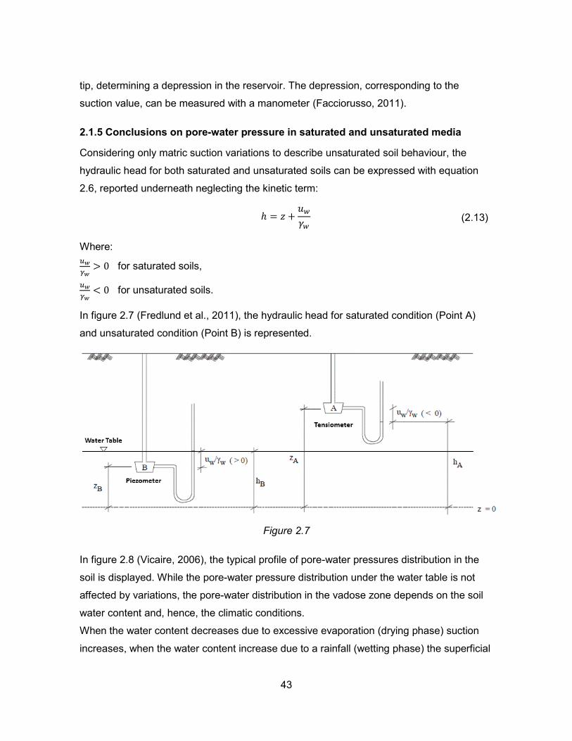
2.1.5 Conclusions on pore-water pressure in saturated and unsaturated media
Considering only matric suction variations to describe unsaturated soil behaviour, the
hydraulic head for both saturated and unsaturated soils can be expressed with equation
2.6, reported underneath neglecting the kinetic term:
ℎ = 𝑧 +𝑢𝑤
𝛾𝑤 (2.13)
Where: 𝑢𝑤
𝛾𝑤> 0 for saturated soils,
𝑢𝑤
𝛾𝑤< 0 for unsaturated soils.
In figure 2.7 (Fredlund et al., 2011), the hydraulic head for saturated condition (Point A)
and unsaturated condition (Point B) is represented.
Figure 2.7
In figure 2.8 (Vicaire, 2006), the typical profile of pore-water pressures distribution in the
soil is displayed. While the pore-water pressure distribution under the water table is not
affected by variations, the pore-water distribution in the vadose zone depends on the soil
water content and, hence, the climatic conditions.
When the water content decreases due to excessive evaporation (drying phase) suction
increases, when the water content increase due to a rainfall (wetting phase) the superficial

44
soil tends to saturated conditions and, as a consequence, suction decreases.
Theoretically, considering moisture equilibrium and no water movement in the vadose
zone, suction is in equilibrium with the water table. This situation could be schematised
with an imaginary infinite impervious membrane on the ground surface (Vicaire, 2006).
Figure 2.8
2.2 SATURATED HYDRAULIC CONDUCTIVITY
In this paragraph, the hydraulic conductivity for saturated media (Ksat) will be introduced.
In particular, Ksat will be defined from the Darcy’s law (paragraph 2.2.1) stressing the
conceptual difference with the medium permeability (paragraph 2.2.2) and introducing
some methods for its measure (paragraph 2.2.3).
2.2.1 Definition hydraulic conductivity for saturated media
Studying the water laminar flow through horizontal sand layers, Darcy found that apparent
velocity through porous media is directly proportional to the hydraulic loss and inversely
proportional to the path followed by water. Later he verified that this relation is also valid

45
for clays and, in general, for all soils (Colombo, 2004).
These concepts are summarised by Darcy’s law:
𝑣 = 𝐾𝑠𝑎𝑡 ∙ 𝑖 (2.14)
Where v is the flow velocity (m/s), Ksat is the hydraulic conductivity of the saturated porous
medium (m/s) and i is the hydraulic gradient (adimensional) which corresponds to the
piezometric line slope.
The hydraulic gradient is calculated with the following equation:
𝑖 =∆𝐻
𝐿 (2.15)
Where ΔH is the hydraulic loss (m) and L is the shortest path followed by water (m).
Ksat is influenced by several factors (Colombo, 2004):
Soil particles dimensions and granulometric distribution,
Soil particles nature and mineralogy,
Particles disposition into the soil,
Material density and compaction properties.
Moreover, the in situ effects like soil stratification and organic deposits should be
considered too.
In table 2.2, values of Ksat according to the soil typology are displayed (Colombo, 2004).
Ksat (m/s) 1 10-1 10-2 10-3 10-4 10-5 10-6 10-7 10-8 10-9 10-10
Pervious Semi-pervious Impervious
Gravel Clean sand and gravel
mixed with clean sand
Fine sand, organic and
inorganic silt, sand
mixed with silt or clay,
clay deposits
Homogeneous
clays
Table 2.2
Ksat is characterised by a huge range of variability and becomes higher with the increase of
soil particles dimensions.

46
2.2.2 Permeability and Hydraulic conductivity
Even if permeability and hydraulic conductivity are often used as synonyms, they are not
defined in the same manner.
The permeability (k) is the capacity of a porous media, in general a soil, to let a fluid pass
through its voids. It considers all the characteristics of the fluid flow into the porous media
with the exception of the fluid viscosity. The permeability is measured in m² and can be
called geometric permeability or intrinsic permeability.
The hydraulic conductivity provides a measure of the ease with which a fluid moves into a
porous media. The hydraulic conductivity is measured in m/s² and can be called coefficient
of permeability.
The relation between permeability and hydraulic conductivity in saturated conditions is the
following (Colombo, 2004):
𝑘 =𝜇
𝜌𝑔𝐾𝑠𝑎𝑡 =
𝜇
𝛾𝐾𝑠𝑎𝑡 (2.16)
Where μ is the dynamic viscosity of the fluid in kg/(ms), is the fluid density in kg/m3 and γ
is the unit weight of permeant in N/m3.
In table 2.3 (Kestin et al., 1978), the variations of water density and dynamic viscosity with
the temperature are displayed.
Temperature [°C] ρw [g/cm3] µ [kg/(ms)]
0 0,999840 0,001792
10 0,999703 0,001307
20 0,998207 0,001002
25 0,997048 0,000890
40 0,992200 0,000653
Table 2.3
In geomechanics the fluid of reference is generally the water at 20°C and at an
atmospheric pressure of 100 kPa.
In table 2.4 (Yeda Resa & Dev, 2006), some permeability values in function of the soil
typology are displayed.

47
Table 2.4
2.2.3 Methods for measuring KSAT
In order to measure the hydraulic conductivity of a saturated soil, different methods can be
applied. In general, it is possible to distinguish experimental, empirical and in situ
measures. Some of these methods are listed hereafter (Colombo, 2004):
Experimental methods:
- Oedo-permeameter with constant head,
- Oedo-permeameter with variable head (falling head test).
Empirical correlations:
- Hazen,
- Kozeny-Carman,
- Sivakumar,
- Tavenas.
In situ measures:
- Boutwell borehole test,
- Single ring infiltrometer,
- Double ring sealed infiltrometer.
Advantages and disadvantages of laboratory testing for measuring the hydraulic
conductivity are the following ones (SCS, 1991):

48
Advantages Disadvantages
The water content and the density of
the soil can be controlled more
easily.
Soil samples can be saturated more
easily before testing.
It is possible to apply high hydraulic
gradients in order to obtain clayey
soils low hydraulic conductivities in
shorter times.
Laboratory tests are more
economical than field methods,
especially for slowly permeable soils.
Since laboratory samples have small
sizes, it is difficult to model important
macro-features of natural soil
deposits (drying cracks, alluvional
stratification, etc.).
Laboratory samples are always
disturbed. It is difficult and expensive
to obtain undisturbed soil samples.
Measure of horizontal hydraulic
conductivity is difficult.
Advantages and disadvantages of field-testing for measuring the hydraulic conductivity are
the following ones (SCS, 1991):
Advantages Disadvantages
It is possible to test larger samples of
soil, which, hence, includes the
macro-pores structure too. The
obtained values of hydraulic
conductivity are more representative
of field deposits.
Horizontal hydraulic conductivity can
be measured more easily.
It is possible to measure hydraulic
conductivity in granular undisturbed
soils.
In situ tests are more expensive and
need more time to be performed.
In situ tests require skilled and
experienced personal in order to have
reliable results.
The equipment needed for performing
field test is not readily available.

49
In this work, the oedo-permeameter falling-head test and empirical correlations will be
applied in chapter 5 in order to obtain the hydraulic conductivity of the soil under analysis
in saturated conditions.
In particular, the oedo-permeameter test will be described in paragraph 5.1 and the
empirical correlations in paragraph 5.2.
2.3 UNSATURATED HYDRAULIC CONDUCTIVITY
In this paragraph, the hydraulic conductivity for unsaturated media (K) will be introduced.
As it was done for hydraulic conductivity in saturated media (paragraph 2.2.1), K will be
defined from the Darcy’s law (paragraph 2.3.1).
Therefore, the method used to obtain hydraulic conductivity variation with suction will be
explained introducing the Soil Water Retention Curve (paragraph 2.3.2, 2.3.3 and 2.3.4).
2.3.1 Definition of hydraulic conductivity for unsaturated media
As in saturated media, hydraulic conductivity in unsaturated soils can be defined using
Darcy’s law, taking into account that K depends on total suction Ψ (Facciorusso, 2011).
In general, instead of total suction Ψ, the matric suction s is used for the reasons already
explained in paragraph 2.1.4.
Darcy’s law for unsaturated media can be written as following:
𝑣 = 𝐾(𝛹) ∙ 𝑖 (2.17)
Where v is the flow velocity (m/s), K(Ψ) is the hydraulic conductivity of the medium (m/s),
Ψ is the total suction (kPa) and i is the hydraulic gradient (adimensional) which
corresponds to the piezometric line slope.
The unsaturated hydraulic conductivity K(Ψ) can be expressed with the following
expression:
𝐾(𝛹) = 𝐾𝑠𝑎𝑡 ∙ 𝐾𝑟 (2.18)
Where Ksat is the hydraulic conductivity in saturated conditions (m/s) and Kr is the relative
hydraulic conductivity.
Kr is adimensional and depends on the suction level and the saturation level. Its value
ranges from 0 (residual saturation conditions) to 1 (saturation conditions).
Different authors have proposed some analytical expressions to describe Kr variability in

50
function of suction or water content. Some of these expressions will be introduced in
paragraph 2.3.3.
2.3.2 The Soil Water Retention Curve (SWRC)
The Soil Water Retention Curve (SWRC) defines the relation between matric suction and
water content (Fredlund et al., 2011).
The matric suction can be expressed either with pressure s (kPa) or hydraulic head h (m).
The water content can be expressed with the gravimetric water content w, the volumetric
water content θ or the degree of saturation S (paragraph 2.1.1).
The SWRC is usually represented in a semi-logarithmic diagram in which the logarithmic
axis is the suction related one.
An example of a SWRC is displayed in figure 2.9 (Fredlund et al., 2011).
Figure 2.9
Considering suction increase, it is possible to distinguish three main zones:
1. Boundary effect zone.
Suction is very low and its increase does not produce a significant decrease of the

51
water content. This phase ends when the suction corresponding to the air entry
value is reached. The air entry value is the suction value at which air bubbles
appear in the macropores.
2. Transition zone.
Water content decreases significantly and the liquid phase becomes discontinuous.
3. Residual zone.
For great increments of suction the water content exhibits small decrease. It starts
when the suction value corresponding to the residual water content is reached.
SWRC shape is influenced by several factors (Facciorusso, 2011):
The soil granulometric curve and its compaction characteristics. Fine soils are able
to retain more water than coarse soils (figure 2.10, Vicaire 2006).
The soil compaction conditions (figure 2.11, Vicaire 2006).
The higher the initial water content the steeper the curve and the higher the AEV.
Figure 2.10
Figure 2.11
Moreover, drying or wetting conditions must be considered. In fact, when suctions
increases, soil follows the main drying retention curve while, when suction decreases, it
follows the main wetting curve (figure 2.12, Fredlund et al., 2011).
The main wetting curve does not reach the complete saturation conditions since residual
air content remains always entrapped in the soil porosity. Therefore, SWRCs are
characterised by hysteresis.

52
Figure 2.12
Several models have been introduced in order to obtain the SWRC. These models
describe the functional relationships between the soil water content (volumetric water
content or degree of saturation) and suction.
The main difficulties in modelling are due to the consideration of the porosities and of the
hysteresis.
In table 2.5 (Zhou et al., 2005) some proposed models for the wetting and drying phase of
water retention curve are presented.

53
Table 2.5
Two experimental methods used to obtain the SWRC are the hanging column test and the
pressure plate extractor.
In this work, through the hanging column test the experimental points will be found and the
Van Genuchten model will be applied to obtain the analysed soils SWRCs and, hence, the
hydraulic conductivity variation with suction.
The detailed procedure will be discussed in chapter 6, while in the following paragraph the
Van Genuchten model will be introduced.
2.3.3 The Van Genuchten model
The Van Genuchten model provides a relationship between the saturation degree S and
soil suction, using three empirical constants: α, m and n.
In order to express the suction level, the pressure head h (with positive sign) will be used.
The model is defined by the following equation (Van Genuchten, 1980):
𝑆 = (1
1 + (𝛼 ∙ ℎ)𝑛)
𝑚
(2.19)

54
Parameters m and n are related by the following equation (Van Genuchten, 1980):
𝑚 = 1 −1
𝑛 (0 < 𝑚 < 1) (2.20)
Therefore, the parameters that have to be estimated from observed soil retention data are
α and n. The procedure used to obtain these parameters will be explained in chapter 6
paragraph 6.6.2.
Once all the three parameters have been calculated, it is possible to obtain the relative
hydraulic conductivity from equation 2.18. Using the pressure head h (m) instead of the
pressure value Ψ (kPa), it can be written as following:
𝑣 = 𝐾(ℎ) ∙ 𝐾𝑟 (2.21)
According to Van Genuchten, the relative hydraulic conductivity Kr is calculated with the
following equation, which depends on saturation degree S and parameter m:
𝐾𝑟 = 𝑆1/2[1 − (1 − 𝑆1/𝑚)𝑚
]2 (2.22)

55
CHAPTER 3 Bentonite treatments for disposal passive barrier
As it was outlined in chapter 1, in order to guarantee an appropriate and long-period level
of security in a disposal facility, passive means must be used. In order to build the passive
barrier characterised by low hydraulic conductivity, the natural material of the site can be
used (Verstaevel, 2013).
However, finding in situ materials with appropriate mechanical and hydraulic
characteristics can be very difficult in most cases.
When a fine material with low hydraulic conductivity is not available, a possible solution is
the bentonite treatment.
The bentonite increases the soil fine fraction and makes it less permeable.
In this chapter, bentonite characteristics and its effects on soil properties will be discussed.
3.1 CLAYS COMPOSITION AND PROPERTIES
Clays correspond to the 0/2µm fraction of a soil or a geological formation. Mineralogically,
clays are aluminosilicate formed by two elementary elements (figure 3.1, Barral 2008):
Tetrahedral elements, SiO4.
Octahedral elements, Al(OH)6.
Figure 3.1

56
These elements are combined in layers according to different sequences, and between
these layers, it is possible to find cations or water molecules. Moreover, silicon and
aluminium can be substituted by other chemical elements (Ca, Mg, K, etc.).
Since clays are formed by thin sheets (7-14 nm), they are characterised by high specific
surface (between 5-800 m2/g) and, hence, they have important adsorption properties
(Verstaevel, 2013). Each sheet has a charge that could be different in intensity and origin.
This charge influences clay behaviour, for example swelling and hydratation.
The main sources of charge in clay minerals are isomorphous substitution and pH-
dependent charges.
Isomorphous substitution consists in the substitution of an element with another in ionic
crystals without any change in the structure. This process takes place when the ionic
radius of the two elements are almost the same and their charge differs of one unit at the
most. It takes place during crystallisation and the developed negative charge is
permanent.
pH-dependent charges can be positive or negative depending on the pH of the soil. These
charges are variable and are particularly relevant in silicate clays as kaolinite (ENV320,
Northern Arizona University).
Clays can be classified into three different main types:
Kaolinite,
Illite,
Smectite.
Kaolinite is formed by a layer of tetrahedral elements and a layer of octahedral elements.
Its cation exchange capacity is low and it does not swell very much in contact with water.
Illite is formed by the repetition of tetrahedron, octahedron, tetrahedron sequence. As for
the kaolinite, its cation exchange capacity is low and, hence, is not characterized by a
pronounced swelling when in contact with water.
Smectite is formed by two layers of tetrahedral elements enclosed by octahedral elements.
It is characterised by high and permanent negative charge due to the isomorphous
substitution. This charge is balanced by exchangeable hydrated cations, in particular
Ca2+, Mg2+, Na+ and K+, placed between the clay layers. Smectites have, hence, a high
cation exchange capacity. The hydration degree of cations depends on its nature and the
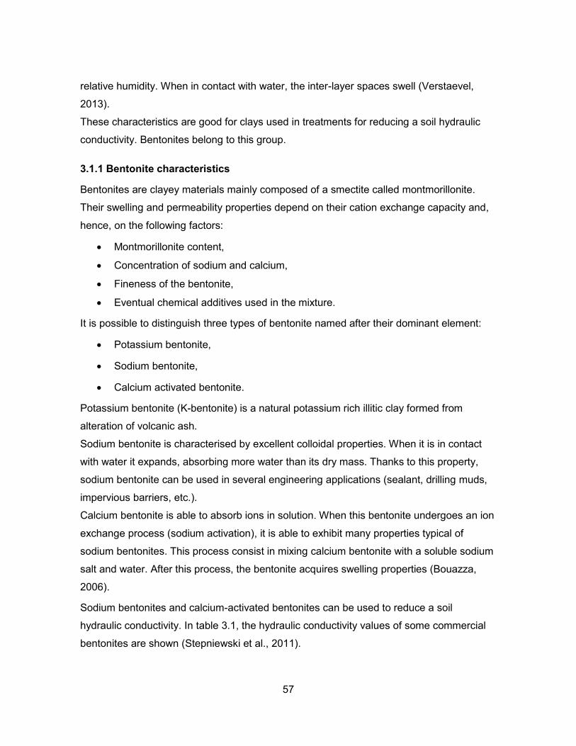
57
relative humidity. When in contact with water, the inter-layer spaces swell (Verstaevel,
2013).
These characteristics are good for clays used in treatments for reducing a soil hydraulic
conductivity. Bentonites belong to this group.
3.1.1 Bentonite characteristics
Bentonites are clayey materials mainly composed of a smectite called montmorillonite.
Their swelling and permeability properties depend on their cation exchange capacity and,
hence, on the following factors:
Montmorillonite content,
Concentration of sodium and calcium,
Fineness of the bentonite,
Eventual chemical additives used in the mixture.
It is possible to distinguish three types of bentonite named after their dominant element:
Potassium bentonite,
Sodium bentonite,
Calcium activated bentonite.
Potassium bentonite (K-bentonite) is a natural potassium rich illitic clay formed from
alteration of volcanic ash.
Sodium bentonite is characterised by excellent colloidal properties. When it is in contact
with water it expands, absorbing more water than its dry mass. Thanks to this property,
sodium bentonite can be used in several engineering applications (sealant, drilling muds,
impervious barriers, etc.).
Calcium bentonite is able to absorb ions in solution. When this bentonite undergoes an ion
exchange process (sodium activation), it is able to exhibit many properties typical of
sodium bentonites. This process consist in mixing calcium bentonite with a soluble sodium
salt and water. After this process, the bentonite acquires swelling properties (Bouazza,
2006).
Sodium bentonites and calcium-activated bentonites can be used to reduce a soil
hydraulic conductivity. In table 3.1, the hydraulic conductivity values of some commercial
bentonites are shown (Stepniewski et al., 2011).

58
Table 3.1
However, for a more detailed analysis of the hydraulic conductivity values of bentonites,
ageing process in situ should be considered. In fact, if cation exchange occurs, sodium
cations could be replaced by other cations and this process could affect the hydraulic
conductivity (Aldaeef et al., 2014).
3.2 EFFECT OF BENTONITE TREATMENTS ON SOIL PROPERTIES
In this paragraph the effect of bentonite on the treated soils will be discussed referring to
the studies by Couradin et al. (2008), Labiod-Aloui et al. (2014), Didier et al. (1996) and
BRGM (1992).
3.2.1 Atterberg’s limits
Labiod-Aloui et al. (2014) studied the effect of bentonite treatments on a sediment from the
Chorfa dam in Algeria, with the purpose of using them to realise an impermeable barrier
against the spread out of the “Sebkha of Oran” lake.
In figure 3.2, the granulometry of the Chorfa sediment and of the bentonite used for the
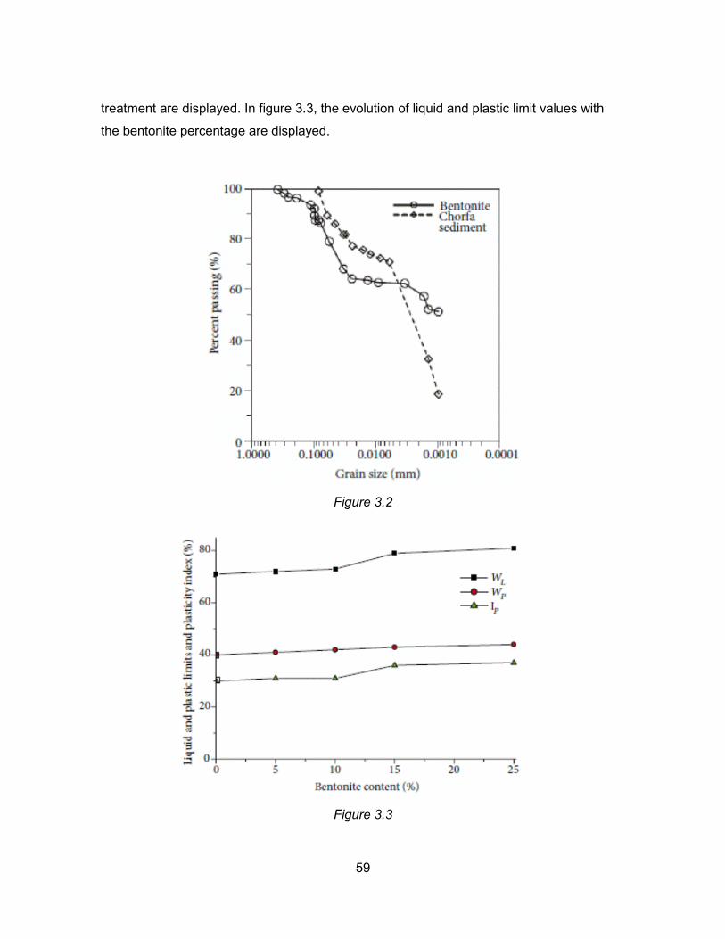
59
treatment are displayed. In figure 3.3, the evolution of liquid and plastic limit values with
the bentonite percentage are displayed.
Figure 3.2
Figure 3.3
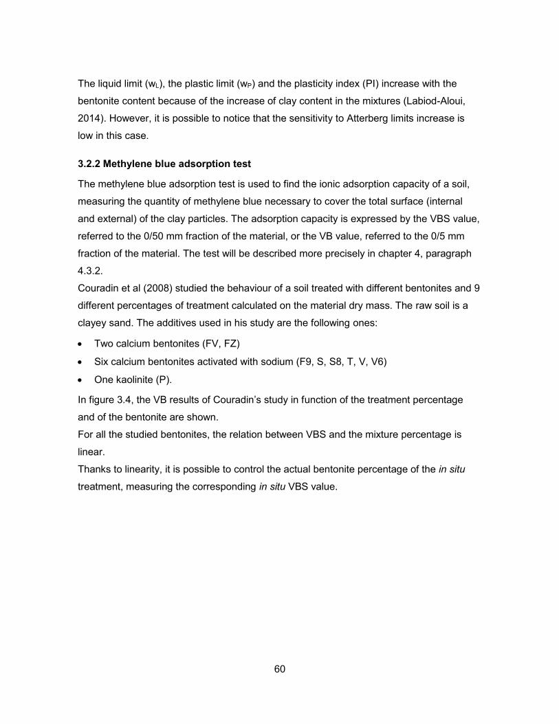
60
The liquid limit (wL), the plastic limit (wP) and the plasticity index (PI) increase with the
bentonite content because of the increase of clay content in the mixtures (Labiod-Aloui,
2014). However, it is possible to notice that the sensitivity to Atterberg limits increase is
low in this case.
3.2.2 Methylene blue adsorption test
The methylene blue adsorption test is used to find the ionic adsorption capacity of a soil,
measuring the quantity of methylene blue necessary to cover the total surface (internal
and external) of the clay particles. The adsorption capacity is expressed by the VBS value,
referred to the 0/50 mm fraction of the material, or the VB value, referred to the 0/5 mm
fraction of the material. The test will be described more precisely in chapter 4, paragraph
4.3.2.
Couradin et al (2008) studied the behaviour of a soil treated with different bentonites and 9
different percentages of treatment calculated on the material dry mass. The raw soil is a
clayey sand. The additives used in his study are the following ones:
Two calcium bentonites (FV, FZ)
Six calcium bentonites activated with sodium (F9, S, S8, T, V, V6)
One kaolinite (P).
In figure 3.4, the VB results of Couradin’s study in function of the treatment percentage
and of the bentonite are shown.
For all the studied bentonites, the relation between VBS and the mixture percentage is
linear.
Thanks to linearity, it is possible to control the actual bentonite percentage of the in situ
treatment, measuring the corresponding in situ VBS value.

61
Figure 3.4
3.2.3 Compaction properties
The compaction properties of a soil can be analysed through the compaction curve (γd, w)
obtained with Proctor procedure.
In the study already introduced in paragraph 3.2.2, Couradin et al. (2008) analysed the
compaction characteristics of the treatments with the standard Proctor procedure
according to the French norm NF P 94-093.
In figure 3.5, the results are displayed. The continuous curve is the compaction curve of
the raw material (clayey sand - Sm), while the symbols represent the couples (γd max, wOPT)
of each treatment (S, T, V, FV, FZ, S8, F9, P, V6).
It is possible to observe that all the treated samples are characterised by higher dry unit
weights.

62
Figure 3.5
In the study already introduced in paragraph 3.2.1, Labiod-Aloui et al. (2014) obtained the
compaction curves of the analysed soils.
Another example of variation of the compaction characteristics of soils treated with
bentonite is displayed in figure 3.6 and figure 3.7 (Labiod-Aloui et al., 2014).

63
Figure 3.6
Figure 3.7
Also in this case, with the increase of bentonite content, the maximum dry unit weight
increases and the optimum water content decreases.
In general, if a soil is mixed with fine material, γd,max increases and wOPT decreases. This is
due to the bentonite filling the porosities between the coarse particles.
However, it must be considered that the finer the granulometry of a soil, the lower the γd max

64
and the higher the wOPT, as shown in figure 3.8 (Colombo, 2004).
Therefore, if the bentonite treatment is used on a fine soil, the addition could contribute to
loosen the soil structure, leading to a decrease of the dry unit weight.
Figure 3.8
3.2.4 Hydraulic conductivity
The addition of a certain percentage of bentonite diminishes significantly the hydraulic
conductivity of a soil, as shown in figure 3.9 (Didier et al., 1996).
Figure 3.9

65
In figure 3.10, the results by Couradin et al. (2008) are displayed. The analysed soils are
always the ones already presented in paragraph 3.2.2: a clayey sand treated with different
types of additives (6 calcium-activated bentonites, 2 calcium bentonites, 1 kaolinite).
The hydraulic conductivity values were obtained with the rigid wall oedo-permeameter (NF
X 30-441) performed on the samples compacted with the standard Proctor procedure at
the optimum water content.
The hydraulic conductivity of the raw material is 1.6∙10-6 m/s and the addition of bentonite
provokes a consistent decrease of hydraulic conductivity for all the studied treatments.
It is possible to notice that in order to reach a hydraulic conductivity of at least 10-9 m/s, the
necessary percentage of calcium activated bentonites (F9, S, S8, T, V, V6) is minor than
the necessary percentage of the natural calcium bentonites (FV, FZ).
Figure 3.10
In 1992 BRGM (Bureau de Recherches Geologiques et Minieres), published a study on
the effect of bentonite treatments on a soil characterised by low hydraulic conductivity.
All the hydraulic conductivity measures were obtained with the oedo-permeameter test,

66
performed on samples compacted with the standard Proctor procedure at different water
contents.
The hydraulic conductivity of the raw material is comprised in the range [2∙10-8, 1∙10-9] m/s.
For the treatments, three percentages of bentonite treatments were used: 4%, 7%, 10% of
the dry mass. The hydraulic conductivities of the treated materials are comprised in the
range [1,5∙10-10, 5∙10-10] m/s.
In figure 3.11, the results of the study are displayed (BRGM, 1992). The lowest hydraulic
conductivity was obtained with the 10% treatment, which is the highest bentonite content
among the ones analysed by BRGM (1992). However, it is possible to notice that the
difference between the hydraulic conductivities obtained with different treatments is not
remarkable.
Figure 3.11
In the study already introduced in paragraph 3.2.1, Labiod-Aloui et al. (2014) obtained the
variation of the vertical and horizontal hydraulic conductivity in function of the bentonite
used for the treatment on the raw soil.
The vertical hydraulic conductivity values were obtained using compaction permeameter
(mould with the same dimensions as the Proctor mould). The samples were compacted
with the standard Proctor procedure at the optimum water content according to the French

67
norm NF P 94-093. The upper and lower plates of the Proctor mould were replaced by the
compaction permeameter ones in order to allow the water flow through the sample. The
saturation phase lasted for a period of about 1,5to 2 months. Samples were considered
fully saturated when water was coming out of the water outlet portal of the compaction
permeameter equipment.
The horizontal hydraulic conductivity values were obtained using drainage and seepage
tank model HM 169. The equipment used for the measure is shown in figure 3.12 (Labiod-
Aloui et al., 2014).
Figure 3.12
The results obtained by Labiod-Aloui et al. (2014) are displayed in figure 3.13.
The untreated material vertical hydraulic conductivity is 2∙10-10 m/s. The higher the
bentonite content of the sample, the lower the hydraulic conductivity.

68
Figure 3.13
3.3 CONCLUSIONS ON BENTONITE TREATMENTS
The following major conclusions on the effect of bentonite treatments on the geotechnical
and hydraulic characteristics of a soil can be drawn:
The Atterberg’s limits values (liquid limit, plastic limit and plasticity index) increase
with the increase of bentonite content.
The VB (and VBS) value increases with the increase of bentonite content.
Depending on the raw soil fine fractions, the dry unit weight at optimum water
content can increase or decrease with the increase of bentonite content.
The hydraulic conductivity decreases as the bentonite content increases but the
efficiency of the treatment depends on the raw soils characteristics.

69
CHAPTER 4 The CSM, the characterisation of the soils of the CSM and their bentonite treatments
In this chapter, the Centre de Stockage de la Manche (CSM) will be introduced focusing in
particular on its history and its cap cover system.
The soils object of this study and the proposed bentonite treatments will be described and
characterised through a series of classic geotechnical tests (Granulometry, VBS, Atterberg
limit, Proctor, water pycnometer, etc.).
The results of these tests will be discussed, highlighting the effect of the bentonite
treatments on the soil properties.
4.1 THE CENTRE DE STOCKAGE DE LA MANCHE (CSM)
The Centre de Stockage de la Manche (CSM) is a surface disposal facility for average and
low radioactivity waste characterised by short life. It is located in the department of the
French region called Basse-Normandie (figure 4.1).
It consists in a surface of 15000 m2 and until the year of its closure, it had received 527225
m3 of average and low radioactivity waste (Verstaevel, 2013). The current appearance of
the CSM is displayed in figure 4.2.
Figure 4.1

70
Figure 4.2
4.1.1 History of the CSM
The CSM was opened in 1969, when it received the first package of radioactive waste,
and was closed in 1994 when it arrived at saturation after a total exploitation time of 25
years (Gourden, 1996). During this period, since the technologic progress in radioactive
waste management was continuous, it was necessary to adapt and improve the disposal
centre. Therefore, the following phases can be distinguished (ANDRA, 2009):
Initial phase (1969 - 1979).
Transitional phase (1979 - 1983).
Industrial phase (1983 - 1994).
Monitoring phase (1994 - 2003).
Long-term monitoring phase (2003 - Nowadays).
During the initial phase (1969-1979), the waste was compacted in concrete covered
barrels. These barrels were lain down in trenches excavated directly in the ground (figure
4.3). This method was subjected to several problems and, hence, was replaced by a better
solution: the storage of the barrels on platforms or in concrete trenches according to the

71
radioactivity level (figure 4.4). During this phase, the waste conditioning was progressively
improved and the controls on the radioactivity level became stricter.
In 1978, 100000 m3 of waste had already been stocked in the facility (ANDRA, 2009).
Figure 4.3
Figure 4.4
The beginning of the transitional phase (1979-1983) is marked by the creation of a national
agency for the radioactive waste management: the ANDRA (Agence nationale pour la
gestion des déchets radioactifs). This agency began to regulate the procedures of the
waste barrels manufacturing, the acceptable radioactivity limits in the facility, the waste
conditioning, etc.
During the industrial phase (1983-1994), the waste management was improved
introducing a series of regulations with the objective of controlling the radioactivity level
(registration of the barrels characteristics: content, dimensions, etc.). The barrels were
stored in cells made of reinforced concrete (monolith) (figure 4.5) and with a tumulus
disposition (figure 4.6). In particular, the waste that was disposed in the ground during the
first phase was retrieved and stored in the tumuli.
The water collecting system was improved separating the superficial water and the
infiltration one. At the beginning of the eighties, a facility to collect the infiltration water was
built, and, in 1991, the cap-cover system building started (ANDRA, 2009).

72
Figure 4.5 Figure 4.6
In 1994, the facility received its last waste package and the monitoring phase started
(1994-2003). The cap cover system was complete in 1997. Its main objective is to isolate
the radioactive waste from the external environment. The water collecting system was also
improved in order to collect superficial and infiltration water (ANDRA, 2009).
The characteristics of the cap cover system will be described in more detail in paragraph
4.1.2.
In 2003, the long-term monitoring phase (2003 - nowadays) started officially. The main
objective of this phase is to control the impact of the disposal facility on the environment,
to identify eventual problems and, hence, to provide proper resolutions to these problems.
This phase will last some centuries (ANDRA, 2009).
4.1.2 The cap cover system of the CSM
The installation of the cap cover system of the CSM took place from 1991 to 1997. It was
the first time in the world that a multi-layer cap cover system was used in a disposal facility
for nuclear wastes (ANDRA, 2009). The function of the cap cover system is to isolate the
radioactive waste stored with the tumulus system or with the monolith system. Therefore, it
is possible to distinguish the three following functions (ANDRA, 2009):
To prevent water from reaching the radioactive waste and, hence, from producing
leachate which could contaminate the groundwater and the environment near the
facility.

73
To protect the stored waste from the ground movements.
To protect the facility from human, animal and vegetal intrusion.
The cap cover configuration and composition are displayed in figure 4.7.
Figure 4.7
Layer 7 is the vegetative cover consisting of natural untreated soil. It has a protective
function against the meteorological agents.
Layer 6 consists of sandy loam with a protective function against human, animal and
vegetal intrusion.
Layer 5 consists of a sand layer with draining function. This layer collects the water
filtrating from the upper one (layer 6) and conveys it to a drainpipe situated at the lowest
point of the layer.
Layer 4 consists of an impermeable bituminous geomembrane with the function of
preventing water from seeping to the lower layers.
Layer 3 is equivalent to layer 5. Therefore, it is made of a draining sand layer, which
conveys to the drainpipes the eventual water leakage from the superior layers. This layer
is equipped with an alarm system, which activates when water leakage is detected.
Layer 2 consists in a bituminous geomembrane equivalent to layer 4. Its aim is to collect

74
the possible leakage from the upper geomembrane (layer 4).
Layer 1 is a sandy loam layer covering the radioactive waste. Its function is to give to the
cap cover the proper slope and hence, the “factory roof” shape selected in order to
facilitate the drainage in layer 5 and layer 3.
In table 4.1 the composition, the function and the thickness of each layer are presented.
LAYER Material Function Thickness
7 Natural soil Protection against
meteorological agents 0,15/0,30 m
6 Sandy Loam Protection
against intrusion 1,00/1,40 m
5 Sand Drainage 0,20 m
4 Bituminous
Geomembrane Impermeable
barrier 5 mm
3 Sand Drainage 0,20 m
2 Bituminous
Geomembrane Impermeable
barrier 5 mm
1 Sandy Loam Cap cover shape Variable
Table 4.1
4.1.3 The long term cap cover system
In 2012, a retrieving campaign was conducted on the superficial layer (sandy loam). All the
samples have been brought to the Laboratoire d’étude des transferts en hydrologie et
environnement (LTHE) to be classified and studied.
The purpose was the study of the hydraulic conductivity of the superficial part of the cap
cover system (layer 7 and layer 6) in order to consider a possible treatment to improve its
impermeability (ANDRA, 2012b) and let the CSM go from active protection conditions to
passive protection ones (Chapter 1 paragraph 1.3.1).
The treated soil should substitute in the future for half the superficial layer of the cap cover
system. This substitution could interest the upper half or the lower half.
In the first case the installation would be much easier, in the second case it would be a
more complex operation because of the risk of damaging the geomembrane and the need
of removing the upper soil, but more efficient.
In the following paragraphs, after introducing the soil in situ and the proposed treatments,
the tests performed to characterise these materials will be presented.

75
4.2 THE TYPE MATERIALS AND THEIR TREATMENTS
4.2.1 Definition of the type materials: T12 and T3
Since the CSM cap cover system was built in three different steps, the samples collected
with the sample taking campaign were distinguished in the following three groups (tranche)
(Verstaevel, 2013):
T1 (26 samples) – samples collected from the most ancient part of the cap cover
system (first step of its building); this group consists of in situ excavation material.
T2 (38 samples) – samples collected from the part corresponding to the second
step of the cap cover realisation; as T1, this group consists of in situ excavation
material.
T3 (36 samples) – samples collected from the part corresponding to the last step of
the cap cover realisation; this group consists of calibrated material coming from a
quarry.
The results of the granulometry, the methylene blue adsorption test and the Atterberg
limits, performed for each single sample of the three groups, showed that the first two
typologies of material (T1 and T2) have very similar properties. Therefore, since the
differences in the properties of T1 and T2 are not significant, a type material was prepared
blending the T1 and T2 samples. The obtained type material was called T12.
All the T3 samples were mixed too in order to obtain the T3 type material.
From now on, the appellations T12 and T3 will be used to indicate the type materials. In
figure 4.8 and figure 4.9 the aspect of the 0/5 mm fraction of T12 and T3 respectively are
displayed.
Figure 4.8
Figure 4.9

76
4.2.2 The bentonite treatments
The additive chosen for the treatment of type soils T12 and T3 is a calcium-activated
bentonite, belonging to the smectites family. The properties of this typology of bentonite
have already been described in chapter 3 paragraph 3.1.1.
The characteristics of the bentonite used for the treatments are presented in table 4.2.
IMPERSOL® Sv
Colour Pinkish powder
Medium swelling 14 ml/g
Specific weight 2,7 g/cm3
Apparent density 0,7 g/cm3
Passing at 75 μm sieve (dry) ≥ 75 %
Passing at 75 μm sieve (humid) ≥ 96 %
Water content 8 ÷ 14 %
Table 4.2
In order to study the influence of the addition of bentonite to the T12 and the T3, the
following percentages for the treatments were proposed:
T12 (or T3) + 5% of bentonite T12 5% (or T3 5%).
T12 (or T3) + 7% of bentonite T12 7% (or T3 7%).
T12 (or T3) + 12% of bentonite T12 12% (or T3 12%).
The percentage is calculated on the dry mass of the 0/5 mm fraction of the type material
(T12 or T3).
The 7% bentonite treatment is the most eligible to be used effectively in the CSM for the
long-term cap cover system. However, the three values were considered in order to find
correlations between the bentonite content and the soils properties, focusing in particular
on the hydraulic ones.
4.3 CLASSIFICATION OF THE SOILS
In this paragraph, the soils introduced in paragraph 4.1 will be characterised with the help
of the French norm NF P 11-300 (1992).
Therefore, after presenting the granular distributions, the methylene blue adsorption test
and the Atterberg limits respectively in paragraph 4.2.1 paragraph 4.2.2 and paragraph
4.2.3, the classification will be presented (paragraph 4.2.4)
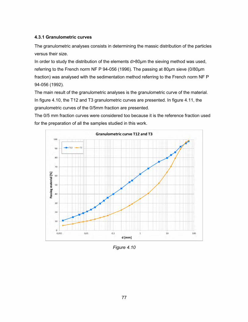
77
4.3.1 Granulometric curves
The granulometric analyses consists in determining the massic distribution of the particles
versus their size.
In order to study the distribution of the elements d>80µm the sieving method was used,
referring to the French norm NF P 94-056 (1996). The passing at 80µm sieve (0/80µm
fraction) was analysed with the sedimentation method referring to the French norm NF P
94-056 (1992).
The main result of the granulometric analyses is the granulometric curve of the material.
In figure 4.10, the T12 and T3 granulometric curves are presented. In figure 4.11, the
granulometric curves of the 0/5mm fraction are presented.
The 0/5 mm fraction curves were considered too because it is the reference fraction used
for the preparation of all the samples studied in this work.
Figure 4.10

78
Figure 4.11
From the granular distributions, it is possible to calculate two parameters: the uniformity
coefficient CU and the curvature coefficient CZ.
CU corresponds to the average slope of the curve with the vertical axis in the mean part:
𝐶𝑈 =𝑑60
𝑑10 (4.1)
Where d60 is the particle diameter (mm) corresponding to the 60% of the passing material
and d10 is the particle diameter (mm) corresponding to the 10% of the passing material.
When CU is in minor than 2, the soil has a uniform granulometry. When CU is higher than 2
the soil is characterised by a wide range of particles dimension (Verstaevel, 2013).
CZ measures the shape of the particle size curve and is calculated with the following
equation:
𝐶𝑍 =(𝑑30)2
𝑑60 ∙ 𝑑10 (4.2)

79
Where d30 is the particle diameter (mm) corresponding to the 30% of the passing material.
When CZ is between 1 and 3 the soil is well graded (Verstaevel, 2013).
Other two parameters used for the soils classification are the fine fraction FF (percentage
of passing material at the 80µm sieve) and dmax (the maximum dimension of the biggest
particles of the soil).
In table 4.3 the values of d10, d30, d60, dmax, FF, CU and CZ are displayed for the type
materials T12 and T3 considering the complete curves and the 0/5 mm fraction curves.
T12 T3
T12 (0/5mm)
T3 (0/5mm)
d10 [mm] 0,00124 0,00899 0,00093 0,00129
d30 [mm] 0,03429 0,58162 0,01439 0,05092
d60 [mm] 0,86096 8,34200 0,18594 0,68447
dmax [mm] 63,00 63,00 5,00 5,00
FF 37,92% 17,15% 50,20% 33,01%
CU 696,71 927,43 199,21 529,76
CZ 1,11 4,51 1,19 2,93
Table 4.3
The T12 results a well-graded soil considering both the complete curve and the 0/5mm
fraction (CU>2 and 1<CZ<3).
The T3 results a bad-graded soil if the complete curve is considered (CU>2 and CZ>3) and
a well-graded soil if the 0/5mm fraction is considered (CU>2 and 1<CZ<3).
Regarding the treated soils granulometries, they were not analysed with the sieving and
the sedimentation method. However, it is possible to find the fine fraction FF (d<80µm) of
each treatment considering that the bentonite consists in particles inferior to 80µm (table
4.2).
The values of FF for each treatment distinguishing between the complete curve and the
0/5mm fraction are displayed in table 4.4.

80
T12 T3 T12
(0/5mm) T3
(0/5mm)
0% 37,92% 17,15% 50,20% 33,01%
5% 40,88% 21,10% 52,57% 36,20%
7% 41,98% 22,57% 53,46% 37,39%
12% 44,57% 26,03% 55,54% 40,19%
Table 4.4
Because of the bentonite treatment, the fine fraction FF increases. This effect is obviously
more visible if the 0/5mm fraction only is considered.
4.3.2 Methylene blue adsorption test (VBS)
The methylene blue adsorption test is used to find the ionic adsorption capacity of a soil,
measuring the quantity of methylene blue necessary to cover the total surface (internal
and external) of the clay particles. The test is performed on samples obtained from the 0/5
mm fraction as explained in the French norm NF P 94-068.
The adsorption capacity is expressed by the VBS value, from the French Valeur de Bleu
du Sol, (grams of methylene blue absorbable by 100 grams of dry soil) referred to the 0/50
mm fraction of the material.
VBS is calculated with the following equation (NF P 94-068):
𝑉𝐵𝑆 = 𝐶 ∙ 𝑉𝐵 [0 50 𝑚𝑚⁄ ] (4.3)
Where C is the proportion of the 0/5 mm fraction in the 0/50 mm fraction of the dry
material, and VB is the adsorption capacity of the soil (grams of methylene blue
absorbable by 100 grams of dry soil) referred to the 0/5 mm fraction.
The VB is calculated from the test results with the following equation:
𝑉𝐵 =𝐵
𝑚𝑑∙ 100 [0 5 𝑚𝑚]⁄ (4.4)
Where B is the methylene blue mass used in the test (g) and md is the dry mass of the
sample (g).
The VB and VBS calculated from the test results are presented in table 4.5.

81
T12 T3 0% 5% 7% 12% 0% 5% 7% 12%
VB [0/5 mm] 0,96 2,22 2,88 4,41 0,65 2,04 2,37 3,45 VBS [0/50 mm] 0,72 1,69 2,20 3,40 0,34 1,08 1,27 1,89
Table 4.5
The higher the bentonite percentage, the higher the value obtained from the test. This
happens because the bentonite contributes to increase the clay fraction of the starting
soils (T12 and T3) making the mix more reactive and capable of absorbing the methylene
blue. In fact, the bentonite is the clay with the extreme specific area.
Moreover, it is possible to observe that T12 and all its treatments are characterised by
higher VB and VBS values than the corresponding ones of the T3 based soils. In fact, T12
clay fraction (0/2 µm) is higher than T3 one and, hence, this makes T12 based soils more
reactive.
These considerations can also be deduced observing the graphic in figure 4.12, which
represents the VB in function of the bentonite percentage.
Figure 4.12

82
The two lines plotted in figure represent the linear correlation between VB and the
bentonite percentage of the treatment, respectively for T12 based and T3 based soils.
It is possible to verify that the linear correlation found by Couradin and others (2008)
(Chapter 3 paragraph 3.2.2) is valid for the soils studied in this work.
Thanks to the existence of a linear correlation between VB (or VBS) and the bentonite
percentage of the treatment, it is possible to make valid hypothesis on the VB (and VBS)
values of T12 and T3 treated with bentonite percentages not directly studied with the
methylene blue test. Moreover, thanks to linearity, it is possible to control the actual
bentonite percentage of the in situ treatment, measuring the corresponding in situ VBS
value.
4.3.3 Atterberg limits
The liquid limit (wL), the plastic limit (wP) and the plasticity index (PI) were found for all the
untreated and treated soils referring to the French norm NF P 94-051 (1993). This
standard is applied to the soil fraction passing at the 400 µm sieve (0/400µm fraction).
The liquid limit wL is the soil water content corresponding to the transition point between
liquid and plastic behaviour. Experimentally, it corresponds to the water content at which a
groove made on a soil placed in the Casagrande cup closes when the cup undergoes 25
repeated drops from a 10 mm height (NF P 94-051, 1993).
The plastic limit wP is the soil water content corresponding to the transition point between
plastic and solid behaviour. Experimentally, it corresponds to the water content at which a
thread of soil breaks apart having a diameter of 3 mm ±0,5 mm (NF P 94-051, 1993).
The plasticity index PI is the difference between the liquid limit and the plastic limit:
𝑃𝐼 = 𝑤𝐿 − 𝑤𝑃 (4.5)
All the three parameters are expressed in percentage format.
The test were performed at least two times for all the analysed soils. In particular, for the
untreated soils, the tests were performed on 64 samples for T1+T2 (26 samples of T1 and
38 samples of T2) and on 36 samples for T3.
The results were calculated as average values.
In table 4.6 and figure 4.13, the results are presented.

83
T12 T3 0% 5% 7% 12% 0% 5% 7% 12%
wL 31,25% 53,74% 76,00% 110,35% 32,50% 52,87% 63,24% 109,23%
wP 21,87% 22,30% 27,13% 35,10% 22,81% 23,59% 27,70% 33,33% PI 9,38% 31,44% 48,87% 75,25% 9,69% 29,27% 35,54% 75,90%
Table 4.6
Figure 4.13
In figure 4.13 the dotted lines correspond to the average values of Atterberg limits
obtained from the 64 samples of T1+T2 and the 36 samples of T3.
In first place, it is evident that the higher the bentonite content, the higher the Atterberg
limits. In particular, it is possible to notice that the liquid limit is subjected to a more

84
important increase than the plastic limit. Therefore, the resulting plasticity index increases
significantly with the bentonite percentage, as it is shown in figure 4.14.
Figure 4.14
In second place, it is possible to notice that the T12 and T3 do not show important
differences in the Atterberg limits values with the exception of the liquid limit at 7% of
bentonite. However, this exception could be explainable as a consequence of an
overestimation of the liquid limit of T12 7%. In fact, the Atterberg limits estimation is always
exposed to errors due to the operator’s subjectivity and the water content measures.
Finally, the GTR (Guide des Terrassements Routiers) provides the following criteria to
judge the influence of the Atterberg limits on the soil behaviour (GTR, 1992):

85
If the 0/400 µm fraction is more than the 50% of the complete granulometric curve
and PI is higher than 12%, the results are realistic and can be used to describe the
soil behaviour.
If the 0/400 µm fraction is less than the 35% of the complete granulometric curve
and PI is lower than 6%, the results cannot be interpreted.
All the 0/5 mm fractions of the soils analysed in this work are characterised by a 0/400 µm
fraction forming more than the 50% of the granulometric curve. The PI is always higher
than 12% with the exception of the untreated soils, T12 and T3, for which it is between 9%
and 10%.
Therefore, according to the GTR indications, the obtained results for the Atterberg limits
can be considered sufficiently reliable.
The liquid limit and the plasticity index obtained for each soil, were used to find the
corresponding point in the Casagrande’s chart.
In figure 4.15, the Casagrande’s chart is presented.
Figure 4.15

86
The soils are always in the field of inorganic clays. Given the bentonite percentage, the
positions in the chart of T12 based soils and T3 based ones are very similar. The only
exception is the 7% percentage for the reasons already explained previously.
It is possible to point out that, increasing the soil bentonite content, the soil plasticity
increases consistently:
T12 0% and T3 0% are low plasticity clays.
T12 5% and T3 5% are medium plasticity clays.
T12 7% and T3 7% are high plasticity clays.
T12 12% and T3 12% are very high plasticity clays.
4.3.4 Classification of the samples
The results presented in the previous paragraphs will be used to classify the soils with the
use of the French standard NF P 11-300 (1992).
Since all the tests were performed on samples obtained from the 0/5mm fraction of the
soils, the soils were classified referring to the same fraction.
The standard classifies the soils according to the following characteristics:
The granulometric curve, in particular the dmax (maximum dimension of the soil
grains) and the fine material fraction FF (percentage of particles with dimensions
inferior to 80 µm).
The plastic index (PI).
The methylene blue adsorption value referred to the 0/5mm fraction (VB).
In table 4.7, the NF P 11-300 tables used for the classification are presented.
In table 4.8 the properties used for the classification are presented.

87
Table 4.7
dmax [mm] FF PI VB
T12 0/5mm
0% 5,00 50,20% 9,38% 0,96 A1
5% 5,00 52,57% 31,44% 2,22 A3
7% 5,00 53,46% 48,87% 2,88 A4
12% 5,00 55,54% 75,25% 4,41 A4
T3 0/5mm
0% 5,00 33,01% 9,69% 0,65 B5
5% 5,00 36,20% 29,27% 2,04 A3
7% 5,00 37,39% 35,54% 2,37 A3
12% 5,00 40,19% 75,90% 3,45 A4
Table 4.8
Hence, the 0/5mm fractions of the studied soils can be classified as following:
T12 0% - Low plasticity silt (A1).
T12 5% - High plasticity silt (A3).
T12 7% - High plasticity clay (A4).
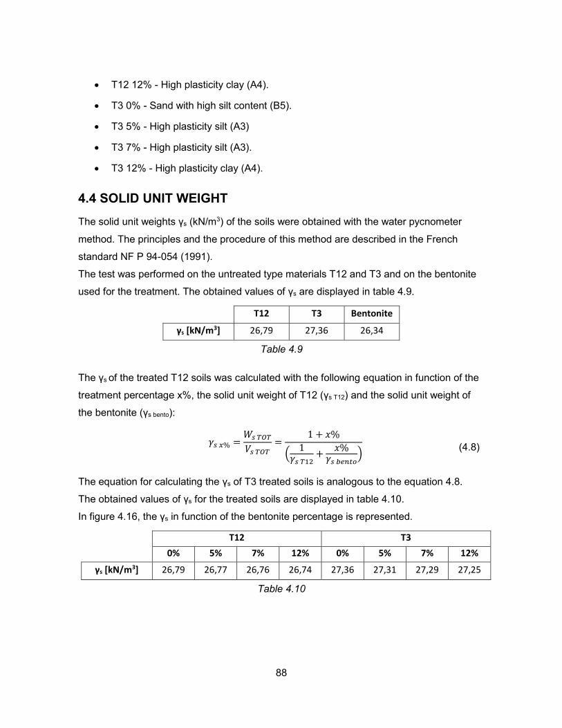
88
T12 12% - High plasticity clay (A4).
T3 0% - Sand with high silt content (B5).
T3 5% - High plasticity silt (A3)
T3 7% - High plasticity silt (A3).
T3 12% - High plasticity clay (A4).
4.4 SOLID UNIT WEIGHT
The solid unit weights γs (kN/m3) of the soils were obtained with the water pycnometer
method. The principles and the procedure of this method are described in the French
standard NF P 94-054 (1991).
The test was performed on the untreated type materials T12 and T3 and on the bentonite
used for the treatment. The obtained values of γs are displayed in table 4.9.
T12 T3 Bentonite
γs [kN/m3] 26,79 27,36 26,34
Table 4.9
The γs of the treated T12 soils was calculated with the following equation in function of the
treatment percentage x%, the solid unit weight of T12 (γs T12) and the solid unit weight of
the bentonite (γs bento):
𝛾𝑠 𝑥% =𝑊𝑠 𝑇𝑂𝑇
𝑉𝑠 𝑇𝑂𝑇=
1 + 𝑥%
(1
𝛾𝑠 𝑇12+
𝑥%𝛾𝑠 𝑏𝑒𝑛𝑡𝑜
) (4.8)
The equation for calculating the γs of T3 treated soils is analogous to the equation 4.8.
The obtained values of γs for the treated soils are displayed in table 4.10.
In figure 4.16, the γs in function of the bentonite percentage is represented.
T12 T3
0% 5% 7% 12% 0% 5% 7% 12%
γs [kN/m3] 26,79 26,77 26,76 26,74 27,36 27,31 27,29 27,25
Table 4.10

89
Figure 4.16
The higher the bentonite content of the treated soil, the lower the solid unit weight of the
material. This effect is equivalent for T12 and T3 since the two lines are parallel.
4.5 PROCTOR TEST
The normal Proctor test was performed on the untreated and treated materials in order to
find the optimum water content wOPT and the maximum dry specific weight γd OPT. The
standard procedure, described in the French norm NF P 94-093 (1999), was used.
The test consists in humidifying a soil in order to have different water contents and to
compact it with a predetermined number of blows from a standard weighted hammer at a
specified height, for each water content.
Hence, for each water content, it is possible to find the dry unit weight of the material and
to trace the Proctor curve of the soil, which describes the variations of the dry unit weight

90
with the water content.
The test can be performed with either the Proctor or the CBR mould. The first is used
when dmax<5mm the second when dmax>5mm. Since the test was performed on samples
obtained from the 0/5mm fraction, the Proctor mould was used.
The mould diameter dmould, the mould height hmould, the mould volume Vmould, the hammer
weight Whammer, the fall height of the hammer H, the number of compacted layers in the
mould nl, the number of blows for each layer nb/l and the compaction energy E are
presented in table 4.11.
The compaction energy E is calculated with the following equation:
𝐸 =𝑚ℎ𝑎𝑚𝑚𝑒𝑟 ∙ 𝐻 ∙ 𝑛𝑙 ∙ 𝑛𝑏/𝑙
𝑉𝑚𝑜𝑢𝑙𝑑 (4.9)
dmould [m] 0,1015
hmould [m] 0,1165
Vmould [m3] 0,000942644
Whammer [N] 24,90
H [m] 0,305
nl 3
nb/l 25
E [N/m2] 604244
Table 4.11
From the Proctor curve, it is possible to acquire the maximum value of the dry unit weight
(γd OPT), which is obtained at a particular water content value called optimum water content
(wOPT).
In order to obtain a proper Proctor curve, a minimum of 5 points corresponding to 5
different water contents is required. In particular, in this work a minimum of 6 water
contents was used for each soil, in order to have 3 water contents minor than the optimum
and 3 superior to the optimum.
In figure 4.17 and figure 4.18, the Proctor curves of T12 based soils and T3 based ones,
respectively, are presented. In table 4.12 the values of wOPT and γd OPT are presented for
the analysed soils.

91
Figure 4.17
Figure 4.18

92
T12 T3
0% 5% 7% 12% 0% 5% 7% 12%
wOPT 12,3% 14,9% 16,4% 17,6% 11,1% 14,2% 15,0% 15,2%
d [kN/m3]
19,1 18,0 17,9 17,2 19,7 18,9 18,4 17,8
Table 4.12
The saturation curves equations represented in figure 4.17 and 4.18 are referred to the
untreated materials, respectively T12 and T3, and are obtained from the following equation
after fixing the degree of saturation S to 80% or 100% (Colombo, 2004):
𝛾𝑑 =𝑆 ∙ 𝛾𝑠
𝑆 ∙ 𝛾𝑤 + 𝑤 ∙ 𝛾𝑠 (4.10)
Where γs is the solid unit weight (kN/m3) of T12 0% or T3 0% (table 4.9 paragraph 4.4).
It is possible to find out that the maximum dry unit weight of the two type soils T12 and T3
gets lower as the bentonite percentage of the treatment increases.
This result is in contrast with the studies by Couradin et al. (2008) and Labiod-Aloui et al.
(2014) (Chapter 3 paragraph 3.2.3).
However, this could be due to the high fine content of the untreated type materials T12
and T3. In fact, as already outlined in chapter 3 paragraph 3.2.3, the addition of bentonite
to a fine soil can contribute to loosen the soil structure, leading to a decrease of the dry
unit weight.

93
4.6 SUMMARY OF THE SAMPLES CHARACTERISATION
In table 4.13, the parameters characterising the 0/5mm fraction of the soils under analysis
are displayed. In the following chapters, these results will be used in order to study the
variation of the hydraulic conductivity in function of the bentonite treatment.
T12 (0/5mm fraction) T3 (0/5mm fraction)
0% 5% 7% 12% 0% 5% 7% 12%
NF P 11-300 Classification A1 A3 A4 A4 B5 A3 A3 A4
VB 0,96 2,22 2,88 4,41 0,65 2,04 2,37 3,45
wL 31,25% 53,74% 76,00% 110,35% 32,50% 52,87% 63,24% 109,23%
wP 21,87% 22,30% 27,13% 35,10% 22,81% 23,59% 27,70% 33,33%
PI 9,38% 31,44% 48,87% 75,25% 9,69% 29,27% 35,54% 75,90%
γs [kN/m3] 26,79 26,77 26,76 26,74 27,36 27,31 27,29 27,25
wOPT 12,3% 14,9% 16,4% 17,6% 11,1% 14,2% 15,0% 15,2%
d [kN/m3] 19,1 18,0 17,9 17,2 19,7 18,9 18,4 17,8
Table 4.13
It must be outlined that, even if all the characterisation tests were performed on the 0/5
mm fraction of the soils, the in situ coarser fraction (complete granulometry) is not
negligible. Hence, the coarse fraction could have a certain influence on mechanical and
hydraulic properties of the analysed soils.
However, since the bentonite generally interacts with the 0/5 mm fraction of a soil, the
analysis in the following chapters are based on the 0/5 mm fractions properties.
The difference between the 0/5 mm fraction and the complete granulometry will be
considered for the internal erosion criteria applied to T12 0% and T3 0% in chapter 7.

94

95
CHAPTER 5 Influence of the treatments on hydraulic conductivity in saturated conditions
In this chapter the saturated hydraulic conductivity of T12, T3 and their bentonite
treatments will be calculated using the oedo-permeameter test and some correlations with
the soil properties.
After having described and applied each method, the results will be commented referring
to the reliability of each method.
In particular, the main interest is to assess the efficiency of bentonite treatments on the
impermeability of T12 and T3.
5.1 OEDO-PERMEAMETER TEST
5.1.1 Samples preparation
The samples used in the oedo-permeameter tests have been prepared mixing the 0/5 mm
fraction of the material with water to obtain the chosen water content. After the mixing, the
material undergoes a maturation for 72 hours minimum. This phase is necessary for
materials with a high fine content in order to have a water content perfectly homogeneous.
After compacting the material with normal Proctor procedure (Chapter 4 paragraph 4.5),
the samples have been obtained coring the soil directly with the cutting ring of the
oedometric cell. The advantage of this procedure is that it is possible to have a perfect
contact between the sample and the cell (Verstaevel, 2013).
Regarding the choice of the water content for the compaction, the indications of the
Bureau de Recherche Géologiques et Minières (BRGM) have been followed (Chapter 1,
paragraph 1.4.3). Hence, a gravimetric water content of wOPT+2% was chosen.
The calculation of wOPT+2% and γd OPT+2% will be discussed more in detail in reference to
the preparation of the hanging column test samples (chapter 6, paragraph 6.2.1).
In table 5.1, the calculated values of wOPT+2% and γd OPT+2% values are displayed.

96
wOPT+2% REAL
d OPT+2% [kN/m3]
T12 0% 14,29% 18,77
T12 5% 17,91% 17,51
T12 7% 19,73% 16,92
T12 12% 21,36% 16,47
T3 0% 12,63% 19,46
T3 5% 16,77% 18,13
T3 7% 17,40% 17,95
T3 12% 18,38% 17,40
Table 5.1
5.1.2 Description of the method
The hydraulic conductivity in laboratory is measured in saturated conditions and steady
state. Moreover, since temperature influences the viscosity of water and hence the
measure of hydraulic conductivity, the laboratory test have to be performed at constant
temperature, in general 20°C.
The test is based on the validity of Darcy’s law (chapter 2, paragraph 2.2.1):
𝑣 = 𝐾 ∙ 𝑖 (5.1)
Where v is the velocity of the permeant through the soil matrix (m/s), K is the hydraulic
conductivity (m/s) and i is the hydraulic gradient, calculated as following:
𝑖 =∆ℎ
𝐻 (5.2)
Where Δh is the difference of hydraulic charge between the upper and the lower part of the
sample (m) and H is the drainage distance of the sample in the flow direction (m).
Using the Darcy’s law it is possible to write the continuity equation with the following
expression:
𝑄 = 𝑣 ∙ 𝐴 = 𝐾 ∙ 𝑖 ∙ 𝐴 (5.3)
Where Q is the flow rate through the sample (m3/s).
Knowing the water volume V (m3) which passes through the sample in a time interval Δt (s)
it is possible to calculate the corresponding flow rate Q:

97
𝑄 =𝑉
∆𝑡 (5.4)
Substituting the equation 5.4 in the equation 5.3, the hydraulic conductivity can be found:
𝐾 =𝑉
𝐴 ∙ 𝑖 ∙ ∆𝑡 (5.5)
The measure of hydraulic permeability through the permeameter test can be done with two
methods:
Constant head test;
Falling head test.
In the constant head test the sample is subjected to a vertical flow imposed by a water
charge maintained constant during the test. This method assumes laminar flow conditions
and independency between the hydraulic conductivity and the hydraulic gradient.
Generally, the constant charge method is used for coarse-grained soils.
In the falling head test the sample is subjected to a vertical flow imposed by a variable
water charge. This method is used for both coarse-grained and fine-graded soils.
In this work rigid wall permeameters with the falling head procedure have been adopted.
The tests were performed referring to the French norm NF X 30-441 (1998). In these tests,
the samples are placed between two porous plates (one over and one under the sample)
in an oedometric cell, which blocks horizontal and vertical dilatations.
The test is organised in three phases according to the French norm NF X 30-442 (1998):
1st Phase.
The confinement charge is applied;
2nd Phase.
The sample is saturated applying a hydraulic charge until the steady state is
reached.
3rd Phase.
The interval of time Δt necessary to the loss of hydraulic charge Δh is measured.
Finally, it is possible to obtain the hydraulic conductivity K for each interval with the
following expression:

98
𝐾 =𝐻 ∙ 𝑠
𝐴 ∙ (𝑡1 − 𝑡0)𝑙𝑛 (
ℎ0
ℎ1) (5.6)
Where H is the drainage length of the sample in the flow direction and, hence, the height
of the sample (m), s is the section area of the tube providing water supply (m²), h0 and h1
(m) are the water heights in the supply tube respectively at time t0 and t1 (s).
In this work, the tests have been performed using a confinement of 26 kPa, corresponding
to a layer of soil characterised by a thickness slightly superior to 1 m, and a hydraulic
charge of 10 cm.
5.1.3 Results
The values of the hydraulic conductivities in saturated conditions are displayed in figure
5.1 and table 5.2.
Figure 5.1

99
KSAT [m/s] R
T12
0% 6,70E-10 -
5% 5,60E-10 16%
7% 1,50E-10 78%
12% 1,30E-10 81%
T3
0% 9,60E-10 -
5% 5,40E-10 44%
7% 2,60E-10 73%
12% 2,40E-10 75%
Table 5.2
The R value in table 5.2 can be used as a parameter to evaluate the efficiency of the
bentonite treatment. It indicates the reduction of hydraulic conductivity referred to the raw
material and is calculated with the following expression:
𝑅 =𝐾𝑆𝐴𝑇 (𝑢𝑛𝑡𝑟) − 𝐾𝑆𝐴𝑇 (𝑡𝑟)
𝐾𝑆𝐴𝑇 (𝑢𝑛𝑡𝑟) % (5.7)
The bentonite treatment contributes to decrease significantly the hydraulic conductivity of
the raw materials.
Referring to R values, it is possible to notice that the bentonite treatment tends to reach
the maximum of its effectiveness at 7%, since increasing the bentonite rate to 12%
produces an additional decrease of hydraulic conductivity, which is not sufficient to justify
the bentonite content increase.
In figure 5.2, the logarithmic value of KSAT is represented in function of the bentonite
content.
From figure 5.1 and figure 5.2, it is possible to notice that there is not an evident linear
correlation between the hydraulic conductivity measured with the oedo-permeameter and
the bentonite percentage of the treatment.

100
Figure 5.2
5.2 CORRELATIONS BETWEEN KSAT AND SOIL PROPERTIES
Different authors have tried to find a relation between hydraulic conductivity, and the
parameters that describe the nature of the soil (Magnan, 2000).
In the following paragraphs, some of these approaches will be applied on the studied soils.
In paragraph 5.2.1, three equations thought for sandy materials will be applied to the
untreated soils, T12 and T3.
In paragraph 5.2.2, the Sivakumar correlation, thought for cohesive materials, will be
applied to analyse the effect of the bentonite treatment.
The analysis will be referred to the 0/5 mm fraction of the materials. In particular, the
reference diameter d10 and d15 will be used; d10 and d15 are the diameters in m

101
corresponding to, respectively, the 10% and 15% of cumulative passant in the
granulometric curve.
All the applied equations consider the compaction conditions of the materials using the
porosity value (n) or the void ratio value (e). The analysis will be referred to the results of
the standard Proctor tests performed on each soil with a water content equal to wOPT+2%
as suggested by BRGM (Chapter 1, paragraph 1.4.3).
Therefore, the porosity was calculated with the following equation:
Where γd OPT+2% is the dry unit weight calculated with the Proctor test and γs is the solid unit
weight (chapter 4, paragraph 4.4).
The void ratio can be directly calculated with the following equation:
𝑒 =𝑛
1 − 𝑛 (5.9)
In table 5.3, the values of d10, d15, γs, γd OPT+2%, n and e are displayed.
d10 [mm] d15 [mm] s
[kN/m3] d OPT+2% [kN/m3]
n e
T12
0% 0,00093 0,00156 26,79 18,77 0,3049 0,4386
5% - - 26,77 17,51 0,3515 0,5421
7% - - 26,76 16,92 0,3732 0,5954
12% - - 26,74 16,47 0,3901 0,6395
T3
0% 0,00129 0,00391 27,36 19,46 0,2793 0,3875
5% - - 27,31 18,13 0,3284 0,4889
7% - - 27,29 17,95 0,3353 0,5045
12% - - 27,25 17,40 0,3554 0,5514
Table 5.3
5.2.1 Untreated soils
In this paragraph, the hydraulic conductivity of the untreated soils, T12 and T3, will be
calculated using three correlations which are generally used to obtain the hydraulic
conductivity of cohesionless soils.
𝑛 = 1 −𝛾𝑑 𝑂𝑃𝑇+2%
𝛾𝑠 (5.8)

102
Kozeny (1927) proposed an expression to evaluate the hydraulic conductivity of granular
materials. This expression was refined by Carman in 1937 and 1956.
The authors represent the porous structure of the soil as a system of pipes characterised
by tortuosity and a little diameter (capillary model). The expression for the hydraulic
conductivity K (m/s) is the following:
𝐾 =1
𝑘0𝑇2𝑆02 ∙
𝛾𝑤
𝜇∙
𝑛3
(1 − 𝑛)² (5.10)
Where k0 is the pore shape factor, T is the tortuosity of the flow path, S0 is the specific
surface area of soil particle, μ is the dynamic viscosity of water (kg/(ms)), γw is the unit
weight of water (N/m3), n is the porosity of the soil.
Equation 5.10 is difficult to apply because it is necessary to evaluate two coefficients: k0
and T.
In order to apply the formula in a simpler way, different ways of calculating k0, T and S0
have been proposed. In this work the following form will be applied:
𝐾 =1
80∙ 𝑑10
2 ∙𝛾𝑤
𝜇∙
𝑛3
(1 − 𝑛)2 (5.11)
Where d10 is expressed in m.
Chapuis (2004) elaborated the following correlation for loose sands:
𝐾 = 0,0246 ∙ [𝑑10𝑒3
1 + 𝑒]
0,7825
= 0,0246 ∙ [𝑑10𝑛3
(1 − 𝑛)2]
0,7825
(5.12)
Where d10 is expressed in m.
Bezuijen (2010) proposed the following correlation, based on Kozeny and Carman’s
studies:
𝐾 =1
160∙ 𝑑15
2 ∙𝛾𝑤
𝜇∙
𝑛3
(1 − 𝑛)2 (5.13)
Where d15 is expressed in m.
In table 5.4 and in the semi-logarithmic graphic of figure 5.3, the results of the analysis are
displayed. The values obtained with the oedo-permeameter are shown too.

103
KSAT [m/s]
T12 0% T3 0%
Kozeny Carman 5,81E-09 9,69E-09
Chapuis 4,84E-08 5,60E-08
Bezuijen 8,13E-09 4,43E-08
Oedo-Permeameter 6,70E-10 9,60E-10
Table 5.4
Figure 5.3
The values obtained from the oedo-permeameter are used as a reference to evaluate the
reliability of the correlations. In fact, these values can be considered the most realistic
ones since they are obtained from a direct experimentation on the soils.
The oedo-permeameter gives the lowest values of hydraulic conductivity.
All the three correlations tend to overestimate the hydraulic conductivity of the soils. This is
mainly because these correlations were obtained from studies on cohensionless soils and
are not suitable for clayey soils (Mitchell, 1993).

104
However, Kozeny-Carman equation 5.11 gives results which are nearer to the oedo-
permeameter ones, with a difference of about an order of magnitude.
5.2.2 Treated soils
In this paragraph, the effect of bentonite treatments on the hydraulic conductivity of T12
and T3 will be analysed using the Sivakumar correlation.
Sivakumar proposed the following equation to calculate the hydraulic conductivity of
normally consolidated clays:
2,50 + 0,24 ∙ 𝑙𝑜𝑔𝐾 =𝑒
𝑒𝐿 (5.14)
Where e is the void ratio corresponding to the Proctor standard compaction at wOPT+2%
(table 5.2), eL is the void ratio of the soil with a water content equal to the liquid limit wL.
From equation 5.14, it is possible to obtain K:
𝐾 = 10^ (
𝑒𝑒𝐿
− 2.5
0.24) (5.15)
In order to calculate the eL, it is possible to suppose that at a water content equal to wL the
soil is saturated. When the soil is in saturation conditions the void volume is equal to the
water volume inside the soil, hence it is possible to calculate eL with the following equation:
𝑤𝐿 = 𝑒𝐿
𝛾𝑤
𝛾𝑠 (5.16)
Where γw is the water unit weight (kN/m3) and γs is the solid unit weight (kN/m3).

105
In table 5.5, the values of wL and eL are displayed.
wL eL
T12
0% 31,25% 0,8534
5% 53,74% 1,4665
7% 76,00% 2,0730
12% 110,35% 3,0079
T3
0% 32,50% 0,9064
5% 52,87% 1,4717
7% 63,24% 1,7592
12% 109,23% 3,0340
Table 5.5
In figure 5.4 and table 5.6, the results of equation 5.15 are displayed. In figure 5.4, the
hydraulic conductivity values obtained with the oedo-permeameter test (paragraph 5.1.3)
are also represented.
Figure 5.4

106
KSAT (Sivakumar)
[m/s]
T12 T3
0% 4,68E-09 2,82E-09
5% 1,22E-09 1,04E-09
7% 5,64E-10 6,55E-10
12% 2,80E-10 2,29E-10
Table 5.6
The difference between the results obtained with the oedo-permeameter and Sivakumar,
decreases significantly with the bentonite content increase.
If the hydraulic conductivity is plotted using logarithmic values (figure 5.5), it is possible to
notice that the results obtained with Sivakumar’s equation 5.15 are linearly correlated to
the bentonite percentage of the treatment.
Figure 5.5

107
5.3 SUMMARY OF RESULTS
In table 5.7, all the values of hydraulic conductivity obtained in the previous paragraphs
are displayed.
Oedo-
Permeameter Sivakumar
Kozeny Carman
Chapuis Bezuijen
T12
0% 6,70E-10 4,68E-09 5,80841E-09 4,8414E-08 8,1321E-09
5% 5,60E-10 1,22E-09 - - -
7% 1,50E-10 5,64E-10 - - -
12% 1,30E-10 2,80E-10 - - -
T3
0% 9,60E-10 2,82E-09 9,68712E-09 5,6012E-08 4,4344E-08
5% 5,40E-10 1,04E-09 - - -
7% 2,60E-10 6,55E-10 - - -
12% 2,40E-10 2,29E-10 - - -
Table 5.7
The reference values for the following chapters will be the oedo-permeameter ones. In
fact, they are the most affordable since they were obtained analysing directly the water
movement in the soils of interest and following the standard procedure described in the
French norm (NF X 30-441 and NF X 30-442).

108

109
CHAPTER 6 Influence of Bentonite Treatments on Soil in Unsaturated Conditions
In this chapter, the behaviour in unsaturated conditions of the untreated and treated soils
described in chapter 4 is analysed.
The hanging column test was performed on the samples and, from the obtained results, it
was possible to build the first part of the Soil Water Retention Curve (SWRC)
corresponding to low suction values.
Since the exposition of all the calculations would be too burdensome for this report, the
complete results can be consulted in the attachment.
6.1 DESCRIPTION OF THE HANGING COLUMN TEST
The hanging column test consists in applying a predetermined value of suction to soil
samples put in a box (sandbox) in order to find the corresponding moisture content.
The instrumentation used for the test is shown in figure 6.1 and schematised in figure 6.2
(Eijkelkamp, 2007).
Figure 6.1

110
Figure 6.2
The sandbox (1) contains a fine synthetic sand separated from the samples by a nylon
filter cloth and characterised by a flexible surface to guarantee contact between the sand
and the samples. In fact, the sand has the function to convey the amount of suction from
the drainage system to the samples.
The box lid (3) is used to prevent evaporation during the test.
111
Tap A can be turned to “supply”, “discharge” and “closed” position. When it is turned on
“supply” position water can flow from the supply bottle (6) to the sandbox. When it is
turned on “discharge” position, water can flow from the sandbox to the discharge pipe (9),
Mariotte’s bottle (12) and finally the outflow pipe (13). When it is turned on “closed”
position, no flow of water from or to the sandbox can take place.
Mariotte’s bottle (12) is a device used to maintain constant the flow rate when tap A is not
closed.
The amount of suction is determined by the negative pressure head, which is the
difference in height between the suction regulator (11), and the middle of the soil samples
(14). Since the suction can be increased lowering the suction regulator, there is a physical
limit to the suction applicable to the samples. In particular, this device is likely to apply a
pressure head from 0,01 m to 1 m, corresponding to a range of suctions from 0,10 Pa to
10 Pa.
Due to this limit, the hanging column test can be used to find the moisture content of the
samples corresponding to low values of suction.
As already outlined, the moisture content of the samples is measured referring to
predetermined levels of applied suction which correspond to a specific value of pF marked
on the sliding measuring stand (10).
The pF expresses the force with which soils hold water in the capillarity between soil
particles. Therefore, it is a measure of suction with which is in relation with the following
equation:
𝑝𝐹 = 𝑙𝑜𝑔10ℎ[𝑐𝑚]
𝑝𝐹 = 𝑙𝑜𝑔10ℎ[𝑚] + 2 (6.1)
Where h is the pressure head (m) which calculated with the following expression:
ℎ =𝑠
𝛾𝑤 (6.2)
Where s is the suction (kPa) and γw is the water unit weight (kN/m3).
Knowing the value of the applied pF, it is possible to find the corresponding pressure head
and suction respectively from the equation 6.1 and the equation 6.2.
In table 6.1 the suction levels to be considered during the test are shown.
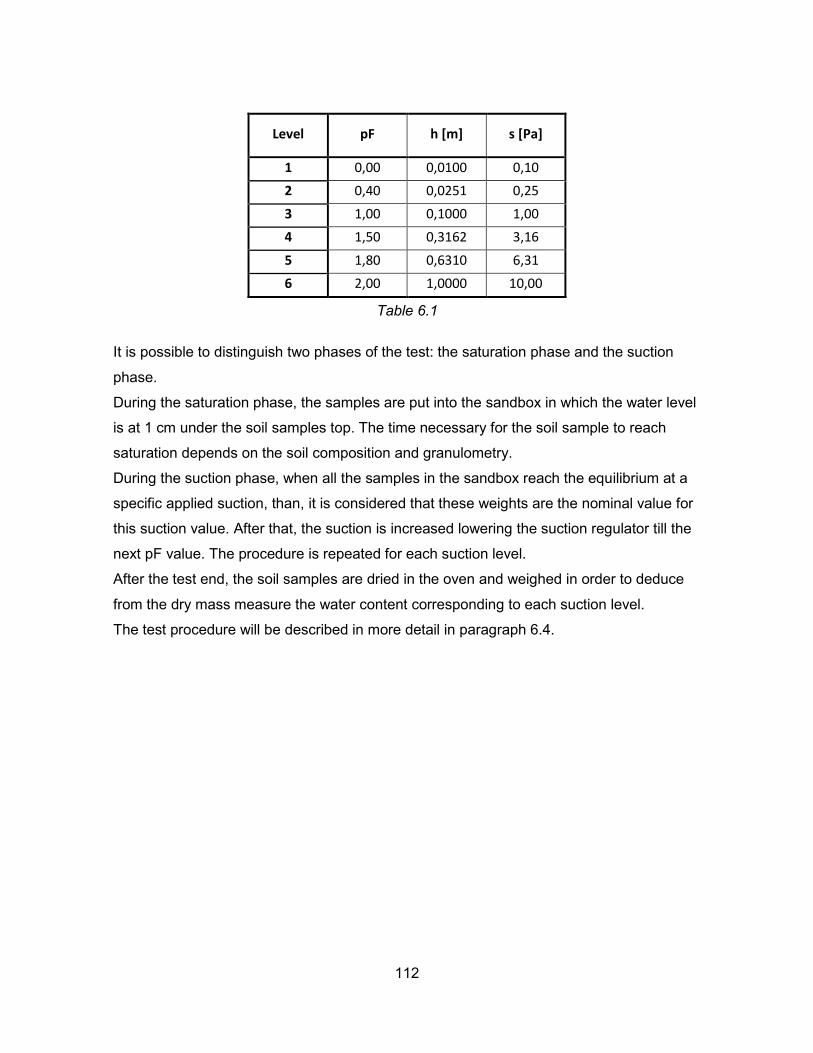
112
Level pF h [m] s [Pa]
1 0,00 0,0100 0,10
2 0,40 0,0251 0,25
3 1,00 0,1000 1,00
4 1,50 0,3162 3,16
5 1,80 0,6310 6,31
6 2,00 1,0000 10,00
Table 6.1
It is possible to distinguish two phases of the test: the saturation phase and the suction
phase.
During the saturation phase, the samples are put into the sandbox in which the water level
is at 1 cm under the soil samples top. The time necessary for the soil sample to reach
saturation depends on the soil composition and granulometry.
During the suction phase, when all the samples in the sandbox reach the equilibrium at a
specific applied suction, than, it is considered that these weights are the nominal value for
this suction value. After that, the suction is increased lowering the suction regulator till the
next pF value. The procedure is repeated for each suction level.
After the test end, the soil samples are dried in the oven and weighed in order to deduce
from the dry mass measure the water content corresponding to each suction level.
The test procedure will be described in more detail in paragraph 6.4.

113
6.2 PREPARATION OF THE SAMPLES
A typical sample used for the hanging column test is shown in figure 6.3 and figure 6.4.
It is composed by the following parts:
The soil sample compacted with the Proctor procedure.
A metal ring used to retrieve the sample from the Proctor mould.
A filter used to prevent the loss of material from the sample during the suction
experiment and the direct contact between the soil and the sandbox.
A string used to keep in tension the filter and to prevent it from moving.
Figure 6.3
Figure 6.4
The hanging column test was performed at the same time on the following 15 samples:
2 samples of T12;
2 samples of T12 5%;
2 samples of T12 7%;
2 samples of T12 12%;
2 samples of T3;
1 samples of T3 5%;
2 samples of T3 7%;
2 samples of T3 12%;
In figure 6.5 all the samples just before being put in the sandbox are shown.

114
Figure 6.5
Only one sample was made for the T3 5% due to the lack of a metal ring necessary for the
sample preparation. It has been chosen to sacrifice the T3 5% because the results of this
material are less important for the project of the CSM cap cover system. In fact, as
described in chapter 1, the CSM area is mainly formed by the T12 material while the T3
interests a smaller part of the site. Regarding the bentonite treatments, since in the final
cap cover system the use of the 7% one is previewed (chapter 4 paragraph 4.2.2), the
main concern is to show that T12 7% and T3 7% are characterised by an adequately low
hydraulic conductivity and that the 12% treatment does not decrease significantly this
value.
For the preparation of the samples the following procedure was followed:
1. Compaction of the untreated and treated soil with the Standard Proctor procedure.
2. Extraction of the sample from the Proctor mould with the normal compression
device.
3. Application of the filter and measure of the sample mass, height and volume.

115
The scale used for all the mass measures, made during the samples preparation, was
characterised by an accuracy of ±0,01 g.
6.2.1 Compaction with Proctor procedure
The first step in the preparation of the samples consists in compacting the soil and water
mixture with the Standard Proctor Procedure, already described in chapter 4.
Water was added to the mixture of soil and eventually bentonite in a quantitative equal to
wOPT+2%, where wOPT is the optimum water content found for the considered material with
the Standard Proctor test (chapter 4 paragraph 4.5).
After drying the material, it is possible to measure the effective water content of the
material compacted in the mould and the corresponding dry unit weight γd OPT+2%.
All the mentioned parameters are displayed for each material in table 6.2.
wOPT wOPT+2%
Calculated value wOPT+2%
Measured value d OPT+2% [kN/m3]
T12 0% 12,30% 14,30% 14,29% 18,77
T12 5% 14,90% 16,90% 17,91% 17,51
T12 7% 16,40% 18,40% 19,73% 16,92
T12 12% 17,60% 19,60% 21,36% 16,47
T3 0% 11,10% 13,10% 12,63% 19,46
T3 5% 14,20% 16,20% 16,77% 18,13
T3 7% 15,00% 17,00% 17,40% 17,95
T3 12% 15,20% 17,20% 18,38% 17,40
Table 6.2
It is possible to notice that, for almost all the materials, the actual water content is different
from the one calculated for the mixing. This happens due to inevitable imprecision
committed during the mixing (water not absorbed in a perfectly homogeneous way by the
soil, evaporation of water) and due to the initial water content of T12 and T3. In fact, the
actual water content values generally result slightly higher than expected. However, for the
purpose of the study, this does not represent a problem since, as mentioned in chapter 1
paragraph 1.4.3, soils used in cap cover systems are generally installed with a water
content equal to the optimum +2% or +3% and, in any case, included in the range
[wOPT+2%; wOPT+6%] (ADEME, BRGM, 2001).

116
From now on, the wOPT+2% expression will be used to refer to the measured value and not
to the calculated one to prepare the mixture.
6.2.2 Retrieving of the sample with normal compression
After the compaction, a metal ring was weighed and put on the surface of the compacted
soil in the Proctor mould. In order to make the metal ring penetrate into the soil, without
disturbing the sample, a normal compression device was used (figure 6.6). Moreover, a
lubrification by a thin layer of grease was applied on the metal ring surfaces before using
the normal compressor to make the punching easier.
Figure 6.6
The process is repeated another time using a second metal ring put on the opposite
surface of the soil in the mould.
The samples were obtained removing all the extra soil of the mould and eventually
levelling the surfaces of the sample to make them more homogeneous.
Therefore, from each mould prepared for a specific material, it was possible to obtain two
samples, which have been called E1 and E2. The only exception is the T3 5% for which
only the E1 has been prepared.

117
6.2.3 Measure of samples mass, height and volume
After putting the filters and the strings, the final samples have been obtained.
It is important to register the sample masses during their preparation in order to be able to
know the soil sample masses at every step. The following masses have been registered:
Metal ring mass (mring).
Soil and metal ring mass (msoil+ring).
Soil, metal ring, filter and string mass (msoil+ring)
Filter and string mass obtained from difference between msoil+ring+filter+string and
msoil+ring (mfilter+string).
These values, obtained at the end of each sample preparation, are displayed in table 6.3
and table 6.4 respectively for T12 and T3. The values are referred to a water content equal
to wOPT+2%.
T12 0% T12 0% T12 5% T12 5% T12 7% T12 7% T12 12% T12 12%
E1 E2 E1 E2 E1 E2 E1 E2
mring [g] 41,03 41,40 43,26 42,82 55,41 42,80 43,24 43,03
msoil+ring [g] 162,95 162,80 155,46 157,35 163,07 154,12 153,74 153,79
msoil+ring+filter+string [g] 164,78 163,95 157,30 159,09 164,90 155,99 155,55 155,66
mfilter+string [g] 1,83 1,15 1,84 1,74 1,83 1,87 1,81 1,87
Table 6.3
T3 0% T3 0% T3 5% T3 7% T3 7% T3 12% T3 12%
E1 E2 E1 E1 E2 E1 E2
mring [g] 42,39 41,92 43,55 41,35 42,77 43,25 41,80
msoil+ring [g] 162,03 166,84 159,23 158,20 156,57 157,87 158,13
msoil+ring+filter+string [g] 163,89 168,78 161,20 160,09 158,47 159,58 159,79
mfilter+string [g] 1,86 1,94 1,97 1,89 1,90 1,71 1,66
Table 6.4

118
Regarding the geometry of the samples, the height H was measured with the Vernier
calliper, the diameter D was constant for all the samples and the volume V was calculated
with the cylinder formula.
The values of D, H and V are indicated in table 6.5 and table 6.6 respectively for T12 and
T3.
T12 0% T12 0% T12 5% T12 5% T12 7% T12 7% T12 12% T12 12%
E1 E2 E1 E2 E1 E2 E1 E2
D [cm] 5,00 5,00 5,00 5,00 5,00 5,00 5,00 5,00
H [cm] 2,97 2,97 3,00 3,03 2,98 3,00 3,02 3,00
V [cm3] 58,32 58,32 58,90 59,49 58,51 58,90 59,30 58,90
Table 6.5
T3 0% T3 0% T3 5% T3 7% T3 7% T3 12% T3 12%
E1 E2 E1 E1 E2 E1 E2
D [cm] 5,00 5,00 5,00 5,00 5,00 5,00 5,00
H[cm] 2,96 3,01 3,03 2,99 2,98 3,00 3,03
V [cm3] 58,12 59,10 59,49 58,71 58,51 58,90 59,49
Table 6.6
6.3 PRELIMINARIES TO THE TEST
Before describing the test process (paragraph 6.4) it is necessary to introduce the
parameters and the equations used during the test to control its progress.
Moreover, since before concluding the test, samples dry masses are not accesible directly,
these values are in first approximation calculated from the Proctor test as explained in
paragraph 6.3.1. At the end of the test, after the drying in the oven, the true dry mass
values will be used for the parameters calculation (paragraph 6.5).
In paragraph 6.3.2 the equations used to calculate the water retention parameters are
shown.
Regarding the gravitational acceleration constant g and the water unit weight γw, the
following values were used:
Gravitational acceleration constant: g=10 m/s2.
Water unit weight: γw= 10 kN/m3.

119
6.3.1 Calculation of samples dry masses and dry unit weights
The dry masses of the samples are calculated with the following equation, which derives
directly from the definition of gravimetric water content (chapter 2 paragraph 2.1.1):
𝑚𝑑 =𝑚𝑠𝑜𝑖𝑙+𝑟𝑖𝑛𝑔 − 𝑚𝑟𝑖𝑛𝑔
1 + 𝑤 (6.3)
Where md is the dry mass (g) of the considered sample, msoil+ring and mring are the masses
(g) already defined in paragraph 6.2 and w is the gravimetric water content expressed in
decimal form.
The parameters of the equation 6.3 are assessed in reference to the Proctor procedure.
Therefore msoil+ring corresponds to the mass measured for the soil sample with the Proctor
mould and w corresponds to the wOPT+2% .
The values of msoil+ring and w have already been presented respectively in table 6.4 and
table 6.2 (paragraph 6.2).
The unit weights of the samples are calculated with the following equation:
𝛾𝑑 =𝑚𝑑
𝑉𝑔 (6.4)
Where γd is the unit weight of the considered sample (kN/m3), md is the dry mass of the
sample (kg), g is the gravitational acceleration (m/s2) and V is the volume of the sample
(m3) as calculated in paragraph 6.2.3 (table 6.5).
6.3.2 Calculation of water content parameters
In this paragraph, the equations used to calculate the gravimetric water content w, the
volumetric water content θ and the degree of saturation S are presented.
Gravimetric water content 𝑤 =𝑚𝑤
𝑚𝑑=
𝑚ℎ − 𝑚𝑑
𝑚𝑑 (6.5)
Where mw (g) is the water mass in the sample calculated as the difference between the
soil sample mass mh (g) and the dry sample mass md (g).
For measuring m attention must be paid in considering only the soil mass and not the
other elements forming the sample (metal ring, filter and string).
Volumetric water content 𝜃 = 𝑤 ∙𝛾𝑑
𝛾𝑤 (6.6)

120
Where γd is the dry soil unit weight (kN/m3) calculated with equation 6.4 and γw is the water
unit weight (kN/m3).
Degree of saturation 𝑆 = 𝑤 ∙𝛾𝑠𝛾𝑑
𝛾𝑤(𝛾𝑠 − 𝛾𝑑) (6.7)
Where γs is the unit weight of the solid fraction of the sample (kN/m3).
The equation 6.7 derives directly from the definition of degree of saturation (chapter 2
paragraph 2.2.1) in which the residual volumetric content was considered equal to zero.
The value of S must be between 0% (perfectly dry conditions) and 100% (saturation
conditions).
6.4 THE TEST PROCESS
In this paragraph, the running of the hanging column test will be described.
The test started the 22nd April 2014 and ended the 1st July 2014, for a total duration of 71
days.
In the following paragraphs, these aspects of the test process will be covered:
The test phases (preparation of the sandbox, saturation phase, suction phase).
Survey of temperature and humidity oscillations in the sandbox.
Problems encountered during the test.
The scale used for all the mass measures, made during the test, were characterised by an
accuracy of ±0,01 g.
6.4.1 Preparation of the sandbox
Before putting the samples in the sandbox, the instrumentation must be prepared for the
test. The detailed assembling of the sandbox is exposed in the Operating Instructions by
Eijkelkamp (2007), but in this work only the last steps of the preparation will be described
since the laboratory instrumentation had already been set for the utilization.
At first, the sand surface in the sandbox was smoothed and left to settle.
Then, the tap A (figure 6.2) was turned to the “supply” position and the tap B was opened
(figure 6.2) so that the water could flow from the supply bottle to the sandbox through the
sand drain removing the residual air bubbles.
Once about 1 cm of water level was reached above the sand, all the taps were closed.
Then, in order to remove possible bubbles entrapped between the sand and the protection

121
cloth, the surface was gently smoothed from the centre of the box to its sides.
After that, the tap A was turned to the “discharge” position to lower the water level to 0,5
cm above the sand surface. This 0,5 cm layer of water must be ensured in order to prevent
air to enter into the sand layer.
At the end of this process, all the taps were closed and all the prepared soil samples were
put in the sandbox with the bottom part, covered by the filter, in contact with the protection
cloth above the sand surface.
Before proceeding to the saturation phase and starting the test, it is fundamental to
prepare a map of the box so that the samples can be replaced to the exact position each
time they are taken out of the sandbox for measurements. Rotations of the samples in
relation to the original positions must be avoided too.
This procedure is important in order to be able to re-establish the same contact conditions
between the soil samples and the sandbox and, hence, to guarantee the same leakage
conditions during the test.
Figure 6.7 shows the samples in the sandbox and points out their positions.
Figure 6.7
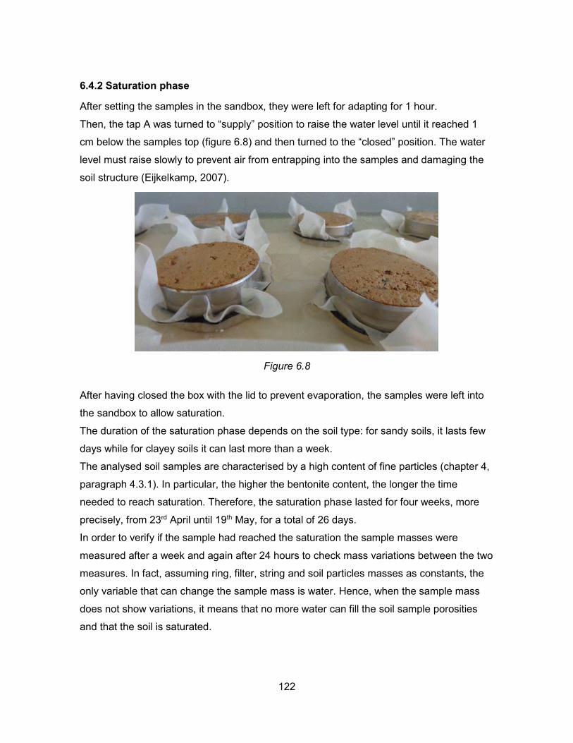
122
6.4.2 Saturation phase
After setting the samples in the sandbox, they were left for adapting for 1 hour.
Then, the tap A was turned to “supply” position to raise the water level until it reached 1
cm below the samples top (figure 6.8) and then turned to the “closed” position. The water
level must raise slowly to prevent air from entrapping into the samples and damaging the
soil structure (Eijkelkamp, 2007).
Figure 6.8
After having closed the box with the lid to prevent evaporation, the samples were left into
the sandbox to allow saturation.
The duration of the saturation phase depends on the soil type: for sandy soils, it lasts few
days while for clayey soils it can last more than a week.
The analysed soil samples are characterised by a high content of fine particles (chapter 4,
paragraph 4.3.1). In particular, the higher the bentonite content, the longer the time
needed to reach saturation. Therefore, the saturation phase lasted for four weeks, more
precisely, from 23rd April until 19th May, for a total of 26 days.
In order to verify if the sample had reached the saturation the sample masses were
measured after a week and again after 24 hours to check mass variations between the two
measures. In fact, assuming ring, filter, string and soil particles masses as constants, the
only variable that can change the sample mass is water. Hence, when the sample mass
does not show variations, it means that no more water can fill the soil sample porosities
and that the soil is saturated.

123
The registered weights are used to calculate water content at pF=0 (h=0,01 m) which,
hence, corresponds to the saturation conditions.
Due to the fluctuations in the samples masses measures, it was difficult to understand if
the samples had reached or not the saturation. Nevertheless, in order to avoid changing
the soil samples structure, saturation phase was concluded when a certain difference
between two consecutive mass measures of all the samples was reached.
The factors at the origin of these fluctuations in the measures will be described and
discussed in paragraph 6.5.
6.4.3 Suction phase
When all the samples contained in the sandbox were saturated, the suction phase was
started. It lasted from 19th May to 1st July for a total of 43 days.
During this phase tap A was maintained in “discharge” position and the suction regulator
was lowered to the following suction level each time that equilibrium was reached for all
the samples.
In order to define the equilibrium value of a sample, the sample was weighed two times
with an interval of 24 hours between the two measures. The water volumetric content θ
corresponding to the two measures was calculated with the equation 6.6. If the difference
between the two volumetric water contents was less than or equal to 0,20% the sample
was assumedin equilibrium. If this condition was not verified, the measures were repeated
at an interval of a week until the criterion was satisfied.
In some cases a difference in volumetric content slightly superior to 0,20% was accepted
because of the difficulty in reaching this limit value in reasonable times, especially for the
samples treated with 12% of bentonite. This choice was taken in order to avoid changes in
the soil samples structures.
Since the first level (pF=0,4) corresponds to a suction value near to the zero, sometimes
taking precise measures could be difficult. In our case the outflow water from the sandbox
was too small and the level lowering in the sandbox too slow. Therefore, since the pF=0,4
point corresponds to the situation in which the water level is equal to the sand level, the
suction regulator was temporarily lowered so that this situation could be reached.
After this first critical point, the standard procedure previously described was adopted.

124
6.4.4 Temperature and humidity survey
Since temperature variations affect water viscosity and hence water retention values, the
laboratory temperature should be constant between the measurements.
For verifying this condition, temperature and relative humidity in the sandbox were
monitored during the test with a temperature and humidity USB data logger. Thanks to this
system, temperature and humidity values can be monitored for long periods. Data have
been registered in the logger from 13th May to the 24th June each hour of the day.
After collecting the data in the computer, the graphic in figure 6.9 was obtained.
Figure 6.9
The average values are indicated with the dotted lines.
During the period of measure, the relative humidity was almost constant and near the
medium value of 105%. The temperature exhibited more variations, with peaks of ±5°C
respect to the medium value of 23,70°C. These variations were due to meteorological
changes and are still acceptable without alteration in the context of this test.

125
6.4.5 Dry samples masses and filters masses
When all the mass measurements of the samples were registered for each prefixed
suction level, the samples were removed from the sandbox, dried in the oven at 105°C and
weighted to obtain the true dry soil mass value md.
In order to correct the results the string mass mstring, the dry filter mass md (filter) and the
saturated filter mass msat (filter) were measured.
The dry filter masses were measured right after the drying in the oven.
The saturated filter masses were measured after immersing them in water.
In table 6.7 and table 6.8 the values of md, md (filter), msat (filter) and mstring are presented
respectively for T12 and T3.
T12 0% T12 0% T12 5% T12 5% T12 7% T12 7% T12 12% T12 12%
E1 E2 E1 E2 E1 E2 E1 E2
md [g] 105,77 104,54 93,45 96,33 88,20 91,81 89,46 89,79
md (filter) [g] 0,46 0,35 0,43 0,37 0,44 0,46 0,42 0,48
msat (filter) [g] 0,99 0,65 0,92 0,76 1,04 1,14 0,80 0,99
m (string) [g] 1,55 1,56 1,54 1,54 1,52 1,52 1,57 1,54
Table 6.7
T3 0% T3 0% T3 5% T3 7% T3 7% T3 12% T3 12%
E1 E2 E1 E1 E2 E1 E2
md [g] 104,70 109,18 98,07 97,65 95,56 94,85 96,99
md (filter) [g] 0,48 0,54 0,53 0,52 0,49 0,37 0,36
msat (filter) [g] 0,93 1,04 1,12 1,07 1,10 0,68 0,79
m (string) [g] 1,57 1,58 1,55 1,54 1,55 1,56 1,54
Table 6.8
6.5 PROBLEMS ENCOUNTERED AND CORRECTIONS
Interpretation and correction of results of the hanging column test is an important and
tricky phase. Actually, this test is subjected to a series of problems, which can affect
measures accuracy. Moreover, since the test is performed on small samples, even the
slightest change of the sample condition could affect dramatically the mass measurements
and, hence, the final results regarding the water retention.
Therefore, it was necessary to record all the possible reasons of discrepancy occurring

126
during the saturation and suction phase in order to correct the results.
In this paragraph, the following problems will be discussed:
Reference level for the zero suction,
Overestimation of the water content due to the water dripping from the filters,
Assessment of the filter mass during the experiment,
Swelling of the samples treated with bentonite,
Fine material loss from the samples,
Presence of mushrooms on the sample upper surface.
6.5.1 Reference level for the zero suction
As already mentioned, the reference level for zero suction is the middle of the soil sample,
but the free water level is 1 cm below the top of the sample. Therefore, the moisture
tension ranges from +1 cm at the bottom of the sample, to H-1 cm at the top of the sample,
where H is the sample height (Eijkelkamp, 2007).
This inaccuracy is intrinsic of the test saturation procedure and affects the precision of the
water content calculation at saturation (pF=0). Nevertheless, this imprecision becomes
less and less relevant with the suction increasing (Eijkelkamp, 2007).
6.5.2 Overestimation of water content
When the samples are taken out from the sandbox for the measurements, the change in
water content is inevitable (Eijkelkamp, 2007).
It was noticed that extra water dripping from the sample could influence the sample mass
measure leading to an overestimated water content.
In fact, calculating the degree of saturation S during the first phases of the test with the
equation 6.7, values superior to 100% were found. Nevertheless, as already stated in
paragraph 6.3.2, the maximum value of S is 100% at which the sample is saturated.
Hence, when values of S superior to 100% were found, this meant that the soil sample
water content was being overestimated.
In order to mitigate this effect to the minimum, the following procedure was adopted to
obtain the mass measures both during saturation and suction phase:
1. The sample was removed from the sandbox, letting the extra water drip directly into
the sandbox.

127
2. The sample was put on a plate to let further dripping of the extra water
3. The sample was put on the scales and the mass was recorded.
Different steps were carried out quickly in order to remove only extra water from the
sample and to avoid changing the soil sample water content.
This problem was more relevant for the untreated materials than for the treated ones. This
is probably due to the fact that the bentonite inside the treated samples helps the soil to
retain more water in the porosity.
Moreover this problem was mainly related to the saturation phase since the samples were
immersed in water. In fact, with the increasing suction and the subsequent lowering of the
water level into the sandbox, the presence of extra water became less and less actual. In
fact, on the plate used in the second step of the procedure we could find less and less
water proceeding with the test.
6.5.3 Assessment of filter mass during the experiment
In order to obtain the gravimetric water content through the equation 6.5, it was necessary
to calculate the humid soil mass removing from the recorded sample, the contribution of
the string, the metal ring and the filters.
While the string mass and the metal ring mass do not depend on the presence of water
and remain constant during all the experimentation, the filter masses depend on the kept
of the water. The masses of the dry and saturated filters were recorded as explained in
paragraph 6.4.5 but it is not possible to know the variation of the filter masses during the
test.
In this study, it was decided to use always the saturated filter mass value for calculating
the gravimetric water content with the equation 6.5. In fact, it was assumed that the filters
are characterised by the ability to retain water even during the suction phase (porous
medium with a high air entry pressure).
Therefore, the water mass inside each sample, mw, was calculated with the following
equation:
𝑚𝑤 = 𝑚ℎ − 𝑚𝑑 − 𝑚𝑟𝑖𝑛𝑔 − 𝑚𝑠𝑡𝑟𝑖𝑛𝑔 − 𝑚𝑠𝑎𝑡 (𝑓𝑖𝑙𝑡𝑒𝑟) (6.8)
Where mh is the humid mass of the sample measured during the saturation or suction
phase (g), md is the dry mass of the soil sample (g), mring is the metal ring mass (g), mstring
is the plastic string mass (g) and msat (filter) is the mass of the saturated filter (g).

128
mring values have been presented in paragraph 6.2.3.
md, mstring and msat (filter) values have been presented in paragraph 6.4.5.
6.5.4 Swelling of the samples
During the saturation phase, all the treated samples exhibited swelling.
Because of the high content in bentonite, the first samples to swell under a given suction
were the T12 12% and T3 12%, followed by T12 7% and T3 7% and finally by T12 5% and
T3 5%.
When swelling occurs, the soil sample volumes as calculated in paragraph 6.2.3, are not
any more constant during the test. In order to determine the correct gravimetric water
content w (equation 6.5) and consequently the volumetric water content θ (equation 6.6)
and the degree of saturation S (equation 6.7), it was necessary to recalculate the volume
each time the sample mass had to be registered.
Because of the metal ring confining the sample laterally, the diameter remained constant
even with the swelling. Hence, the parameter changing with the swelling was the sample
height.
Each time the sample masses had to be recorded, the following procedure was followed
for the samples exhibiting swelling:
1. The height was measured with a Vernier calliper.
2. The measure was repeated three times for each sample.
3. The final sample height was calculated as the arithmetic mean of the three
measured values.
4. The new volume was calculated with the cylinder formula.
5. The new dry unit weight of the swelled samples was calculated with the equation
6.4.
6. The gravimetric water content w, the volumetric water content θ and the degree of
saturation S were calculated respectively with the equation 6.5, equation 6.6 and
equation 6.7.
During the operations with the Vernier calliper, attention was paid to avoid disturbing the
sample and removing soil from its surface in order not to change the mass.
Looking at the heights measurements (attachment), it is possible to notice that heights
increased due to the swelling but began decreasing after a certain point. It means that the

129
soil samples were subjected to shrinkage in the last part of the test.
The first samples to shrink were the T12 12% and T3 12%, followed by the samples
containing less bentonite, hence, the T12 7% and T3 7% and finally the T12 5% and T3
5%.
The swelling of T12 12% and T3 12% was monitored during all the experiment since these
samples exhibited swelling at the beginning of the saturation phase. The swelling of T12
5%, T12 7%, T3 5% and T3 7% started to be observed during the suction phase because
the swelling occurring during the saturation phase was not well visible.
Nevertheless, the first measurements of swelling of T12 5%, T12 7%, T3 5% and T3 7%
were extended to the beginning of the suction phase in order to homogenise the results
and obtain more realistic SWRCs.
6.5.5 Fine material loss from the samples
During the suction phase, the samples exhibited a loss of the finer material that could
affect the results. However, the soil particles loss was particularly relevant for the
untreated samples, T12 and T3 as shown in figure 6.10.
Figure 6.10
This issue will be discussed more in detail in chapter 7 in order to analyse the erosion
susceptibility of the samples and the influence of the bentonite treatments on this matter.

130
6.5.6 Presence of mushrooms on the sample upper surface
During the saturation phase, some mushrooms appeared on the upper surface of the
samples due to biological activity facilitated by the humid conditions in the sandbox.
In figure 6.11 the surface of a sample attacked by the mushrooms is displayed.
These mushrooms could change the soil properties if free growing was allowed.
In order to overcome this problem a disinfectant solution with a 2,5% concentration of
glutarldehyde was used. The solution was distilled directly on the surface of the infected
samples. This operation had to be done always after the mass measurements in order not
to add extra weight on the samples.
This treatment was repeated three times during the experiment and was sufficient to
overcome this problem.
Figure 6.11
6.5.7 Calculation of the degree of saturation S
During the saturation phase and the beginning of suction phase (pF=0,4) the calculated
value of S was superior to 100%, hence, since this is physically not possible, it was
affected by a series of systematic errors.
Assuming that the measures of the metal ring diameters D and of the solid unit weights γs
are sufficiently accurate, errors were mainly due to the following imprecisions:
All the taken mass measures the soil sample dry mass md an error of measure of
±m is committed. The real masses are equal to m±m.

131
Measuring the height H of samples exhibiting swelling an error of measure of ±H
is committed. The real height is equal to H±H.
Therefore, these inaccuracies affect the determination of the soil sample volume V, the dry
unit weight γd (equation 6.4), the gravimetric water content w (equation 6.5), the volumetric
water content θ (equation 6.6) and the degree of saturation S (equation 6.7).
In particular, since S is calculated using w and γd, equation 6.7 tends to increase the error
amount of the calculation.
Figure 6.12 helps to clarify the impact of these errors on S.
Figure 6.12
In light of these considerations, in order to calculate S its definition, already presented in
chapter 2 paragraph 2.1.1, was used instead of equation 6.7. The S definition is reported
underneath:
𝑆 =𝜃 − 𝜃𝑟
𝜃𝑠𝑎𝑡 − 𝜃𝑟 (6.10)

132
As already stated in paragraph 6.3.2 the residual volumetric water content was set equal
to zero for all the studied samples. Equation 6.10 has the advantage of depending directly
on the volumetric content θ.
θ corresponds to the porosity fraction of the sample completely filled by water. When the
soil sample is completely saturated, water fills all its porosities. Hence, the volumetric
water content corresponding to the saturation conditions θsat can be set equal to the
porosity n of the sample.
Nevertheless, considering the treated samples, the porosity n was not constant during the
experiment because of the swelling and the shrinkage. Hence, at the end of the test, for
each sample, the maximum volumetric water content θmax, calculated with the equation
6.6, was imposed to correspond to saturation conditions and, hence, to be equal to θsat.
In light of these considerations, the equation 6.10 can be written as following:
𝑆 =𝜃
𝜃𝑚𝑎𝑥=
𝜃
𝑛 (6.11)
In table 6.9 and table 6.10 the maximum volumetric water content calculated during the
experiment are presented and it is assumed that the θmax, corresponds to the porosity n,
are respectively for T12 and T3.
T12 0% T12 0% T12 5% T12 5% T12 7% T12 7% T12 12% T12 12%
E1 E2 E1 E2 E1 E2 E1 E2
θmax = n 0,3702 0,3555 0,4203 0,4189 0,4444 0,4312 0,5181 0,4906
Table 6.9
T3 0% T3 0% T3 5% T3 7% T3 7% T3 12% T3 12%
E1 E2 E1 E1 E2 E1 E2
θmax = n 0,3821 0,3606 0,4116 0,4558 0,4360 0,5386 0,5224
Table 6.10
It is possible to notice that the maximum values generally do not happen to be at pF=0 but
towards the end of the saturation phase for the untreated samples, or at pF=0,4 for the
treated ones. This means that the corresponding S values calculated with the equation
6.11 are not equal to 100% at pF=0.
In order to be able to apply the Van Genuchten model (paragraph 6.6), the S values at

133
pF=0 were fixed to 100%.
The final values of S obtained from the test are shown in the attachment.
In table 6.11 the equations already described in the previous paragraphs and to calculate
S from the experimental data are displayed. The meaning of all the parameters appearing
in the equations have already been explained in the previous paragraphs.
Water mass 𝑚𝑤 = 𝑚ℎ − 𝑚𝑑 − 𝑚𝑟𝑖𝑛𝑔 − 𝑚𝑠𝑡𝑟𝑖𝑛𝑔 − 𝑚𝑠𝑎𝑡 (𝑓𝑖𝑙𝑡𝑒𝑟) [g]
Dry unit weight 𝛾𝑑 =𝑚𝑑
𝑉𝑔 [kN/m3]
Gravimetric water
content 𝑤 =
𝑚𝑤
𝑚𝑑 %
Volumetric water
content 𝜃 = 𝑤 ∙
𝛾𝑑
𝛾𝑤 %
Porosity 𝑛 = 𝜃𝑚𝑎𝑥 = 𝜃𝑠𝑎𝑡 adimensional
Degree of
saturation 𝑆 =
𝜃
𝜃𝑚𝑎𝑥 %
Table 6.11
6.6 APPLICATION OF THE VAN GENUCHTEN MODEL
In this paragraph, the data obtained for the degree of saturation S will be used to build the
Van Genuchten model.
From this point forward, the subscripts EXP and VG will be used to indicate, respectively,
a curve referred to the experimental values and a curve referred to the Van Genuchten
model.
It is necessary to found the parameters of the Van Genuchten model in order to make
some considerations on how the hydraulic conductivity of the studied samples changes
when the soil is in partially saturated conditions.
In this study, since the data were obtained using only the hanging column test data the
curves describe the soil retention properties referring only to the structural porosity of the
samples. In fact, the suction values applicable with the hanging column test are not low
enough to remove the water filling the microporosities of the samples.

134
6.6.1 The experimental Soil Water Retention Curve
In figure 6.13 and figure 6.14 the h(S)EXP respectively for T12 and T3 are shown. The data
used to plot these curves are shown in the attachment.
Figure 6.13

135
Figure 6.14
These curves show the suction h expressed in water column, in function of the degree of
saturation S, calculated as described in paragraph 6.5.7.
Considering the two graphics, it is not easy to discuss the effect of bentonite treatments
since there is not a clear tendency in the disposition of the curves. This is probably due to
the problems encountered during the experiment and already discussed in paragraph
6.5.7.
Therefore, the curves h(S)EXP will be used only to find the parameters of the Van
Genuchten model.
In order to comment the effect of the bentonite treatments on the raw soils, the curves h(θ)
were used instead of the h(S). These curves will be discussed in paragraph 6.7.2.
6.6.2 The Van Genuchten model parameters
The Van Genuchten model was already described in chapter 2, paragraph 2.3.3. The
equations are reported underneath:

136
𝑆 = (1
1 + (𝛼 ∙ ℎ)𝑛)
𝑚
(6.12)
𝑚 = 1 −1
𝑛 (0 < 𝑚 < 1) (6.13)
Where the meaning of the parameters is the same already explained in chapter 2
paragraph 2.3.3.
In order to build the model, it is necessary to estimate the values of α, m and n.
Nevertheless, since m and n are correlated with equation 6.13, equation 6.12 can be
written with the following expression:
𝑆 = (1
1 + (𝛼 ∙ ℎ)1
1−𝑚
)
𝑚
(6.14)
Therefore, it is sufficient to estimate the value of the two parameters: α and m.
For doing so, the Scilab program reported in the attachment was implemented for each
soil sample used in the hanging column test.
Chosen the sample to analyse, the program aim is to find a couple (α,m) for which the
variance between the experimental values of the saturation degree and the corresponding
model values is minimal. In order to realize this objective, the following function was
defined:
𝑅𝑀𝑆 =
√∑ (𝑆𝑘 𝐸𝑋𝑃 − 𝑆𝑘 𝑉𝐺)2𝑁𝑘=1
𝑁
(6.15)
Where k is the index corresponding to an equilibrium point in the curve and N is the total
number of equilibrium points of the experimental curve, hence, N=5 in this study.
Summarizing, the program uses the following procedure for each soil sample:
1. The parameters used in the program are defined.
2. The input data, that are the values of suction h and of saturation degree SEXP, are
defined.
3. The number of test couples (α,m) is chosen.
4. The values of αi and mi for the i-th test couple are randomly chosen by the program
in the interval [0;1].

137
5. For each k-th suction value h, the program calculates the Si VG with the equation
6.14.
6. For each i-th test couple, the program calculates the RMS with the equation 6.15.
7. Steps from 4 to 6 are repeated for all the test couples (cfr. Step 3).
8. The program extrapolates the (α,m) values corresponding to the minimum RMS
and calculates the n value with the equation 6.13.
Since the couple (α,m) is chosen randomly by the program, the model reliability strictly
depends on the number of test couples chosen at point 3: the higher this number, the
more reliable the model. Thanks to the Scilab program, it was possible to test 1000000 of
couples for each sample. After, in order to check the model reliability, it was checked that
already with 100000 couples, the minimum values of RMS were negligibly higher than the
ones obtained with 1000000 couples.
In table 6.12 and table 6.13 the gained values of α, m and n are displayed respectively for
T12 and T3 samples.
T12 0% T12 0% T12 5% T12 5% T12 7% T12 7% T12 12% T12 12%
E1 E2 E1 E2 E1 E2 E1 E2
α [cm-1] 0,64408 0,68817 0,56654 0,57217 0,63934 0,63569 0,55224 0,52495
n 1,03304 1,02839 1,03562 1,03385 1,04475 1,03657 1,02622 1,02481
m 0,03199 0,02761 0,03439 0,03275 0,04284 0,03528 0,02555 0,02421
RMS 0,01671 0,01410 0,02154 0,02078 0,02979 0,02425 0,01562 0,01428
Table 6.12
T3 0% T3 0% T3 5% T3 7% T3 7% T3 12% T3 12%
E1 E2 E1 E1 E2 E1 E2
α [cm-1] 0,54837 0,47148 0,52909 0,49910 0,62907 0,54670 0,46845
n 1,06387 1,04517 1,04202 1,05179 1,04171 1,03839 1,03793
m 0,06004 0,04322 0,04033 0,04924 0,04004 0,03697 0,03654
RMS 0,03332 0,02264 0,02365 0,02743 0,02737 0,02271 0,01936
Table 6.13
6.7 RESULTS
In this paragraph, the data collected thanks to the hanging column test will be elaborated
and discussed.
138
As already disclosed in paragraph 6.6.1, since the calculation of the degree of saturation
was problematic (paragraph 6.5.7), the curves h(S) were not used to comment the effect of
the bentonite treatments. Therefore, in order to draw some conclusions concerning the
bentonite treatments of T12 and T3, h(θ) and γd(θ) curves were used.
The volumetric water content was chosen as a reference since it is less influenced than
the degree of saturation by the variations of the sample volumes as already explained in
paragraph 6.5.7. The intent of this approach was to study separately the variations of the
samples water contents, and the effects of swelling and shrinkage on the treated samples.
In fact, from the comparison between the 6.6 (θ) and the 6.10 (S), it is possible to notice
that the influence of swelling and shrinkage lies only in the γd value for the calculation of θ,
and both in θ and in the θmax value for the calculation of S.
In paragraph 6.7.1, the solid unit weight γs will be estimated and compared to the ones
resulting from the water pycnometer test (Chapter 4 paragraph 4.4).
In paragraph 6.7.2 the h(θ) will be presented to discuss the relation between these curves
and the retention properties of the samples.
In paragraph 6.7.3 the γd(θ) will be presented to study the effect of swelling and shrinkage.
Finally in paragraph 6.7.4, the hydraulic conductivity of the samples will be extrapolated
thanks to the Van Genuchten model.
6.7.1 Estimation of the solid unit weight
The solid unit weight γs was determined with the pycnometer method as explained in
chapter 4 paragraph 4.4. However, in order to calculate the degree of saturation S these
values were not used since the equation 6.10 was used.
In this paragraph, the solid unit weight of the hanging column test will be compared to the
values obtained from the pycnometer method in order to make some considerations on the
reliability of the test results.
The solid unit weight calculated from the test will be called γs (test) while the one obtained
from the pycnometer method will be called γs (pyc).
γs (test) was calculated from the definition of solid unit weight:
𝛾𝑠 =𝑚𝑠
𝑉𝑠∙ 𝑔 (6.16)

139
Where γs is the solid unit weight (kN/m3), ms is the solid mass (kg), Vs is the volume
occupied by the solid mass (m3) and g is the gravitational acceleration (m/s2).
The solid mass ms is equal to the samples dry mass md (paragraph 6.4.5) while Vs is
calculated with the following expression:
𝑉𝑠 = 𝑉 − 𝑛 ∙ 𝑉 (6.17)
Where V is the sample volume (m3) and n is the sample porosity (adimensional).
Therefore, γs (test) was calculated with the following equation obtained from the equation
6.16 and the equation 6.17:
𝛾𝑠 (𝑡𝑒𝑠𝑡) =𝑚𝑑
𝑉 ∙ (1 − 𝑛)∙ 𝑔 (6.18)
Due to swelling and shrinkage, V and n are not constant. For the assessment of γs (test) the
saturation condition was chosen as a reference and, hence, the values of V and n
corresponding to S=100% were considered.
The error of γs (test) was calculated in percentage with the following expression:
𝐸 [%] =𝛾𝑠 (𝑡𝑒𝑠𝑡) − 𝛾𝑠 (𝑝𝑦𝑐)
𝛾𝑠 (𝑝𝑦𝑐) (6.19)
In table 6.14 and table 6.15 the values of γs (test), γs (pyc) and E are displayed respectively for
T12 and T3.
T12 0% T12 0% T12 5% T12 5% T12 7% T12 7% T12 12% T12 12%
E1 E2 E1 E2 E1 E2 E1 E2
γs (test) [kN/m3] 28,80 28,80 28,51 28,23 28,70 28,51 28,32 28,51
γs( pyc) [kN/m3] 26,79 26,79 26,77 26,77 26,76 26,76 26,74 26,74
E 7,49% 7,49% 6,50% 5,44% 7,25% 6,53% 5,90% 6,61%
Table 6.14
T3 0% T3 0% T3 5% T3 7% T3 7% T3 12% T3 12%
E1 E2 E1 E1 E2 E1 E2
γs (test) [kN/m3] 28,90 28,42 28,23 28,61 28,70 28,51 28,23
γs( pyc) [kN/m3] 27,36 27,36 27,31 27,29 27,29 27,25 27,25
E 5,61% 3,85% 3,36% 4,81% 5,17% 4,63% 3,60%
Table 6.15

140
It is possible to notice that the γs (test) is always higher than the real solid unit weight γs(pyc).
For how it has been calculated, E represents the error committed for the evaluation of γs.
The value of E does not depend on the treatment since it is not possible to find any
particular tendency in function of the bentonite percentage.
The error is higher for the T12 but, in any case, it is always under the 8% for all the
samples studied with the test. Hence, it is possible to conclude that the problems
encountered during the saturation phase have not invalidated the test results.
6.7.2 Soil Water Retention Curves
For the reasons already explained in the introduction of paragraph 6.7, the SWRC of the
samples were finally traced referring to the volumetric water content.
In figure 6.15 and figure 6.16, respectively, the h(θ) curves of T12 and T3 and their
treatments are displayed. The graphics show both the experimental points obtained with
the hanging column test and the curves obtained with the Van Genuchten model.
The model underestimates the initial θ (pF 0 and pF 0,4 – saturation conditions) and the
last two points (pF 1,8 and pF 2) and overestimate the central points (pF 1 and pF 1,5).
Underestimations and overestimations are mainly due to the lack of a consistent number
of points ranging from saturation conditions (zero suction) to very dry conditions (high
suction values).
In fact, the Van Genuchten model was thought to describe the complete SWRC but, with
the hanging column test, it is possible to study only its first part corresponding to low
suctions. Nevertheless, the adaptation of the curve can be considered enough precise for
the purpose of this work.

141
Figure 6.15
Figure 6.16

142
It is possible to observe that, increasing the bentonite content, the samples are able to
retain more water. In fact, the volumetric water content of a sample with a higher bentonite
rate is always higher than a sample containing less bentonite. This observation is valid, for
both T12 and T3, at saturation and during the entire suction phase.
Therefore, the higher the bentonite content, the higher the water content that the sample is
able to retain.
6.7.3 Observations on swelling and shrinkage
As already exposed in paragraph 6.5.4 the samples exhibited swelling during the initial
phases of the test and shrinkage in the ending phase. In order to study these phenomena
the γd(θ) curves have been traced.
In this paragraph, only the γd(θ) curves for T12 12% and T3 12% will be shown because
the effects of swelling and shrinkage are more evident. Nevertheless the observations that
will be made for these samples remain valid for the T12 5%, T12 7%, T3 5% and T3 7%.
Figure 6.17

143
Figure 6.18
In figure 6.17 and figure 6.18 the γd(θ) curves of T12 12% and T3 12% respectively are
exposed. In the graphics θ increases from left to right in the x axis, hence, considering the
hanging column test procedure, the suction increases from right to left. The labels next to
the points indicate the corresponding suction level in pF value. The dotted lines indicate
the dry unit weight values of the samples at the beginning of the test.
Since swelling and shrinkage change the samples volumes, they affect the calculation of
the dry unit weight γd (equation 6.4).
In particular, γd changes in the following manner:
Swelling V increases γd decreases.
Shrinkage V decreases γd increases.

144
This behaviour is confirmed by the graphics.
It is possible to notice that there is a consistent decrease of the dry unit weight from the
initial values (Proctor unit weights referred to the sample).
Moreover, it is possible to outline another aspect observing the last three points of suction
(pF=1; pF=1,5; pF=2). These three points belong to the shrinkage phase and tend to
distribute along a vertical line. This means that in the suction interval pF=[1 – 2], γd
increases while θ remains almost constant.
This aspect is schematised in figure 6.19, where, considering a volume unit of the sample,
A represents a suction equilibrium point in the interval pF=[1 – 2] and B the successive
equilibrium point in the same interval.
Figure 6.19
The unit volume consists of a triphasic system (gas, solid and water). The water phase can
be considered constant in the passage from A to B due to the observation made
previously. Since the mass contribute of the gas phase is not significant, the increase of
the dry unit weight is due to an increment in the solid phase to the detriment of the
gaseous phase. Therefore, when the sample passes from A to B, the soil particles are
attracted into the triphasic unit volume with a consequent decrease of the sample porosity.

145
6.7.4 Estimation of the hydraulic conductivity
In this paragraph, the evolution of the hydraulic conductivity with the suction will be
presented.
The values of hydraulic conductivity can be extrapolated from the hanging column test
results thanks to the Van Genuchten model which provides a relation between the relative
hydraulic conductivity Kr and the saturation degree S. The relation have been already
discussed in chapter 2 paragraph 2.3.3, and it is reported underneath:
𝐾𝑟 =𝐾(𝑆)
𝐾𝑠𝑎𝑡= 𝑆1/2[1 − (1 − 𝑆1/𝑚)
𝑚]
2 (6.20)
Where K(S) is the hydraulic conductivity corresponding to a certain degree of saturation
(m/s), Ksat is the saturated hydraulic conductivity (m/s) and m is the Van Genuchten
parameter as calculated for each sample (paragraph 6.6.2).
In the equation 6.20, the experimental values of the degree of saturation, Sexp, were
considered because the ones provided by the Van Genuchten model, SVG, are less
realistic. In fact, the use of SVG would give back very low values of Kr and, in particular the
first point at saturation (pF 0) would not correspond to Kr=1 because the model, as already
observed in paragraph 6.7.2, does not give back S=100% at the zero suction (pF 0).
After having obtained the values of Kr, they were traced in function of the measured
volumetric water content θ.
The Kr(θ) curves are shown in figure 6.20 and figure 6.21 respectively for T12 and T3.

146
Figure 6.20
Figure 6.21

147
Thanks to these graphics it is possible to comment the effect of the bentonite treatments
on the raw material in slightly unsaturated conditions.
The rate at which the relative hydraulic conductivity Kr of the materials changes with the
volumetric water content θ slightly increases with the increase of bentonite content.
It is possible to observe that some of the samples can reach lower values of Kr for the
same suction level. In order to comment this aspect the h(K) curves were traced. The
hydraulic conductivity K was calculated for each sample at each suction level using the
definition of Kr (equation 6.20), in which the value of Ksat is the one obtained with the oedo-
permeameter (chapter 5 paragraph 5.1.3). In fact, this test was repeated multiple times for
each sample and, hence, its results can be considered reliable.
In figure 6.22 and figure 6.23, h(K) curves are presented respectively for T12 and T3.
Figure 6.22

148
Figure 6.23
In the graphics, the K value corresponding to zero suction (pF 0) is the hydraulic
conductivity measured in saturated conditions (Ksat).
In saturated conditions, the higher the bentonite content, the lower the measured Ksat but
the efficiency of the treatment reaches its maximum with the 7% of bentonite, among the
studied percentages. In fact, increasing the bentonite percentage from 7% to 12% does
not improve significantly the impermeability of the material.
Regarding the suction phase, the same considerations are valid.
Moreover, it is possible to observe that the higher the suction level, the lower the hydraulic
conductivity K. This effect is evident for the raw materials but becomes less visible
increasing the bentonite content of the material. In fact, observing figure 6.22 and figure
6.23, it is possible to see that the h(K) curves of T12 7%, T12 12%, T3 7% and T3 12%
tend to assume the shape of a vertical line.
This behaviour depends on the fact that the samples containing more bentonite are able to
retain more water, as already seen in paragraph 6.7.2, and that the suction applied with

149
the hanging column test is not sufficiently high to see a significant change in the hydraulic
conductivity from the saturated value obtained with the permeameter.
6.8 CONCLUSIONS ON THE HANGING COLUMN TEST
The conclusions drawn for the hanging column test will be presented and summarised in
this paragraph.
The treated samples exhibited swelling during the saturation phase and shrinkage
in the last part of the suction phase. These phenomena did not take place during
the oedometric tests in which the samples were more confined.
The volume variations of the treated soil due to the water content should be
considered for the project of the final cap cover system of the CSM, in
consideration of the confinement in situ of the cap cover.
Considering equal suction conditions, the higher the bentonite content of the
analysed material, the higher the water content.
Increasing suction, the hydraulic conductivity of all the samples decreases but the
effect is more evident for the raw materials than for the treated samples.
In the final part of the suction phase pF=[1,2] of the treated samples, the dry unit
weight lowers while the water content remains constant.
This aspect may be relevant for the CSM project. In fact, the future cap cover
system could exhibit a variance of the dry unit weight when slightly under
saturation S=[80%, 90%].
The raw material (T12 and T3) tend to lose the fine particles during the test.
Increasing the bentonite content this phenomenon becomes less and less relevant.
This issue will be analysed in chapter 7.
The considerations presented above are valid in the field studied with the hanging column
test and, hence, in the suction interval pF=[0,2] corresponding, for the analysed soils, to a
degree of saturation approximatively in the interval S=[80%,100%].
Since the suction applicable with the hanging column test are limited, it was possible to
remove only the water filling the structural pores of the soil samples.
For further studies on the effect of bentonite treatments in unsaturated conditions other
tests, able to reach higher suction values, should be performed.

150

151
CHAPTER 7 Soils sensitivity to erosion
In this chapter, the sensitivity to erosion of T12 and T3 is analysed.
The urge to analyse this matter and to intend to explain the erosion process is due to the
loss of fine particles shown by the T3 in the permeameter test (chapter 5) and in the
hanging column test (chapter 6).
After describing the problem (paragraph 7.1), the internal stability of the untreated
materials will be analysed in paragraph 7.3 referring to the complete granulometric curve
(T12 and T3) and the 0/5 mm fraction (T120/5 and T30/5).
Since the results of the internal stability criteria will show that there is not much difference
in considering the complete granulometric curve and the 0/5mm fraction, the external
erosion criteria will be applied only to the 0/5mm fraction (paragraph 7.4).
Moreover, the external erosion criteria based on Atterberg limits will be applied to analyse
the effect of bentonite treatments on the sensitivity to erosion of T12 and T3.
7.1 PRESENTATION OF THE PROBLEM
In chapter 5 and chapter 6 the oedo-permeameter test and the hanging column test,
respectively, were described. For both the test soil particles loss from the tested samples
was observed.
Regarding the permeameter test, the deposit of fine soil in the outflow pipe indicated that
the water outflowing from the sample contained fine particles. This tendency was
particularly obvious for T3.
T12 and T3 exhibited the same tendency in the hanging column test. In fact, the untreated
samples, in particular T3 more than T12, lost the fine particles leaving in the sandbox a
coloured circle of material as shown in figure 7.1.

152
Figure 7.1
Figure 7.2
Moreover, thanks to the hanging column test, it was possible to find out that also the
treated samples suffer a loss of finer material but with a minor rate as the bentonite
content increases. This behaviour is clearly presented in figure 7.2, showing the filter put
at the base of every sample above the sandbox, after having removed all the samples at
the end of the test.
Figure 7.3

153
The tests conditions are summarised underneath.
The oedo-permeameter test was performed under the following conditions:
The tested samples have been realised from the 0/5 mm fraction of the
granulometric curve;
The laboratory temperature is kept around 20°C;
The tested samples have been compacted with the Proctor procedure using
different water contents but always equal or slightly superior to the optimum
content (wOPT);
A low confinement of 26 kPa corresponding to a layer of soil a little bit thicker than
1m;
The applied hydraulic charge is of 10 cm.
The hanging column test was performed under the following conditions:
The tested samples have been realised from the 0/5 mm fraction of the
granulometric curve;
The sandbox temperature is constantly measured to verify that it remains around
20°C;
The tested samples have been compacted with the Proctor procedure using a
water content equal to wOPT+2%;
The samples have been obtained using metal rings (diameter = 5 cm, height ≈ 3
cm);
The samples are separated from the kaolinitic sand of the sandbox by a filter
directly put on the sand and by a filter put on each sample;
The samples are dried increasing the suction value to the next one and waiting for
the stabilisation until all the samples reach the equilibrium, hence, when the
difference in the volumetric water content θ between two measures of two
consecutive days is approximately less than 0,2%.
7.1.1 Possible impact on the behaviour of the landfill soil cover
The loss of material could be a problem for the cover system since the phenomenon of
erosion may affect negatively the mechanical resistance and the impermeability of the

154
system.
In general, it is possible to distinguish two kinds of possible causes of erosion depending
on whether it has an impact on the mechanical resistance or on the impermeability of the
structure (Pham, 2008).
A low mechanical resistance may be due to:
Poor compaction;
Absence of a proper filter;
Use of dispersive materials ( clay, silt, fine sand).
An increase of permeability may be due to:
Bad choice of the materials;
Presence of cracks.
Even if the causes of low mechanical resistance and bad impermeability were presented
separately, in reality the two conditions are interdependent.
In order to analyse the tendency of the two soils to lose material the internal stability,
geometric criteria (paragraph 7.3) and external erosion criteria (paragraph 7.4) will be
applied.
7.2 INTERNAL AND EXTERNAL EROSION
When a soil is subjected to water flow, its smaller particles may be removed by the flux of
water causing a rearrangement of the soil structure.
According to how this phenomenon takes place, different terms have been introduced
leading sometimes to confusion in literature to describe the process. In this paragraph, this
issue will be clarified distinguishing the different types of erosion, which may take place
when a soil is subjected to water flow.
For the purpose of this work, the classification by Pham (2008) will be used.
In general, it is possible to distinguish external and internal erosion.
The internal erosion consists in the rearrangement and the transport of the fine particles of
a soil due to the water passage through the granular skeleton of the soil (Ziems, 1969).
Kezdi (1979) and Wan and Fell (2004) underline the distinction between the primary
structure (coarse particles) which does not change throughout the phenomenon and the
secondary structure (fine particles) which, on the contrary, is subjected to the removal and

155
transport processes. Moreover, they suggest that the internal erosion takes place when
the following conditions are satisfied:
The diameter of the finer particles must be smaller than the spaces between the
coarser particles of the primary structure;
The total quantity of fine particles must be less than the quantity necessary to fill all
the voids of the primary structure;
The speed of the water flow must be capable of causing the movement of the finer
particles through the primary structure.
When these conditions are encountered, the phenomenon stops only when the fine
particles find constrictions that are too small to let the fine particles go through the soil
primary structure.
The external erosion consists in the loss of the particles at the surface boundaryof a soil
subjected to the action of the atmospheric agents (rain, waves, wind, cycle of freezing and
thawing, etc.). Generally, the water is the main responsible of external erosion; therefore
depending on the water action three kinds of external erosion may be identified: rain
erosion, river erosion, coastal erosion.
7.3 INTERNAL STABILIY GEOMETRIC CRITERIA
Shuler (1995) states that the sensitivity to suffusion depends on several factors such as
the granulometry, the shape of grains, the porosity, the roughness of grains, the cohesion
of grains, the hydraulic gradient, the flow direction and the fluid properties.
Moreover, in the literature it is generally accepted that the cohesive soils are not exposed
to suffusion. In fact, the process would be too slow because of the small pores and the
attraction between the particles.
There are two typologies of criteria that may be used:
Geometric (or granulometric) criteria, which are based only on the granulometric
curve and the fine content of the soil;
Hydraulic criteria, which consider also the speed of the water flow throughout the
soil matrix.
In this work, the geometric criteria will be used to analyse the susceptibility of T12 and T3
to internal instability.

156
In general, a geometric criterion addresses the comparative sizes of finer and coarser
particles in the grain size distribution curve of a soil. Therefore, if constrictions in the pore
network of the coarse particles are larger than some of the finer particles, these particles
can be carried by seepage flow (Li, 2008). Several approaches were proposed in the
literature to describe such geometric constraints to instability, and the use of these various
methods has not been critically reviewed (Li, 2008).
In the following paragraphs, after a brief description, the criteria will be applied to for the
internal instability analysis of T12, T3, T120/5 and T30/5. It is important to notice that all the
criteria that will be applied have been formulated generally for granular soils while T12 and
T3 have an important fine fraction, which, however, is mainly composed by silt with low
cohesion.
The results of the criteria must be critically analysed also considering the experimental
evidence that T3 shows a greater tendency to lose material than the T12.
7.3.1 Kezdi’s criterion
Kezdi’s criterion consists in applying the Terzaghi’s retention criterion (1939) to each point
of the granulometric curve. Therefore, the curve is split into two parts, the coarser and the
finer, for each reference diameter d. The following criterion has to be verified for each d:
𝑑15𝐶 < 4 ∙ 𝑑85
𝐹 (7.1)
Where 𝑑15𝐶 is the diameter of the 15% of the passing material in the coarse fraction and 𝑑85
𝐹
is the 85% of the passing material in the fine fraction.
Kezdi verified this method on three gap graded soils that are soils presenting an excess or
a deficiency of a certain particle sizes or soils having at least one particle size missing.
Fannin and Moffat (2006) tested five gap-graded soils and widely graded soils in a
permeameter cell, finding that the coefficient of 4 of the Kezdi’s criterion is consistent with
the experimental data.
In figure 7.4, the results for T12, T3, T120/5 and T30/5 are presented.

157
Figure 7.4
The semi logarithmic graphic represents the evolution of the ratio 4𝑑85𝐹 /𝑑15
𝐶 in function of
the diameter d corresponding to the point of the division between the coarser and finer
fraction. When this ratio is higher than the limit 4𝑑85𝐹 /𝑑15
𝐶 =1 the criterion is verified and the
soil can be considered stable.
Considering the complete granulometry, T12 is unstable for all the particles while T3 is
stable only for the particles bigger than 2,5 mm.
Considering the 0/5mm fraction, T120/5 is stable for particles bigger than 0,025 mm while
T30/5 is stable for particles bigger than 0,13 mm.
Hence, in both cases Kezdi’s criterion goes against the experimental evidence that the T3
is more unstable than the T12. However, Kezdi’s criterion results could not be affordable,
as demonstrated by Chapuis (1992), Wan and Fell (2004) and Li and Fannin (2008).
Chapuis (1992) indicated that Kezdi’s criterion should be applied with caution since there
is little information on the influence of the following factors (Li, 2008):
1. The severity of disturbance forces due to either vibration or seepage,
2. The stabilizing or destabilizing effects of disturbing forces,

158
3. The void ratio,
4. The initial segregation of the soil.
However, it must be considered that the hydraulic gradient is high enough in the oedo-
permeameter test not to have disturbance effects (point 1 and point 2). The same thing is
not valid for the hanging column test. Moreover, since all the tested samples were
compacted with the standard Proctor procedure at a fixed water content value, the void
ratio and the initial segregation (point 3 and point 4) should not pose a problem in this
analysis.
Wan and Fell (2004), investigating the internal stability of clay-silt-gravel and silt-sand-
gravel mixtures, claimed that methods involving the splitting of the granulometric curve into
two a coarse and fine fraction are too conservative since they tend to classify as unstable
soils that in reality are stable.
Li and Fannin (2008) have applied different geometric criterions to 29 soils characterized
by a discontinuous granulometric curve and 33 soils characterized by a continuous
granulometric curve. They found out that Kezdi’s criterion gives better results for the
internal stability of materials with a discontinuous granulometry when the criterion is
applied at the point of the granulometric discontinuity.
7.3.2 Kenney and Lau’s criterion
In Kenney and Lau’s criterion, the passing material percentage P(d) at grain size d is
compared to the percentage H(d) representing the increment of passing material occurring
in the grain size interval [d – 4d]. Therefore, H(d) is calculated as the difference between
the percentage passing to diameter 4d and the percentage passing to diameter d:
𝐻(𝑑) = 𝑃(4𝑑) − 𝑃(𝑑) (7.2)
The soil is stable if in the chosen range the following relationship is verified:
𝐻(𝑑) > 𝑃(𝑑) (7.3)
Moreover, the following limits are considered:
The criterion is valid for compacted powdery materials with a dimension of particles
superior to 80 µm.
For soils characterized by a coefficient of uniformity CU=d60/d10>3 only the points
with P(d) < 20% are considered.

159
For soils characterized by a coefficient of uniformity CU=d60/d10<3 only the points
with P(d) < 30% are considered.
This criterion was obtained studying the porosity of the materials used as granular filters.
Kenney and Lau performed permeability tests on these materials with a downward vertical
flow, a variable hydraulic gradient and applying vibrations to the material.
Both T12 and T3 are characterised by C.U.>3 (chapter 4, paragraph 4.3.1 ), hence, the
zone with P(d)>20% will be excluded.
In figure 7.5, the results are shown for T12, T3, T120/5 and T30/5.
Figure 7.5
If the [P(d);H(d)] points is under the limit line P(d)=H(d) the criterion is not verified and the
soil is unstable. The dotted lines indicate the zone excluded by the criterion (P(d)>20%).
No analysed material is stable according to this criterion and there is not much difference
in considering the complete granulometric curve or only the 0/5 mm fraction.
Chapuis (1992), Wan and Fell (2004) and Li and Fannin (2008) demonstrated that Kenney
and Lau’s criterion could be too conservative.
Chapuis (1992) arrived to the same conclusions already presented for Kezdi’s criterion

160
(paragraph 7.3.1).
Kenney and Lau (1985, 1986) themselves affirm that this criterion could be too
conservative since the experimental conditions with which it was obtained (high speed of
the fluid and vibration of the material) are in general more severe than the real ones.
Wan and Fell (2004), in their study of the internal stability of clay-silt-gravel and silt-sand-
gravel mixtures, assessed that Kenney and Lau’s criterion is too conservative since it
tends to classify as unstable soils that in reality are stable.
Li and Fannin (2008) found out that Kenney and Lau’s criterion seems to give better
results for soils with a more uniform granulometry. They assessed that for P(d)<15% the
Kenney and Lau’s criterion is more conservative while for P(d)>15% the Kenney and Lau’s
criterion is more conservative.
7.3.3 Burenkova’s criterion
Burenkova (1993) deduced his criterion from the results of a series of laboratory tests
performed on 22 granular materials characterized by different shapes of the granulometric
curve (concave, convex, linear), a maximum CU of 200 and a maximum particle size of
100 mm.
The basic assumption of this method is that the internal stability of the material is strictly
dependent from the shape of the granulometric curve and that the fine fraction does not
form part of the soil skeleton if it does not cause a volume increase when mixed with a
coarser size fraction (Li, 2008).
In figure 7.6, the results of Burenkova’s experimentation are shown. In the graphic, the
black points are the unstable soils (zone I and III) while the crosses are the stable soils
(zone II).

161
Figure 7.6
Two straight lines delimit the domain of stable soils. The equations of the two straight lines
are the following ones:
𝑑90
𝑑60= 0.76 ∙ 𝑙𝑜𝑔10
𝑑90
𝑑15+ 1 (7.4)
𝑑90
𝑑60= 1.86 ∙ 𝑙𝑜𝑔10
𝑑90
𝑑15+ 1 (7.5)
Where d90, d60 and d15 represent the diameters of the soil particle corresponding,
respectively, to 90%, 60% and 15% of passing material.
In table 7.1, the values of d90/d60 and d90/d15 are displayed. Each couple of values
represents a point in the Burenkova’s chart presented in figure 7.7.
T12 T3 T12 0/5 T3 0/5
d90/d15 8024,67 767,10 1259,58 922,97
d90/d60 32,05 3,89 10,58 5,27
Table 7.1

162
Figure 7.7
T12 and T120/5 are in the unstable zone while T3 and T30/5 are in the stable zone.
This result is conflicting with the experimental evidence of T3 being more unstable than
T12 (paragraph 7.1).
However, it must be considered that the analysed soils are outside the area studied by
Burenkova as highlighted in figure 7.7. Moreover, Wan and Fell (2004) stated that the
Burenkova’s method is less conservative than Kenney and Lau’s one since it sometimes
classifies as stable soils that, in the reality, are unstable.
7.3.4 Liu’s criterion
Liu’s criterion was obtained in China to evaluate the stability of pulverulent and
cohesionless materials.
The basic assumption of this method is that the soil is stable if the finer particles fully
occupy void spaces formed by the coarser particle (Liu, 2008). Using a combination of
theoretical analysis and experimental results, the following criterion was suggested:
P(dn) < 25 % Unstable
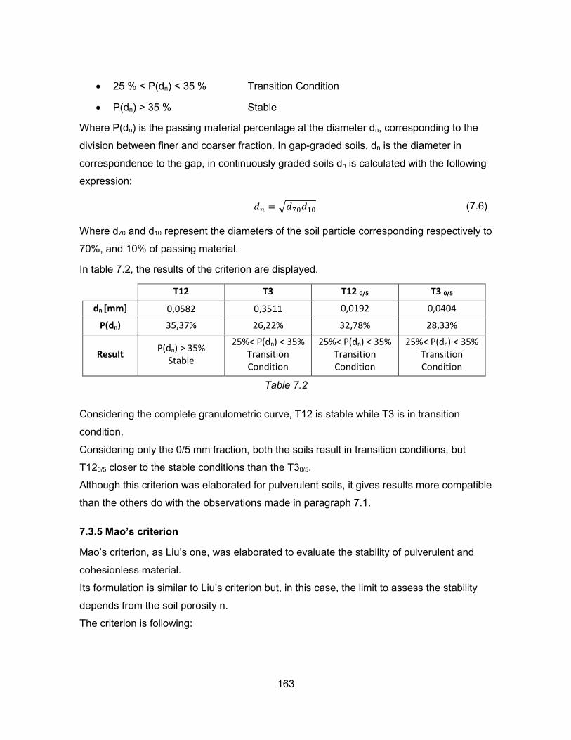
163
25 % < P(dn) < 35 % Transition Condition
P(dn) > 35 % Stable
Where P(dn) is the passing material percentage at the diameter dn, corresponding to the
division between finer and coarser fraction. In gap-graded soils, dn is the diameter in
correspondence to the gap, in continuously graded soils dn is calculated with the following
expression:
𝑑𝑛 = √𝑑70𝑑10 (7.6)
Where d70 and d10 represent the diameters of the soil particle corresponding respectively to
70%, and 10% of passing material.
In table 7.2, the results of the criterion are displayed.
T12 T3 T12 0/5 T3 0/5
dn [mm] 0,0582 0,3511 0,0192 0,0404
P(dn) 35,37% 26,22% 32,78% 28,33%
Result P(dn) > 35%
Stable
25%< P(dn) < 35% Transition Condition
25%< P(dn) < 35% Transition Condition
25%< P(dn) < 35% Transition Condition
Table 7.2
Considering the complete granulometric curve, T12 is stable while T3 is in transition
condition.
Considering only the 0/5 mm fraction, both the soils result in transition conditions, but
T120/5 closer to the stable conditions than the T30/5.
Although this criterion was elaborated for pulverulent soils, it gives results more compatible
than the others do with the observations made in paragraph 7.1.
7.3.5 Mao’s criterion
Mao’s criterion, as Liu’s one, was elaborated to evaluate the stability of pulverulent and
cohesionless material.
Its formulation is similar to Liu’s criterion but, in this case, the limit to assess the stability
depends from the soil porosity n.
The criterion is following:

164
𝑃(𝑑𝑛) <100
4(1 − 𝑛)% Unstable (7.7)
𝑃(𝑑𝑛) ≥100
4(1 − 𝑛)% Stable (7.8)
Where n is the porosity of the soil and P(dn) is the passing material percentage at the
diameter dn, corresponding to the division between finer and coarser fraction. In gap-
graded soils, dn is the diameter in correspondence to the gap, in continuously graded soils
dn is calculated with the following expression:
𝑑𝑛 = 1,3√𝑑85𝑑15 (7.9)
Where d85 and d15 represent the diameters of the soil particle corresponding respectively to
85%, and 15% of passing material.
In order to apply Mao’s criterion, the porosity was calculated as following:
𝑛 = 1 −𝛾𝑑 𝑂𝑃𝑇+2%
𝛾𝑠 (7.10)
Where γd OPT+2% is the dry unit weight (kN/m3) referred to the Proctor test performed with a
content equal to the optimum +2% (chapter 6 paragraph 6.2.1)
γs is the solid unit weight (kN/m3) already calculated in chapter 4 paragraph 4.4.
In table 7.3, the values of γd OPT+2%, γs and n are displayed.
T12 T3 T12 0/5 T3 0/5
γd OPT+2% [kN/m3] 18,77 19,46 18,77 19,46
γs [kN/m3] 26,79 27,36 26,79 27,36
n 0,2995 0,2888 0,2995 0,2888
Table 7.3
In table 7.4, the results of the criterion are presented.

165
T12 T3 T12 0/5 T3 0/5
dn [mm] 0,3251 1,3866 0,0599 0,1387
P(dn) 50,51% 37,11% 47,25% 38,00%
Limit 35,69% 35,15% 35,69% 35,15%
Result Stable Stable Stable Stable
Table 7.4
All the analysed soils are stable according to this criterion and in particular, T12 and T120/5
result more stable than T3 and T30/5.
The results are similar to Liu’s criterion ones. Therefore, in this case too, even if the
criterion was elaborated for pulverulent soils, the results are more compatible with the
observations made in paragraph 7.1. Moreover, this criterion presents the advantage of
taking into account the compaction of the soil through the porosity parameter used in the
limit calculation.
7.3.6 Conclusions on the internal stability criteria
The results obtained from the internal stability criteria are summarised in table 7.5.
T12 T3 T120/5 T30/5
Kezdi (1969)
Unstable Stable
for d>2,5mm Stable
for d>0,025 mm Stable
for d>0,13 mm
Kenney and Lau (1986)
Unstable Unstable Unstable Unstable
Burenkova (1993)
Unstable Stable Unstable Stable
Liu (2005)
Stable Transition condition
Transition condition
Transition condition
Mao (2005)
Stable Stable Stable Stable
Table 7.5
The results depend heavily from the criterion used to verify the internal stability. Therefore,
it is important to choose the right criterion in function of the soil under analysis.
Therefore, the results could not be very affording since the internal stability criteria have

166
been created to study the behaviour of cohesionless soils in view of designing filters, while
T12 and T3 have a high content of fine material.
Kezdi’s criterion (1969) is verified only for the finer fractions but, as stated by Chapuis
(1992) and Wan and Fell (2004), is quite conservative.
The same statement is valid for the Kenney and Lau’s criterion (1986).
Burenkova’s criterion (1993), on the contrary, can classify as stable materials that in reality
are unstable (Wan and Fell, 2004). Moreover, all the results of this analysis are outside the
field studied by the author (figure 7.7).
Liu’s criterion (2005) and Mao’s criterion (2005) have the advantage to consider the nature
of soil. In particular, Mao’s criterion considers the porosity of the soil to calculate the limit
of the criterion. The results of these criteria fit better to the experimental evidence that the
T3 is less stable than T12.
As already mentioned in the chapter introduction, it could be possible that the samples in
the oedo-permeameter and in the hanging column test were subjected to superficial
erosion and not to internal erosion.
In the following paragraphs, external erosion criteria will be applied in order to verify if the
results are more compatible with the experimental observations than the results of the
internal stability criteria.
7.4 EXTERNAL EROSION CRITERIA
Different experiments were carried out to find a relationship between surface erosion and
soil properties. In general, these methods provide an equation to calculate the critical
shear stress, which represents the sensitivity of the soil to erosion. Therefore, when a flux
of water exercises a shear stress higher than the soil characteristic critical value, the soil is
subjected to erosion (Pham, 2008).
In the following paragraphs, some empirical relationships will be applied to study the
susceptibility of T120/5 and T30/5 to external erosion and to analyse the effect of the
bentonite treatments on this matter. For the analysis, only the 0/5 mm fraction
granulometric curve was considered since the tests (Atterberg’s limits, oedo-permeameter
test, hanging column test) were performed on this fraction.
It is necessary to clarify that these relationships are still under study and do not give

167
always results in agree with the real conditions in situ. Hence, in this case too, it is
important to know the limits of these relationships to analyse critically the results.
7.4.1 Analysis of the untreated materials
Shields (1936) was one of the firsts to propose an empirical relationship to determine the
critical shear stress 𝜏𝑐 in function of a diameter of reference. The relationship is the
following:
𝜏𝑐 = 𝑑50 (7.11)
Where 𝜏𝑐 is the critical shear stress (Pa) and d50 is the diameter of the sieve through which
the 50% of grains pass (mm).
Shields’ theory was developed studying uniform, non-cohesive particles for which the
entrainment is due only to gravity, Archimedes’ force and drag forces. Even if for finer and
cohesive particles electromagnetic and electrostatic forces should be considered too,
Shields’ theory was extended to include finer materials (Clark and Wynn, 2006).
Smerdon and Beasley (1961) proposed the following equations:
𝜏𝑐 = 3,54 ∙ 10−28,1∙𝑑50 (7.12)
𝜏𝑐 = 0,493 ∙ 100,0182∙𝐶𝐹 (7.13)
𝜏𝑐 = 0,16 ∙ 𝑃𝐼0,84 (7.14)
Where 𝜏𝑐 is expressed in Pa, d50 is expressed in m, CF is the clay fraction (percentage of
passing material at a reference diameter of 2 µm) and PI is the plastic index of the
material.
Smerdon and Beasley obtained these equations conducting a flume study on eleven
cohesive Missouri soils. The samples were not compacted but only levelled and subjected
to increasing flow rates. The critical shear stress was defined as the shear stress
corresponding to bed failure (Clark and Wynn, 2006).
Julian and Torres (2006) developed the following formula, which takes into account the silt
fraction SC that is the percentage corresponding to the passing material at 0,063 mm:
𝜏𝑐 = 0,1 + 0,1779 ∙ 𝑆𝐶 + 0,0028 ∙ 𝑆𝐶2 − 2,34 ∙ 10−5∙𝑆𝐶3 (7.15)
Where 𝜏𝑐 is expressed in Pa and SC is expressed in percentage.

168
In table 7.6, the obtained results are displayed.
τc [Pa]
T120/5 T30/5
Shields Equation 7.11
0,08 0,34
Smerdon Beasley Equation 7.12
3,52 3,46
Smerdon Beasley Equation 7.13
0,97 0,81
Smerdon Beasley Equation 7.14
1,05 1,08
Julian Torres Equation 7.15
15,03 8,51
Table 7.6
Equation 7.11 (Shields, 1936) gives very low τc values because the extension of the theory
to fine-grained soils is not based on laboratory observations. The method leads to an
underestimation of the critical shear stress and, hence, it is not affordable for fine-grained
soils (Clark and Wynn, 2006).
Since equation 7.12, equation 7.13 and equation 7.14 (Smerdon and Beasley, 1961) were
developed from laboratory tests on cohesive soils, they are more suitable to be used in
this analysis.
According to equation 7.12 and equation 7.13, T120/5 results slightly more resistant to
erosion than T30/5 since it is characterised by a smaller d50 and a higher clay fraction (T120/5
d50=0,08mm and CF=16,21% ; T30/5 d50=0,34mm and CF=11,72%).
Equation 7.14 gives almost equal results for T120/5 and T30/5 since they are characterised
by almost the same plastic index.
Equation 7.15 (Julian and Torres, 2006) gives the higher critical shear stress values. It is
evident that considering the silt fraction SC instead of only the clay fraction CF, the critical
shear stress increases significantly. T120/5 results more resistant than T30/5 since it is
characterised by a higher silt fraction (T120/5 SC=47,87% ; T30/5 SC=31,57%).
Comparing the results of external erosion criteria (table 7.6) with the results of internal
stability criteria (table 7.5), it is possible to notice that the first ones are more in

169
accordance with the experimental observation that T30/5 is more exposed to erosion than
T120/5.
7.4.2 Effect of bentonite treatments
The effect of bentonite treatment will be analysed referring to two methods which refers to
Atterbeg’s limits: Gibbs’ method (1962) and Smerdon and Beasley’s equation 7.14 (1961).
Gibbs (1962) performed laboratory erosion experiments on 45 undisturbed samples
collected from different riverbanks. The results of the experiments brought to the definition
of areas corresponding to different erosion rate in the Casagrande’s chart (figure 7.8).
Figure 7.8
In figure 7.8, the points correspond to the analysed soils. The points corresponding to the
average of T1+T2 0% and of T3 0% are represented too.
T120/5 0% and T30/5 0% are located in the boundary zone between the highest resistance

170
zone and the slight erosion zone.
T120/5 5% and T30/5 5% are located in the slight erosion zone.
T120/5 7% and T30/5 7% are already outside the plastic index range studied by Gibbs. For
this reason, the points corresponding to 12% treatments were not represented.
Smerdon and Beasley’s equation 7.14 (1961) gave the results displayed in figure 7.9 and
table 7.7. In table 7.7 the PI values are displayed too.
Figure 7.9

171
T120-5 T30-5
0% 5% 7% 12% 0% 5% 7% 12%
τc [Pa] 1,049 2,897 4,199 6,031 1,078 2,729 3,212 6,074
PI 9,38% 31,44% 48,87% 75,25% 9,69% 29,27% 35,54% 75,90%
Table 7.7
Increasing the bentonite content, the critical shear stress value τc increases. In fact,
according to equation 7.14, the higher the plasticity index, the higher the resistance to
erosion. For this reason, τc increase has the same trend of the plastic index increase in
function of the bentonite content shown in chapter 4 figure 4.13.
Equation 7.14 explains well the increase of resistance to erosion of T12 and T3 with the
increase of bentonite content but it does not show significant differences between T12 0%
and T3 0%.
7.4.3 Conclusions on the external erosion criteria
No applied method in paragraph 7.4.1 and paragraph 7.4.2 is consolidated.
Regarding equation 7.11 (Shields,1936) and equation 7.12 (Smerdon and Beasley, 1961),
the use of particle reference diameters is not considered suitable for materials containing
high percentage of fine since the contribute of electromagnetic and electrostatic forces
between fine particles are not considered (Briaud et al., 2001).
Regarding Gibbs’ method (1962) and Smerdon and Beasley’s equation 7.14 (1961),
studies by Arulanandam and Perry (1983), Briaud et al. (2001), Wan and Fell (2002) have
shown that there is not a direct correlation between the critical shear stress and the
Atterberg’s limits.
Regarding the relationship between the critical shear stress and the fine percentage
(Smerdon and Beasley’s equation 7.13 and Jules and Torres’ equation 7.15), different
authors have studied this topic but they are not always compatible with the kind of
relationship between the two parameters (Pham, 2008).
Moreover, it must be underlined that the calculation of the critical shear stress of the soil
has been done only in order to have an idea of the soils sensitivity to erosion. In fact, the
shear stress occurring in the oedo-permeameter test and the hanging column test is not
known.
However, even if the applied methods could not be affordable and the results obtained

172
with the different approaches are not always concordant, it is possible to draw two
important qualitative conclusions:
The critical shear stress of T12 is generally higher than the one of T3;
The higher the bentonite rate, the higher the critical shear resistance;
These two conclusions explain the phenomenon observed in the sandbox of the hanging
column test (paragraph 7.1).
7.5 CONCLUSIONS ON SOILS SENSITIVITY TO EROSION
In this chapter, the sensitivity to erosion of two different soils, T12 and T3, was studied
focusing also on the effect of bentonite treatments on this matter.
At first the internal erosion criteria were applied to the samples which appeared more
susceptible to erosion, T12 0% and T3 0%, (paragraph 7.3).
Both the complete granulometric curve and the 0/5 mm fraction curve were used.
Since the internal erosion criteria are generally thought for cohesionless soils the obtained
results are not always in agreement with the expectation. Only Liu’s criterion and Mao’s
criterion (2008) show that the T3 0% is more internally unstable than the T12.
The differences between the results referred to the complete granulometric curve and the
ones referred to the 0/5 mm fraction curve are not significant.
For further analysis, some external erosion criteria were applied to T12 0% and T3 0%,
considering only the 0/5 mm granulometric fraction (paragraph 7.4).
The results are in general more in accordance with the expectations since they show that
T3 0% is more susceptible to erosion than T12 0%.
In paragraph 7.4.3, the effect of bentonite treatment was analysed and it was found that
increasing the bentonite content of the material, the soil resistance to erosion increases.
Finally, it is possible to draw these conclusions:
The problem of fine loss encountered during the hanging column test is due to
superficial erosion more than internal erosion;
The T3 is more subjected to erosion than the T12;
The bentonite treatments increase the resistance of the material.

173
CONCLUSIONS
In this work the effect of bentonite treatments on the hydraulic behaviour of two soils from
a French disposal for low-radioactivity waste (Centre de Stockage de la Manche, CSM)
was analysed.
The two untreated soils (called T12 and T3) are classified respectively as a low plasticity
silt and a sand with high silt content.
T12 and T3 form the clay layer of the CSM cap cover system. In order to guarantee an
impervious long-term cover system, bentonite treatments were proposed.
The influence of the treatment was analysed considering three different percentages
calculated on dry mass: 5%, 7% and 12%.
The bentonite used for the treatment is a calcium activated activated bentonite.
All the analysis were based on the 0/5mm fraction of the untreated and treated soils.
First, the Atteberg limits and the VB value of T12, T3 and their treatments were obtained.
Increasing the bentonite content, the liquid limit, the plastic limit and the plasticity index
increase. The methylene blue adsorption value (VB) increase linearly with the bentonite
content.
The compaction curves of T12, T3 and their treatments were obtained with the standard
Proctor procedure. It was possible to find out that the maximum dry unit weight of the soils
gets lower as the bentonite percentage of the treatment increases.
The hydraulic conductivity of T12, T3 and their treatments in saturated conditions were
obtained with the oedo-permeameter test and empirical relationships.
Increasing the bentonite content, the hydraulic conductivity decreases but there is not a
linear correlation between the two parameters. In particular, the 7% treatment results the
most efficient, since the 12% treatment determines a small additional decrease of
hydraulic conductivity.
The hydraulic conductivity of T12, T3 and their treatments in unsaturated conditions were
studied applying the Van Genuchten model on the experimental results of the hanging
column test.
Increasing suction, the hydraulic conductivity of all the samples decreases but this effect is
less evident for the treated samples.
The samples containing bentonite exhibited swelling and shrinkage during the test and, as

174
a consequence, variation of the dry unit weight. In particular, it was observed that in the
suction interval pF=[1 – 2], the dry unit weight can change even if the volumetric water
content remains constant.
Since during the hanging column test the untreated soil samples, in particular T3, were
subjected to fine particles loss, the effect of bentonite on soil sensitivity to erosion was
analysed referring to internal and external erosion criteria.
The results of the internal erosion criteria were not in accordance with the experimental
results while the external erosion criteria described better the observations made during
the hanging column test.
Hence, it was possible to verify that T3 is more sensitive to erosion than T12 and that
increasing the bentonite content of the material, the soil resistance to erosion increases.
For further analysis, the study of the influence of the soil coarser fraction on the bentonite
treatments is proposed. Moreover, since the unsaturated conditions were studied only with
the hanging column test, it is proposed to analyse more in depth the bentonite treatment
effects on unsaturated hydraulic conductivity, performing tests through which it is possible
to reach higher suction levels.

175
ATTACHMENT
In this section, the data from the hanging column test and the Scilab program used to find
the parameters of Van Genuchten model are reported.

176
HANGING COLUMN TEST – T12 SAMPLES
T12 0% T12 0% T12 5% T12 5% T12 7% T12 7% T12 12% T12 12%
E1 E2 E1 E2 E1 E2 E1 E2
h [cm] 2,97 2,97 3,00 3,03 2,98 3,00 3,02 3,00
d [cm] 5,00 5,00 5,00 5,00 5,00 5,00 5,00 5,00
V [cm3] 58,32 58,32 58,90 59,49 58,51 58,90 59,30 58,90
mring [g] 41,03 41,40 43,26 42,82 55,41 42,80 43,24 43,03
m (string) [g] 1,55 1,56 1,54 1,54 1,52 1,52 1,57 1,54
m (tare) [g] 6,27 6,26 6,44 6,16 5,99 6,29 6,50 3,12
msat (filter) [g] 0,99 0,65 0,92 0,76 1,04 1,14 0,80 0,99
md (filter) [g] 0,46 0,35 0,43 0,37 0,44 0,46 0,42 0,48
mh (soil+ring+filter+tare) [g] 171,50 169,93 164,53 166,84 172,08 163,70 169,46 164,94
md (soil+ring+filter+tare) [g] 155,08 154,11 145,12 147,22 151,56 142,88 141,19 137,96
md (soil) [g] 105,77 104,54 93,45 96,33 88,20 91,81 89,46 89,79
γd [kN/m3] 18,77 18,77 17,51 17,51 16,92 16,92 16,47 16,47
w 14,29% 14,29% 17,91% 17,91% 19,73% 19,73% 21,36% 21,36%
msoil+ring [g] 162,95 162,80 155,46 157,35 163,07 154,12 153,74 153,79
msoil+ring+filter+string [g] 164,78 163,95 157,30 159,09 164,90 155,99 155,55 155,66
mfilter+string [g] 1,83 1,15 1,84 1,74 1,83 1,87 1,81 1,87
γd (soil sample) [kN/m3] 18,14 17,93 15,86 16,19 15,07 15,59 15,09 15,24
Measures made
after the test
Proctor
Values
22/4/14 0:00 minitial [g] 164,78 163,95 157,30 159,09 164,90 155,99 155,55 155,66
mw[g] 16,15 16,86 18,75 18,20 19,46 19,51 21,04 20,97
γd (E) [kN/m3] 18,14 17,93 15,86 16,19 15,07 15,59 15,09 15,24
w 15,27% 16,13% 20,06% 18,89% 22,06% 21,25% 23,52% 23,35%
q 27,69% 28,91% 31,83% 30,59% 33,26% 33,12% 35,48% 35,60%
S 74,80% 81,33% 75,73% 73,03% 74,85% 76,81% 68,48% 72,57%
23/4/14 11:30 msaturation beginning [g] 162,42 161,88 155,65 157,21 163,19 154,36 154,33 154,45
mw[g] 13,08 13,73 16,48 15,76 17,02 17,09 19,26 19,10
γd (E) [kN/m3] 18,14 17,93 15,86 16,19 15,07 15,59 15,09 15,24
w 12,37% 13,13% 17,64% 16,36% 19,30% 18,61% 21,53% 21,27%
q 22,43% 23,54% 27,98% 26,49% 29,09% 29,01% 32,48% 32,43%
S 60,58% 66,23% 66,56% 63,24% 65,46% 67,28% 62,69% 66,10%
28/4/14 14:55 m [g] 170,02 168,06 161,92 164,69 169,57 160,29 161,70 161,52
mw[g] 20,68 19,91 22,75 23,24 23,40 23,02 26,63 26,17
γd (E) [kN/m3] 18,14 17,93 15,86 16,19 15,07 15,59 15,09 15,24
w 19,55% 19,05% 24,34% 24,13% 26,53% 25,07% 29,77% 29,15%
q 35,46% 34,14% 38,62% 39,06% 39,99% 39,08% 44,91% 44,43%
S 95,79% 96,04% 91,88% 93,26% 90,00% 90,63% 86,68% 90,56%
29/4/14 11:25 m [g] 169,95 168,25 161,89 164,44 169,72 160,81 162,09 161,90
mw[g] 20,61 20,10 22,72 22,99 23,55 23,54 27,02 26,55
γd (E) [kN/m3] 18,14 17,93 15,86 16,19 15,07 15,59 15,09 15,24
w 19,49% 19,23% 24,31% 23,87% 26,70% 25,64% 30,20% 29,57%
q 35,34% 34,47% 38,57% 38,64% 40,25% 39,96% 45,57% 45,07%
S 95,46% 96,96% 91,76% 92,26% 90,58% 92,68% 87,95% 91,88%

177
5/5/14 10:54 m [g] 170,29 168,69 162,49 165,74 169,99 161,18 165,15 164,66
mw[g] 20,95 20,54 23,32 24,29 23,82 23,91 30,08 29,31
h [cm] - - - - - - 3,38 3,35
Vswelling [cm3] - - - - - - 66,37 65,78
γd (E) [kN/m3] 18,14 17,93 15,86 16,19 15,07 15,59 13,48 13,65
w 19,81% 19,65% 24,95% 25,22% 27,01% 26,04% 33,62% 32,64%
q 35,93% 35,22% 39,59% 40,83% 40,71% 40,59% 45,32% 44,56%
S 97,04% 99,08% 94,18% 97,47% 91,62% 94,13% 87,48% 90,83%
6/5/14 10:51 m [g] 170,28 168,50 162,83 164,97 169,95 161,59 165,50 164,74
mw[g] 20,94 20,35 23,66 23,52 23,78 24,32 30,43 29,39
h [cm] - - - - - - 3,38 3,35
Vswelling [cm3] - - - - - - 66,37 65,78
γd (E) [kN/m3] 18,14 17,93 15,86 16,19 15,07 15,59 13,48 13,65
w 19,80% 19,47% 25,32% 24,42% 26,96% 26,49% 34,02% 32,73%
q 35,91% 34,90% 40,17% 39,53% 40,64% 41,29% 45,85% 44,68%
S 96,99% 98,17% 95,56% 94,38% 91,46% 95,75% 88,50% 91,08%
12/5/14 10:46 m [g] 170,93 168,78 163,06 165,62 170,60 161,51 167,92 166,51
mw[g] 21,59 20,63 23,89 24,17 24,43 24,24 32,85 31,16
h [cm] - - - - - - 3,44 3,42
Vswelling [cm3] - - - - - - 67,61 67,09
γd (E) [kN/m3] 18,14 17,93 15,86 16,19 15,07 15,59 13,23 13,38
w 20,41% 19,73% 25,56% 25,09% 27,70% 26,40% 36,72% 34,70%
q 37,02% 35,38% 40,56% 40,63% 41,75% 41,15% 48,59% 46,45%
S 100,00% 99,52% 96,49% 96,99% 93,96% 95,43% 93,78% 94,68%
13/5/14 11:20 m [g] 170,77 168,88 163,13 165,60 170,92 161,50 167,70 167,01
mw[g] 21,43 20,73 23,96 24,15 24,75 24,23 32,63 31,66
h [cm] - - - - - - 3,44 3,42
Vswelling [cm3] - - - - - - 67,61 67,09
γd (E) [kN/m3] 18,14 17,93 15,86 16,19 15,07 15,59 13,23 13,38
Beginning of suction w 20,26% 19,83% 25,64% 25,07% 28,06% 26,39% 36,47% 35,26%
PF=0 (-0,001 cm) q 36,75% 35,55% 40,68% 40,59% 42,30% 41,13% 48,26% 47,19%
13/5/14 15:40 S 99,26% 100,00% 96,77% 96,91% 95,19% 95,39% 93,15% 96,20%
19/5/14 11:00 m [g] 170,84 168,70 163,71 166,22 172,07 162,59 169,57 167,51
PF=0 (-0,001 cm) mw[g] 21,50 20,55 24,54 24,77 25,90 25,32 34,50 32,16
h [cm] - - - - - - 3,44 3,42
Vswelling [cm3] - - - - - - 67,61 67,09
γd (E) [kN/m3] 18,14 17,93 15,86 16,19 15,07 15,59 13,23 13,38
Increase of suction w 20,33% 19,66% 26,26% 25,71% 29,37% 27,58% 38,56% 35,82%
PF=0,4 (-2,5 cm) q 36,87% 35,24% 41,66% 41,63% 44,26% 42,98% 51,03% 47,94%
19/5/14 15:30 S 99,58% 99,13% 99,11% 99,40% 99,62% 99,69% 98,49% 97,72%
27/5/14 11:00 m [g] 170,67 168,63 163,93 166,37 172,17 162,67 170,10 168,26
PF=0,4 (-2,5 cm) mw[g] 21,33 20,48 24,76 24,92 26,00 25,40 35,03 32,91
h [cm] - - - - - - 3,44 3,42
Vswelling [cm3] - - - - - - 67,61 67,09
γd (E) [kN/m3] 18,14 17,93 15,86 16,19 15,07 15,59 13,23 13,38
Increase of suction w 20,17% 19,59% 26,50% 25,87% 29,48% 27,67% 39,16% 36,65%
PF=1 (-10 cm) q 36,58% 35,12% 42,03% 41,89% 44,44% 43,12% 51,81% 49,06%
27/5/14 11:30 S 98,80% 98,79% 100,00% 100,00% 100,00% 100,00% 100,00% 100,00%

178
2/6/14 11:00 m [g] 168,88 167,17 161,64 164,45 169,39 160,70 168,03 166,04
PF=1 (-10 cm) mw[g] 19,54 19,02 22,47 23,00 23,22 23,43 32,96 30,69
1°measure h [cm] - - 3,033 3,103 3,083 3,117 3,50 3,42
Vswelling [cm3] - - 59,559 60,934 60,541 61,196 68,79 67,22
γd (E) [kN/m3] 18,14 17,93 15,69 15,81 14,57 15,00 13,01 13,36
w 18,47% 18,19% 24,04% 23,88% 26,33% 25,52% 36,84% 34,18%
q 33,51% 32,62% 37,73% 37,75% 38,35% 38,29% 47,92% 45,66%
S 90,50% 91,75% 89,75% 90,11% 86,31% 88,79% 92,48% 93,07%
3/6/14 11:46 m [g] 168,79 167,03 161,52 164,37 169,29 160,59 167,91 165,92
PF=1 (-10 cm) mw[g] 19,45 18,88 22,35 22,92 23,12 23,32 32,84 30,57
2°measure h [cm] - - 3,033 3,103 3,083 3,117 3,50 3,42
Vswelling [cm3] - - 59,559 60,934 60,541 61,196 68,79 67,22
γd (E) [kN/m3] 18,14 17,93 15,69 15,81 14,57 15,00 13,01 13,36
w 18,39% 18,06% 23,92% 23,79% 26,21% 25,40% 36,71% 34,05%
q 33,35% 32,38% 37,53% 37,61% 38,19% 38,11% 47,74% 45,48%
S 90,09% 91,08% 89,27% 89,80% 85,94% 88,37% 92,14% 92,71%
q1-q2 0,15% 0,24% 0,20% 0,13% 0,17% 0,18% 0,17% 0,18%
Ok No! No! Ok Ok Ok Ok Ok
4/6/14 11:30 m [g] 168,64 166,90 161,42 164,27 169,15 160,50 167,79 165,81
PF=1 (-10 cm) mw[g] 19,30 18,75 22,25 22,82 22,98 23,23 32,72 30,46
3°measure h [cm] - - 3,033 3,103 3,083 3,117 3,50 3,42
Vswelling [cm3] - - 59,559 60,934 60,541 61,196 68,79 67,22
γd (E) [kN/m3] 18,14 17,93 15,69 15,81 14,57 15,00 13,01 13,36
Increase of suction w 18,25% 17,94% 23,81% 23,69% 26,05% 25,30% 36,58% 33,92%
PF=1,5 (-31,6 cm) q 33,10% 32,15% 37,36% 37,45% 37,96% 37,96% 47,57% 45,32%
4/6/14 14:30 S 89,39% 90,45% 88,88% 89,41% 85,42% 88,03% 91,81% 92,38%
q2-q3 0,26% 0,22% 0,17% 0,16% 0,23% 0,15% 0,17% 0,16%
No! No! Ok Ok No! Ok Ok Ok
11/6/14 11:50 m [g] 168,20 166,62 161,06 163,87 168,97 160,27 167,30 165,43
PF=1,5 (-31,6 cm) mw[g] 18,86 18,47 21,89 22,42 22,80 23,00 32,23 30,08
1°measure h [cm] - - 3,033 3,103 3,083 3,117 3,51 3,44
Vswelling [cm3] - - 59,559 60,934 60,541 61,196 68,85 67,48
γd (E) [kN/m3] 18,14 17,93 15,69 15,81 14,57 15,00 12,99 13,31
w 17,83% 17,67% 23,42% 23,27% 25,85% 25,05% 36,03% 33,50%
q 32,34% 31,67% 36,75% 36,79% 37,66% 37,58% 46,81% 44,58%
S 87,36% 89,10% 87,44% 87,84% 84,75% 87,16% 90,35% 90,87%
12/6/14 11:05 m [g] 168,10 166,52 160,93 163,75 168,87 160,14 167,04 165,21
PF=1,5 (-31,6 cm) mw[g] 18,76 18,37 21,76 22,30 22,70 22,87 31,97 29,86
2°measure h [cm] - - 3,033 3,103 3,083 3,117 3,51 3,44
Vswelling [cm3] - - 59,559 60,934 60,541 61,196 68,85 67,48
γd (E) [kN/m3] 18,14 17,93 15,69 15,81 14,57 15,00 12,99 13,31
w 17,74% 17,57% 23,29% 23,15% 25,74% 24,91% 35,74% 33,26%
q 32,17% 31,50% 36,53% 36,60% 37,50% 37,37% 46,43% 44,25%
S 86,89% 88,62% 86,92% 87,37% 84,38% 86,67% 89,62% 90,20%
q1-q2 0,17% 0,17% 0,22% 0,20% 0,17% 0,21% 0,38% 0,33%
Ok Ok No! Ok Ok No! No! No!
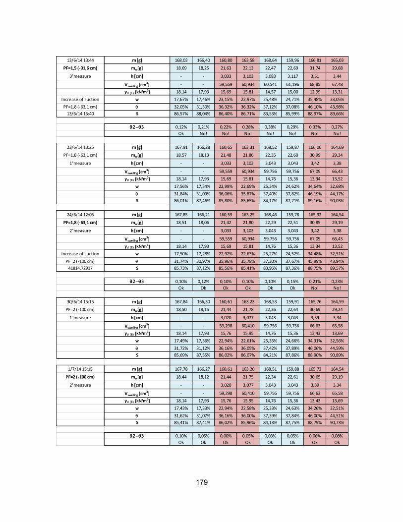
179
13/6/14 13:44 m [g] 168,03 166,40 160,80 163,58 168,64 159,96 166,81 165,03
PF=1,5 (-31,6 cm) mw[g] 18,69 18,25 21,63 22,13 22,47 22,69 31,74 29,68
3°measure h [cm] - - 3,033 3,103 3,083 3,117 3,51 3,44
Vswelling [cm3] - - 59,559 60,934 60,541 61,196 68,85 67,48
γd (E) [kN/m3] 18,14 17,93 15,69 15,81 14,57 15,00 12,99 13,31
Increase of suction w 17,67% 17,46% 23,15% 22,97% 25,48% 24,71% 35,48% 33,05%
PF=1,8 (-63,1 cm) q 32,05% 31,30% 36,32% 36,32% 37,12% 37,08% 46,10% 43,98%
13/6/14 15:40 S 86,57% 88,04% 86,40% 86,71% 83,53% 85,99% 88,97% 89,66%
q2-q3 0,12% 0,21% 0,22% 0,28% 0,38% 0,29% 0,33% 0,27%
Ok No! No! No! No! No! No! No!
23/6/14 13:25 m [g] 167,91 166,28 160,65 163,31 168,52 159,87 166,06 164,69
PF=1,8 (-63,1 cm) mw[g] 18,57 18,13 21,48 21,86 22,35 22,60 30,99 29,34
1°measure h [cm] - - 3,033 3,103 3,043 3,043 3,42 3,38
Vswelling [cm3] - - 59,559 60,934 59,756 59,756 67,09 66,43
γd (E) [kN/m3] 18,14 17,93 15,69 15,81 14,76 15,36 13,34 13,52
w 17,56% 17,34% 22,99% 22,69% 25,34% 24,62% 34,64% 32,68%
q 31,84% 31,09% 36,06% 35,87% 37,40% 37,82% 46,19% 44,17%
S 86,01% 87,46% 85,80% 85,65% 84,17% 87,71% 89,16% 90,03%
24/6/14 12:05 m [g] 167,85 166,21 160,59 163,25 168,46 159,78 165,92 164,54
PF=1,8 (-63,1 cm) mw[g] 18,51 18,06 21,42 21,80 22,29 22,51 30,85 29,19
2°measure h [cm] - - 3,033 3,103 3,043 3,043 3,42 3,38
Vswelling [cm3] - - 59,559 60,934 59,756 59,756 67,09 66,43
γd (E) [kN/m3] 18,14 17,93 15,69 15,81 14,76 15,36 13,34 13,52
Increase of suction w 17,50% 17,28% 22,92% 22,63% 25,27% 24,52% 34,48% 32,51%
PF=2 (-100 cm) q 31,74% 30,97% 35,96% 35,78% 37,30% 37,67% 45,99% 43,94%
41814,72917 S 85,73% 87,12% 85,56% 85,41% 83,95% 87,36% 88,75% 89,57%
q2-q3 0,10% 0,12% 0,10% 0,10% 0,10% 0,15% 0,21% 0,23%
Ok Ok Ok Ok Ok Ok No! No!
30/6/14 15:15 m [g] 167,84 166,30 160,61 163,23 168,53 159,91 165,76 164,59
PF=2 (-100 cm) mw[g] 18,50 18,15 21,44 21,78 22,36 22,64 30,69 29,24
1°measure h [cm] - - 3,020 3,077 3,043 3,043 3,39 3,34
Vswelling [cm3] - - 59,298 60,410 59,756 59,756 66,63 65,58
γd (E) [kN/m3] 18,14 17,93 15,76 15,95 14,76 15,36 13,43 13,69
w 17,49% 17,36% 22,94% 22,61% 25,35% 24,66% 34,31% 32,56%
q 31,72% 31,12% 36,16% 36,05% 37,42% 37,89% 46,06% 44,59%
S 85,69% 87,55% 86,02% 86,07% 84,21% 87,86% 88,90% 90,89%
1/7/14 15:15 m [g] 167,78 166,27 160,61 163,20 168,51 159,88 165,72 164,54
PF=2 (-100 cm) mw[g] 18,44 18,12 21,44 21,75 22,34 22,61 30,65 29,19
2°measure h [cm] - - 3,020 3,077 3,043 3,043 3,39 3,34
Vswelling [cm3] - - 59,298 60,410 59,756 59,756 66,63 65,58
γd (E) [kN/m3] 18,14 17,93 15,76 15,95 14,76 15,36 13,43 13,69
w 17,43% 17,33% 22,94% 22,58% 25,33% 24,63% 34,26% 32,51%
q 31,62% 31,07% 36,16% 36,00% 37,39% 37,84% 46,00% 44,51%
S 85,41% 87,41% 86,02% 85,96% 84,13% 87,75% 88,79% 90,73%
q2-q3 0,10% 0,05% 0,00% 0,05% 0,03% 0,05% 0,06% 0,08%
Ok Ok Ok Ok Ok Ok Ok Ok

180
HANGING COLUMN TEST – T3 SAMPLES
T3 0% T3 0% T3 5% T3 7% T3 7% T3 12% T3 12%
E1 E2 E1 E1 E2 E1 E2
h [cm] 2,96 3,01 3,03 2,99 2,98 3,00 3,03
d [cm] 5,00 5,00 5,00 5,00 5,00 5,00 5,00
V [cm3] 58,12 59,10 59,49 58,71 58,51 58,90 59,49
mring [g] 42,39 41,92 43,55 41,35 42,77 43,25 41,80
m (string) [g] 1,57 1,58 1,55 1,54 1,55 1,56 1,54
m (tare) [g] 3,17 3,32 6,55 6,42 6,46 6,38 6,50
msat (filter) [g] 0,93 1,04 1,12 1,07 1,10 0,68 0,79
md (filter) [g] 0,48 0,54 0,53 0,52 0,49 0,37 0,36
mh (soil+ring+filter+tare) [g] 167,14 172,05 168,98 168,00 167,06 175,42 175,65
md (soil+ring+filter+tare) [g] 152,31 156,54 150,25 147,48 146,83 146,41 147,19
md (soil) [g] 104,70 109,18 98,07 97,65 95,56 94,85 96,99
γd [kN/m3] 19,46 19,46 18,13 17,95 17,95 17,40 17,40
w 12,63% 12,63% 16,77% 17,40% 17,40% 18,38% 18,38%
msoil+ring [g] 162,03 166,84 159,23 158,20 156,57 157,87 158,13
msoil+ring+filter+string [g] 163,89 168,78 161,20 160,09 158,47 159,58 159,79
mfilter+string [g] 1,86 1,94 1,97 1,89 1,90 1,71 1,66
γd (soil sample) [kN/m3] 18,01 18,47 16,48 16,63 16,33 16,10 16,30
Measures made
after the test
Proctor
Values
22/4/14 0:00 minitial [g] 163,89 168,78 161,20 160,09 158,47 159,58 159,79
mw[g] 14,94 15,74 17,61 19,20 18,24 19,77 19,34
γd (E) [kN/m3] 18,01 18,47 16,48 16,63 16,33 16,10 16,30
w 14,27% 14,42% 17,96% 19,66% 19,09% 20,84% 19,94%
q 25,71% 26,63% 29,60% 32,70% 31,17% 33,56% 32,51%
S 67,27% 73,86% 71,91% 71,75% 71,50% 62,31% 62,22%
23/4/14 11:30 msaturation beginning [g] 162,81 167,67 160,06 159,34 157,76 159,07 159,25
mw[g] 13,22 13,95 15,77 17,73 16,78 18,73 18,13
γd (E) [kN/m3] 18,01 18,47 16,48 16,63 16,33 16,10 16,30
w 12,63% 12,78% 16,08% 18,16% 17,56% 19,75% 18,69%
q 22,75% 23,60% 26,51% 30,20% 28,68% 31,80% 30,47%
S 59,52% 65,46% 64,39% 66,26% 65,78% 59,04% 58,33%
28/4/14 14:55 m [g] 170,00 173,88 167,41 166,03 163,87 166,87 166,72
mw[g] 20,41 20,16 23,12 24,42 22,89 26,53 25,60
γd (E) [kN/m3] 18,01 18,47 16,48 16,63 16,33 16,10 16,30
w 19,49% 18,46% 23,57% 25,01% 23,95% 27,97% 26,39%
q 35,12% 34,11% 38,86% 41,60% 39,12% 45,04% 43,03%
S 91,90% 94,60% 94,41% 91,26% 89,73% 83,62% 82,37%

181
29/4/14 11:25 m [g] 170,14 174,14 167,44 166,43 164,20 167,01 167,14
mw[g] 20,55 20,42 23,15 24,82 23,22 26,67 26,02
γd (E) [kN/m3] 18,01 18,47 16,48 16,63 16,33 16,10 16,30
w 19,63% 18,70% 23,61% 25,42% 24,30% 28,12% 26,83%
q 35,36% 34,55% 38,91% 42,28% 39,68% 45,28% 43,74%
S 92,53% 95,82% 94,53% 92,75% 91,02% 84,06% 83,72%
5/5/14 10:54 m [g] 170,64 174,40 166,76 166,17 164,32 170,15 169,83
mw[g] 21,05 20,68 22,47 24,56 23,34 29,81 28,71
h [cm] - - - - - 3,43 3,44
Vswelling [cm3] - - - - - 67,41 67,54
γd (E) [kN/m3] 18,01 18,47 16,48 16,63 16,33 14,07 14,36
w 20,11% 18,94% 22,91% 25,15% 24,42% 31,43% 29,60%
q 36,22% 34,99% 37,77% 41,83% 39,89% 44,22% 42,51%
S 94,78% 97,04% 91,75% 91,78% 91,49% 82,10% 81,36%
6/5/14 10:51 m [g] 171,00 174,56 166,96 166,95 164,23 170,67 170,50
mw[g] 21,41 20,84 22,67 25,34 23,25 30,33 29,38
h [cm] - - - - - 3,43 3,44
Vswelling [cm3] - - - - - 67,41 67,54
γd (E) [kN/m3] 18,01 18,47 16,48 16,63 16,33 14,07 14,36
w 20,45% 19,09% 23,12% 25,95% 24,33% 31,98% 30,29%
q 36,84% 35,26% 38,10% 43,16% 39,74% 44,99% 43,50%
S 96,40% 97,79% 92,57% 94,69% 91,14% 83,53% 83,26%
12/5/14 10:46 m [g] 171,35 174,82 167,33 167,07 164,72 173,03 173,69
mw[g] 21,76 21,10 23,04 25,46 23,74 32,69 32,57
h [cm] - - - - - 3,52 3,57
Vswelling [cm3] - - - - - 69,05 70,10
γd (E) [kN/m3] 18,01 18,47 16,48 16,63 16,33 13,74 13,84
w 20,78% 19,33% 23,49% 26,07% 24,84% 34,46% 33,58%
q 37,44% 35,70% 38,73% 43,37% 40,57% 47,34% 46,46%
S 97,97% 99,01% 94,08% 95,14% 93,06% 87,90% 88,94%
13/5/14 11:20 m [g] 171,56 174,79 168,19 167,17 165,17 173,23 174,36
mw[g] 21,97 21,07 23,90 25,56 24,19 32,89 33,24
h [cm] - - - - - 3,52 3,57
Vswelling [cm3] - - - - - 69,05 70,10
γd (E) [kN/m3] 18,01 18,47 16,48 16,63 16,33 13,74 13,84
Beginning of suction w 20,98% 19,30% 24,37% 26,18% 25,31% 34,68% 34,27%
PF=0 (-0,001 cm) q 37,80% 35,65% 40,17% 43,54% 41,34% 47,63% 47,42%
13/5/14 15:40 S 98,92% 98,87% 97,59% 95,52% 94,83% 88,44% 90,77%
19/5/14 11:00 m [g] 171,80 174,94 167,90 167,76 165,72 175,82 176,31
PF=0 (-0,001 cm) mw[g] 22,21 21,22 23,61 26,15 24,74 35,48 35,19
h [cm] - - - - - 3,52 3,57
Vswelling [cm3] - - - - - 69,05 70,10
γd (E) [kN/m3] 18,01 18,47 16,48 16,63 16,33 13,74 13,84
Increase of suction w 21,21% 19,44% 24,07% 26,78% 25,89% 37,41% 36,28%
PF=0,4 (-2,5 cm) q 38,21% 35,90% 39,68% 44,54% 42,28% 51,38% 50,20%
19/5/14 15:30 S 100,00% 99,58% 96,41% 97,72% 96,98% 95,40% 96,10%

182
27/5/14 11:00 m [g] 171,67 175,03 168,78 168,37 166,49 177,53 177,74
PF=0,4 (-2,5 cm) mw[g] 22,08 21,31 24,49 26,76 25,51 37,19 36,62
h [cm] - - - - - 3,52 3,57
Vswelling [cm3] - - - - - 69,05 70,10
γd (E) [kN/m3] 18,01 18,47 16,48 16,63 16,33 13,74 13,84
Increase of suction w 21,09% 19,52% 24,97% 27,40% 26,70% 39,21% 37,76%
PF=1 (-10 cm) q 37,99% 36,06% 41,16% 45,58% 43,60% 53,86% 52,24%
27/5/14 11:30 S 99,41% 100,00% 100,00% 100,00% 100,00% 100,00% 100,00%
2/6/14 11:00 m [g] 168,07 172,59 166,39 165,83 164,27 175,06 175,52
PF=1 (-10 cm) mw[g] 18,48 18,87 22,10 24,22 23,29 34,72 34,40
1°measure h [cm] - - 3,090 3,123 3,117 3,68 3,71
Vswelling [cm3] - - 60,672 61,327 61,196 72,32 72,91
γd (E) [kN/m3] 18,01 18,47 16,16 15,92 15,62 13,11 13,30
w 17,65% 17,28% 22,53% 24,80% 24,37% 36,61% 35,47%
q 31,80% 31,93% 36,43% 39,49% 38,06% 48,01% 47,18%
S 83,21% 88,55% 88,49% 86,64% 87,29% 89,13% 90,31%
3/6/14 11:46 m [g] 167,70 172,42 166,23 165,40 164,18 174,88 175,24
PF=1 (-10 cm) mw[g] 18,11 18,70 21,94 23,79 23,20 34,54 34,12
2°measure h [cm] - - 3,090 3,123 3,117 3,68 3,71
Vswelling [cm3] - - 60,672 61,327 61,196 72,32 72,91
γd (E) [kN/m3] 18,01 18,47 16,16 15,92 15,62 13,11 13,30
w 17,30% 17,13% 22,37% 24,36% 24,28% 36,42% 35,18%
q 31,16% 31,64% 36,16% 38,79% 37,91% 47,76% 46,80%
S 81,54% 87,75% 87,85% 85,11% 86,96% 88,67% 89,58%
q1-q2 0,64% 0,29% 0,26% 0,70% 0,15% 0,25% 0,38%
No! No! No! No! Ok No! No!
4/6/14 11:30 m [g] 167,44 172,13 166,06 165,30 164,08 174,75 174,96
PF=1 (-10 cm) mw[g] 17,85 18,41 21,77 23,69 23,10 34,41 33,84
3°measure h [cm] - - 3,090 3,123 3,117 3,68 3,71
Vswelling [cm3] - - 60,672 61,327 61,196 72,32 72,91
γd (E) [kN/m3] 18,01 18,47 16,16 15,92 15,62 13,11 13,30
Increase of suction w 17,05% 16,86% 22,20% 24,26% 24,17% 36,28% 34,89%
PF=1,5 (-31,6 cm) q 30,71% 31,15% 35,88% 38,63% 37,75% 47,58% 46,41%
4/6/14 14:30 S 80,37% 86,39% 87,17% 84,75% 86,58% 88,34% 88,84%
q2-q3 0,45% 0,49% 0,28% 0,16% 0,16% 0,18% 0,38%
No! No! No! Ok Ok Ok No!

183
11/6/14 11:50 m [g] 167,24 171,77 165,62 164,74 163,77 173,86 173,94
PF=1,5 (-31,6 cm) mw[g] 17,65 18,05 21,33 23,13 22,79 33,52 32,82
1°measure h [cm] - - 3,090 3,123 3,117 3,67 3,69
Vswelling [cm3] - - 60,672 61,327 61,196 72,06 72,45
γd (E) [kN/m3] 18,01 18,47 16,16 15,92 15,62 13,16 13,39
w 16,86% 16,53% 21,75% 23,69% 23,85% 35,34% 33,84%
q 30,37% 30,54% 35,16% 37,72% 37,24% 46,52% 45,30%
S 79,47% 84,70% 85,41% 82,75% 85,42% 86,37% 86,71%
12/6/14 11:05 m [g] 167,05 171,61 165,41 164,48 163,55 173,49 173,52
PF=1,5 (-31,6 cm) mw[g] 17,46 17,89 21,12 22,87 22,57 33,15 32,40
2°measure h [cm] - - 3,090 3,123 3,117 3,67 3,69
Vswelling [cm3] - - 60,672 61,327 61,196 72,06 72,45
γd (E) [kN/m3] 18,01 18,47 16,16 15,92 15,62 13,16 13,39
w 16,68% 16,39% 21,54% 23,42% 23,62% 34,95% 33,41%
q 30,04% 30,27% 34,81% 37,29% 36,88% 46,00% 44,72%
S 78,61% 83,95% 84,56% 81,81% 84,60% 85,41% 85,60%
q1-q2 0,33% 0,27% 0,35% 0,42% 0,36% 0,51% 0,58%
No! No! No! No! No! No! No!
13/6/14 13:44 m [g] 166,99 171,55 165,37 164,32 163,39 173,17 173,30
PF=1,5 (-31,6 cm) mw[g] 17,40 17,83 21,08 22,71 22,41 32,83 32,18
3°measure h [cm] - - 3,090 3,123 3,117 3,67 3,69
Vswelling [cm3] - - 60,672 61,327 61,196 72,06 72,45
γd (E) [kN/m3] 18,01 18,47 16,16 15,92 15,62 13,16 13,39
Increase of suction w 16,62% 16,33% 21,49% 23,26% 23,45% 34,61% 33,18%
PF=1,8 (-63,1 cm) q 29,94% 30,17% 34,74% 37,03% 36,62% 45,56% 44,42%
13/6/14 15:40 S 78,34% 83,67% 84,40% 81,24% 84,00% 84,59% 85,02%
q2-q3 0,10% 0,10% 0,07% 0,26% 0,26% 0,44% 0,30%
Ok Ok Ok No! No! No! No!

184
23/6/14 13:25 m [g] 166,68 171,39 165,07 164,22 163,10 172,03 172,20
PF=1,8 (-63,1 cm) mw[g] 17,09 17,67 20,78 22,61 22,12 31,69 31,08
1°measure h [cm] - - 3,090 3,067 3,083 3,54 3,57
Vswelling [cm3] - - 60,672 60,214 60,541 69,57 70,10
γd (E) [kN/m3] 18,01 18,47 16,16 16,22 15,78 13,63 13,84
w 16,32% 16,18% 21,19% 23,15% 23,15% 33,41% 32,04%
q 29,40% 29,90% 34,25% 37,55% 36,54% 45,55% 44,34%
S 76,95% 82,92% 83,20% 82,38% 83,81% 84,57% 84,87%
24/6/14 12:05 m [g] 166,56 171,29 164,96 164,09 163,01 171,84 172,02
PF=1,8 (-63,1 cm) mw[g] 16,97 17,57 20,67 22,48 22,03 31,50 30,90
2°measure h [cm] - - 3,090 3,067 3,083 3,54 3,57
Vswelling [cm3] - - 60,672 60,214 60,541 69,57 70,10
γd (E) [kN/m3] 18,01 18,47 16,16 16,22 15,78 13,63 13,84
Increase of suction w 16,21% 16,09% 21,08% 23,02% 23,05% 33,21% 31,86%
PF=2 (-100 cm) q 29,20% 29,73% 34,07% 37,33% 36,39% 45,28% 44,08%
41814,72917 S 76,41% 82,45% 82,76% 81,91% 83,46% 84,06% 84,38%
q2-q3 0,21% 0,17% 0,18% 0,22% 0,15% 0,27% 0,26%
No! Ok Ok No! Ok No! No!
30/6/14 15:15 m [g] 166,66 171,36 164,94 164,20 163,15 171,84 171,88
PF=2 (-100 cm) mw[g] 17,07 17,64 20,65 22,59 22,17 31,50 30,76
1°measure h [cm] - - 3,073 3,050 3,043 3,55 3,53
Vswelling [cm3] - - 60,345 59,887 59,756 69,64 69,31
γd (E) [kN/m3] 18,01 18,47 16,25 16,31 15,99 13,62 13,99
w 16,30% 16,16% 21,06% 23,13% 23,20% 33,21% 31,71%
q 29,37% 29,85% 34,22% 37,72% 37,10% 45,23% 44,38%
S 76,86% 82,78% 83,13% 82,76% 85,10% 83,98% 84,95%
1/7/14 15:15 m [g] 166,62 171,33 164,89 164,16 163,12 171,78 171,84
PF=2 (-100 cm) mw[g] 17,03 17,61 20,60 22,55 22,14 31,44 30,72
2°measure h [cm] - - 3,073 3,050 3,043 3,55 3,53
Vswelling [cm3] - - 60,345 59,887 59,756 69,64 69,31
γd (E) [kN/m3] 18,01 18,47 16,25 16,31 15,99 13,62 13,99
w 16,27% 16,13% 21,01% 23,09% 23,17% 33,15% 31,67%
q 29,30% 29,80% 34,14% 37,65% 37,05% 45,15% 44,32%
S 76,68% 82,64% 82,93% 82,61% 84,98% 83,82% 84,84%
q2-q3 0,07% 0,05% 0,08% 0,07% 0,05% 0,09% 0,06%
Ok Ok Ok Ok Ok Ok Ok

185
SWELLING MEASURES – T12
SWELLING MEASURES – T3
θ VARIATION DURING THE HANGING COLUMN TEST – T12
T12 5% T12 5% T12 7% T12 7% T12 12% T12 12%
E1 E2 E1 E2 E1 E2
Initial Value 3,00 3,03 2,98 3,00 3,02 3,00
1st Measure - - - - 3,38 3,35
2nd Measure - - - - 3,44 3,42
3rd Measure - - - - 3,50 3,42
4th Measure - - 3,08 3,12 3,51 3,44
5th Measure 3,03 3,10 3,04 3,04 3,42 3,38
6th Measure 3,02 3,08 3,04 3,04 3,39 3,34
h [mm]
T3 5% T3 7% T3 7% T3 12% T3 12%
E1 E1 E2 E1 E2
Initial Value 3,03 2,99 2,98 3 3,03
1st Measure - - - 3,43 3,44
2nd Measure - - - 3,52 3,57
3rd Measure - - - 3,68 3,71
4th Measure - 3,12 3,12 3,67 3,69
5th Measure 3,09 3,07 3,08 3,54 3,57
6th Measure 3,07 3,05 3,04 3,55 3,53
h [mm]
T12 0% T12 0% T12 5% T12 5% T12 7% T12 7% T12 12% T12 12%
E1 E2 E1 E2 E1 E2 E1 E2
0,01 0,00 37,02% 35,55% 42,03% 41,89% 44,44% 43,12% 51,81% 49,06%
0,03 0,40 36,58% 35,12% 42,03% 41,89% 44,44% 43,12% 51,81% 49,06%
0,10 1,00 33,51% 32,62% 37,73% 37,75% 38,35% 38,29% 47,92% 45,66%
0,32 1,50 33,35% 32,38% 37,53% 37,61% 38,19% 38,11% 47,74% 45,48%
0,63 1,80 33,10% 32,15% 37,36% 37,45% 37,96% 37,96% 47,57% 45,32%
1,00 2,00 32,34% 31,67% 36,75% 36,79% 37,66% 37,58% 46,81% 44,58%
h [m] pf

186
θ VARIATION DURING THE HANGING COLUMN TEST – T3
S VARIATION DURING THE HANGING COLUMN TEST – T12
S VARIATION DURING THE HANGING COLUMN TEST – T3
T3 0% T3 0% T3 5% T3 7% T3 7% T3 12% T3 12%
E1 E2 E1 E1 E2 E1 E2
0,01 0,00 38,21% 36,06% 41,16% 45,58% 43,60% 53,86% 52,24%
0,03 0,40 37,99% 36,06% 41,16% 45,58% 43,60% 53,86% 52,24%
0,10 1,00 31,80% 31,93% 36,43% 39,49% 38,06% 48,01% 47,18%
0,32 1,50 31,16% 31,64% 36,16% 38,79% 37,91% 47,76% 46,80%
0,63 1,80 30,71% 31,15% 35,88% 38,63% 37,75% 47,58% 46,41%
1,00 2,00 30,37% 30,54% 35,16% 37,72% 37,24% 46,52% 45,30%
h [m] pf
T12 0% T12 0% T12 5% T12 5% T12 7% T12 7% T12 12% T12 12%
E1 E2 E1 E2 E1 E2 E1 E2
0,0100 0,00 100,00% 100,00% 100,00% 100,00% 100,00% 100,00% 100,00% 100,00%
0,0251 0,4 98,80% 98,79% 100,00% 100,00% 100,00% 100,00% 100,00% 100,00%
0,1000 1,00 90,50% 91,75% 89,75% 90,11% 86,31% 88,79% 92,48% 93,07%
0,3162 1,50 90,09% 91,08% 89,27% 89,80% 85,94% 88,37% 92,14% 92,71%
0,6310 1,80 89,39% 90,45% 88,88% 89,41% 85,42% 88,03% 91,81% 92,38%
1,0000 2,00 87,36% 89,10% 87,44% 87,84% 84,75% 87,16% 90,35% 90,87%
h [m] pf
T3 0% T3 0% T3 5% T3 7% T3 7% T3 12% T3 12%
E1 E2 E1 E1 E2 E1 E2
0,0100 0,00 100,00% 100,00% 100,00% 100,00% 100,00% 100,00% 100,00%
0,0251 0,4 99,41% 100,00% 100,00% 100,00% 100,00% 100,00% 100,00%
0,1000 1,00 83,21% 88,55% 88,49% 86,64% 87,29% 89,13% 90,31%
0,3162 1,50 81,54% 87,75% 87,85% 85,11% 86,96% 88,67% 89,58%
0,6310 1,80 80,37% 86,39% 87,17% 84,75% 86,58% 88,34% 88,84%
1,0000 2,00 79,47% 84,70% 85,41% 82,75% 85,42% 86,37% 86,71%
h [m] pf

187
PARAMETERS OF VAN GENUCHTEN MODEL – Scilab program
function [ALPHAopt, Mopt, RMSmin, Nopt, entrant]=ParametreVG() stacksize('max') format('v',20) fichier=input("entrer nom du fichier ","string") entrant=read(fichier,-1,2) taille=size(entrant) nbrcombinaison=input("entre le nombre de couple alpha et n à tester = ") nbrpoints=taille(1,1) alphamin=0 alphamax=1 "RESULtab=ones(3,nbrcombinaison)" ALPHAopt=999 Mopt=999 RMSmin=999999 "Z=zeros(1,nbrcombinaison)" "Y=zeros(1,nbrcombinaison)" "X=zeros(1,nbrcombinaison)" modele=ones(nbrpoints,1) for i=1:nbrcombinaison RMS=0 alpha=alphamin+rand()*(alphamax-alphamin) m=rand() for j=1:nbrpoints modele(j,1)=(1+((alpha)*(entrant(j,1)))^(1/(1-m)))^(-m) RMS=RMS+(entrant(j,2)-modele(j,1))^2 end RMS=sqrt(RMS/nbrpoints) "RESULtab(1,i)=RMS" "RESULtab(2,i)=alpha"

188
"RESULtab(3,i)=m" "Z(1,i)=RMS" "Y(1,i)=alpha" "X(1,i)=1/(1-m)" if RMS<RMSmin then RMSmin=RMS ALPHAopt=alpha Mopt=m Nopt=1/(1-m) end end "param3d(X,Y,Z)" endfunction

189
BIBLIOGRAPHY
Aldaeef A.A., Rayhani M.T., 2014, Hydraulic performance of compacted clay liners under
combined temperature and leachate exposures, Department of Civil and Environmental
Engineering, Carleton University, Ottawa, ON, Canada.
ANDRA, 2009, Le Centre de stockage de la Manche: 40 ans d’histoire, www.andra.fr.
ANDRA, 2011, The deep geologichal disposal concept as developed by Andra.
ANDRA, 2012a, National inventory of radioactive Materials and Waste, Synthesis report.
ANDRA, 2012b, Le journal de l’Andra, Edition de la Manche, n°10, page 3.
Arrêté du 30 décembre 2002, Stockage de déchets dangereux.
Barral C., 2008, Etude des transferts d’eau et de gaz dans les geomateriaux argileux
utilises dans les couvertures des installations de stockage de dechets non dangereux,
PhD thesis.
Borrmann F., 2010, Management of very low level radioactive waste in Europe –
application of clearance and the alternatives, IAEA Regional Workshop on the Release of
Sites and Building Structures September 2010.
Bouazza A., Jefferis S., Vangpasal T., 2006, Investigation of the effects and degree of
calcium exchange on the Atterberg limits and swelling of geosynthetic clay liners when
subjected to wet-dry cycles.
BRGM, 1992, Etude d'imperméabilisation du fond des cellules de stockage des déchets
par traitement à la bentonite, R 35646 CHA 4S 92.
BRGM, 2001, Guide pour le dimensionnement et la mise en oeuvre des couvertures de
sites de stockage de déchets ménagers et assimilés.

190
Briaud J.L., Ting F.C.K., Chen H.C., Cao Y., Han S.W., Kwak K.W., 2001, Erosion function
apparatus for scour rate predictions, Journal of Geotechnical and Geoenvironmental
Engineering, vol. 127, no. 4, pp. 237-246.
Burenkova V. V., 1993, Assessment of suffosion in non-cohesive and graded soils, In: J.
Brauns, M. Heibaum, U. Shuler, Ed., Proceedings of the First International Conference
“Geo-Filters”, Karlsruhe: A. A. Balkerna, p. 357-360.
Camp S., 2009, Comportement sous flexion d'une argile: application a la couverture d'une
ISD TFA, Phd Thesis.
Capecchi E., 2013, Behaviour of top cover of a landfill for radioactive waste subjected to
settlements, Master thesis.
Carman P.C., 1938, The determination of the specific surface of powders, J. Soc. Chem.
Ind. Trans., 57, 225.
Carman P.C., 1956, Flow of gases through porous media, Butterworths, Scientific
Publications, London.
Chapuis R.P., 1992, Similarity of internal stability criteria for granular soils, Canadian
Geotechnical Journal, Vol. 29, p. 711-713.
Chapuis R.P., 2004, Predicting the Saturated Hydraulic Conductivity of Sand and Gravel
Using Effective Diameter and Void Ratio, Can Geotech J 41: 787-795
CIM, 2004, Le traitement des sols à la chaux et/ou aux liants hydrauliques pour l’exécution
des remblais et des couches de forme, Routes n° 89.
Clark L.A., Wynn T.M., 2006, Methods for determining streambank critical shear stress
and soil erodibility: implications for erosion rate predictions, Transaction of the ASABE
(American Society of Agricultural and Biological Engineers), Vol. 50 (1): 95-106.
Colombo P, Colleselli F., 2004, Elementi di Geotecnica.
Coté S., 2010, Criteres de stabilite interne pour des matériaux de faible plasticité soumis à
l'écoulement de l'eau. Université Laval (Quebec).

191
Couradin A., Razakamanantsoa A., Djeran Maigre I., Didier G, 2008, Etude comparative
des performances hydrauliques d’adjuvants argileux en traitement de sols, JNGG (Nantes)
Daniel D., Wu Y., 1993, Compacted clay liners and covers for arid sites, J. Geotech.
Engrg., ASCE, 119(2), pp 223-237.
Department of the Army, 1993, FM 8-10-7, Health Service Support in a Nuclear, Biological,
and Chemical Environment, Washington DC.
De Rose J., 2003, The compass De Rose guide to emergency preparedness: Hardness
shelters.
Didier G., Cavalcante Rocha J., 1996, Définition des conditions optimales detraitement en
place d'un sol perméable en vue de son imperméabilisation. Rap. Subvention No. 90012,
Min. De l'Environnement » - Direction Générale de l'Administration et du Développement,
Service de la Recherche et des Affaires Economiques, 215 pages.
EIJKELKAMP, 2007, Sandbox. Operating Instructions, M1.08.01.E.
ENEA-DISP, 1987, Guida Tecnica N°26, Sicurezza e Protezione.
ENS, 2013, Glossary of nuclear terms, http://www.euronuclear.org.
ENV320, Clay Minerals, Lecture 12, Chapter 5:145 – 157, Northern University of Arizona.
Facciorusso J., Madiai C., Vannucchi G., 2011, Dispense di Geotecnica, Terreni insaturi,
Capitolo 10, Università di Firenze.
Fannin J. R., Moffat R., 2006, On the internal stability of granular soils, Congrès annuel
2002 de l’Association Canadienne des Barrages (Victoria).
Faure Y.H., Gourc J.P., Géosynthétiques dans les ouvrages hydrauliques: des fonctions
aux applications. Fonctions drainage et filtration. Université Joseph Fourier (Grenoble).
Fredlund D.G., Rahardjo H., Fredlund M.D., 2011, Unsaturated soil mechanics in
engineering practice.

192
Gourc J.P., Hydraulique des sols, Université Joseph Fourier (Grenoble).
Gourden J.M., 1996, Le chemin parcourou: vingt cinq ans du Centre de Stockage de La
Manche.
GTR, 1992, Guide des Terrassements Routiers : Réalisation des remblais et des couches
de forme, Fascicule 1: principes généraux.
IAEA, 2003, Selection of efficient options for processing and storage of radioactive waste
in countries with small amounts of waste generation, IAEA-TECDOC-1371 (Wien).
IAEA, 2007, Safety Glossary: Terminology Used in Nuclear Safety and Radiation
Protection. Vienna: IAEA.
IAEA, 2009 a, Borehole Disposal Facilities for Radioactive Waste, Specific Safety Guide
No. SSG-1 (Wien).
IAEA, 2009 b, Classification of Radioactive Waste, IAEA Safety Standard Series No. GSG-
1 (Wien).
IAEA, 2011, Geological Disposal Facilities for Radioactive Waste, Specific Safety Guide
No. SSG-14 (Wien).
IAEA, 2012, The Safety Case and Safety Assessment for the Disposal of Radioactive
Waste, Specific Safety Guide No. SSG-23 (Wien).
IAEA, 2014, Near Surface Disposal Facilities for Radioactive Waste, Specific Safety Guide
No. SSG-29.
JAEA, 2014, www.jaea.go.jp.
Julian J.P., Torres R., 2006, Hydraulic erosion of cohesive riverbanks, Geomorphology
76(1-2): 193-206.
Kenney T. C., Lau D., 1985, Internal stability of granular filters, Canadian Geotechnical
Journal, 22, p. 215-225.

193
Kenney T. C., Lau D., 1986, Internal stability of granular filters: Reply, Canadian
Geotechnical Journal, 23, p. 420-423.
Kestin J., Sokolov M., Wakeham W.A., 1978, Viscosity of liquid water in the range 8°C to
150°C, Brown University, Providence, Rhode Island.
Kezdi A., 1979, Soil Physics – Developments in Geotechnical Engineering – Selected
Topics, Amsterdam, Oxford, New York: Elsevier Scientific Publishing Company.
Knoll G.F., 2010, Radiation detection and measurement, 4th ed. John Wiley and Sons Inc.,
Hoboken.
Kozeny J., 1927, Ueber kapillare Leitung des Wassers im Boden, Wien, Akad. Wiss., 136
(2a), 271.
Labiod-Aloui Z., Trouzine H., Ghembaza M.S., Nouioua T., Sebaibi Y., 2014, Experimental
investigation of mixtures of bentonite and dredged sediments from Chorfa dam in Algeria,
Turkish Journal of Earth Sciences, Algeria.
Li M., 2008. Seepage induced stability in widely graded soils. The University of British
Columbia (Vancouver).
Li M., Fannin J. R., 2008, Comparaison of two criteria for internal stability of granular soil,
Canadian Geotechnical Journal, Vol. 45, p. 1303-1309.
Liu J., 2005, Seepage control of earth-rock dams: theoretical basis, engineering
experiences and lessons (in Chinese), China Waterpower Press, p. 219 (Beijing).
Lubochkov E. A., 1969 The calculation of suffosion properties of noncohesive soils when
using the non suffosion analog (in Russian), International Conference on Hydraulic
Research, p. 135-148, (Brno).
Luce A., 2009, Decomissioning e gestione rifiuti radioattivi: la situazione internazionale e in
Italia, Report RSE/2009/127, ENEA.
Mao C. X. 2005, Study on piping and filters: Part I of piping (in Chinese), Rock and Soil
Mechanics, Vol. 26, No. 2, p. 209-215.

194
Mitchell J.A., 1993, Fundamentals of soil behaviour, John Wiley and Sons, New York.
NRC, 2014, Title 10, Code of Federal Regulations CFR), Part 61.
NF P 11-300, 1992, Exécution des terrassements, Classification des matériaux utilisables
dans la construction des remblais et des couches de forme d´infrastructures routières.
NF P 94-051, 1993, Sols: reconnaissance et essais, Determination des limites d’Atterberg.
NF P 94-054, 1991, Sols: reconnaissance et essais, Determination de la masse volumique
des particules solides des sols.
NF P 94-056, 1996, Sols: reconnaissance et essais, Analyse granulométrique, méthode
par tamisage à sec après lavage.
NF P 94-057, 1992, Sols: reconnaissance et essais, Analyse granulométrique, méthode
par sédimentation.
NF P 94-068, 1998, Sols: Reconnaissance et essais, Mesure de la capacité d'adsorption
de bleu de méthylène d'un sol ou d'un matériau rocheux.
NF P 94-093, 1999, Sols: Reconnaissance et essais, Détermination des références
de compactage d'un matériau.
NF X 30-441, 1998, Détermination au laboratoire du coefficient de perméabilité à
saturation d’un matériau : essais au perméamètre à paroi rigide, à gradient hydraulique
constant.
NF X 30-442, 1998, Détermination au laboratoire du coefficient de perméabilité à
saturation d’un matériau : essais de perméabilité à l’oedomètre, à charge hydraulique
constante ou variable.
NUMO, Geological disposal through global collaboration, www.numo.or.jp.
Pham T. L., 2008, Erosion et dispersion des sols argileux par un fluide, Laboratoire
Central des Ponts et Chaussées (Paris).

195
Soil Conservation System (SCS), 1991, Measurement and estimation of permeability of
soils for animal waste storage facility design, U.S. Department of Agriculture.
Shields A., 1936, Application of similarity principles and turbulence research to bed-load
movement. Trans. By W.P. Ott and J.C. van Uchelen. Pasadena, Cal.: California Institute
of Technology, SCS Co-operative Laboratory.
Shuler U., 1995, How to deal with the problem of suffusion, Research and development in
the field of dams, Swiss National Committee in Larges Dams.
Smerdon E.T., Beasley R.P., 1961, Critical tractive forces in cohesive soils, Agric. Eng.
42(1): 26-29.
Stepniewski W., Widomski M.K., Horn R., 2011, Hydraulic conductivity and landfill
construction, development in hydraulic conductivity research.
Terzaghi K., Peck R.B., 1948, Soil mechanics in engineering practice, John Wiley and
Sons, New York.
Tonkay D., 2005, Waste Inventory Record-Keeping Systems (WIRKS) in the United States
of America, Office of Commercial Disposition Options, United States Department of
Energy.
U.S.NRC, 2002, Radioactive Waste: production, storage, disposal.
Visaginas Nuclear Power Plant Project (VAE), 2008, http://www.vae.lt
Van Genuchten M. Th., 1980, A closed form equation for predicting the hydraulic
conductivity of unsaturated soil, Soil Science Society of America Journal 44 (5) : 892–898.
Van Impe, W.F., 1998, Environmental geotechnics: ITC5 activities, State of the art, Env
Goetechnics, pp 1163-1187.
Verstaevel M., 2013, Contribution à l’amélioration hydraulique et mécanique d’une
couverture de centre de stockage de déchets faiblement radioactifs, Rapport d’étape
2eme année de thèse.

196
VICAIRE, 2006, Groundwater hydrology, Water potential in porous media, Module 3
Chapter 4.
Wan C. F., Fell R., 2004, Experimental investigation of internal instability of soils in
embankments dams and their foundations, The University of New South Wales: School of
civil and environmental engineering, (Sydney).
Weast R.C., Astle M.J., 1982, CRC Handbook of physics and chemistry, 63rd edition, CRC
Press: Boca Raton, Florida.
Yeda Res & Dev, Berkowitz B., Cortis A., Ishai D., 2006, Zero valent metal composite for
catalytically contaminated water, EP1853519 A2.
Ziems J., 1969, Beitrag zur Kontakterosion nichtbindiger Erdstoffe, PhD thesis,
Technische Universitӓt, (Dresden)

197
ACKNOWLEDGEMENTS
I want to express my deepest gratitude to the following people, who made this work
possible and helped me during my university studies.
I thank professor Paolo Carrubba, who always trusted my abilities and gave me the
possibility to confront myself with an important formative experience abroad.
I thank professor Jean-Pierre Gourc, who welcomed me in the LTHE laboratory in
Grenoble, guided me in the world of scientific research and helped me with kindness
whenever I needed in order to write this thesis.
I thank Matthieu Verstaevel, who, as well as helping me with French, has taught me to put
my geotechnical studies into practice, giving me an important help for this work.
I thank professor Laurent Oxarango, who helped me during my internship giving me
interesting hints in order to write this thesis.
Grazie a tutta la mia famiglia, Mamma, Papà, Cinzia, zia Liliana, zia Nunziella, zio
Massimo, nonno Lillo, nonna Rosa, nonno Filippo e nonna Anna. Sono sempre stati al mio
fianco in questi anni per sostenermi e consigliarmi ogni qualvolta ne avessi bisogno, senza
mai imporre la propria volontà.
Ringrazio i miei compagni di corso, che hanno reso speciali i miei anni di studio ad
Ingegneria Civile e che sono stati in grado di rendere piacevoli anche le situazioni difficili!
Grazie agli amici di vecchia (chi più chi meno!) data, che mi hanno supportato e
sopportato fino ad oggi e con cui ho condiviso esperienze indimenticabili.
Merci à tous les amis de Grenoble! Cinque mesi forse sono pochi se confrontati con tutta
una vita ma sono bastati per rendere l’Erasmus una magnifica esperienza.
I face the future treasuring all that I learned thanks to the people I met over these years.

198


