
The Newdigate Earthquake
Sequence, 2018
Earth Hazards Programme
Open Report OR/18/059
If you have a cover picture delete this text and insert it here.
Scale the picture to fit the cell

BRITISH GEOLOGICAL SURVEY
EARTH HAZARDS PROGRAMME
INTERNAL REPORT OR/18/059
The National Grid and other
Ordnance Survey data © Crown
Copyright and database rights
2018. Ordnance Survey Licence
No. 100021290 EUL.
Keywords
Report; keywords.
Front cover
Ground motions recorded at
station RUSH from earthquakes
on 18 July and 18 August
Bibliographical reference
BAPTIE, B. AND LUCKETT,
R.2018. The Newdigate
Earthquake Sequence, 2018.
British Geological Survey Open
Report, OR/18/059. 20pp.
Copyright in materials derived
from the British Geological
Survey’s work is owned by
UK Research and Innovation
(UKRI) and/or the authority that
commissioned the work. You
may not copy or adapt this
publication without first
obtaining permission. Contact the
BGS Intellectual Property Rights
Section, British Geological
Survey, Keyworth,
e-mail [email protected]. You may
quote extracts of a reasonable
length without prior permission,
provided a full acknowledgement
is given of the source of the
extract.
Maps and diagrams in this book
use topography based on
Ordnance Survey mapping.
The Newdigate Earthquake
Sequence, 2018
B. Baptie, R. Luckett
© UKRI 2018. All rights reserved Keyworth, Nottingham British Geological Survey 2018

The full range of our publications is available from BGS
shops at Nottingham, Edinburgh, London and Cardiff (Welsh publications only) see contact details below or shop online at
www.geologyshop.com
The London Information Office also maintains a reference
collection of BGS publications, including maps, for consultation.
We publish an annual catalogue of our maps and other publications;
this catalogue is available online or from any of the BGS shops.
The British Geological Survey carries out the geological survey of
Great Britain and Northern Ireland (the latter as an agency service for the government of Northern Ireland), and of the surrounding
continental shelf, as well as basic research projects. It also
undertakes programmes of technical aid in geology in developing
countries.
The British Geological Survey is a component body of UK Research
and Innovation.
British Geological Survey offices
Environmental Science Centre, Keyworth, Nottingham
NG12 5GG
Tel 0115 936 3100
BGS Central Enquiries Desk
Tel 0115 936 3143 email [email protected]
BGS Sales
Tel 0115 936 3241
email [email protected]
The Lyell Centre, Research Avenue South, Edinburgh
EH14 4AP
Tel 0131 667 1000
email [email protected]
Natural History Museum, Cromwell Road, London SW7 5BD
Tel 020 7589 4090
Tel 020 7942 5344/45 email [email protected]
Cardiff University, Main Building, Park Place, Cardiff
CF10 3AT
Tel 029 2167 4280
Maclean Building, Crowmarsh Gifford, Wallingford
OX10 8BB
Tel 01491 838800
Geological Survey of Northern Ireland, Department of
Enterprise, Trade & Investment, Dundonald House, Upper
Newtownards Road, Ballymiscaw, Belfast, BT4 3SB
Tel 01232 666595
www.bgs.ac.uk/gsni/
Natural Environment Research Council, Polaris House,
North Star Avenue, Swindon SN2 1EU
Tel 01793 411500 Fax 01793 411501
www.nerc.ac.uk
UK Research and Innovation, Polaris House, Swindon
SN2 1FL
Tel 01793 444000
www.ukri.org
Website www.bgs.ac.uk
Shop online at www.geologyshop.com
BRITISH GEOLOGICAL SURVEY
i
Foreword
This report was prepared for an Oil and Gas Authority (OGA) workshop on the Newdigate
earthquake sequence and the possible relation to hydrocarbon exploration and production in the
region. The conclusions are based on the available data and information available at the time and
these may change should new information become available in future.
Contents
Foreword ......................................................................................................................................... i
Contents ........................................................................................................................................... i
Summary ........................................................................................................................................ 3
1 Introduction ............................................................................................................................ 4
2 Regional Seismicity ................................................................................................................ 4
3 Earthquake Locations ............................................................................................................ 5
4 Resolving Earthquake Depths ............................................................................................... 8
5 Focal Mechanism .................................................................................................................. 10
6 Discussion .............................................................................................................................. 10
Acknowledgements ...................................................................................................................... 12
References .................................................................................................................................... 13
Tables ............................................................................................................................................ 14
Appendix 1 ................................................................................................................................... 15
FIGURES
Figure 1. Earthquake magnitudes as a function of time showing the evolution of the sequence.... 4
Figure 2. Instrumentally recorded seismicity from 1970 to present (red circles) and historical
seismicity prior to 1970 (yellow circles). Symbols are scaled by magnitude. ......................... 5
Figure 3. Circles show the epicentres of located earthquakes. The circles are coloured by date
and scaled by magnitude. Blue triangles show the five temporary stations deployed by BGS
during July. Blue squares show the positions of hydrocarbon wells listed by OGA. The green
shaded area shows the approximate extent of the Brockham oil field. .................................... 6
Figure 4. P-wave arrivals recorded at station REC60Z for the 10 largest events in the sequence. . 7
Figure 5. Projections of 95% confidence ellipsoid for the calculated hypocentre in: the
horizontal (XY) plane (a and d); the XZ plane (b and e); and, the YZ plane (c and f). The
horizontal plane shows an area of 10 km by 10 km. Locations in (a), (b) and (c) were
calculated using velocity model 1 with the fixed vp/vs ratio. Locations in (d), (e) and (f) were

ii
calculated using velocity model 2 with variable vp/vs ratios. The blue squares show the
locations of the Brockham X2 and the HH-1 wells. ................................................................. 7
Figure 6. PDFs for the location of the earthquake on 18 August shown as coloured confidence
levels. The maximum likelihood location is shown as a star. The Gaussian/Normal
expectation is shown as an ellipsoid. The left hand column shows the confidence regions for
velocity model 1. The right hand column shows the confidence regions for velocity model 2.
The top and bottom rows show the horizontal and vertical planes respectively. Red triangles
show the positions of the stations. ............................................................................................ 8
Figure 7. PDFs of the locations of the earthquakes on 18 July at (a) 03:59:56, (b) 04:00:09, (c)
13:33:18 and (d) 13:33:38 using velocity model 1. The maximum likelihood location is
shown as a star. The Gaussian/Normal expectation is shown as an ellipsoid. ......................... 9
Figure 8. Lower hemisphere, equal projection of the focal mechanism for the earthquake on 18
August 2018. The mechanism shows strike slip faulting on a near vertical fault plane that
strikes either NNW or ENE. The white circles and triangles show measured compressional
and dilatational first motions, respectively. Crosses show stations where SH/P amplitude
ratios were measured. The black and white squares show the orientations of the axes of
maximum (P) and minimum (T) compression, respectively. ................................................. 10
Figure 9. Calculated surface displacements (m), ux, uy and horizontal strain εyy as a function of
distance (km) over a 50 m thick reservoir at a depth of 600 m with a horizontal extent of 600
m, with fluid extracted at 2 m3/day. Horizontal strains are negative over the reservoir,
favouring reverse faulting, and positive on the flanks favouring normal faulting. ................ 12
Figure 10. Travel-time residuals calculated with both HYPOCENTER and NLLoc for the event
on 18 August 2018 using the HH-1 velocity model and a fixed vp/vs ratio (Model 1). .......... 15
Figure 11. Travel-time residuals calculated with both HYPOCENTER and NLLoc for the event
on 18 August 2018 using the HH-1 velocity model and a fixed vp/vs ratio (Model 2). .......... 16
TABLES
Table 1. Velocity model 1 constructed from the HH-1 well log provided by UKOG Ltd. vs was
calculated using a fixed vp/vs ratio of 1.73 throughout. .......................................................... 14
Table 2. Velocity model 2 constructed from the HH-1 well log provided by UKOG Ltd. vs was
calculated using estimates of Poisson’s ratio provided with the well logs. This results in a
vp/vs ratio that varies with depth. ............................................................................................ 14
Table 3. Earthquake hypocentre parameters determined using the HYPOCENTER location
algorithm and velocity model 1. NSTA is the number of stations used to determine the
location. Gap is the azimuthal gap, the largest azimuthal gap between azimuthally adjacent
stations. RMS is the root-mean-square travel time residual. ERX, ERY and ERZ are the
errors in longitude, latitude and depth (km). .......................................................................... 15
3
Summary
A sequence of small earthquakes was recorded near Newdigate, Surrey, between 1 April and 31
August 2018. The largest had a magnitude 3.0 ML and four others had magnitudes of greater than
2.0 ML. Seven of the earthquakes were felt by people living nearby and there was public concern
that the earthquake sequence may have been triggered by nearby hydrocarbon exploration and
production. Five temporary sensors were installed by BGS in mid-July close to the epicentral area.
Our analysis shows that earthquake epicentres are tightly clustered in a 3 km by 3 km source zone
that lies between the villages of Newdigate and Charlwood, and at a distance of approximately 8
km from the Brockham oil field. Depths calculated using only recordings at distances of up to 10
km suggest that the events are most likely to have occurred at depths of approximately 2 km. We
use the criteria suggested by Davis and Frohlich (1993) to assess the available evidence that the
earthquake sequence may have been induced. This suggests that the events are unlikely to have
been induced.
4
1 Introduction
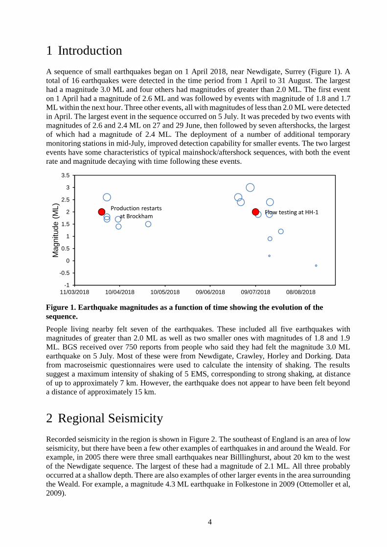
A sequence of small earthquakes began on 1 April 2018, near Newdigate, Surrey (Figure 1). A
total of 16 earthquakes were detected in the time period from 1 April to 31 August. The largest
had a magnitude 3.0 ML and four others had magnitudes of greater than 2.0 ML. The first event
on 1 April had a magnitude of 2.6 ML and was followed by events with magnitude of 1.8 and 1.7
ML within the next hour. Three other events, all with magnitudes of less than 2.0 ML were detected
in April. The largest event in the sequence occurred on 5 July. It was preceded by two events with
magnitudes of 2.6 and 2.4 ML on 27 and 29 June, then followed by seven aftershocks, the largest
of which had a magnitude of 2.4 ML. The deployment of a number of additional temporary
monitoring stations in mid-July, improved detection capability for smaller events. The two largest
events have some characteristics of typical mainshock/aftershock sequences, with both the event
rate and magnitude decaying with time following these events.
People living nearby felt seven of the earthquakes. These included all five earthquakes with
magnitudes of greater than 2.0 ML as well as two smaller ones with magnitudes of 1.8 and 1.9
ML. BGS received over 750 reports from people who said they had felt the magnitude 3.0 ML
earthquake on 5 July. Most of these were from Newdigate, Crawley, Horley and Dorking. Data
from macroseismic questionnaires were used to calculate the intensity of shaking. The results
suggest a maximum intensity of shaking of 5 EMS, corresponding to strong shaking, at distance
of up to approximately 7 km. However, the earthquake does not appear to have been felt beyond
a distance of approximately 15 km.
2 Regional Seismicity
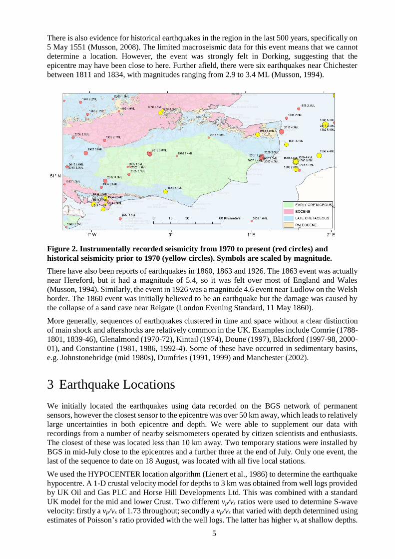
Recorded seismicity in the region is shown in Figure 2. The southeast of England is an area of low
seismicity, but there have been a few other examples of earthquakes in and around the Weald. For
example, in 2005 there were three small earthquakes near Billlinghurst, about 20 km to the west
of the Newdigate sequence. The largest of these had a magnitude of 2.1 ML. All three probably
occurred at a shallow depth. There are also examples of other larger events in the area surrounding
the Weald. For example, a magnitude 4.3 ML earthquake in Folkestone in 2009 (Ottemoller et al,
2009).
Figure 1. Earthquake magnitudes as a function of time showing the evolution of the
sequence.
Production restarts at Brockham
Flow testing at HH-1
-1
-0.5
0
0.5
1
1.5
2
2.5
3
3.5
11/03/2018 10/04/2018 10/05/2018 09/06/2018 09/07/2018 08/08/2018
Magnitude (
ML)
5
There is also evidence for historical earthquakes in the region in the last 500 years, specifically on
5 May 1551 (Musson, 2008). The limited macroseismic data for this event means that we cannot
determine a location. However, the event was strongly felt in Dorking, suggesting that the
epicentre may have been close to here. Further afield, there were six earthquakes near Chichester
between 1811 and 1834, with magnitudes ranging from 2.9 to 3.4 ML (Musson, 1994).
There have also been reports of earthquakes in 1860, 1863 and 1926. The 1863 event was actually
near Hereford, but it had a magnitude of 5.4, so it was felt over most of England and Wales
(Musson, 1994). Similarly, the event in 1926 was a magnitude 4.6 event near Ludlow on the Welsh
border. The 1860 event was initially believed to be an earthquake but the damage was caused by
the collapse of a sand cave near Reigate (London Evening Standard, 11 May 1860).
More generally, sequences of earthquakes clustered in time and space without a clear distinction
of main shock and aftershocks are relatively common in the UK. Examples include Comrie (1788-
1801, 1839-46), Glenalmond (1970-72), Kintail (1974), Doune (1997), Blackford (1997-98, 2000-
01), and Constantine (1981, 1986, 1992-4). Some of these have occurred in sedimentary basins,
e.g. Johnstonebridge (mid 1980s), Dumfries (1991, 1999) and Manchester (2002).
3 Earthquake Locations
We initially located the earthquakes using data recorded on the BGS network of permanent
sensors, however the closest sensor to the epicentre was over 50 km away, which leads to relatively
large uncertainties in both epicentre and depth. We were able to supplement our data with
recordings from a number of nearby seismometers operated by citizen scientists and enthusiasts.
The closest of these was located less than 10 km away. Two temporary stations were installed by
BGS in mid-July close to the epicentres and a further three at the end of July. Only one event, the
last of the sequence to date on 18 August, was located with all five local stations.
We used the HYPOCENTER location algorithm (Lienert et al., 1986) to determine the earthquake
hypocentre. A 1-D crustal velocity model for depths to 3 km was obtained from well logs provided
by UK Oil and Gas PLC and Horse Hill Developments Ltd. This was combined with a standard
UK model for the mid and lower Crust. Two different vp/vs ratios were used to determine S-wave
velocity: firstly a vp/vs of 1.73 throughout; secondly a vp/vs that varied with depth determined using
estimates of Poisson’s ratio provided with the well logs. The latter has higher vs at shallow depths.
Figure 2. Instrumentally recorded seismicity from 1970 to present (red circles) and
historical seismicity prior to 1970 (yellow circles). Symbols are scaled by magnitude.
6
The models are listed in Table 1 and Table 2. A distance weighting scheme, in which weights were
linearly decreased from 1 to 0 between distances of 50 to 250 km, was used to reduce the effect of
lateral heterogeneity in the velocity model for distant stations.
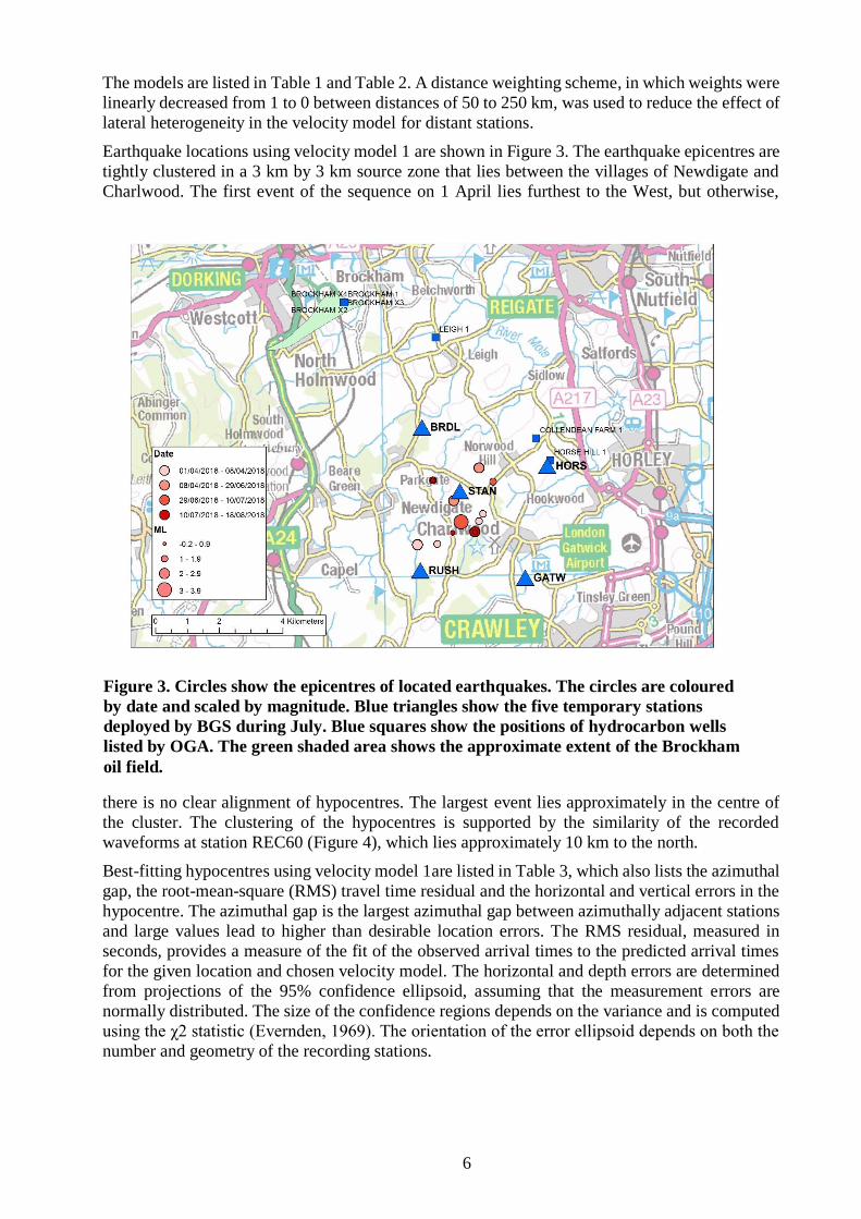
Earthquake locations using velocity model 1 are shown in Figure 3. The earthquake epicentres are
tightly clustered in a 3 km by 3 km source zone that lies between the villages of Newdigate and
Charlwood. The first event of the sequence on 1 April lies furthest to the West, but otherwise,
there is no clear alignment of hypocentres. The largest event lies approximately in the centre of
the cluster. The clustering of the hypocentres is supported by the similarity of the recorded
waveforms at station REC60 (Figure 4), which lies approximately 10 km to the north.
Best-fitting hypocentres using velocity model 1are listed in Table 3, which also lists the azimuthal
gap, the root-mean-square (RMS) travel time residual and the horizontal and vertical errors in the
hypocentre. The azimuthal gap is the largest azimuthal gap between azimuthally adjacent stations
and large values lead to higher than desirable location errors. The RMS residual, measured in
seconds, provides a measure of the fit of the observed arrival times to the predicted arrival times
for the given location and chosen velocity model. The horizontal and depth errors are determined
from projections of the 95% confidence ellipsoid, assuming that the measurement errors are
normally distributed. The size of the confidence regions depends on the variance and is computed
using the χ2 statistic (Evernden, 1969). The orientation of the error ellipsoid depends on both the
number and geometry of the recording stations.
Figure 3. Circles show the epicentres of located earthquakes. The circles are coloured
by date and scaled by magnitude. Blue triangles show the five temporary stations
deployed by BGS during July. Blue squares show the positions of hydrocarbon wells
listed by OGA. The green shaded area shows the approximate extent of the Brockham
oil field.
7
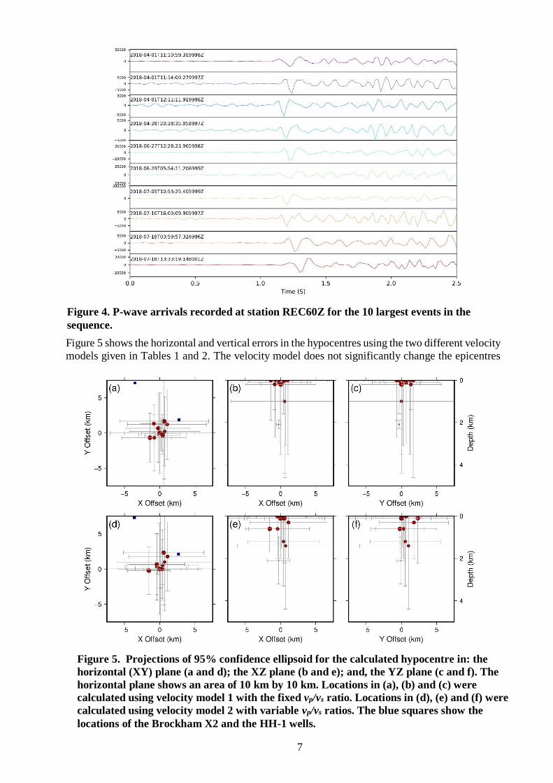
Figure 5 shows the horizontal and vertical errors in the hypocentres using the two different velocity
models given in Tables 1 and 2. The velocity model does not significantly change the epicentres
Figure 4. P-wave arrivals recorded at station REC60Z for the 10 largest events in the
sequence.
Figure 5. Projections of 95% confidence ellipsoid for the calculated hypocentre in: the
horizontal (XY) plane (a and d); the XZ plane (b and e); and, the YZ plane (c and f). The
horizontal plane shows an area of 10 km by 10 km. Locations in (a), (b) and (c) were
calculated using velocity model 1 with the fixed vp/vs ratio. Locations in (d), (e) and (f) were
calculated using velocity model 2 with variable vp/vs ratios. The blue squares show the
locations of the Brockham X2 and the HH-1 wells.

8
or the size of the errors. Using a variable vp/vs ratio results in slightly greater hypocentral depths
for some events, but also increases the RMS residual for all events (Appendix 1).
Regardless of velocity model, the calculated hypocentres for all events except the last in the
sequence generally have depths of less than 1 km. However, the uncertainties in these depths is
relatively large, greater than 1 km in most cases, even using the two local stations installed in early
July. The event on 18 August has a depth of 2.1±0.2 km and was located using all five local
stations. As a result, it has the best constrained depth of all events in the sequence and this depth
may provide a better indicator of the depth of the other events.
4 Resolving Earthquake Depths
We attempt to better resolve earthquake depth by only considering arrival times from stations at
distances of less than 10 km. This means limiting this analysis to the four earthquakes that occurred
on 18 July and were recorded on three local stations and the event on 18 August that was recorded
on five local stations.
We relocated these events using NonLinLoc, a probabilistic, non-linear, global-search earthquake
location algorithm (Lomax et al., 2009). Such nonlinear methods solve the earthquake location
problem by sampling the full solution space. They have the advantage of obtaining a more
complete solution with uncertainties as compared to linearized methods and do not rely on the
quality of an initial estimate of the hypocentre.
Figure 6 shows probability distribution functions (PDFs) of the location of the earthquake on 18
August shown as coloured confidence levels. Results for the two different velocity models are
Figure 6. PDFs for the location of the earthquake on 18 August shown as coloured
confidence levels. The maximum likelihood location is shown as a star. The
Gaussian/Normal expectation is shown as an ellipsoid. The left hand column shows the
confidence regions for velocity model 1. The right hand column shows the confidence
regions for velocity model 2. The top and bottom rows show the horizontal and vertical
planes respectively. Red triangles show the positions of the stations.
9
shown in the left and right hand columns. Again, this demonstrates the relatively high uncertainty
in the estimated depth. The maximum likelihood depths for each model are 1.9 km and 1.8 km.
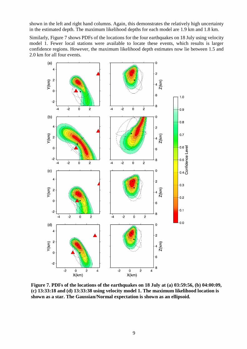
Similarly, Figure 7 shows PDFs of the locations for the four earthquakes on 18 July using velocity
model 1. Fewer local stations were available to locate these events, which results is larger
confidence regions. However, the maximum likelihood depth estimates now lie between 1.5 and
2.0 km for all four events.
Figure 7. PDFs of the locations of the earthquakes on 18 July at (a) 03:59:56, (b) 04:00:09,
(c) 13:33:18 and (d) 13:33:38 using velocity model 1. The maximum likelihood location is
shown as a star. The Gaussian/Normal expectation is shown as an ellipsoid.

10
5 Focal Mechanism
A focal mechanism for the earthquake was determined from measured first motion polarities on
the vertical component of ground velocity seismograms and SH/P amplitude ratios using HASH
(Hardebeck and Shearer, 2003). HASH uses both polarities and SH/P amplitude ratios. Velocity
model 1 and the best fitting hypocentre were used to determine take-off angles. We measured 4
first motion polarities and 4 SH/P amplitude ratios. We also used a grid spacing of 2° for HASH
along with a maximum average error in the amplitude ratio of 0.1. The source mechanisms is
shown in Figure 8. This shows a near vertical, strike slip fault, with either right-lateral slip on a
fault that strikes approximately ENE or left-lateral slip on a fault that strikes approximately NNW.
6 Discussion
Following the earthquakes, there was a great deal of public concern that the Newdigate earthquake
sequence may have been triggered by nearby hydrocarbon exploration and production. Davis and
Frohlich (1993) used a number of criteria to assess whether fluid injection may have induced an
earthquake. Strictly speaking, these are only applicable for seismicity induced by fluid injection.
Figure 8. Lower hemisphere, equal projection of the focal mechanism for the earthquake
on 18 August 2018. The mechanism shows strike slip faulting on a near vertical fault plane
that strikes either NNW or ENE. The white circles and triangles show measured
compressional and dilatational first motions, respectively. Crosses show stations where
SH/P amplitude ratios were measured. The black and white squares show the orientations
of the axes of maximum (P) and minimum (T) compression, respectively.

11
However, they can also be used to assess the evidence that the Newdigate earthquake sequence
may have been triggered by fluid injection or extraction.
1. Are these events the first known earthquakes of this character in the region?
Although the southeast of England is an area of low seismicity, there have been a few other
examples of earthquakes in and around the Weald. For example, in 2005 there were three small
earthquakes near Billlinghurst, about 20 km to the west of the Newdigate sequence. Similarly,
there is also evidence of historical seismicity. This means that natural earthquakes can occur in the
region, albeit rarely.
Is there a clear correlation between injection and seismicity?
Oil production at the nearby Brockham field operated by Angus Energy resumed on 23 March
2018 after a two year hiatus. So there is a temporal correlation between the restart of production
and the first seismicity on 1 April. However, production has been going on for several decades
without any recorded seismicity.
Information provided to OGA by the UK Oil and Gas PLC and the Horse Hill operator, Horse Hill
Developments Ltd, states that pumping to increase wellbore pressure to try to get the well to flow
was carried out in HH-1 on 9 July 2018. The earthquake sequence was already underway at this
time. UK Oil and Gas PLC states that no fluids have been injected into the HH-1 well in 2018.
This appears to rule out operations at HH-1 as a possible causative factor for the earthquake
sequence.
Are epicentres near wells (within 5 km)?
All detected earthquakes are further than 5 km from Brockham. Specifically, the largest of the
earthquakes, the magnitude 3.0 ML event on 5 July, was 8 km from Brockham. Rubinstein and
Mahani (2015) state that seismicity can be induced at distances of 10 km or more away from the
injection point and at significantly greater depths than injection. More recent reports have argued
that seismicity may be induced at 20 km or more from the injection point (Keranen et al., 2014).
However, these examples all involved very large volumes of injected fluids.
Do some earthquakes occur at or near injection depths?
Production at Brockham is from the Portland sandstone at a depth of approximately 600 m. The
first HH-1 test zone was also in the Portland sandstone interval at around 600 m.
Hypocentral depth estimates are generally shallow, though with relatively large uncertainties. The
best constrained event has a depth of 2.1 km and this may be indicative of depths for the rest of
the sequence. This is supported by the fact that using only local stations to locate the events on 18
July gives depths of around 2 km.
Are there known geologic structures that may channel flow to sites of earthquakes?
A number of east-west striking faults that have been mapped between Brockham and the locus of
the earthquakes. These may act as a permeability barrier preventing a direct hydrological
connection and limiting pore pressure increases on the faults to the south. However, increases or
decreases in mass or volume can still cause stress changes at distance that are transmitted
poroelastically (e.g. Segall and Lu, 2015).
Are changes in fluid pressures at well bottoms sufficient to encourage seismicity?
Figures that were provided to OGA give the total volume of fluid extracted at the Brockham field
as 27 m3 in March, 90 m3 in April, 54 m3 in May, 26 m3 in June and 93 m3 in July. This is about
5.5 m3/day on average. Produced water was reinjected into the reservoir (the Portland sandstone)
at a depth of 600 m. Re-injected volumes were 25 m3, 73 m3, 39 m3, 21 m3 and 80 m3 in March,
April, May, June and July approximately 4.5 m3/day on average, giving a net extraction rate of
approximately 1 m3/day. When the first earthquake occurred on 1 April 27 m3 had been extracted,
with 25 m3 re-injected.
12
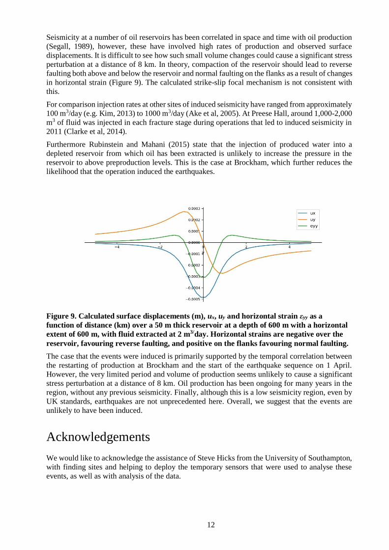
Seismicity at a number of oil reservoirs has been correlated in space and time with oil production
(Segall, 1989), however, these have involved high rates of production and observed surface
displacements. It is difficult to see how such small volume changes could cause a significant stress
perturbation at a distance of 8 km. In theory, compaction of the reservoir should lead to reverse
faulting both above and below the reservoir and normal faulting on the flanks as a result of changes
in horizontal strain (Figure 9). The calculated strike-slip focal mechanism is not consistent with
this.
For comparison injection rates at other sites of induced seismicity have ranged from approximately
100 m3/day (e.g. Kim, 2013) to 1000 m3/day (Ake et al, 2005). At Preese Hall, around 1,000-2,000
m3 of fluid was injected in each fracture stage during operations that led to induced seismicity in
2011 (Clarke et al, 2014).
Furthermore Rubinstein and Mahani (2015) state that the injection of produced water into a
depleted reservoir from which oil has been extracted is unlikely to increase the pressure in the
reservoir to above preproduction levels. This is the case at Brockham, which further reduces the
likelihood that the operation induced the earthquakes.
The case that the events were induced is primarily supported by the temporal correlation between
the restarting of production at Brockham and the start of the earthquake sequence on 1 April.
However, the very limited period and volume of production seems unlikely to cause a significant
stress perturbation at a distance of 8 km. Oil production has been ongoing for many years in the
region, without any previous seismicity. Finally, although this is a low seismicity region, even by
UK standards, earthquakes are not unprecedented here. Overall, we suggest that the events are
unlikely to have been induced.
Acknowledgements
We would like to acknowledge the assistance of Steve Hicks from the University of Southampton,
with finding sites and helping to deploy the temporary sensors that were used to analyse these
events, as well as with analysis of the data.
Figure 9. Calculated surface displacements (m), ux, uy and horizontal strain εyy as a
function of distance (km) over a 50 m thick reservoir at a depth of 600 m with a horizontal
extent of 600 m, with fluid extracted at 2 m3/day. Horizontal strains are negative over the
reservoir, favouring reverse faulting, and positive on the flanks favouring normal faulting.
13
References
AKE, J., MAHRER, K., O’CONNELL, D. AND BLOCK; L., 2005
CLARKE, H., EISNER, L., STYLES, P. ET AL., 2014. Felt seismicity associated with shale gas hydraulic fracturing: the first
documented example in Europe. Geophysical Research Letters, 41: 8308–8314.
DAVIS, S.D. AND FROHLICH, C., 1993. Did (or will) fluid injection cause earthquakes? Criteria for a rational assessment.
Seismological Research Letters 64: 207–224.
EVERNDEN, J.F., 1969. Precision of epicenters obtained by small numbers of world-wide stations. Bulletin of the Seismological
Society of America, 59, 1365–1398.
GRIGOLI, F. ET AL. 2017. Current challenges in monitoring, discrimination, and management of induced seismicity related to
underground industrial activities: A European perspective, Rev. Geophys., 55, 310–340.
HARDEBECK, J. L. AND SHEARER, P. M., 2003. Using S/P Amplitude Ratios to Constrain the Focal Mechanisms of Small
Earthquakes. Bulletin of the Seismological Society of America, 93:2434-2444.
KERANEN, K.M., WEINGARTEN, M., ABERS, G.A., BEKINS, B.A. AND GE, S., 2014. Sharp increase in central Oklahoma seismicity
since 2008 induced by massive wastewater injection. Science, 345, 6195, 448-451
KIM, W.‐Y., 2013. Induced seismicity associated with fluid injection into a deep well in Youngstown, Ohio. Journal of
Geophysical Research, 118, 3506–3518.
LIENERT, B. R. E., BERG, E., AND FRAZER, L. N., 1986. HYPOCENTER: An earthquake location method using centered, scaled, and
adaptively least squares. Bulletin of the Seismological Society of America, 76:771-783.
LOMAX, A., MICHELINI, A. AND CURTIS, A., 2009. Earthquake location, direct, global-search methods. In Encyclopaedia of
Complexity and Systems Science, Part 5. Springer, New York, pp. 2449–2473.
MUSSON, R.M.W., 1994. A catalogue of British earthquakes. British Geological Survey Global Seismology Report, WL/94/04.
Musson, R.M.W., 2008. The seismicity of the British Isles to 1600. British Geological Survey Open Report, OR/08/049.
OTTEMÖLLER, L., BAPTIE, B. AND SMITH, N., 2009. Source Parameters for the 28 April 2007 MW 4.0 Earthquake in Folkestone,
United Kingdom. Bulletin of the Seismological Society of America, 99, 1853–1867.
RUBINSTEIN, J.L. AND MAHANI, A.B. 2015. Myths and Facts on Wastewater Injection, Hydraulic Fracturing, Enhanced Oil
Recovery, and Induced Seismicity. Seismological Research Letters, 86 (4), 1060–1067.
SEGALL, P. 1989. Earthquakes triggered by fluid extraction. Geology, 17, 942-946.
SEGALL, P. AND LU, S. 2015. Injection-induced seismicity: poroelastic and earthquake nucleation effects. Journal of Geophysical
Research, 120, 5082-5103.

14
Tables
Depth Vp Vs Vp/Vs
0 2.2 0.92 1.73
0.2 2.4 1.03 1.73
0.4 2.6 1.15 1.73
0.7 2.7 1.23 1.73
1.2 3.1 1.63 1.73
1.5 3.6 2 1.73
1.8 4.7 2.61 1.73
2.1 5 2.78 1.73
2.4 5.5 3.33 1.73
7.6 6.4 3.7 1.73
18.9 7 4.05 1.73
34.2 8 4.52 1.73
Table 1. Velocity model 1 constructed from the HH-1 well log provided by UKOG Ltd. vs
was calculated using a fixed vp/vs ratio of 1.73 throughout.
Depth Vp Vs Vp/Vs
0 2.2 0.92 2.4
0.2 2.4 1.03 2.33
0.4 2.6 1.15 2.26
0.7 2.7 1.23 2.2
1.2 3.1 1.63 1.9
1.5 3.6 2 1.8
1.8 4.7 2.61 1.8
2.1 5 2.78 1.8
2.4 5.5 3.33 1.65
7.6 6.4 3.7 1.73
18.9 7 4.05 1.73
34.2 8 4.52 1.77
Table 2. Velocity model 2 constructed from the HH-1 well log provided by UKOG Ltd. vs
was calculated using estimates of Poisson’s ratio provided with the well logs. This results in
a vp/vs ratio that varies with depth.
Date Time Latitude Longitude Depth ML NSTA Gap ERY ERX ERZ
01/04/2018 11:10:59 51.155 -0.269 0 2.6 18 158 3.5 3.1 1.9
01/04/2018 11:14:00 51.155 -0.26 0 1.8 10 158 4.7 4.6 2.7
01/04/2018 12:11:11 51.163 -0.239 0 1.7 8 155 4.9 5 3.1
08/04/2018 21:39:56 50.69 -0.145 1 1.7 7 246 93.4 9.1 22.4
28/04/2018 20:38:35 51.161 -0.241 1 1.5 10 156 7.8 7.6 3.4
27/06/2018 12:28:23 51.176 -0.24 0 2.6 14 153 8.2 6.3 4.6
29/06/2018 05:54:11 51.167 -0.252 0.1 2.4 13 155 4.8 4.5 2.9
15
05/07/2018 10:53:23 51.161 -0.249 0.2 3 23 156 5.7 5 3.3
10/07/2018 16:03:10 51.172 -0.234 0 1.9 9 153 5 5.6 3.5
18/07/2018 03:59:55 51.173 -0.261 0.2 1.9 11 93 1.2 1.3 1.9
18/07/2018 04:00:09 51.173 -0.261 0.2 0.2 2 187 2.2 2.8 1.9
18/07/2018 13:33:18 51.158 -0.243 0 2.4 15 107 2.2 2.5 1.6
18/07/2018 13:33:38 51.158 -0.243 0 0.9 3 183 2.8 3.4 1.6
18/08/2018 03:21:58 51.158 -0.253 2.1 -0.2 5 121 0.1 0.3 0.2
Table 3. Earthquake hypocentre parameters determined using the HYPOCENTER
location algorithm and velocity model 1. NSTA is the number of stations used to determine
the location. Gap is the azimuthal gap, the largest azimuthal gap between azimuthally
adjacent stations. RMS is the root-mean-square travel time residual. ERX, ERY and ERZ
are the errors in longitude, latitude and depth (km).
Appendix 1
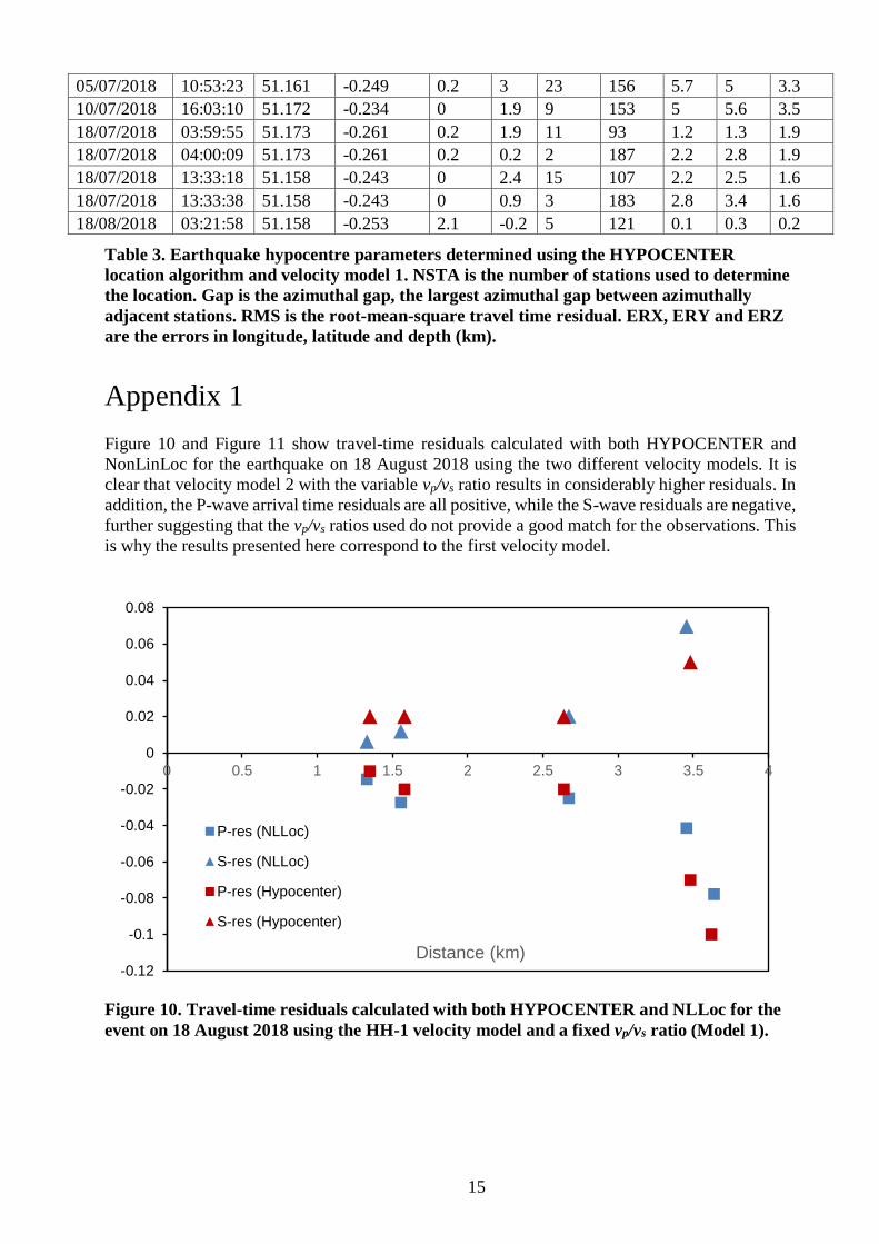
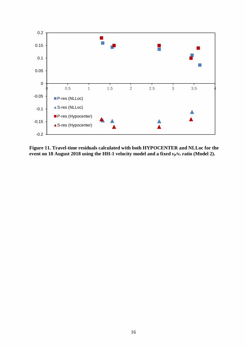
Figure 10 and Figure 11 show travel-time residuals calculated with both HYPOCENTER and
NonLinLoc for the earthquake on 18 August 2018 using the two different velocity models. It is
clear that velocity model 2 with the variable vp/vs ratio results in considerably higher residuals. In
addition, the P-wave arrival time residuals are all positive, while the S-wave residuals are negative,
further suggesting that the vp/vs ratios used do not provide a good match for the observations. This
is why the results presented here correspond to the first velocity model.
-0.12
-0.1
-0.08
-0.06
-0.04
-0.02
0
0.02
0.04
0.06
0.08
0 0.5 1 1.5 2 2.5 3 3.5 4
Distance (km)
P-res (NLLoc)
S-res (NLLoc)
P-res (Hypocenter)
S-res (Hypocenter)
Figure 10. Travel-time residuals calculated with both HYPOCENTER and NLLoc for the
event on 18 August 2018 using the HH-1 velocity model and a fixed vp/vs ratio (Model 1).
16
-0.2
-0.15
-0.1
-0.05
0
0.05
0.1
0.15
0.2
0 0.5 1 1.5 2 2.5 3 3.5 4
P-res (NLLoc)
S-res (NLLoc)
P-res (Hypocenter)
S-res (Hypocenter)
Figure 11. Travel-time residuals calculated with both HYPOCENTER and NLLoc for the
event on 18 August 2018 using the HH-1 velocity model and a fixed vp/vs ratio (Model 2).


