Linear Algebra and its Applications 420 (2007) 490–507www.elsevier.com/locate/laa
The spectra of a graph obtained from copiesof a generalized Bethe tree �
Oscar Rojo∗,1
Departamento de Matemáticas, Universidad Católica del Norte, Castilla 1280, Antofagasta, Chile
Received 6 April 2006; accepted 11 August 2006
Available online 27 September 2006Submitted by R.A. Brualdi
Abstract
We generalize the concept of a Bethe tree as follows: we say that an unweighted rooted tree is a generalizedBethe tree if in each level the vertices have equal degree. If Bk is a generalized Bethe tree of k levels then
we characterize completely the eigenvalues of the adjacency matrix and Laplacian matrix of a graph B(r)k
obtained from the union of r copies of Bk and the cycle Cr connecting the r vertex roots. Moreover, we giveresults on the multiplicity of the eigenvalues, on the spectral radii and on the algebraic conectivity.© 2006 Elsevier Inc. All rights reserved.
AMS classification: 5C50; 15A48
Keywords: Tree; Bethe tree; Laplacian matrix; Adjacency matrix; Algebraic connectivity
1. Preliminaries
Let G be a simple undirected graph on n vertices. The Laplacian matrix of G is the n × n
matrix L(G) = D(G) − A(G) where A(G) is the adjacency and D(G) is the diagonal matrix ofvertex degrees. It is well known that L(G) is a positive semidefinite matrix and that (0, e) is aneigenpair of L(G) where e is the all ones vector. Fiedler [4] proved that G is a connected graphif and only if the second smallest eigenvalue of L(G) is positive. This eigenvalue is called thealgebraic connectivity of G.
� Work supported by Project Fondecyt 1040218, Chile.∗ Tel.: +56 55 355593; fax: +56 55 355599.
E-mail address: [email protected] This work was conducted while the author was visitor at the Instituto Argentino de la Matemática, Buenos Aires,
Argentina.
0024-3795/$ - see front matter ( 2006 Elsevier Inc. All rights reserved.doi:10.1016/j.laa.2006.08.006

O. Rojo / Linear Algebra and its Applications 420 (2007) 490–507 491
A tree is a connected acyclic graph.A Bethe tree [2] is an unweighted rooted tree of k levels such that the vertex root has degree
d, the vertices in the intermediate levels have degree (d + 1) and the vertices in level k are thependant vertices.
We generalize the notion of a Bethe tree as follows: we say that an unweighted rooted tree Bk
of k levels is a generalized Bethe tree if in each level the vertices have equal degree.Throughout this paper Bk denotes a generalized Bethe tree of k levels with k > 1.In [7, 2005], we found the eigenvalues of the adjacency matrix and Laplacian matrix ofBk . They
are the eigenvalues of leading principal submatrices of two nonnegative symmetric tridiagonalmatrices of order k × k whose entries are given in terms of the vertex degrees.
In [8, 2006], we characterized completely the eigenvalues of the adjacency matrix and Laplacianmatrix of a tree B
(2)k obtained from the union of two copies of Bk and the edge connecting the
two vertex roots. If we agree that the two vertex roots are at level 1 and dk−j+1 denotes thedegree of the vertices in level j , then they are the eigenvalues of leading principal submatricesof nonnegative symmetric tridiagonal matrices of order k × k. The codiagonal entries for thesematrices are
√dj − 1, 2 � j � k, while the diagonal entries are 0, . . . , 0, ±1, in the case of the
adjacency matrix, and d1, d2, . . . , dk−1, dk ± 1, in the case of the Laplacian matrix.Let r be a positive integer greater or equal to 3.In this paper, we search for the eigenvalues of the adjacency matrix and Laplacian matrix of a
graph B(r)k obtained from the union of r copies of Bk and the cycle Cr connecting the r vertex
roots. An example of a such graph is
In this graph, we observe four levels of vertices:3 vertices in the cycle C3, say in level 1, each of them with degree equal to 4,6 vertices in level 2, each of them with degree equal to 4,18 vertices in level 3, each of them with degree equal to 3, and36 pendant vertices in level 4.In general, B(r)
k is a graph of k levels such that in each level the vertices have equal degree.We agree that the vertices of Cr are at level 1. For j = 1, 2, . . . , k, let dk−j+1 and nk−j+1 bethe degree of the vertices and number of them in level j . Thus, dk is the degree of the vertices in

492 O. Rojo / Linear Algebra and its Applications 420 (2007) 490–507
level 1, dk > 2, nk = r , d1 = 1, n1 is the number of pendant vertices, and n = ∑kj=1 nk−j+1 is
the total number of vertices.Moreover
nk−1 = (dk − 2)nk (1)
and
nk−j = (dk−j+1 − 1)nk−j+1, 2 � j � k − 1. (2)
Using the labels 1, 2, 3, . . . , n, in this order, our labeling for the vertices of B(r)k is: Label the
vertices of B(r)k from the level k to the level 1 and, in each level, in a counterclockwise sense.
Below is our labeling for the graph given above.
Example 1
1 3 5 7 9 10 11 12
13
14
15
16
18
17
19
20
21
22
23
2425
26
27
28
29
30
31
32
33
34
35
36
37 38 39 40 41 42
43
44
45
46
47
4849
50
51
52
53
54
55 56
57
5859
60
61
6263
2 4 6 8
We recall some notations that we have already introduced in our previous works [7,8].0 is the all zeros matrix of the appropriate order.Im is the identity matrix of order m × m.mj = nj
nj+1for j = 1, 2, . . . , k − 1.
em is the all ones column vector of dimension m.For j = 1, 2, . . . , k − 1, let Cj be the block diagonal matrix
Cj =
⎡⎢⎢⎢⎣
emj
emj
. . .emj
⎤⎥⎥⎥⎦ (3)

O. Rojo / Linear Algebra and its Applications 420 (2007) 490–507 493
with nj+1 diagonal blocks. Thus, the order of Cj is nj × nj+1.We illustrate these notations with the graph in Example 1. This graph has k = 4 levels and
n1 = 36, n2 = 18, n3 = 6, n4 = r = 3,
d1 = 1, d2 = 3, d3 = 4, d4 = 4,
m1 = n1
n2= 2, m2 = n2
n3= 3, m3 = n3
n4= 2.
The matrices defined in (3) are
C1 = diag
{e2, e2, e2, e2, e2, e2, e2, e2, e2, e2, e2, e2,
e2, e2, e2, e2, e2, e2
},
C2 = diag{e3,e3, e3,e3, e3,e3},C3 = {e2, e2, e2}.
At this point, we introduce the r × r symmetric circulant tridiagonal matrix
Er(α) =
⎡⎢⎢⎢⎢⎢⎢⎢⎢⎢⎢⎣
α 1 0 · · · 0 1
1. . .
. . .. . . 0
0. . .
. . .. . .
. . ....
.... . .
. . .. . .
. . . 0
0. . .
. . .. . . 1
1 0 · · · 0 1 α
⎤⎥⎥⎥⎥⎥⎥⎥⎥⎥⎥⎦
.
Our labeling for the vertices of B(r)k yields to the tridiagonal block matrix
A(B
(r)k
)=
⎡⎢⎢⎢⎢⎢⎢⎢⎢⎢⎣
0 C1
CT1 0 C2
CT2
. . .. . .
. . .. . .
. . .. . .
. . . Ck−1
CTk−1 Er(0)
⎤⎥⎥⎥⎥⎥⎥⎥⎥⎥⎦
(4)
for the adjacency matrix of B(r)k , and to the tridiagonal block matrix
L(B
(r)k
)=
⎡⎢⎢⎢⎢⎢⎢⎢⎢⎢⎣
In1 −C1
−CT1 d2In2 −C2
−CT2 d3In3
. . .. . .
. . .. . .
. . . dk−1Ink−1 −Ck−1
−CTk−1 dkIr − Er(0)
⎤⎥⎥⎥⎥⎥⎥⎥⎥⎥⎦
(5)
for the Laplacian matrix of B(r)k .

494 O. Rojo / Linear Algebra and its Applications 420 (2007) 490–507
Lemma 1. If r = 2s then
det Er(α) = (α + 2)(α − 2)
s−1∏l=1
(α + 2 cos
2πl
r
)2
and if r = 2s + 1 then
det Er(α) = (α + 2)
s∏l=1
(α + 2 cos
2πl
r
)2
.
Proof. These formulae follow from the fact that the spectrum of Er(α) is given by the simpleeigenvalues α + 2, α − 2 and the double eigenvalues α + 2 cos 2πl
r, l = 1, 2, . . . , s − 1, when-
ever r = 2s, and, by the simple eigenvalue α + 2 and the double eigenvalues α + 2 cos 2πlr
,l = 1, 2, . . . , s, whenever r = 2s + 1 [3]. �
Lemma 2. Let
M =
⎡⎢⎢⎢⎢⎢⎢⎢⎢⎢⎣
α1In1 C1
CT1 α2In2 C2
CT2
. . .. . .
. . .. . .
. . .. . . αk−1Ink−1 Ck−1
CTk−1 Er(αk)
⎤⎥⎥⎥⎥⎥⎥⎥⎥⎥⎦
.
Let
β1 = α1
and
βj = αj − nj−1
nj
1
βj−1, j = 2, 3, . . . , k, βj−1 /= 0.
Suppose βj /= 0 for all j = 1, 2, . . . , k − 1. If r = 2s then
det M = βn11 β
n22 · · · βnk−1
k−1 (6)
(βk + 2)(βk − 2)
s−1∏l=1
(βk + 2 cos
2πl
r
)2
and if r = 2s + 1 then
det M = βn11 β
n22 · · · βnk−1
k−1 (7)
(βk + 2)
s∏l=1
(βk + 2 cos
2πl
r
)2
.
Proof. Applying the Gaussian elimination procedure, without row interchanges, to M we obtainthe block upper triangular matrix

O. Rojo / Linear Algebra and its Applications 420 (2007) 490–507 495
⎡⎢⎢⎢⎢⎢⎢⎢⎢⎣
β1In1 C1β2In2 C2
β3In3
. . .
. . .. . .
βk−1Ink−1 Ck−1Er(βk)
⎤⎥⎥⎥⎥⎥⎥⎥⎥⎦
.
Hence
det M = βn11 β
n22 · · · βnk−1
k−1 det Er(βk).
Finally we apply Lemma 1 to obtain that det M is given by (6) whenever r = 2s and by (7)whenever r = 2s + 1. �
2. The spectrum of the Laplacian matrix
Let
� = {1, 2, . . . , k − 1}and
� = {j ∈ � : nj > nj+1}.From (1) and (2), we have that for each j , 1 � j � k − 1, nj+1 divides nj . Hence nj � nj+1and, if j ∈ � − � then nj = nj+1 and thus Cj is the identity matrix of order nj .
The polynomials defined below play an important role in our study concerning the eigenvaluesof L
(B
(r)k
).
Definition 1. Let r = 2s or r = 2s + 1. Let
P0(λ) = 1, P1(λ) = λ − 1,
Pj (λ) = (λ − dj )Pj−1(λ) − nj−1
nj
Pj−2(λ), 2 � j � k (8)
and
Pk,l(λ) =(
λ −(
dk − 2 cos2πl
r
))Pk−1(λ) − nk−1
nk
Pk−2(λ) (9)
for l = 0, 1, . . . , s.
Theorem 1. The characteristic polynomial of L(B
(r)k
)is
det(λI − L
(B
(r)k
))= Pk,0(λ)Pk,s(λ)
s−1∏l=1
P 2k,l(λ)
∏j∈�
Pnj −nj+1j (λ), (10)
whenever r = 2s, and
det(λI − L
(B
(r)k
))= Pk,0(λ)
s∏l=1
P 2k,l(λ)
∏j∈�
Pnj −nj+1j (λ), (11)
whenever r = 2s + 1.

496 O. Rojo / Linear Algebra and its Applications 420 (2007) 490–507
Proof. We first suppose that λ ∈ R is such that Pj (λ) /= 0 for all j = 1, 2, . . . , k − 1. We apply
Lemma 2 to M = λI − L(B
(r)k
). From (5)
λI − L(B
(r)k
)
=
⎡⎢⎢⎢⎢⎢⎢⎢⎢⎢⎣
(λ − 1)In1 C1
CT1 (λ − d2)In2 C2
CT2
. . .. . .
. . .. . .
. . .. . . (λ − dk−1)Ink−1 Ck−1
CTk−1 Er(λ − dk)
⎤⎥⎥⎥⎥⎥⎥⎥⎥⎥⎦
.
We have
β1 = λ − 1 = P1(λ) /= 0
β2 = (λ − d2) − n1
n2
1
β1= (λ − d2) − n1
n2
1
P1(λ),
= (λ − d2)P1(λ) − n1n2
P0(λ)
P1(λ)= P2(λ)
P1(λ)/= 0.
Similarly, for j = 3, . . . , k − 1,
βj = (λ − dj ) − nj−1
nj
1
βj−1= (λ − dj ) − nj−1
nj
Pj−2(λ)
Pj−1(λ)
=(λ − dj )Pj−1(λ) − nj−1
njPj−2(λ)
Pj−1(λ)= Pj (λ)
Pj−1(λ)/= 0
and
βk = (λ − dk) − nk−1
nk
1
βk−1
= (λ − dk) − nk−1
nk
Pk−2(λ)
Pk−1(λ)
= (λ − dk)Pk−1(λ) − nk−1nk
Pk−2(λ)
Pk−1(λ)= Pk(λ)
Pk−1(λ).
Let r = 2s. For l = 0, 1, . . . , s, we have
βk + 2 cos2πl
r= Pk(λ)
Pk−1(λ)+ 2 cos
2πl
r
=(λ −
(dk − 2 cos 2πl
r
))Pk−1(λ) − nk−1
nkPk−2(λ)
Pk−1(λ)
= Pk,l(λ)
Pk−1(λ).

O. Rojo / Linear Algebra and its Applications 420 (2007) 490–507 497
In the next steps, for brevity we omit the variable λ. From (6)
det(λI − L
(B
(r)k
))
= Pn11
Pn22
Pn21
Pn33
Pn32
· · · Pnk−1k−1
Pnk−1k−2
Pk,0
Pk−1
Pk,s
Pk−1
P 2k,1
P 2k−1
P 2k,2
P 2k−1
· · · P 2k,s−1
P 2k−1
= Pn1−n21 P
n2−n32 · · · P nk−1−nk
k−1 Pk,0Pk,sP2k,1 · · · P 2
k,s−1
= Pk,0Pk,s
s−1∏l=1
P 2k,l
∏j∈�
Pnj −nj+1j .
Thus (10) is proved all λ ∈ R such that Pj (λ) /= 0 for j = 1, 2, . . . , k − 1. Now, we considerλ0 ∈ R such that Ps(λ0) = 0 for some 1 � s � k − 1. Since the zeros of any nonzero polynomialare isolated, which is the case for the polynomials Pj , there exists a neighborhood N(λ0) of λ0such that Pj (λ) /= 0 for all λ ∈ N(λ0) − {λ0} and for all j = 1, 2, . . . , k − 1. Hence
det(λI − L
(B
(r)k
))= Pk,0(λ)Pk,s(λ)
s−1∏l=1
P 2k,l(λ)
∏j∈�
Pnj −nj+1j (λ)
for all λ ∈ N(λ0) − {λ0}. By continuity, taking the limit as λ tends to λ0 we obtain
det(λ0I − L
(B
(r)k
))= Pk,0(λ0)Pk,s(λ0)
s−1∏l=1
P 2k,l(λ0)
∏j∈�
Pnj −nj+1j (λ0).
Therefore (10) holds for all λ ∈ R. Let now r = 2s + 1. Using (7) and following the same stepsas above (11) is obtained. �
Corollary 1. The spectrum of L(B
(r)k
)is
σ(L
(B
(r)k
))= (∪j∈�{λ : Pj (λ) = 0}) ∪ (∪s
l=0{λ : Pk,l(λ) = 0}), (12)
whenever r = 2s or r = 2s + 1.
Proof. It is an immediate consequence of Theorem 1. �
Definition 2. Let r = 2s or r = 2s + 1. Let Tk,l be the k × k symmetric tridiagonal matrix givenbelow
Tk,l =
⎡⎢⎢⎢⎢⎢⎢⎣
1√
d2 − 1√d2 − 1 d2
√d3 − 1
√d3 − 1
. . .. . .
. . . dk−1√
dk − 2√dk − 2 dk − 2 cos 2πl
r
⎤⎥⎥⎥⎥⎥⎥⎦
for l = 0, 1, . . . , s.
Lemma 3. For j = 1, 2, 3, . . . , k − 1, let Tj be the j × j leading principal submatrix of Tk,0.
Then

498 O. Rojo / Linear Algebra and its Applications 420 (2007) 490–507
det(λI − Tj ) = Pj (λ), j = 1, 2, . . . , k − 1 (13)
and
det(λI − Tk,l) = Pk,l(λ). (14)
Proof. It is well known [1, p. 229] that if Qj is the characteristic polynomial of the j × j leadingprincipal submatrix of the k × k symmetric tridiagonal matrix⎡
⎢⎢⎢⎢⎢⎢⎢⎢⎢⎣
a1 b1b1 a2 b2
b2. . .
. . .. . .
. . .. . .
. . . ak−1 bk−1bk−1 ak
⎤⎥⎥⎥⎥⎥⎥⎥⎥⎥⎦
,
then
Qj(λ) = (λ − aj )Qj−1(λ) − b2j−1Qj−2(λ), j = 2, 3, . . . , k
with
Q0(λ) = 1 and Q1(λ) = λ − a1.
In our case, a1 = 1, aj = dj for j = 2, 3, , . . . , k − 1 and bj =√
nj
nj+1for j = 1, 2, . . . , k − 2.
For these values, the above recursion formula gives the polynomials Pj (λ), j = 0, 1, 2, . . . , k − 1.
Now, we use (2), to see that√
nj
nj+1= √
dj − 1 for j = 1, 2, . . . , k − 2. Thus (13) is proved. For
the matrix Tk,l, we have ak = dk − 2 cos 2πlr
and bk−1 =√
nk−1nk
. The above recursion gives the
polynomial Pk,l(λ). From (1),√
nk−1nk
= √dk − 2. Hence (14) holds. �
Theorem 2. Let Tj , j = 1, 2, . . . , k − 1, and Tk,l, l = 0, 1, 2, . . . , s, be as above. Then
σ(L
(B
(r)k
))= (∪j∈�σ(Tj )) ∪ (∪s
l=0σ(Tk,l)).
Proof. It is an immediate consequence of (12) and Lemma 3. �
Let ρ(A) be the spectral radius of the matrix A.At this point, it is convenient to recall some well known facts. We collect them in the following
Lemma.
Lemma 4. Fact 1. The eigenvalues of a Hermitian matrix do not decrease if a positive semidefinitematrix is added to it [6, Corollary 4.3.3].
Fact 2. If A is an m × m symmetric tridiagonal matrix with nonzero codiagonal entries thenthe eigenvalues of any (m − 1) × (m − 1) principal submatrix strictly interlace the eigenvaluesof A [5].
Fact 3. If A is an irreducible nonnegative matrix then ρ(A) strictly increases when any entryof A strictly increases [9, Theorem 2.1].
Fact 4. If A is an irreducible nonnegative matrix then ρ(A) is a simple eigenvalue of A [9,
Theorem 2.1].

O. Rojo / Linear Algebra and its Applications 420 (2007) 490–507 499
Theorem 3. For r = 2s or r = 2s + 1, we have(a)
σ (Tj−1) ∩ σ(Tj ) = φ, j = 2, 3, . . . , k − 1
and
σ(Tk−1) ∩ σ(Tk,l) = φ, l = 0, 1, . . . , s.
(b) If 0 � p /= q � s then
σ(Tk,p) ∩ σ(Tk,q) = φ.
(c) For j = 1, 2, . . . , k − 1
det Tj = 1
and, for l = 0, 1, . . . , s,
det Tk,l = 2
(1 − cos
2πl
r
).
In particular,
det Tk,0 = 0,
det Tk,s = 2
(1 − cos
2πs
r
).
(d) For j = 1, 2, . . . , k − 1, ρ(Tj ) is a simple eigenvalue of Tj . For l = 0, 1, . . . , s, ρ(Tk,l)
is a simple eigenvalue of Tk,l and the following strict inequalities hold
ρ(Tk,0) < ρ(Tk,1) < · · · < ρ(Tk,s−1) < ρ(Tk,s). (15)
(e) The largest eigenvalue of Tk,s is the spectral radius of L(B
(r)k
).
(f) The smallest eigenvalue of Tk,1 is the algebraic connectivity of B(r)k .
Proof. (a) It follows from Fact 2 of Lemma 4.(b) Suppose that there exists λ ∈ σ(Tk,p) ∩ σ(Tk,q). From (14)
Pk,p(λ) = Pk,q(λ).
That is
(λ −
(dk − 2 cos
2πp
r
))Pk−1(λ) − nk−1
nk
Pk−2(λ)
=(
λ −(
dk − 2 cos2πq
r
))Pk−1(λ) − nk−1
nk
Pk−2(λ).
From this equality and Pk−1(λ) /= 0, it follows that cos 2πpr
= cos 2πqr
which is a contradictionfor 0 � p /= q � s.
(c) For 1 � j � k − 1, the Gaussian elimination procedure, without row interchanges, reducesTj to the upper triangular matrix

500 O. Rojo / Linear Algebra and its Applications 420 (2007) 490–507
⎡⎢⎢⎢⎢⎢⎢⎢⎢⎣
1√
d2 − 11
√d3 − 1
1. . .. . .
√dk−1 − 1
1√
dj − 11
⎤⎥⎥⎥⎥⎥⎥⎥⎥⎦
.
Then det Tj = 1. Let 0 � l � s. The same procedure applied to Tk,l gives the upper triangularmatrices⎡
⎢⎢⎢⎢⎢⎢⎢⎢⎣
1√
d2 − 11
√d3 − 1. . .
. . .
. . .√
dk−1 − 11
√dk − 2
2 − 2 cos 2πlr
⎤⎥⎥⎥⎥⎥⎥⎥⎥⎦
.
Hence det Tk,l = 2(
1 − cos 2πlr
).
(d) Tj , j = 1, 2, . . . , k − 1, and Tk,l , l = 0, 1, . . . , s, are irreducible nonnegative matrices.Then, from Fact 4 of Lemma 4 their corresponding spectral radius are simple eigenvalues.Moreover
0 < 1 − cos2π
r< 1 − cos
4π
r< · · · < 1 − cos
2π(s − 1)
r< 1 − cos
2πs
r.
We now apply Fact 3 of Lemma 4 to obtain the strict inequalities given in (15).(e) From Fact 2 of Lemma 4, we obtain that any eigenvalue in the set ∪k−1
j=1σ(Tj ) is bounded
above by ρ(Tk−1). This fact also implies that ρ(Tk−1) is strictly less that ρ(Tk,l) for all l. Finallywe use Theorem 2 and inequalities (15) to obtain the desired result.
(f) We have
Tk,l+1 = Tk,l +
⎡⎢⎢⎢⎢⎣
0 · · · · · · 0...
. . ....
... 0 00 · · · 0 −2 cos 2π(l+1)
r+ 2 cos 2πl
r
⎤⎥⎥⎥⎥⎦
for l = 0, 1, . . . , s − 1. Moreover
cos2πl
r− cos
2π(l + 1)
r= 2 sin
π(2l + 1)
rsin
π
r> 0
because r � 3 and 0 < 2l+1r
< 1 for 0 � l � s − 1. Now, we apply Fact 1 of Lemma 4 to obtainthat each eigenvalue of Tk,l+1 is greater or equal to the corresponding eigenvalue of Tk,l for alll = 0, 1, . . . , s − 1. In particular, if λk(Tk,l) denotes the smallest eigenvalue of Tk,l then
λk(Tk,0) < λk(Tk,1) < λk(Tk,2) < · · · < λk(Tk,s).
Observe that the strict inequalities hold because, as we already proved, the matrices Tk,l, l =0, 1, . . . , s, do not have eigenvalues in common. Moreover, we already proved that det Tk,0 = 0.
Then λk(Tk,0) = 0. Since the eigenvalues of each matrix Tj interlace the eigenvalues of Tk,1,

O. Rojo / Linear Algebra and its Applications 420 (2007) 490–507 501
it follows that λk(Tk,1) is the smallest positive eigenvalue of L(B
(r)k
), that is, the algebraic
connectivity of B(r)k . �
The next theorem gives information concerning to the multiplicity of the eigenvalues of B(r)k .
Theorem 4. Let Tj , j = 1, 2, . . . , k − 1, and Tk,l, l = 0, 1, 2, . . . , s, be as above. Then
(a) Each eigenvalue of Tj , j ∈ �, as an eigenvalue of L(B
(r)k
)has a multiplicity greater or
equal to (nj − nj+1).
(b) Each eigenvalue of Tk,l, as an eigenvalue of L(B
(r)k
), has a multiplicity greater or equal
to 2 for l = 1, 2, . . . , s − 1 whenever r = 2s and for l = 1, 2, . . . , s whenever r = 2s + 1.
(c) The spectral radius of L(B
(r)k
)is a simple eigenvalue whenever r = 2s and a double
eigenvalue whenever r = 2s + 1.
(d) The algebraic connectivity of B(r)k is a double eigenvalue of L
(B
(r)k
).
Proof. (a) and (b) are immediate consequence of (10) and (11).(c) We know that ρ
(L
(B
(r)k
)) = ρ(Tk,s). Moreover, ρ(Tk,s) is a simple eigenvalue of Tk,s andstrictly greater than the largest eigenvalue of Tj , for j = 1, 2, . . . , k − 1, and strictly greater thanthe largest eigenvalue of Tk,l , for l = 0, 1, . . . , s − 1. Hence the multiplicity of ρ(Tk,s) as aneigenvalue of L
(B
(r)k
)is given by the exponent of the polynomial Pk,s in (10) whenever r = 2s
or in (11) whenever r = 2s + 1.(d) We have proved that λk(Tk,1), the smallest eigenvalue of Tk,1, is the algebraic connectivity
of B(r)k . We apply Fact 2 of Lemma 4 to conclude that λk(Tk,1) /∈ σ(Tj ) for j = 1, 2, . . . , k − 1.
In addition, λk(Tk,1) /∈ σ(Tk,l) for l /= 1 and λk(Tk,1) is a simple eigenvalue of Tk,1. Therefore,the multiplicity of λk(Tk,1) as an eigenvalue of L
(B
(r)k
)is given by the exponent of the polynomial
Pk,1 in (10) whenever r = 2s or in (11) whenever r = 2s + 1. In both cases this exponent is 2. �
Example 2. For the graph in Example 1 we have
k = 4, r = 3, s = 1, n1 = 36, d1 = 1, n2 = 18, d2 = 3,
n3 = 6, d3 = 4, n4 = 3, d4 = 4 and � = {1, 2, 3}.From Theorem 2, the eigenvalues of L
(B
(3)4
)are the eigenvalues of T1, T2, T3, T4,0 and T4,1:
T1 = [1], T2 =[
1√
2√2 3
], T3 =
⎡⎣ 1
√2√
2 3√
3√3 4
⎤⎦ ,
T4,0 =
⎡⎢⎢⎣
1√
2√2 3
√3√
3 4√
2√2 4 − 2 cos 0
⎤⎥⎥⎦ =
⎡⎢⎢⎣
1√
2√2 3
√3√
3 4√
2√2 2
⎤⎥⎥⎦ ,
T4,1 =
⎡⎢⎢⎣
1√
2√2 3
√3√
3 4√
2√2 4 − 2 cos 2π
3
⎤⎥⎥⎦ =
⎡⎢⎢⎣
1√
2√2 3
√3√
3 4√
2√2 5
⎤⎥⎥⎦ .
502 O. Rojo / Linear Algebra and its Applications 420 (2007) 490–507
To four decimal places these eigenvalues are
multiplicityT1: 1 n1 − n2 = 18T2: 0.2679 3.7321 n2 − n3 = 12T3: 0.0746 2.4481 5.4774 n3 − n4 = 3T4,0: 0 1.2087 3 5.7913 1T4,1: 0.0496 2.1456 4.3968 6.4080 2
Since the matrices T1, T2, T3, T4,0 and T4,1 do not have eigenvalues in common, each eigenvalueof L
(B
(r)k
)has the multiplicity indicated in the last column.
Below we give another example
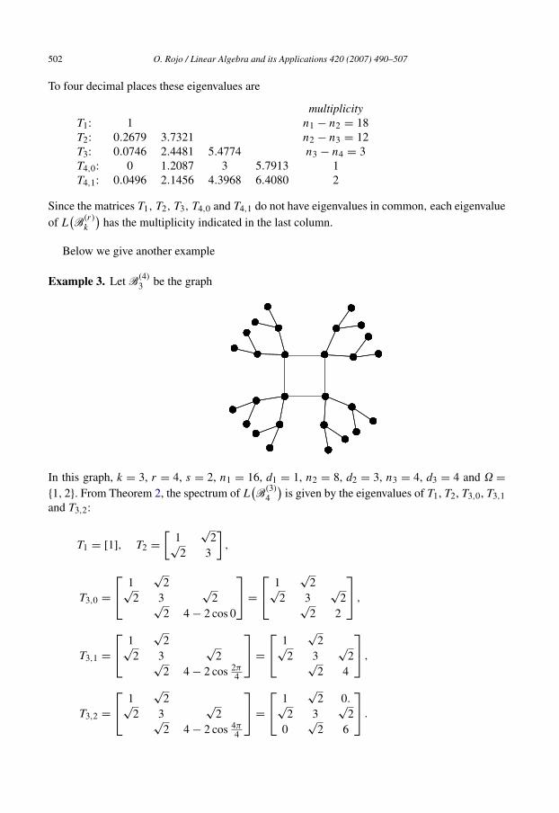
Example 3. Let B(4)3 be the graph
In this graph, k = 3, r = 4, s = 2, n1 = 16, d1 = 1, n2 = 8, d2 = 3, n3 = 4, d3 = 4 and � ={1, 2}. From Theorem 2, the spectrum of L
(B
(3)4
)is given by the eigenvalues of T1, T2, T3,0, T3,1
and T3,2:
T1 = [1], T2 =[
1√
2√2 3
],
T3,0 =⎡⎣ 1
√2√
2 3√
2√2 4 − 2 cos 0
⎤⎦ =
⎡⎣ 1
√2√
2 3√
2√2 2
⎤⎦ ,
T3,1 =⎡⎣ 1
√2√
2 3√
2√2 4 − 2 cos 2π
4
⎤⎦ =
⎡⎣ 1
√2√
2 3√
2√2 4
⎤⎦ ,
T3,2 =⎡⎣ 1
√2√
2 3√
2√2 4 − 2 cos 4π
4
⎤⎦ =
⎡⎣ 1
√2 0.√
2 3√
20
√2 6
⎤⎦ .

O. Rojo / Linear Algebra and its Applications 420 (2007) 490–507 503
The eigenvalues are
multiplicityT1: 1 n1 − n2 = 8T2: 0.2679 3.7321 n2 − n3 = 4T3,0: 0 1.5858 4.4142 1T3,1: 0.1442 2.6784 5.1774 2T3,2: 0.1892 3.1969 6.6139 1
As in Example 2, since the matrices T1, T2, T3,0, T3,2 and T3,2 do not have eigenvalues in common,each eigenvalue of L
(B
(r)k
)has the multiplicity given in the last column.
3. The spectrum of the adjacency matrix
In this section we search for the spectrum of the adjacency matrix of B(r)k .
Let
D =
⎡⎢⎢⎢⎢⎢⎢⎢⎣
−In1
In2 −In3
. . .(−1)k−1Ink−1
(−1)kIr
⎤⎥⎥⎥⎥⎥⎥⎥⎦
.
One can easily see that
D(λI + A
(B
(r)k
))D−1 = λI − A
(B
(r)k
). (16)
Definition 3. Let r = 2s or r = 2s + 1. Let
S0(λ) = 1, S1(λ) = λ,
Sj (λ) = λSj−1(λ) − nj−1
nj
Sj−2(λ), 2 � j � k,
and
Sk,l(λ) =(
λ + 2 cos2πl
r
)Sk−1(λ) − nk−1
nk
Sk−2(λ)
for l = 0, 1, . . . , s.
Theorem 5. The characteristic polynomial of A(B
(r)k
)is
det(λI − A
(B
(r)k
))= Sk,0(λ)Sk,s(λ)
s−1∏l=1
S2k,l(λ)
∏j∈�
Snj −nj+1j (λ), (17)
whenever r = 2s, and
det(λI − A
(B
(r)k
))= Sk,0(λ)
s∏l=1
S2k,l(λ)
∏j∈�
Snj −nj+1j (λ) (18)
whenever r = 2s + 1.

504 O. Rojo / Linear Algebra and its Applications 420 (2007) 490–507
Proof. Similar to the proof of Theorem 1. Apply Lemma 2 to the matrix M = λI + A(B
(r)k
).
For this matrix αj = λ for j = 1, 2, . . . , k. From (16), we have det(λI − A
(B
(r)k
)) = det(λI +
A(B
(r)k
)). This concludes the proof. �
Corollary 2. The spectrum of A(B
(r)k
)is
σ(A
(B
(r)k
))= (∪j∈�{λ : Sj (λ) = 0}) ∪ (∪s
l=0{λ : Sk,l(λ) = 0}) (19)
whenever r = 2s or r = 2s + 1.
Proof. It is an immediate consequence of Theorem 5. �
Definition 4. Let r = 2s or r = 2s + 1. Let Rk,l be the k × k symmetric tridiagonal matrix givenbelow
Rk,l =
⎡⎢⎢⎢⎢⎢⎢⎣
0√
d2 − 1√d2 − 1 0
√d3 − 1
√d3 − 1
. . .. . .
. . . 0√
dk − 2√dk − 2 2 cos 2πl
r
⎤⎥⎥⎥⎥⎥⎥⎦
for l = 0, 1, . . . , s.
Lemma 5. For j = 1, 2, 3, . . . , k − 1, let Rj be the j × j leading principal submatrix of Rk,0Then
det(λI − Rj ) = Sj (λ), j = 1, 2, . . . , k − 1,
and
det(λI − Rk,l) = Sk,l(λ). (20)
Proof. Similar to the proof of Lemma 3. �
Theorem 6. Let Rj , j = 1, 2, . . . , k − 1, and Rk,l, l = 0, 1, 2, . . . , s, be as above. Then
σ(A
(B
(r)k
))= (∪j∈�σ(Rj )) ∪ (∪s
l=0σ(Rk,l)).
Proof. It is an immediate consequence of (19) and Lemma 5. �
Theorem 7. For r = 2s or r = 2s + 1 we have(a)
σ (Rj−1) ∩ σ(Rj ) = φ, j = 2, 3, . . . , k − 1
and
σ(Rk−1) ∩ σ(Rk,l) = φ, l = 0, 1, . . . , s.
(b) If 0 � p /= q � s then
σ(Rk,p) ∩ σ(Rk,q) = φ.

O. Rojo / Linear Algebra and its Applications 420 (2007) 490–507 505
(c) For j = 1, 2, . . . , k − 1, ρ(Rj ) is a simple eigenvalue of Rj . For l = 0, 1, . . . , s, eacheigenvalue of Rk,l is simple.
(d) The largest eigenvalue of Rk,0 is the spectral radius of A(B
(r)k
).
Proof. (a) It follows from Fact 2 of Lemma 4.(b) Suppose that there exists λ ∈ σ(Rk,p) ∩ σ(Rk,q). From (20)
Sk,p(λ) = Sk,q(λ).
That is(λ + 2 cos
2πp
r
)Sk−1(λ) − nk−1
nk
Sk−2(λ)
=(
λ + 2 cos2πq
r
)Sk−1(λ) − nk−1
nk
Sk−2(λ).
From this equality and Sk−1(λ) /= 0, it follows that cos 2πpr
= cos 2πqr
which is a contradictionfor 0 � p /= q � s.
(c) Rj , j = 1, 2, . . . , k − 1, are irreducible nonnegative matrices. Then, from Fact 4 of Lemma4, their corresponding spectral radius are simple eigenvalues. Finally, from Fact 2 of Lemma 4, itfollows that each eigenvalue of Rk,l is simple.
(d) From Fact 2 of Lemma 4, we obtain that any eigenvalue in the set ∪k−1j=1σ(Rj ) is bounded
above by ρ(Rk−1). This fact also implies that ρ(Rk−1) is strictly less than ρ(Rk,l) for all l.Applying Fact 1 of Theorem 4 to
Rk.0 = Rk,l +
⎡⎢⎢⎢⎢⎣
0 · · · · · · 0...
. . ....
... 0 00 · · · 0 2 − 2 cos 2πl
r
⎤⎥⎥⎥⎥⎦ ,
we obtain that the largest eigenvalue of Rk,l , for all l, is less than ρ(Rk,0). Since Rk,0 is anirreducible nonnegative matrix, ρ(Rk,0) is a simple eigenvalue of Rk,0. Finally we use Theorem6 to conclude the proof. �
Theorem 8. Let Rj , j = 1, 2, . . . , k − 1, and Rk,l, l = 0, 1, 2, . . . , s, be as above. Then
(a) Each eigenvalue of Rj , j ∈ �, as an eigenvalue of A(B
(r)k
)has a multiplicity greater or
equal to (nj − nj+1).
(b) Each eigenvalue of Rk,l, as an eigenvalue of A(B
(r)k
), has a multiplicity greater or equal
to 2 for l = 1, 2, . . . , s − 1 whenever r = 2s and for l = 1, 2, . . . , s whenever r = 2s + 1.
(c) The spectral radius of A(B
(r)k
)is a simple eigenvalue.
Proof. (a) and (b) are immediate consequences of (17) and (18).(c) Since A
(B
(r)k
)is an irreducible nonnegative matrix, ρ
(A
(B
(r)k
))is a simple eigenvalue.
�
Example 4. For the graph in Example 1 we have
k = 4, r = 3, s = 1, n1 = 36, d1 = 1, n2 = 18, d2 = 3,
n3 = 6, d3 = 4, n4 = 3, d4 = 4 and � = {1, 2, 3}.

506 O. Rojo / Linear Algebra and its Applications 420 (2007) 490–507
From Theorem 6, the eigenvalues of A(B
(3)4
)are the eigenvalues of R1, R2, R3, R4,0 and R4,1:
R1 = [0], R2 =[
0.√
2√2 0
], R3 =
⎡⎣ 0
√2√
2 0√
3√3 0
⎤⎦ ,
R4,0 =
⎡⎢⎢⎣
0√
2√2 0
√3√
3 0√
2√2 2 cos 0
⎤⎥⎥⎦ =
⎡⎢⎢⎣
0√
2√2 0
√3√
3 0√
2√2 2
⎤⎥⎥⎦ ,
R4,1 =
⎡⎢⎢⎣
0√
2√2 0
√3√
3 0√
2√2 2 cos 2π
3
⎤⎥⎥⎦ =
⎡⎢⎢⎣
0√
2√2 0
√3 0√
3 0√
2√2 −1
⎤⎥⎥⎦ .
The eigenvalues are
multiplicityR1: 0 n1 − n2 = 18R2: −1.4142 1.4142 n2 − n3 = 12R3: −2.2361 0 2.2361 n3 − n4 = 3R4,0: −2.3890 −0.3315 1.6387 3.0818 1R4,1: −2.7029 −1.2287 0.4942 2.4374 2
Since R1, R2, R3, R4,0 and R4,1 do not have eigenvalues in common, except for the eigenvalue 0,each nonzero eigenvalue of the adjacency matrix has the multiplicity indicated in the last column.The eigenvalue 0 has a multiplicity equal to 18 + 3 = 21.
Example 5. For the graph in Example 3, we have k = 3, r = 4, s = 2, n1 = 16, d1 = 1, n2 = 8,d2 = 3, n3 = 4, d3 = 4 and � = {1, 2}. From Theorem 6, the spectrum of A
(B
(3)4
)is given by
the eigenvalues of R1, R2, R3,0, R3,1 and R3,2:
R1 = [0], R2 =[
0√
2√2 0
],
R3,0 =⎡⎣ 0
√2√
2 0√
2√2 2 cos 0
⎤⎦ =
⎡⎣ 0
√2√
2 0√
2√2 2
⎤⎦
R3,1 =⎡⎣ 0
√2√
2 0√
2√2 2 cos 2π
4
⎤⎦ =
⎡⎣ 0
√2√
2 0√
2√2 0
⎤⎦
R3,2 =⎡⎣ 0
√2√
2 0√
2√2 2 cos 4π
4
⎤⎦ =
⎡⎣ 0
√2√
2 0√
2√2 −2
⎤⎦ .

O. Rojo / Linear Algebra and its Applications 420 (2007) 490–507 507
The eigenvalues are
multiplicityR1: 0 n1 − n2 = 8R2: −1.4142 1.4142 n2 − n1 = 4R3,0: −1.7093 0.8061 2.9032 1R3,1: −2 0 2 2R3,2: −2.9032 −0.8061 1.7093 1
As in Example 4, each nonzero eigenvalue of the adjacency matrix has the multiplicity given inthe last column. The multiplicity of the eigenvalue 0 is equal to 8 + 2 = 10.
Acknowledgement
The author is greatful to the referee for valuable comments which led to an improved versionof the paper.
References
[1] L.N. Trefethen, D. Bau III, Numerical Linear Algebra, Society for Industrial and Applied Mathematics, 1997.[2] O.J. Heilmann, E.H. Lieb, Theory of monomer-dimer systems, Comm. Math. Phys. 25 (1972) 190–232.[3] P.J. Davis, Circulant Matrices, John Wiley and Sons, New York, 1979.[4] M. Fiedler, Algebraic connectivity of graphs, Czechoslovak Math. J. 23 (1973) 298–305.[5] G.H. Golub, C.F. Van Loan, Matrix Computations, second ed., Johns Hopkins University Press, Baltimore, 1989.[6] R.A. Horn, C.R. Johnson, Matrix Analysis, Cambridge University Press, Cambridge, 1991.[7] O. Rojo, R. Soto, The spectra of the adjacency matrix and Laplacian matrix for some balanced trees, Linear Algebra
Appl. 403 (2005) 97–117.[8] O. Rojo, The spectra of some trees and bounds for the largest eigenvalue of any tree, Linear Algebra Appl. 414 (2006)
199–217.[9] R.S. Varga, Matrix Iterative Analysis, Prentice-Hall Inc., 1965.


