These slides based almost entirely on a set provided by Prof. Eric Miller
Imaging from Projections
Eric MillerWith minor modifications by
Dana Brooks
These slides based almost entirely on a set provided by Prof. Eric Miller
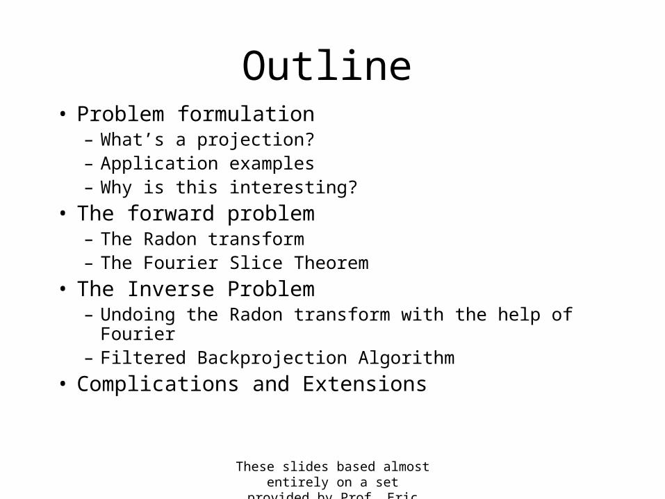
Outline• Problem formulation
– What’s a projection?– Application examples– Why is this interesting?
• The forward problem– The Radon transform – The Fourier Slice Theorem
• The Inverse Problem– Undoing the Radon transform with the help of Fourier– Filtered Backprojection Algorithm
• Complications and Extensions
These slides based almost entirely on a set provided by Prof. Eric Miller
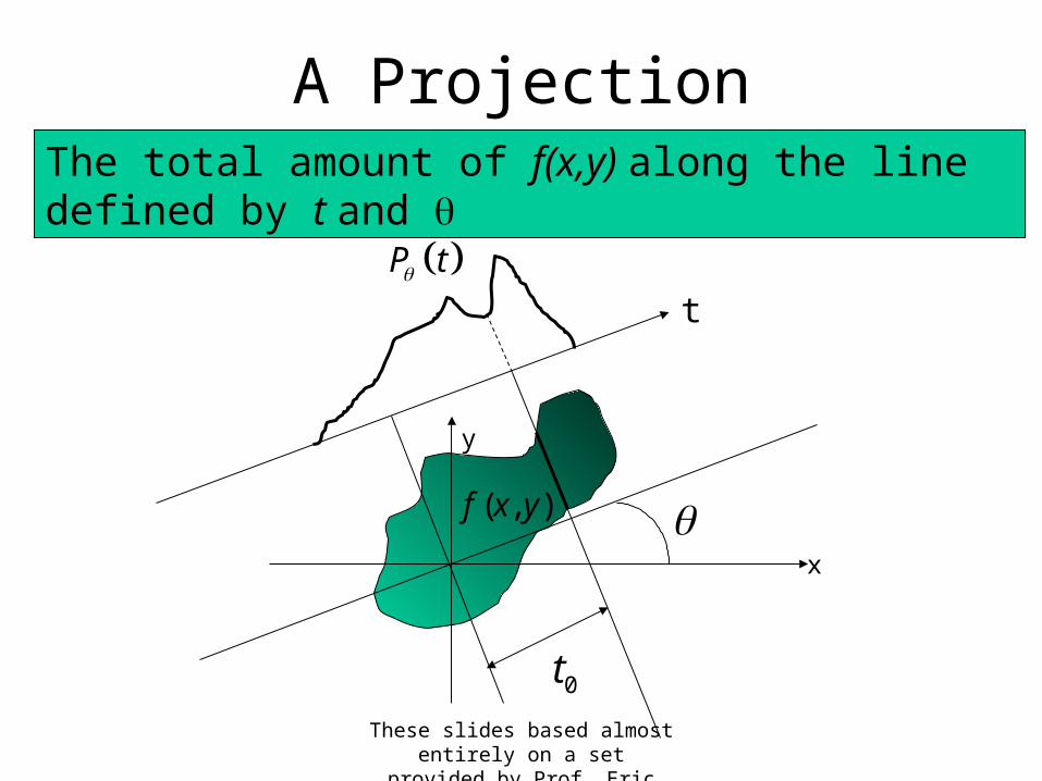
A ProjectionThe total amount of f(x,y) along the line defined by t and
x
y
t
P t
0t
( , )f x y
These slides based almost entirely on a set provided by Prof. Eric Miller
Application Examples• CAT scans:
– X ray source moves around the body– f(x,y) is the density of the tissue
• MRI– Not as clear cut what the “projection” is, but in a peculiar way, the math is
the same (remind me to talk about this when we get to the MRI Imaging equation …)
– f(x,y) is the spin density of molecules in the tissue
• Synthetic Aperture Radar– Satellite moves down a linear track collecting radar echoes of the ground– Used for remote sensing, surveillance, …– Again: math is the same (after much pain and anguish)– f(x,y) is the reflectivity of the earth surface
These slides based almost entirely on a set provided by Prof. Eric Miller
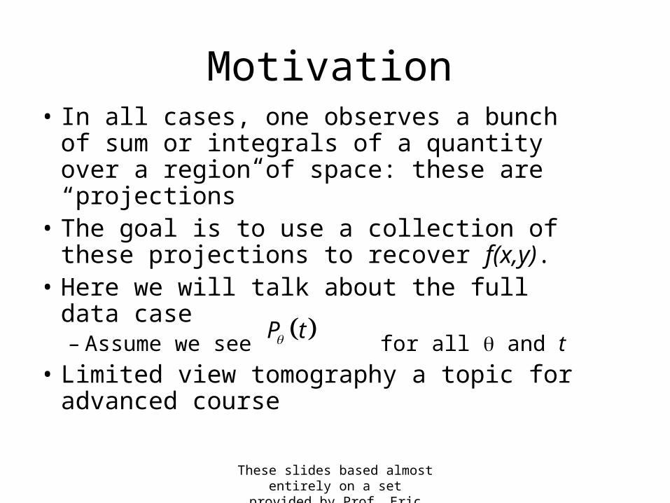
Motivation• In all cases, one observes a bunch of sum or
integrals of a quantity over a region of space: these are “projections”
• The goal is to use a collection of these projections to recover f(x,y).
• Here we will talk about the full data case– Assume we see for all and t
• Limited view tomography a topic for advanced course
P t

These slides based almost entirely on a set provided by Prof. Eric Miller
The Radon Transform
x
y
t
P t
( , )f x y
ds
, line
,
, cos sin
t
P t f x y ds
f x y x y t dxdy
Polar equation for line:cos sinx y t
Function oft and
So the line exists only where this equation is true
These slides based almost entirely on a set provided by Prof. Eric Miller
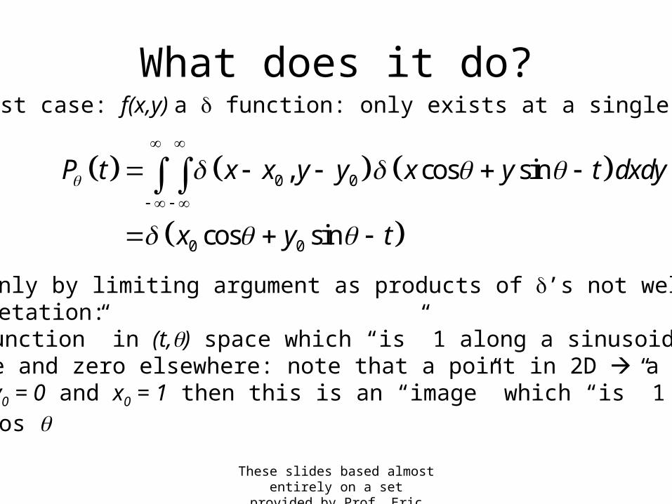
What does it do?Simplest case: f(x,y) a function: only exists at a single point
0 0
0 0
, cos sin
cos sin
P t x x y y x y t dxdy
x y t
• Proof only by limiting argument as products of ’s not well defined• Interpretation:
• A “function” in (t,) space which “is” 1 along a sinusoidal curve and zero elsewhere: note that a point in 2D a curve• Say y0 = 0 and x0 = 1 then this is an “image” which “is” 1 when t = cos
These slides based almost entirely on a set provided by Prof. Eric Miller
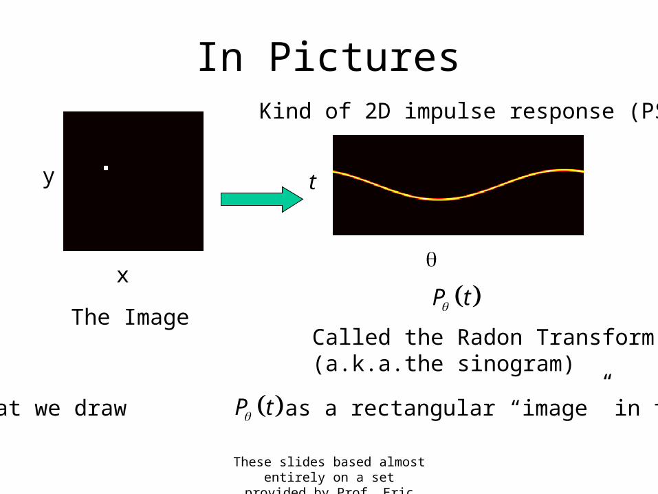
In Pictures
x
y
t
The ImageCalled the Radon Transform(a.k.a.the sinogram)
Kind of 2D impulse response (PSF)
Note that we draw as a rectangular “image” in t and P t
P t
These slides based almost entirely on a set provided by Prof. Eric Miller
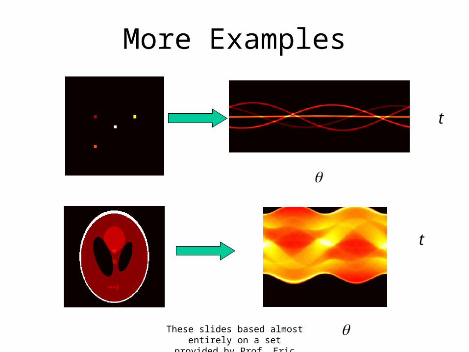
More Examples
t
t
These slides based almost entirely on a set provided by Prof. Eric Miller
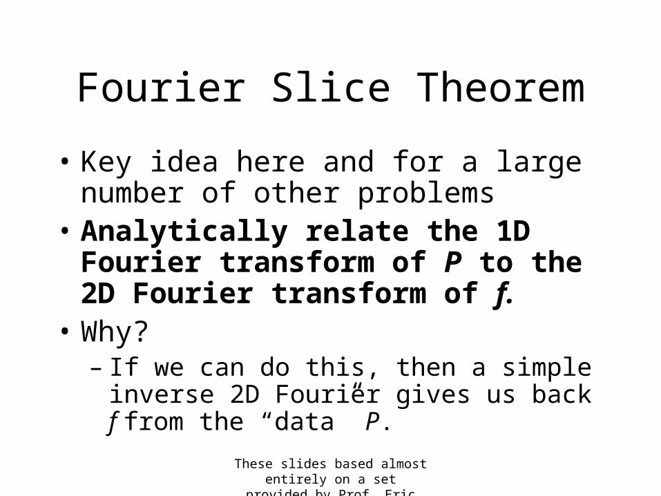
Fourier Slice Theorem
• Key idea here and for a large number of other problems
• Analytically relate the 1D Fourier transform of P to the 2D Fourier transform of f.
• Why?– If we can do this, then a simple inverse 2D
Fourier gives us back f from the “data” P.
These slides based almost entirely on a set provided by Prof. Eric Miller
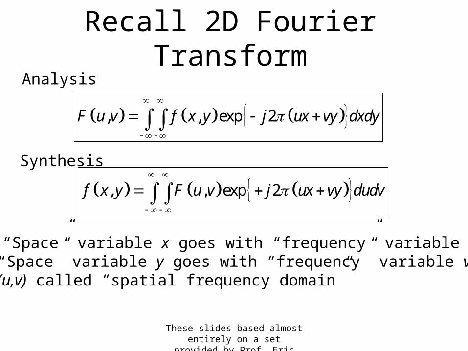
Recall 2D Fourier Transform
, , exp 2F u v f x y j ux vy dxdy
Analysis
Synthesis
, , exp 2f x y F u v j ux vy dudv
• “Space” variable x goes with “frequency” variable u• “Space” variable y goes with “frequency” variable v• (u,v) called “spatial frequency domain”
These slides based almost entirely on a set provided by Prof. Eric Miller
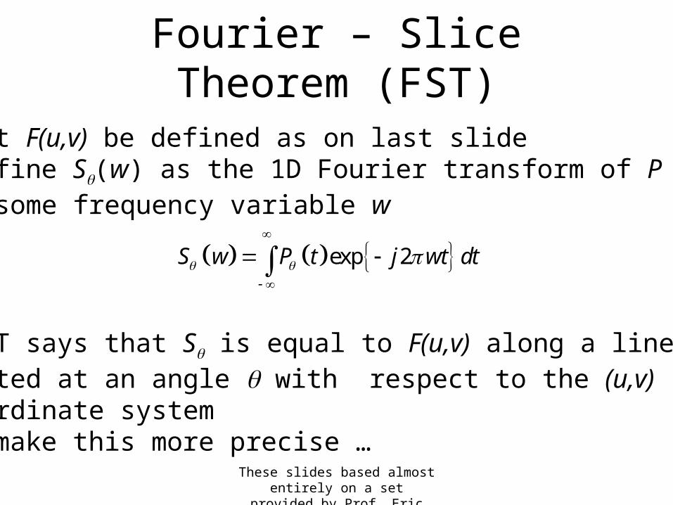
Fourier – Slice Theorem (FST)
• Let F(u,v) be defined as on last slide• Define S(w) as the 1D Fourier transform of P along t for some frequency variable w
• FST says that S is equal to F(u,v) along a line tilted at an angle with respect to the (u,v) coordinate system•To make this more precise …
exp 2S w P t j wt dt
These slides based almost entirely on a set provided by Prof. Eric Miller
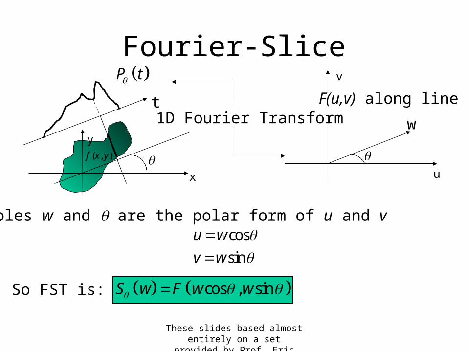
Fourier-Slice
x
y
t
( , )f x y
P t
1D Fourier Transform
u
v
F(u,v) along line
w
Variables w and are the polar form of u and vcos
sin
u w
v w
So FST is: cos , sinS w F w w
These slides based almost entirely on a set provided by Prof. Eric Miller
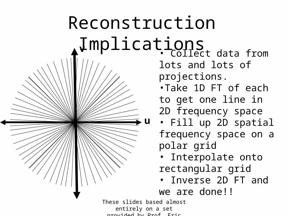
Reconstruction Implications• Collect data from lots and lots of projections.•Take 1D FT of each to get one line in 2D frequency space• Fill up 2D spatial frequency space on a polar grid• Interpolate onto rectangular grid• Inverse 2D FT and we are done!!
u
v
These slides based almost entirely on a set provided by Prof. Eric Miller
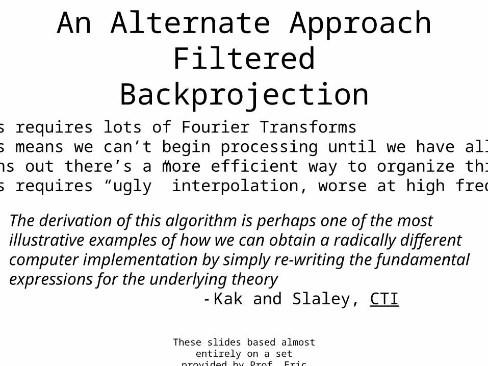
An Alternate ApproachFiltered Backprojection
The derivation of this algorithm is perhaps one of the most illustrative examples of how we can obtain a radically differentcomputer implementation by simply re-writing the fundamentalexpressions for the underlying theory
- Kak and Slaley, CTI
• This requires lots of Fourier Transforms• This means we can’t begin processing until we have all slices• Turns out there’s a more efficient way to organize things• This requires “ugly” interpolation, worse at high frequencies
These slides based almost entirely on a set provided by Prof. Eric Miller
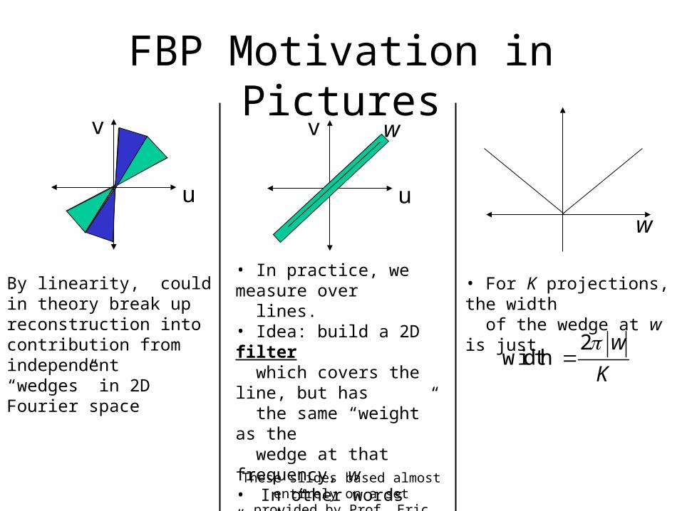
FBP Motivation in Pictures
u
v
By linearity, could in theory break up reconstruction intocontribution from independent“wedges” in 2D Fourier space
u
v
• In practice, we measure over lines. • Idea: build a 2D filter which covers the line, but has the same “weight” as the wedge at that frequency, w• In other words “mush” triangle to a rectangle• Then “sum up” filtered projections
w
• For K projections, the width of the wedge at w is just
2width
w
K
w
These slides based almost entirely on a set provided by Prof. Eric Miller
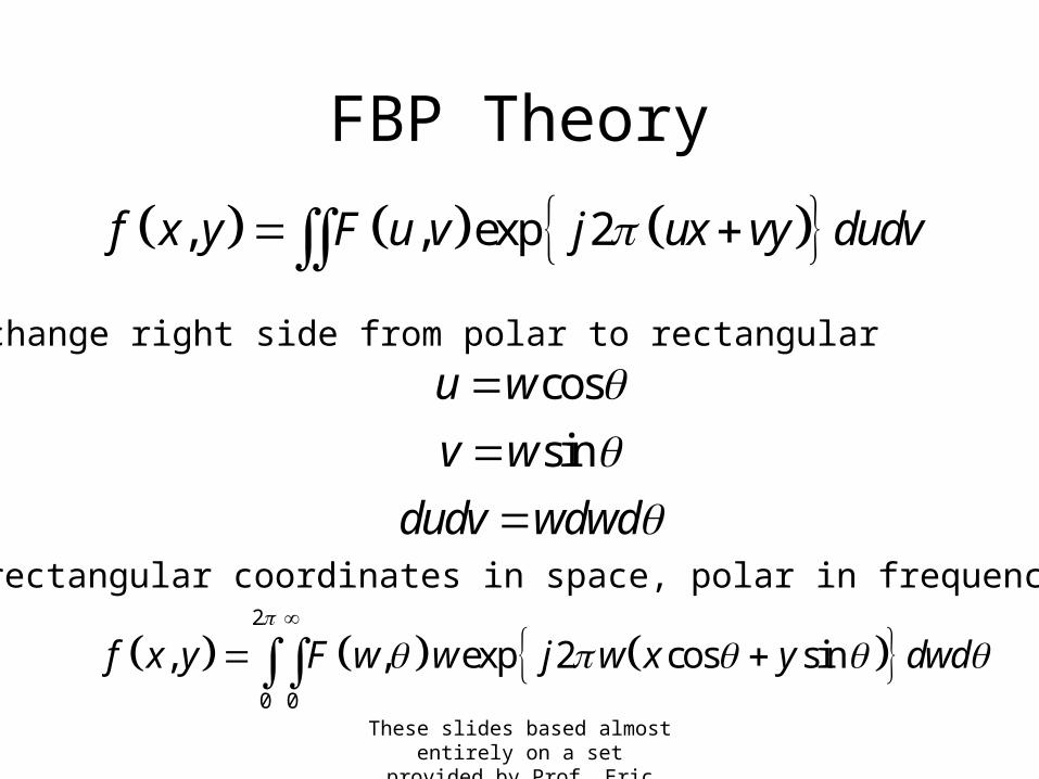
FBP Theory
, , exp 2f x y F u v j ux vy dudv Now, change right side from polar to rectangular
cos
sin
u w
v w
dudv wdwd
To get rectangular coordinates in space, polar in frequency:
2
0 0
, , exp 2 cos sinf x y F w w j w x y dwd
These slides based almost entirely on a set provided by Prof. Eric Miller
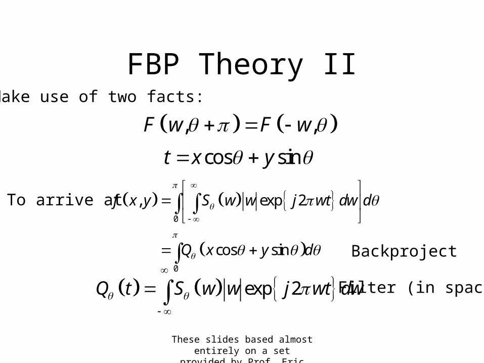
FBP Theory IIMake use of two facts:
, ,
cos sin
F w F w
t x y
To arrive at
0
0
, exp 2
cos sin
f x y S w w j wt dw d
Q x y d
exp 2Q t S w w j wt dw
Filter (in space)
Backproject
These slides based almost entirely on a set provided by Prof. Eric Miller
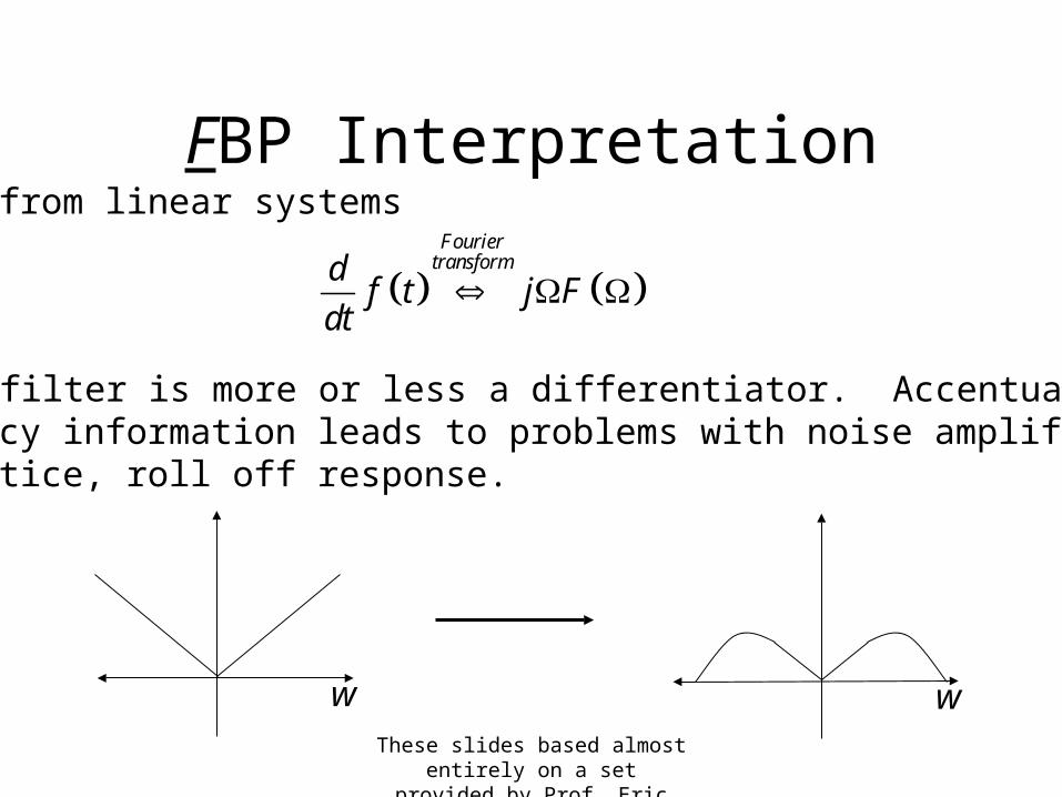
FBP Interpretation• Recall from linear systems
• So |w| filter is more or less a differentiator. Accentuated high frequency information leads to problems with noise amplification• In practice, roll off response.
Fourier
transformdf t j F
dt
w w
These slides based almost entirely on a set provided by Prof. Eric Miller
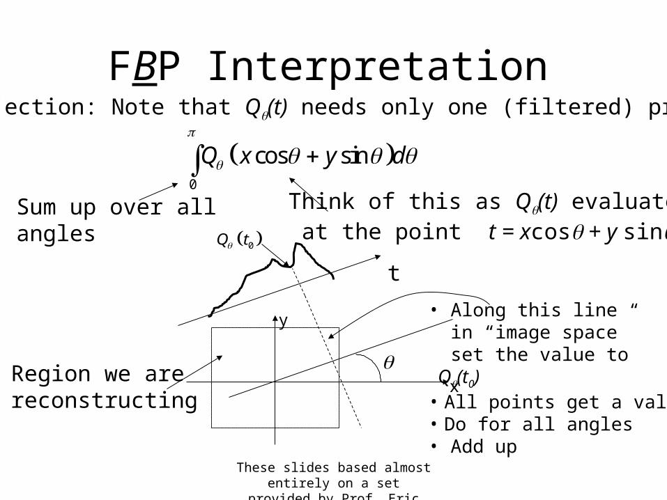
FBP Interpretation
0
cos sinQ x y d
Backprojection: Note that Q(t) needs only one (filtered) projection
Sum up over allangles
Think of this as Q(t) evaluated at the point t = xcos + y sin
x
y
t
0Q t
Region we arereconstructing
• Along this line in “image space” set the value to Q(t0)• All points get a value• Do for all angles• Add up
These slides based almost entirely on a set provided by Prof. Eric Miller
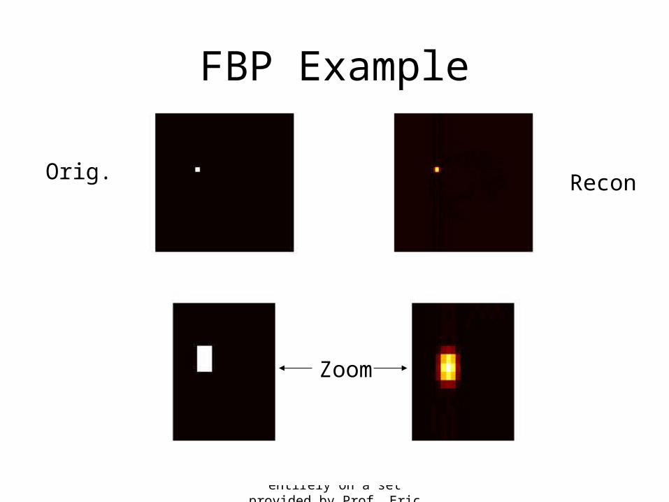
FBP Example
Orig. Recon
Zoom
These slides based almost entirely on a set provided by Prof. Eric Miller
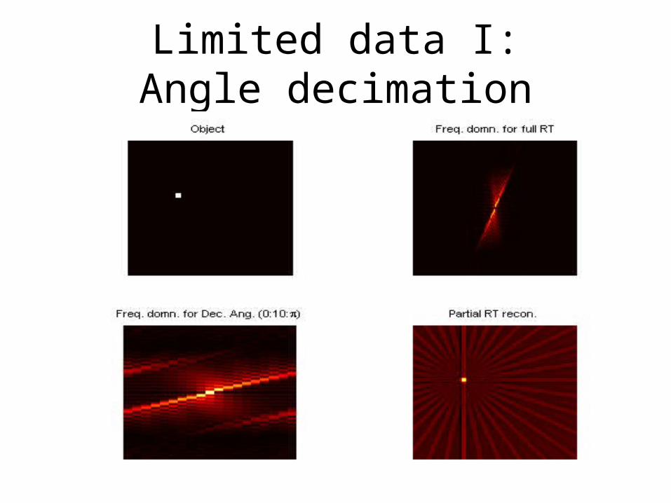
Limited data I:Angle decimation
These slides based almost entirely on a set provided by Prof. Eric Miller
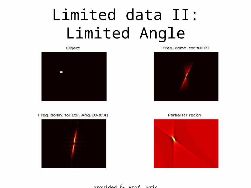
Limited data II:Limited Angle
These slides based almost entirely on a set provided by Prof. Eric Miller
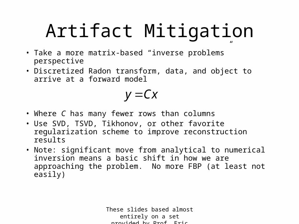
Artifact Mitigation• Take a more matrix-based “inverse problems” perspective• Discretized Radon transform, data, and object to arrive at a
forward model
• Where C has many fewer rows than columns• Use SVD, TSVD, Tikhonov, or other favorite
regularization scheme to improve reconstruction results• Note: significant move from analytical to numerical
inversion means a basic shift in how we are approaching the problem. No more FBP (at least not easily)
y Cx
These slides based almost entirely on a set provided by Prof. Eric Miller
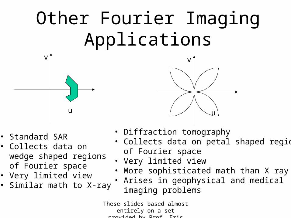
Other Fourier Imaging Applications
u
v
u
v
• Standard SAR• Collects data on wedge shaped regions of Fourier space• Very limited view• Similar math to X-ray
• Diffraction tomography• Collects data on petal shaped regions of Fourier space• Very limited view• More sophisticated math than X ray• Arises in geophysical and medical imaging problems
These slides based almost entirely on a set provided by Prof. Eric Miller
Generalized Radon Transforms
• Radon transform = integral of object over straight lines
• Many extensions– Integration over planes in 3D– Over circles in 2D (different type of SAR)– Over much more arbitrary mathematical structures
(asymptotic case of some acoustics problems with space varying background).
– Of weighted object function (attenuated Radon transform)


