
Tim Kallman (NASA/GSFC)
+ A. Dorodnitsyn (GSFC)
+ D. Proga (UNLV)
Warm absorbers from torus evaporative flows(??)
..

Why should we care about warm absorbers…
• Mass loss rate in wind < 0.1 Msun/yr • Mass accretion rate ~0.01 L44 Msun/yr • à warm absorber flows are important in the AGN
mass budget • Suggests that accretion inside warm absorber
launching may be easily disrupted: what determines how much gas makes it inward, past the torus?
• Torus origin consistent with warm absorber speeds, dust sublimation.
Questions..
● Can the (relatively) simple scenario, torus evaporation, explain warm absorber observed properties?
● To what extent does warm absorber modeling force us to understand (everything else about) the gas flows in AGN central regions?
● What are the key observed quantities (i.e. how can we tailor future efforts to maximize progress)

The challenge of understanding torus origin of warm absorbers
Wwarm absorber properties
torus properties
Accretion mechanism

Observational situation No. 2, 2010 AMD OF IRAS 13349+2438 985
Table 3Narrow Emission Lines
Line λRest λObserveda Flux
(Å) (Å) (10−5 photons s−1 cm−2)
Fe+0–Fe+9 Kα 1.94 1.940 ± 0.006b 1.0 ± 0.2Fe+10–Fe+16 Kα 1.93–1.94c 1.905 ± 0.006b 0.5 ± 0.1Fe+17–Fe+23 Kα 1.86–1.90d 1.877 ± 0.006b 0.4 ± 0.1Ne+8 forbidden 13.698 13.710 ± 0.012e 0.5 ± 0.1O+6 intercombination 21.801 21.794 ± 0.009e 3.5 ± 0.6O+6 forbidden 22.097 22.093 ± 0.009e 6 ± 1
Notes.a In the AGN rest frame.b FWHM = 15 mÅ.c Decaux et al. (1995).d Decaux et al. (1997).e FWHM = 235 km s−1.
3.4. Narrow Emission Lines
The present MCG –6-30-15 spectrum has a few narrow,bright emission lines of Fe, Ne, and O, which are assumednot to be absorbed by the outflow, but are absorbed by thelocal component discussed in Section 4.4 (and by the neutralGalactic column). These lines are fitted with simple Gaussiansand are found to be stationary to within ≈70 km s−1. The FeKα blends appear slightly broader (FWHM = 15 mÅ) than theNe and O lines whose widths are consistent with a kinematicbroadening of 235 km s−1 FWHM, as expected for featurescomprised of many lines from several charge states. The centroidwavelength and photon flux are measured for each feature andlisted in Table 3. The Kα emission by neutral Fe, or generallyM-shell Fe ions, is detected at 1.94 Å (6.4 keV). Weaker Kαemission from more highly ionized L-shell Fe is detected atsomewhat shorter wavelengths. Both of these are likely due toa moderately ionized medium excited by the continuum. TheNe+8 Kα forbidden line at 13.7 Å is less prominent, but canstill be detected. The O+6 Kα forbidden and intercombinationlines at 22.1 Å, and at 21.8 Å, respectively, are clearly detected.Conversely, the He-like resonance Kα lines of Ne and O arenot observed in emission. We believe these emission lines doexist since they are implied by the other He-like lines. However,because they overlap with the absorption lines from the slowoutflow (Section 4.2) they cannot be detected. This in turnmeans that we underestimate the absorption lines in thesetroughs. Kinematically therefore, the narrow emission linesmight originate in the slow outflow. Narrow X-ray emissionlines have been associated with the absorbing outflows inSeyfert galaxies based on the similar velocities, charge states,and column densities deduced for the emitting and absorbingplasma (Kinkhabwala et al. 2002; Behar et al. 2003). Note thatno emission lines from the fast component of −1900 km s−1
(Section 4.3) are detected. In fact, strongly blueshifted narrowemission lines are never detected, neither in the X-ray nor theUV, while slow winds of a few 100 km s−1 do produce narrowemission lines. Broad (2000 km s−1) emission lines that might beexpected if the fast component is quasi-spherically symmetricare also not observed and in any case not expected for lowcharge states, as the fast component is very highly ionized, asdiscussed below. All this seems to hint at the different physicalnature (e.g., opening angle and mass) of fast and slow outflows.
The non-shifted positions (∆v < 70 km s−1) and widths(FWHM < 250 km s−1) of the X-ray narrow emission linesare also consistent with that of the bright, forbidden O+2 optical
Figure 2. AMD of the slow outflow in MCG –6-30-15 obtained exclusively fromFe absorption and scaled by the solar Fe/H abundance 3.16 × 10⁻⁵ (Asplundet al. 2009). The corresponding temperature scale, obtained from the XSTARcomputation is shown at the top of the figure. The middle bin value is zero, andonly the upper limit uncertainty is plotted. The cumulative column density up toξ is plotted in the lower panel, yielding a total of NH = (5.3±0.7)×1021 cm−2.Dotted: blue lines represent the two ionization components of McKernan et al.(2007) broadened by their 3σ uncertainty of ∆ξ = 0.3 erg s−1 cm. Thecumulative column density of McKernan et al. (2007) is plotted as a blueline in the lower panel, yielding a total of NH = (7.0 ± 1.4) × 1021 cm−2.(A color version of this figure is available in the online journal.)
narrow emission lines at 4959 Å and 5007 Å, suggesting thatperhaps the X-ray line emitting region is in the optical narrowline region (NLR). The higher ionization optical (coronal) linesof ionized Fe appear to be much broader (FWHM ≈ 2000 kms−1; Reynolds et al. 1997), placing them closer to the nucleus.However, one has to wonder how robust these widths really are,given how faint these lines are in MCG –6-30-15 (see Figure 2in Reynolds et al. 1997).
4. RESULTS
4.1. Ionic Column Densities
The best-fit ionic column densities are listed in Table 4 andthe resulting model is plotted over the data in Figure 1. Theerrors for the ionic column densities were calculated in thesame manner as in Holczer et al. (2007). For the most part,the column densities in the slow component (−100 km s−1)of the Fe, Si, N, Ne, and Mg ions are of the order of 1016–1017 cm−2, while those of the more abundant O ions are higherand reach ∼1018 cm−2. Comparing our results with those ofSako et al. (2003), we find that Fe L-shell, Si K-shell, Mg

This behavior seems to be common to many
objects: • Ionization parameter:
apparently bimodal • V<2000 km/s • Column ~anticorrelated
with ionization
McKernan et al. 2007
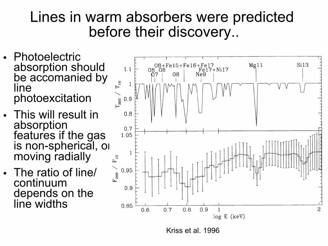
Lines in warm absorbers were predicted before their discovery..
• Photoelectric absorption should be accomanied by line photoexcitation
• This will result in absorption features if the gas is non-spherical, or moving radially
• The ratio of line/continuum depends on the line widths
Kriss et al. 1996

The torus ● To make obscuration:
R ⇠ 1 pc⌧Th
= 10nTorus
' 105 cm�3 ⌧Th
R�1pc
MTorus
' 106M�⌧Th
R2pc
Tvir
= 5⇥ 105 K M6R�1pc
• Vertical Support:
HR =
qT
TV ir
HR =
qaT 4
nkTV ir
1986ApJ...308L..55K
(Krolik and Begelman 1986)
(Jaffe et al. 2004)
out 4 for a variety of reasons, and confirmed only 3 asunabsorbed Sy 2s. Using a variety of metrics for a criticalassessment of 24 objects that were previously claimed to beunabsorbed Sy 2s (again including many from Panessa &Bassani 2002), Shi et al. (2010) could confirm only two asgenuine, with broad emission lines 2–3 orders of magnitudefainter than typical Sy 1s—although several more candidatesmay have anomalously weak broad lines, this could not beconfirmed with existing data. These authors concluded that 1%or less of Sy 2s are X-ray unabsorbed.
In contrast, a much higher fraction of such sources—30% ofAGNs at ∼−Llog 4314 195 —appears in the Merloni et al. (2014)sample. Whether this indicates that there is a large population
of X-ray unabsorbed Sy 2s or is due to a classification bias wasdiscussed in depth by these authors. With reference to stackedoptical spectra and spectral energy distributions, they suggestedthat many of the lower luminosity AGNs may have beenincorrectly photometrically classified as Sy 2 due to the lowcontrast of the AGNs against the relatively bright host galaxy.On the other hand, spectroscopic data are sensitive to featuresassociated with Sy 1s, such as broad lines, even when they areweak. Such signatures would not be evident in broad-bandintegrated photometry. This difference is reflected in their data:while 77% of the AGNs with only integrated broad-bandphotometric data are classified as Sy 2, only 56% of AGNs withspectroscopic data are classified as Sy 2s. The lower totalfraction of Sy 2s based on spectroscopic classifications impliesin turn a much lower fraction of X-ray unabsorbed Sy 2s.Figure 6 shows that in our volume limited sample of Swift-
BAT AGNs, there are no sources classified as X-ray unabsorbedSy 2, implying these sources are rare. In this context, asimulation of the AGN population can provide valuable insight,since we know the Sy 2 fractions in both flux limited andvolume limited samples. We describe this simulation inSection 4.3, aiming to answer the question of which curvefrom Merloni et al. (2014) in Figure 7 properly traces thefraction of Sy 2s: is it types 22 + 21 or just type 22?
4.3. A Simulated Swift-BAT sample
Our aim here is to simulate parent populations of AGNs withdifferent prescriptions for the intrinsic fraction of Sy 2s. Afterapplying observational limits, we can then use constraints fromthe flux-limited sample of Winter et al. (2009) and our ownvolume-limited sample to discriminate between the differentprescriptions, giving us a handle on the true fraction of Sy 2s.We begin by constructing a population of AGNs using a
2–10 keV luminosity function from Aird et al. (2010) suitablefor low redshift:
ϕ ∝ +− − −−⎡
⎣⎢⎤⎦⎥( ) ( ) ( )L L L L L2 10
int2 10int
00.70
2 10int
03.14 1
where =Llog 44.960 . We have then randomly assigned eachAGN to be a Sy 1 or Sy 2 according to the obscured fraction asa function of luminosity. We use two functions, which arediscussed below. We allow the AGNs to be observed bycalculating −L14 195 from −L2 10
int , assigning them random locationsin a local volume, deriving their fluxes, and assessing whetherthey would be detected in the Swift-BAT survey. In doing this,we have not included the effects of X-ray absorption in the14–195 keV band since, as we have seen, it has little impact atsuch high energies for the absorbing columns expected. We usea limit appropriate for the 9 months survey in order to select aflux limited sample matching that used by Winter et al. (2009);and a limit appropriate for the 58 months survey to match ourvolume limited selection outlined in this paper.The left panels in Figure 8 show the two obscuration
functions used in our simulations. The dotted line in the upperleft panel is taken directly from Merloni et al. (2014) and wasdesigned to follow the curve for types 22+21; the dashed line inthe lower left panel is our modification of this function tomatch the type 22 data, those AGNs that are both opticallyobscured and X-ray absorbed. The results of our simulationsusing these functions are also given in Figure 8. The center
Figure 6. Fractions of optically obscured and X-ray absorbed AGNs in ourcomplete volume limited Swift-BAT sample (see also Figure 7). The first/second digit of the type codes for optical/X-ray obscuration as described inSection 4.1. The black lines denote the strict definitions. The gray lines showthe impact of relaxing the definitions slightly: the three type 12 AGNs would bereclassified as one type 11 and two type 22.
Figure 7. Fractions of optically and X-ray obscured AGNs as a function ofluminosity. The curves are adapted from Figure 12 of Merloni et al. (2014).The details of the types, defined by those authors, are summarized inSection 4.3: the first/second digit of the type codes for optical/X-rayobscuration. The luminosity scale has been derived from −L2 10
int as indicatedin Section 3. The black ranges refer to our sample, and indicate the impact ofallowing some flexibility in the definition of optically obscured and X-rayabsorbed. At overlapping luminosities, the sample have similar fractions ofAGNs that are X-ray absorbed (types 22+12) and that are both X-ray absorbedand optically obscured (type 22); but the fractions of AGNs classified as Sy 2(types 22+21) are very different.
9
The Astrophysical Journal, 806:127 (14pp), 2015 June 10 Davies et al.
(Davies et al. 2015)

Torus Evaporation:
1981ApJ...249..422K
In a heated hydrostatic atmosphere, gas is expected to remain in warm/cold phase when pressure exceed Pmin At lower pressure gas heats toward Compton temperature, ~ 107K
Pmin ' L4⇡R2⌅⇤
cc
m ⇠ Pmin
cs' 10�13 gm s�1 cm�2 L44R�2
pc T�17 ⌅
M ' 0.1M� yr�1 L44T�17 ⌅
tevap = MTorus
M' 107 yrs
tdyn =q
R3
2GMBH' 104 yrs R3/2
pc M�1/26
tHeat ' 2⇥ 104 yrs TTIC
R2pcL
�144
à X-ray heating will produce a thermally driven outflow in approximate equilibrium with the illuminating radiation
(Krolik McKee Tarter 1982)
Wind/warm absorber
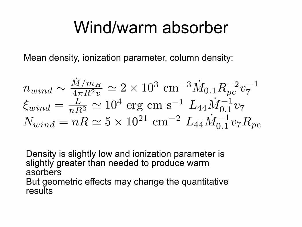
nwind ⇠ M/mH
4⇡R2v ' 2⇥ 103 cm�3M0.1R�2pc v
�17
⇠wind = LnR2 ' 104 erg cm s�1 L44M
�10.1 v7
Nwind = nR ' 5⇥ 1021 cm�2 L44M�10.1 v7Rpc
Mean density, ionization parameter, column density:
Density is slightly low and ionization parameter is slightly greater than needed to produce warm asorbers But geometric effects may change the quantitative results

§ Assume a torus at ~1 pc about a 106Msun black hole
§ Initial structure is constant angular momentum adiabatic (cf. Papaloizou and Pringle 1984)
§ This structure is stable (numerically) for >20 rotation periods
§ Choose T~Tvir, n~108 cm-3 for unperturbed torus
§ Calculate hydrodynamics in 2.5d (2d + axisymmetry) (Zeus2d)
§ Add illumination by point source of X-rays at the center
§ Include physics of X-ray heating, radiative cooling --> evaporative flow (cf. Blondin 1994)
§ Also radiative driving due to UV lines (cf. Castor et al. 1976; Stevens & K. 1986)
§ Formulation similar to Proga et al. 2000, Proga & K. 2002, 2004
Dynamical calculations
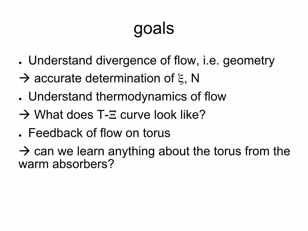
goals
● Understand divergence of flow, i.e. geometry à accurate determination of ξ, N ● Understand thermodynamics of flow à What does T-Ξ curve look like? ● Feedback of flow on torus à can we learn anything about the torus from the warm absorbers?
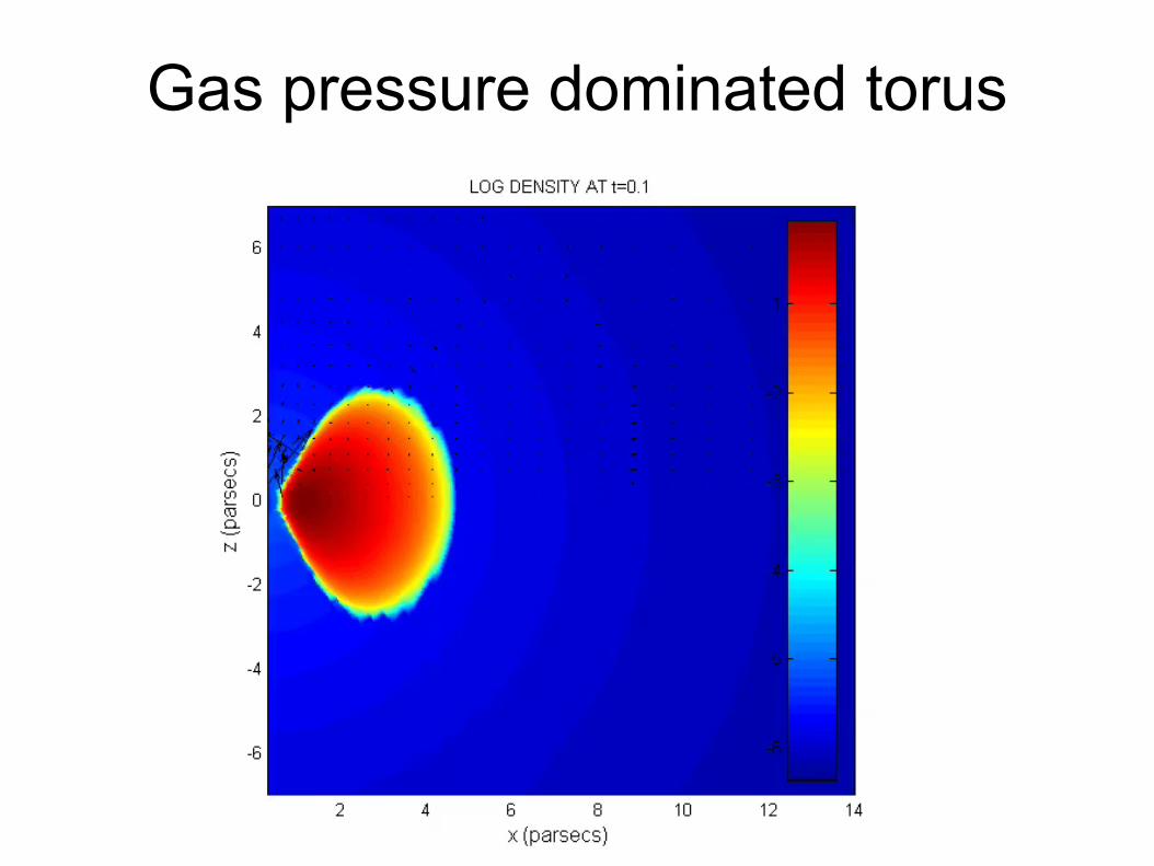
Gas pressure dominated torus

Column density vs. inclination
• Column is ~1024 cm-3
for inclinitions >45 initially
• Torus thins with time • Very rapid transition
from thick to thin at most times

2 2.5 3 3.5 4
00.
51
inclination= 1.5
log(energy (eV))
log(
trans
mitt
ed fl
ux)
−2 0 2 4−6−4
−20
2
inclination= 1.5
log(xi)
log(
AMD
(Tho
mso
n))
2 2.5 3 3.5 4
00.
51
1.5
inclination= 1.4
log(energy (eV))
log(
trans
mitt
ed fl
ux)
−2 0 2 4−6−4
−20
2
inclination= 1.4
log(xi)
log(
AMD
(Tho
mso
n))
2 2.5 3 3.5 4
0.5
11.
52
inclination= 1.2
log(energy (eV))
log(
trans
mitt
ed fl
ux)
−2 0 2 4−6−4
−20
2
inclination= 1.2
log(xi)
log(
AMD
(Tho
mso
n))
2 2.5 3 3.5 4
11.
52
2.5
inclination= 1.0
log(energy (eV))
log(
trans
mitt
ed fl
ux)
−2 0 2 4−6−4
−20
2
inclination= 1.0
log(xi)
log(
AMD
(Tho
mso
n))
2 2.5 3 3.5 4
11.
52
2.5
inclination= 0.8
log(energy (eV))
log(
trans
mitt
ed fl
ux)
−2 0 2 4−6−4
−20
2
inclination= 0.8
log(xi)
log(
AMD
(Tho
mso
n))
2 2.5 3 3.5 4
0.5
11.
52
2.5
inclination= 0.7
log(energy (eV))
log(
trans
mitt
ed fl
ux)
−2 0 2 4−6−4
−20
2
inclination= 0.7
log(xi)
log(
AMD
(Tho
mso
n))
2 2.5 3 3.5 4
0.5
11.
52
2.5
inclination= 0.5
log(energy (eV))lo
g(tra
nsm
itted
flux
)−2 0 2 4−6
−4−2
02
inclination= 0.5
log(xi)
log(
AMD
(Tho
mso
n))
2 2.5 3 3.5 4
0.5
11.
52
2.5
inclination= 0.3
log(energy (eV))
log(
trans
mitt
ed fl
ux)
−2 0 2 4−6−4
−20
2
inclination= 0.3
log(xi)
log(
AMD
(Tho
mso
n))
Warm absorber spectra
● Spectra shown at intermediate time ● At i~90o see AMD~few x Thomson across many
ionization parameters ● Obscuration angle ~+-30o
● at lower angles see weak, highly ionized warm absorber
● Plausible warm absorber only in narrow range of angles near ~30o
● weak evidence for thermal instability/2 phase behavior

Fit to Chandra HETG spectrum of NGC 3783
10 12 14 16 18 20
05×
10−1
910
−18
1.5×
10−1
82×
10−1
82.
5×10
−18
norm
aliz
ed c
ount
s s−
1 Hz−
1
Wavelength (Å)
model 2 fit
tim 11−Dec−2008 17:12
Misses UTA due to absence of low ionization gas

What happens to gas in the T-ξ/T plane in such a model..
Log(ξ/T)
Lessons from gas-pressure dominated torus models
● Outflow mass loss rate is comparable to estimates, it shapes the torus
● Line profiles, ionization, blueshift ~consistent with observations.
● Density in torus throat is similar to spherically diverging flow à warm absorbers are seen for relatively narrow range of viewing angles
● Adiabatic cooling is important à no obvious 2 phase behavior
● Outflow depends on torus structure; unphysical gas pressure dominated torus does not fit with standard unification.
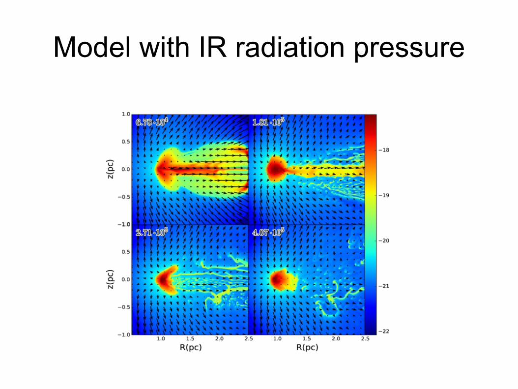
Model with IR radiation pressure
● IR generated by reprocessing of X-rays according to simple prescription
● IR transfer uses flux limited diffusion ● Include all X-ray thermal and pressure effects from gas-
pressure models ● Models are 2.5D axisymmetric (zeusmp) ● Hydrodynamic viscosity is also included to maintain
balance with radiation pressure ● X-ray excited wind contributes to accretion ● Cf. Krolik 2007, Shi and Krolik 2008, Chan and Krolik
2016…

Model with IR radiation pressure
Model with IR radiation pressure
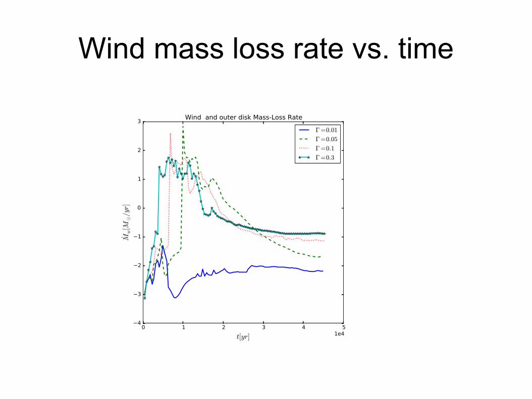
Wind mass loss rate vs. time
the time evolution of our simulations is shown. The totalnumber of models shown N 100mod = .
When 0.01G = , the episode of disk accretion leads to asignificant depletion of the gas, and thus this set of models hasa lower proportion of obscuring models at any inclination. As Γincreases, no more episodes of disk accretion are observed anda larger radiation input leads to larger aspect ratios. Thedistributions of the column densities are broader at higherradiation input, reflecting the importance of radiation pressure.The results are that a model with 0.01G = has the smallest anda model with 0.3G = has the largest aspect ratio of the torus.
The region of the torus which is truly Thomson thick subtendsa polar angle 40~ at most (for 0.3G = ); lower columndensities extend to 80~ .
6. DISCUSSION
In our previous work we adopted a pre-existing thinaccretion disk as a boundary condition. This allowed us tostudy quasi-stationary accretion disk wind solutions but did notallow us to address the question of whether accretion can bestopped by radiation pressure and heating effects. Togetherwith these earlier findings, our current results suggest that,qualitatively, obscuration can proceed in accretion or outflowmode, depending on the radiative input. The first scenariocomprises a global accretion flow that is slowed, puffed up, andkept geometrically thick by IR radiation pressure. The seconddescribes a radiation-driven obscuring outflow. There is also anintermediate mode in which the equatorial accretion disk issurrounded by a slowly in- or outflowing envelope. Thequantitative boundaries between these scenarios depend ondetails of heating/cooling, dust formation, and destruction.Some of results presented here may be sensitive to the
assumptions regarding microphysics or computational simpli-fications. A simple analytical model developed in Paper I ofthis series predicts that as the temperature of the dusty gasreaches T n M r987vir, r 7
1 471 4
pc1 4-� K the radiation pressure in
the optically thick regime becomes larger than gravity andoutflow begins. This is confirmed in the current studies. Forexample, the dynamics of the torus depends primarily on theenergy density of infrared radiation and on the ratio of the dustopacity to the opacity of the fully ionized gas, edk k , makingthe radiation pressure launching of the wind depend on howdust is treated. In this paper we adopt relatively simpleassumptions about the dust formation and destruction. In laterwork we plan to examine in more detail the effects of thetreatment of dust formation on the hydrodynamics.
Figure 8. Time dependence of the total wind mass-loss rate, Mw˙ , for fiducial L LeddG = (left) and the energy of the vertical wind (right).
Figure 9. The logarithm of the number of models which at the giveninclination have an optical depth larger than one. X-axis: the inclination anglein degrees measured from the axis of rotation. Colors indicate different L Ledd.
13
The Astrophysical Journal, 819:115 (15pp), 2016 March 10 Dorodnitsyn, Kallman, & Proga
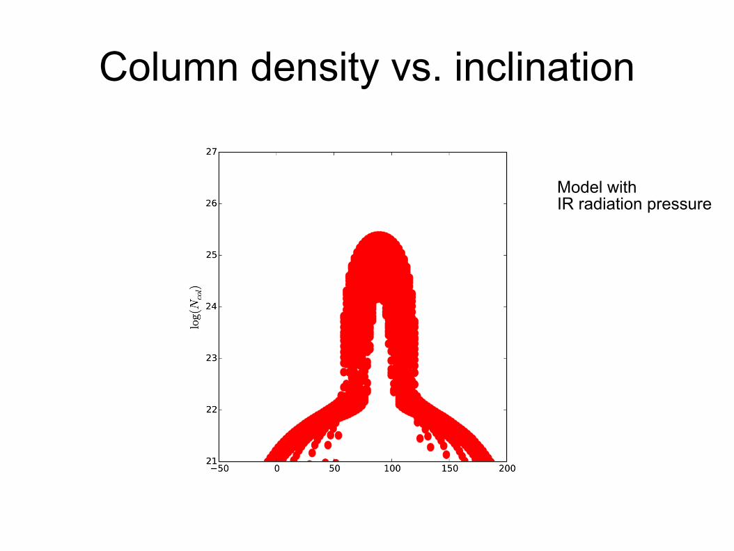
Column density vs. inclination
Model with IR radiation pressure

2 2.5 3 3.5 4
00.
51
inclination= 1.5
energy
inte
nsity
−2 0 2 4−6−4
−20
2
inclination= 1.5
log(xi)
log(
AMD
(Tho
mso
n))
2 2.5 3 3.5 4
00.
51
inclination= 1.4
energy
inte
nsity
−2 0 2 4−6−4
−20
2
inclination= 1.4
log(xi)
log(
AMD
(Tho
mso
n))
2 2.5 3 3.5 4
0.5
11.
52
inclination= 1.2
energy
inte
nsity
−2 0 2 4−6−4
−20
2
inclination= 1.2
log(xi)
log(
AMD
(Tho
mso
n))
2 2.5 3 3.5 4
11.
52
2.5
inclination= 1.0
energy
inte
nsity
−2 0 2 4−6−4
−20
2
inclination= 1.0
log(xi)
log(
AMD
(Tho
mso
n))
2 2.5 3 3.5 4
1.5
22.
5
inclination= 0.8
energy
inte
nsity
−2 0 2 4−6−4
−20
2
inclination= 0.8
log(xi)
log(
AMD
(Tho
mso
n))
2 2.5 3 3.5 4
1.5
22.
5
inclination= 0.7
energy
inte
nsity
−2 0 2 4−6−4
−20
2
inclination= 0.7
log(xi)
log(
AMD
(Tho
mso
n))
2 2.5 3 3.5 4
22.
5
inclination= 0.5
energyin
tens
ity−2 0 2 4−6
−4−2
02
inclination= 0.5
log(xi)
log(
AMD
(Tho
mso
n))
2 2.5 3 3.5 4
1.8
22.
22.
4inclination= 0.3
energy
inte
nsity
−2 0 2 4−6−4
−20
2
inclination= 0.3
log(xi)
log(
AMD
(Tho
mso
n))
Warm absorber spectra
● Spectra shown at intermediate time ● At i=π/2 see AMD~few across many ionization
parameters ● Results for obscuration angle and range of
warm absorber observations are similar to gas pressure dominated case
● Mass requirement is lower due to pressure support
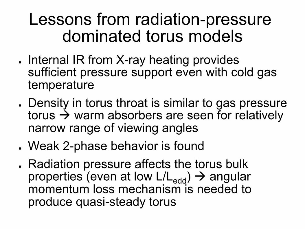
Lessons from radiation-pressure dominated torus models
● Internal IR from X-ray heating provides sufficient pressure support even with cold gas temperature
● Density in torus throat is similar to gas pressure torus à warm absorbers are seen for relatively narrow range of viewing angles
● Weak 2-phase behavior is found ● Radiation pressure affects the torus bulk
properties (even at low L/Ledd) à angular momentum loss mechanism is needed to produce quasi-steady torus

Mhd torus
• 3d MHD models (Athena) • X-ray heating included • No IR radiation pressure • Two different initial magnetic field
configurations considered • configuration based on tokamak solution à strong initial poloidal field both inside and outside torus (SOL)
• Configuration with field proportional to gas density (TOR)
l
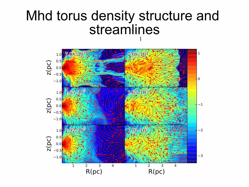
Mhd torus density structure and streamlines
l
– 34 –
Fig. 5.— Color plot of the density, log ⇢ for Lx = 0.25Ledd, (� = 0.5, fx = 0.5), superimposed
with the velocity stream lines. Shown are di↵erent times given in years. Left column: SOL
models; right column: TOR models. Axes: horizontal: z: distance from equatorial plane in
parsecs; R: distance from the BH in parsecs.
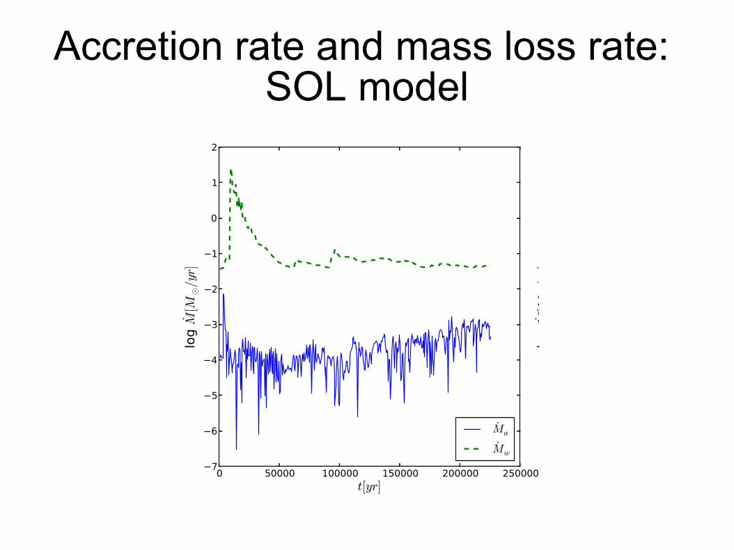
Accretion rate and mass loss rate: SOL model
– 39 –
Fig. 10.— Accretion rate, Ma and the total wind mass-loss rate, Mw versus time for two
di↵erent initial setups: Left: SOL; right: TOR
Fig. 11.— Scatter plot showing the logarithm of the column density, Ncol(cm�2). Each
recorded simulation time is represented by a point. Left: SOL; right: TOR

Column density vs. inclination
MHD model
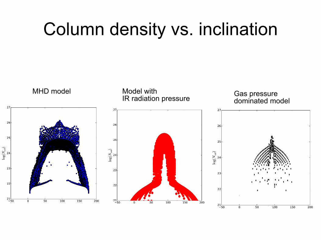
Column density vs. inclination
MHD model Model with IR radiation pressure
Gas pressure dominated model
2 2.5 3 3.5 4
00.
10.
2inclination= 1.5
energy
inte
nsity
−2 0 2 4−6−4
−20
2
inclination= 1.5
log(xi)
log(
AMD
(Tho
mso
n))
2 2.5 3 3.5 4
00.
10.
20.
3
inclination= 1.4
energy
inte
nsity
−2 0 2 4−6−4
−20
2
inclination= 1.4
log(xi)
log(
AMD
(Tho
mso
n))
2 2.5 3 3.5 4
00.
10.
20.
30.
4
inclination= 1.2
energy
inte
nsity
−2 0 2 4−6−4
−20
2
inclination= 1.2
log(xi)
log(
AMD
(Tho
mso
n))
2 2.5 3 3.5 4
00.
20.
40.
60.
8
inclination= 1.0
energy
inte
nsity
−2 0 2 4−6−4
−20
2
inclination= 1.0
log(xi)
log(
AMD
(Tho
mso
n))
2 2.5 3 3.5 4
00.
51
inclination= 0.8
energy
inte
nsity
−2 0 2 4−6−4
−20
2
inclination= 0.8
log(xi)
log(
AMD
(Tho
mso
n))
2 2.5 3 3.5 4
00.
51
1.5
inclination= 0.7
energy
inte
nsity
−2 0 2 4−6−4
−20
2
inclination= 0.7
log(xi)
log(
AMD
(Tho
mso
n))
2 2.5 3 3.5 40
0.5
11.
5
inclination= 0.5
energy
inte
nsity
−2 0 2 4−6−4
−20
2
inclination= 0.5
log(xi)
log(
AMD
(Tho
mso
n))
2 2.5 3 3.5 4
00.
51
1.5
inclination= 0.3
energy
inte
nsity
−2 0 2 4−6−4
−20
2
inclination= 0.3
log(xi)
log(
AMD
(Tho
mso
n))
2 2.5 3 3.5 4
00.
10.
2inclination= 1.5
energy
inte
nsity
−2 0 2 4−6−4
−20
2
inclination= 1.5
log(xi)
log(
AMD
(Tho
mso
n))
2 2.5 3 3.5 4
00.
10.
20.
3
inclination= 1.4
energy
inte
nsity
−2 0 2 4−6−4
−20
2
inclination= 1.4
log(xi)
log(
AMD
(Tho
mso
n))
2 2.5 3 3.5 4
00.
10.
20.
30.
4
inclination= 1.2
energy
inte
nsity
−2 0 2 4−6−4
−20
2
inclination= 1.2
log(xi)
log(
AMD
(Tho
mso
n))
2 2.5 3 3.5 4
00.
20.
40.
60.
8
inclination= 1.0
energy
inte
nsity
−2 0 2 4−6−4
−20
2
inclination= 1.0
log(xi)
log(
AMD
(Tho
mso
n))
2 2.5 3 3.5 4
00.
51
inclination= 0.8
energy
inte
nsity
−2 0 2 4−6−4
−20
2
inclination= 0.8
log(xi)
log(
AMD
(Tho
mso
n))
2 2.5 3 3.5 4
00.
51
1.5
inclination= 0.7
energy
inte
nsity
−2 0 2 4−6−4
−20
2
inclination= 0.7
log(xi)
log(
AMD
(Tho
mso
n))
2 2.5 3 3.5 40
0.5
11.
5
inclination= 0.5
energy
inte
nsity
−2 0 2 4−6−4
−20
2
inclination= 0.5
log(xi)
log(
AMD
(Tho
mso
n))
2 2.5 3 3.5 4
00.
51
1.5
inclination= 0.3
energy
inte
nsity
−2 0 2 4−6−4
−20
2
inclination= 0.3
log(xi)
log(
AMD
(Tho
mso
n))

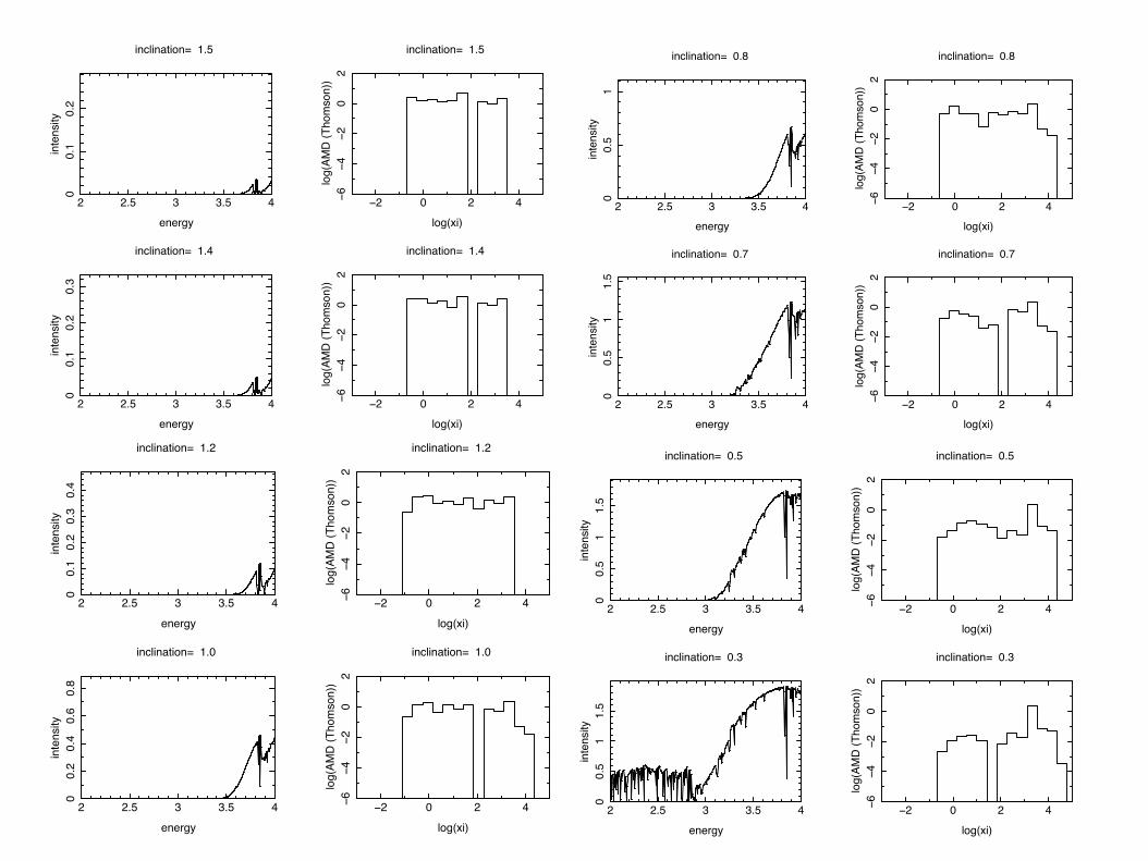
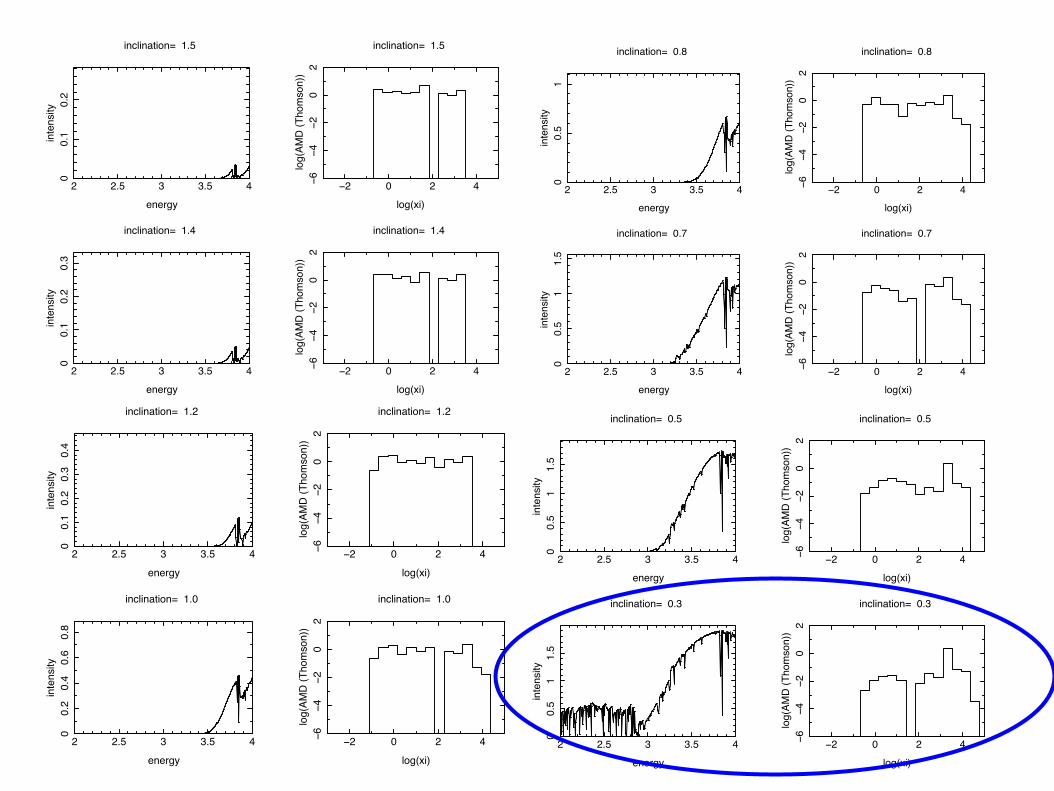
Warm absorber spectra
● Spectra shown at intermediate time ● Model provides obscuration over many lines of
sight ● Much more obscuration compared with
previous models ● Warm absorber produced only for lines of sight
close to axis
Lessons from MHD torus models
● With strong poloidal initial field, evaporation rate is suppressed by large factor
● 2-phase behavior is apparent – Due to impeded flow/dilution? – Or?
● Long-lived torus provides obscuration over large range of viewing angles for longer time
● Torus structure/evolution depends strongly on field topology
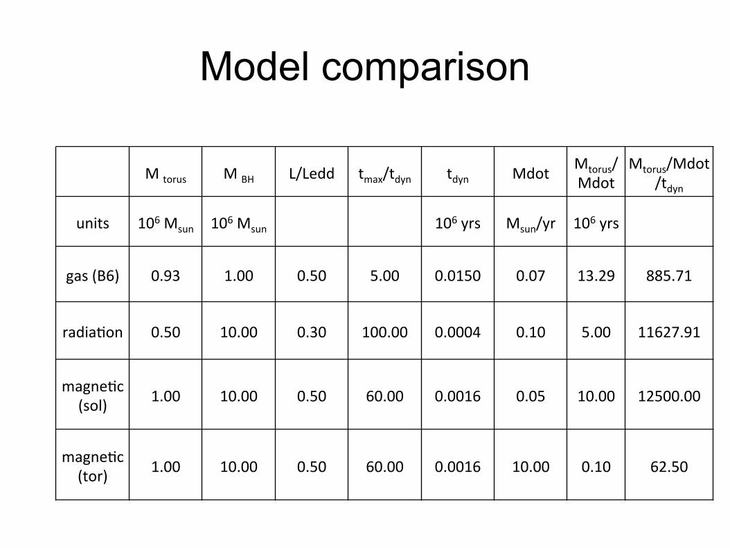
Model comparison
Mtorus MBH L/Ledd tmax/tdyn tdyn Mdot Mtorus/Mdot
Mtorus/Mdot/tdyn
units 106Msun 106Msun 106yrs Msun/yr 106yrs
gas(B6) 0.93 1.00 0.50 5.00 0.0150 0.07 13.29 885.71
radiaAon 0.50 10.00 0.30 100.00 0.0004 0.10 5.00 11627.91
magneAc(sol) 1.00 10.00 0.50 60.00 0.0016 0.05 10.00 12500.00
magneAc(tor) 1.00 10.00 0.50 60.00 0.0016 10.00 0.10 62.50
summary ● Models show evaporative wind from torus ‘throat’, mass loss rate
comparable to estimates à What is the torus?
● Ionization parameter and column are outside observed range for lines of sight close to axis
● Plausible warm absorbers are produced within a ~10o cone near the torus à what is the true incidence of warm absorbers?
● Trapped IR radiation pressure produces a torus with lower mass, comparable obscuration à long term survival?
● A strong (β~100) poloidal magnetic field can retard torus evaporation à self-gravity?


