Download - Ton van den Bogert - Cleveland State University

Ton van den Bogert

Department of Mechanical Engineering

Cleveland State University

SPACE-TIME METHODS FOR

TRAJECTORY OPTIMIZATION

Motivation: design

• Devices for sports and rehabilitation

• Goal: improve human movement

• Design usually based on “normal

movement” data

• Human response is not considered or predicted

• Prototyping and human testing needed

• Predictive simulation of human movement

can speed up the development process

• Results must be good enough

• Results must be obtained quickly

Simulation of movement

• Model is represented by differential equation

• Simulation is normally done forward in time, e.g.

• This is appropriate for many applications

• But not always…

u)f(x,x

x: state variables

u: control inputs

)()()()( tththt u,xfxx Euler method

[t,x] = ODE23(’f’, x0) Matlab

variable step solver

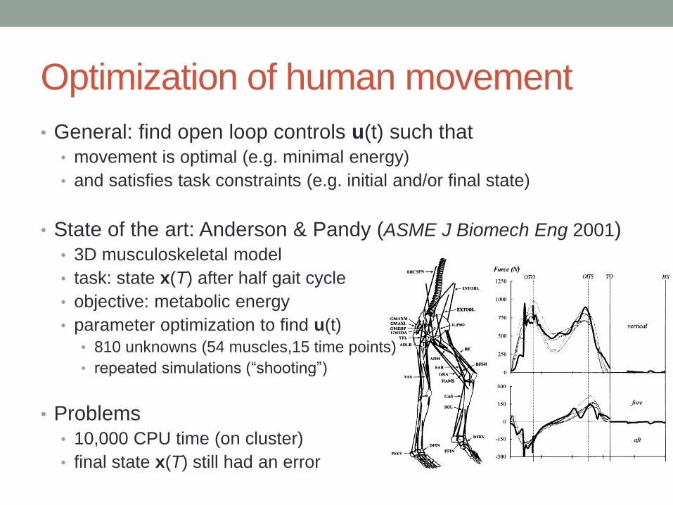
Optimization of human movement

• General: find open loop controls u(t) such that

• movement is optimal (e.g. minimal energy)

• and satisfies task constraints (e.g. initial and/or final state)

• State of the art: Anderson & Pandy (ASME J Biomech Eng 2001)

• 3D musculoskeletal model

• task: state x(T) after half gait cycle

• objective: metabolic energy

• parameter optimization to find u(t)

• 810 unknowns (54 muscles,15 time points)

• repeated simulations (“shooting”)

• Problems

• 10,000 CPU time (on cluster)

• final state x(T) still had an error

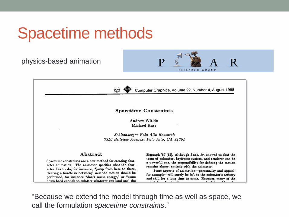
Spacetime methods

physics-based animation

“Because we extend the model through time as well as space, we

call the formulation spacetime constraints.”

The main idea

• Do not use simulation to find x(t)

• Iterate x(t) and u(t) until:

• movement is optimal

• satisfies task constraints

• satisfies physics constraints:

• Luxo lamp

• 2D, 6 DOF

• 3 torque actuators

• objective: minimal energy

• task: initial and final state

u)f(x,x

Book & aerospace applications

EXAMPLE: PENDULUM

SWING-UP

1-DOF pendulum

• Variables • angle x, torque u

• System dynamics:

• Task constraints for swing-up problem:

• Initial state

• Final state

• Cost function: integral of squared torque

x uxmgdxI sin

d

xd sin

mg

0)0(,0)0( xx 0)(,)( TxTx

T

dttu

0

2)(

Temporal discretization

• Direct collocation: N nodes

• Time step

• States controls

• Dynamics becomes algebraic constraints:

• Cost function becomes an algebraic function:

• Time step h usually much larger than in ODE solver • Convergence study to decide how many nodes are needed

• For human gait cycle: N=50 or N=100 is typically good enough

uxmgdxI sin iiiii uxmgd

h

xxxI

sin2

2

11

i

iu2

Nxxx 21, Nuuu 21,

t

x(t)

u(t)

t

h

1 2 3 … N

)1/( NTh

Constrained optimization problem

• Unknowns

• Minimize

• Subject to

• Matlab solvers for this type of problem:

• fmincon sequential quadratic programming

• SNOPT sequential quadratic programming (large scale)

• IPOPT interior point method (large scale)

TNN uuuxxx 2121 ,,,y

)(yf

0)( yc

cost function

task constraints and dynamics constraints

Matlab demo

using the Matlab code in pend.m

Planar musculoskeletal gait model

• 7 body segments, 9 DOF

• 16 Hill-based muscles

• Matlab MEX function

• download at Dynamic Walking 2011

• Find optimal gait

• objective function?

u)f(x,x

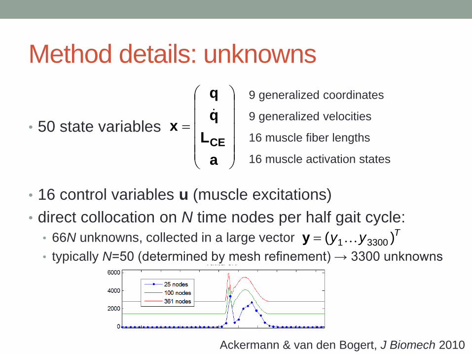
Method details: unknowns

• 50 state variables

• 16 control variables u (muscle excitations)

• direct collocation on N time nodes per half gait cycle:

• 66N unknowns, collected in a large vector

• typically N=50 (determined by mesh refinement) → 3300 unknowns

Ackermann & van den Bogert, J Biomech 2010

a

L

q

q

xCE

9 generalized coordinates

9 generalized velocities

16 muscle fiber lengths

16 muscle activation states

Tyy )( 33001y

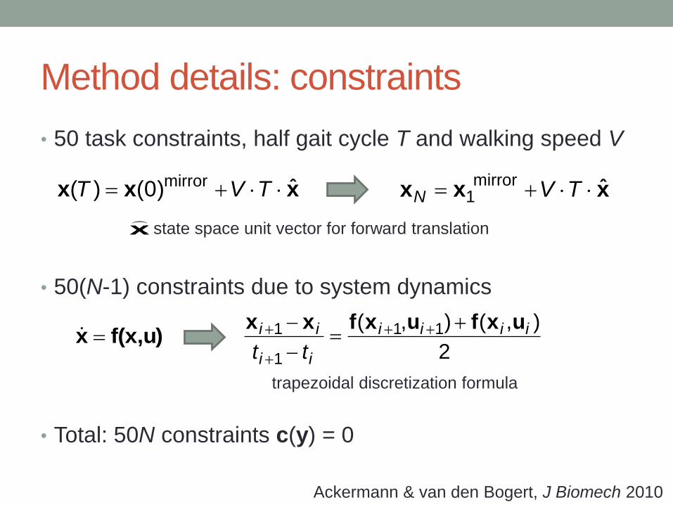
Method details: constraints

• 50 task constraints, half gait cycle T and walking speed V

• 50(N-1) constraints due to system dynamics

• Total: 50N constraints c(y) = 0


x

xxx ˆmirror1 TVNxxx ˆ)0()( mirror TVT

: state space unit vector for forward translation

u)f(x,x 2

),(),( 11

1

1 iiii

ii

ii

tt

uxfuxfxx

trapezoidal discretization formula

Method details: objective function

(cost function)

• For example, activation-based, M muscles:

• General form:


N

i

M

j

pj

jij

awwNM

f1 1

1

)(yf

wj: weighting of muscle j

exponent p = 2,3,…

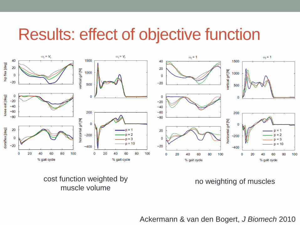
Results: effect of objective function


cost function weighted by

muscle volume no weighting of muscles

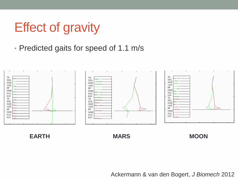
Effect of gravity

• Predicted gaits for speed of 1.1 m/s


EARTH MARS MOON

METHOD IMPROVEMENTS

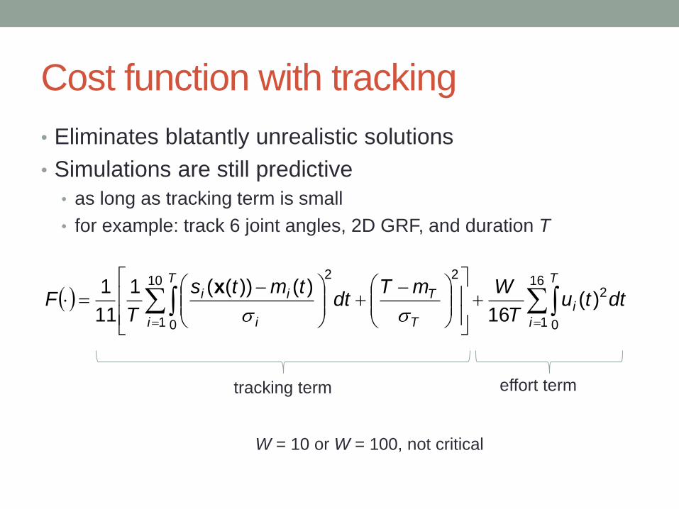
Cost function with tracking

• Eliminates blatantly unrealistic solutions

• Simulations are still predictive

• as long as tracking term is small

• for example: track 6 joint angles, 2D GRF, and duration T

16

1 0

210

1 0

22

)(16

)())((1

11

1

i

T

i

i

T

T

T

i

ii dttuT

WmTdt

tmts

TF

x

tracking term effort term

W = 10 or W = 100, not critical

Combined human/device model

• Hydraulic energy-storing knee

• Simultaneous optimal control of 10 muscles and 2 valves

prosthetic side (blue curves):

knee function is not restored

but it is the ankle’s fault!

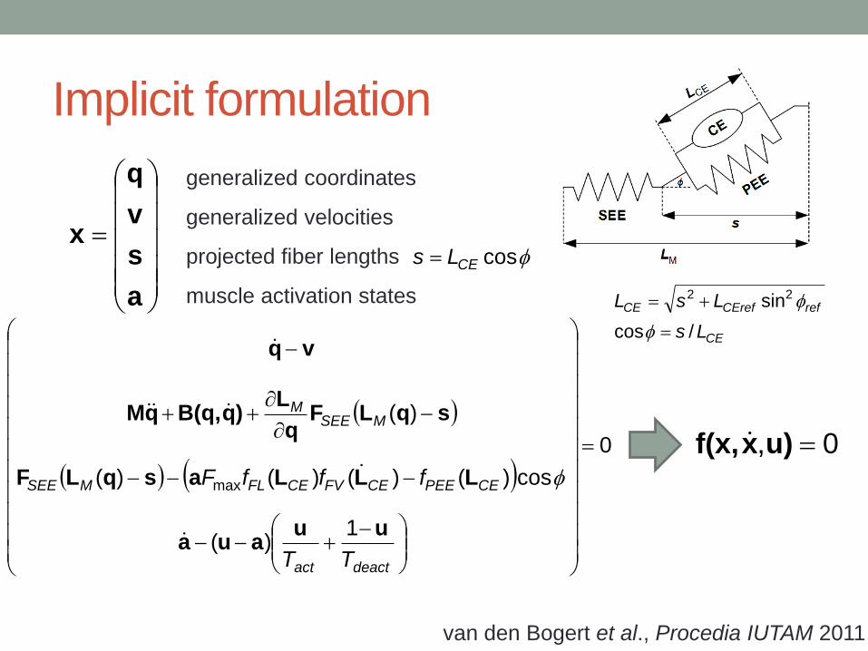
Implicit formulation

van den Bogert et al., Procedia IUTAM 2011

0, u)xf(x,

a

s

v

q

x

generalized coordinates

generalized velocities

projected fiber lengths

muscle activation states

cosCELs

0

1)(

cos)()()()(

)(

max

deactact

CEPEECEFVCEFLMSEE

MSEEM

TT

fffF

uuaua

LLLasqLF

sqLFq

L)qB(q,qM

vq

CE

refCErefCE

Ls

LsL

/cos

sin22

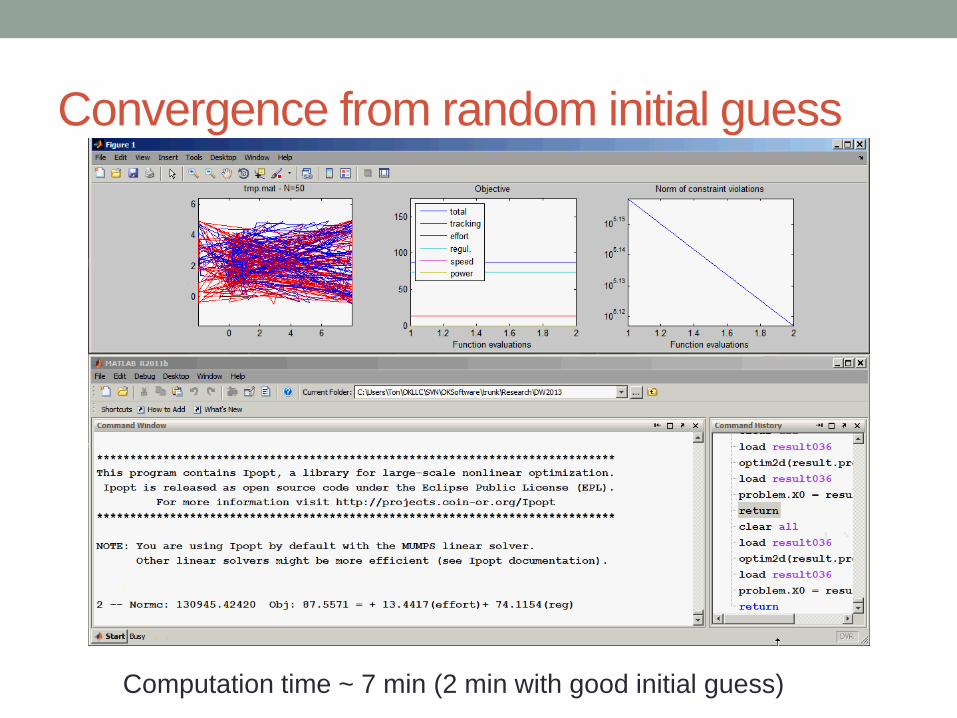
Convergence from random initial guess

Computation time ~ 7 min (2 min with good initial guess)

19 runs with random initial guess

• 3 runs did not converge

• 3 runs found the same solution (with cost 0.07)

• was also found from “intelligent” initial guesses

• 13 locally optimal solutions with higher cost

cost 0.071 cost 0.158

Discovering strategies for novel tasks

• Walk with a somersault in each step:

• Solution could only be found from random initial guess

31ˆ2ˆ0 xxxx TvT

mirror

Summary

• Trajectory optimization • in biomechanics known as “predictive simulation” because it can be

done without tracking human motion data

• direct collocation method was presented

• can include “hard” task constraints

• Many unknowns: discretized state and control trajectories • must use gradient-based solvers

• can fail to converge

• can even fail to produce a movement that is physically possible

• even if converged, solution can be a local optimum

• Trajectory optimization finds optimal open loop controls • this is not yet a controller!

Download - Ton van den Bogert - Cleveland State University

Top Related