Transfers, Bequests, and Human Capital Investment in Children over the Lifecycle
Eric French University College London and Institute for Fiscal Studies
Andrew Hood
Institute for Fiscal Studies
Cormac O’Dea Yale University and Institute for Fiscal Studies
Prepared for the 19th Annual Joint Meeting of the Retirement Research Consortium August 3-4, 2017 Washington, DC
The research reported herein was pursuant to a grant from the U.S. Social Security Administration (SSA), funded as part of the Retirement Research Consortium. Additional funding is gratefully acknowledged from the Economic and Social Research Council (Centre for Microeconomic Analysis of Public Policy at the Institute for Fiscal Studies (RES-544-28-50001) and Grant Inequality and the Insurance Value of Transfers across the Lifecycle (ES/P001831/1). The findings and conclusions expressed are solely those of the authors and do not represent the views of SSA, any agency of the federal government, University College London, the Institute for Fiscal Studies, Yale University, or the University of Michigan Retirement Research Center. All errors are their own.

Abstract
Parental investments in children can take one of three broad forms: (1) time investments
during childhood and adolescence that aid child development, and in particular cognitive ability;
(2) educational investments that improve school quality and hence educational outcomes; and (3)
cash investments in the form of inter-vivos transfers and bequests. This paper investigates the
quantitative significance of these types of investments in driving inequalities over the lifecycle.
Using data that follows individuals from birth to retirement, we find that around 40 percent of
differences in average lifetime income by paternal education are explained by ability at age 7,
around 45 percent by subsequent divergence in ability and different educational outcomes, and
around 15 percent by inter-vivos transfers and bequests received so far. We then provide some
reduced-form evidence on the relationship between parental investments and these outcomes,
before laying out a two-generation model of household decision making that incorporates all
three types of investments.
1 Introduction
Intergenerational links are a key determinant of levels of inequality and social mobility, with previous
work looking at a range of developed economies finding very significant intergenerational correlations in
education, incomes and wealth (e.g. Charles and Hurst (2003), Chetty et al. (2014)). Understanding the
drivers of this persistence of economic outcomes across generations is crucial for the design of redistributive
tax and transfer policies. Insofar as the empirically observed correlations simply reflects the transfer
of innate ability from parents to children (genetics), the findings serve as a reminder that, from the
child’s perspective, the attributes of their parents are a risk that policy makers might want to provide
insurance against. Insofar as the correlations reflect differential parental investments in children (both
of time and money) they also represent an important reason the design of public policy should not
treat the observed distributions of ability, education, earnings and wealth as fixed. Policies designed to
mitigate the intergenerational transmission of inequality through one channel (e.g. estate taxes) could, by
affecting parental investments, increase transmission through another channel (e.g. spending on children’s
education).
In this paper, we focus on the quantitative effects on inequality over the lifecycle of three different
types of parental investment in children: i) time investments during childhood and adolescence that aid
child development, and in particular cognitive ability, ii) educational investments that improve school
quality and hence educational outcomes and iii) cash investments in the form of inter-vivos transfers and
bequests. The paper currently makes three main contributions.
First, we use unique UK data that has followed a particular cohort of individuals from birth to
retirement to document the evolution of inequality over the lifecycle. A ’back-of-the-envelope’ calculation
focusing on men in this cohort suggests that around 40% of differences in average lifetime income by
paternal education are explained by ability at age 7, around 45% by subsequent divergence in ability and
different educational outcomes, and around 15% by inter-vivos transfers and bequests received so far.
2
Second, we provide evidence on some of the potential mechanisms that drive the continuing divergence
between individuals with different levels of parental education. We find that a one standard deviation
increase in our measure of parental time investments increases ability at 11 by 0.14 standard deviations,
conditional on ability at 7. We also find evidence of significant differences in school quality that compound
differences in ability in driving inequality in educational outcomes: over half of those whose father has
some college education went to the top 20% of schools, compared to only 15% of those whose father had
high-school education or less.
Third, we lay out a two-generation model of parents’ and children’s decisions that captures all three
types of parental investments in children. In future versions of this paper, we will estimate this model
using our lifetime longitudinal data and perform policy counterfactuals, with a focus on how redistributive
tax and transfer policies incentivise parents to allocate resources across different investments in children.
This paper relates to a number of different strands of the existing literature, including work mea-
suring inequality and intergenerational correlations in economic outcomes, the large literature seeking to
understand child production functions and work on parental altruism and bequest motives. The most
closely related papers, however, are those focused on the costs of and returns to parental investments in
children. Del Boca et al. (2014) and Gayle et al. (2015) both develop models in which parents choose how
much time to allocate to the labour market, leisure and investment in children. Neither paper, however,
incorporates household savings decisions, and hence the tradeoff between time investments in children
now and cash investments later in life. Abbott et al. (2016) focuses on the interaction between parental
investments, state subsidies and education decisions, but abstract away from bequests and the role of
parents in influencing ability at the age of 16. De Nardi (2004) builds an overlapping-generations model
of wealth inequality that includes both intergenerational correlation in human capital and bequests, but
does not attempt to model the processes underpinning the correlation in earnings across generations.
In the rest of this paper, we build on this existing literature by documenting and modelling the
quantitative importance all three forms of parental investments in children (time investments, educational
investments, cash transfers) over the course of their lives. Section 2 describes the data, and documents
descriptive statistics on ability, education and parental investments, before providing a ‘back of the
envelope’ decomposition of differences in lifetime income by parental education. Section 3 then provides
some reduced-form evidence on the impact of parental investments, before Section 4 outlines a model
that captures all of these intergenerational links. Section 5 concludes, and draws out some implications
for policy.
3
2 Data and descriptive statistics
The key data source for this paper is the National Child Development Study (NCDS). The NCDS follows
the lives of all people born in England, Scotland and Wales in one particular week of March 1958. The
initial survey at birth has been followed by subsequent follow-up surveys at the ages of 7, 11, 16, 23, 33,
42, 46, 50 and 55.1 During childhood, the data includes information on a number of ability measures,
measures of parental time investments (discussed in more detail below) and parental income. Later waves
of the study record educational outcomes, receipt of inter-vivos transfers, demographic characteristics,
earnings and hours of work. For the descriptive analysis in this section, we focus on those individuals for
whom we observe both their father’s educational attainment (age left school) and their own educational
qualifications by the age of 33. This leaves us with a sample of 9,436 individuals.
The main limitation of the NCDS data currently available for our purposes is that we do not have data
on the inheritances received or expected by members of the cohort of interest. We therefore supplement
the NCDS data using the English Longitudinal Study of Ageing (ELSA). This is a biennial survey of a
representative sample of the 50-plus population in England, similar in form and purpose to the Health and
Retirement Study (HRS) in the US. The 2012-13 wave of ELSA recorded lifetime histories of inheritance
receipt, and since we also observe father’s education in those data, we can use those recorded receipts to
augment our description of the divergence in lifetime economic outcomes by parental background. We
focus on individuals in ELSA born in the 1950s, leaving us with a sample of 3,001.2
In the rest of this section, we document the evolution of inequalities over the lifecycle, alongside infor-
mation on parental investments, before conducting a ’back of the envelope’ exercise to roughly quantify
the importance of different components.
2.1 Ability and time investments
We have reading and math test scores for our cohort of interest at the ages of 7, 11 and 16. At each age
we create our preferred measure of individual ability by taking the average of the percentage score on
each test, and then normalise to ease interpretation.
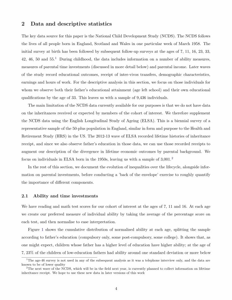
Figure 1 shows the cumulative distribution of normalised ability at each age, splitting the sample
according to father’s education (compulsory only, some post-compulsory, some college). It shows that, as
one might expect, children whose father has a higher level of education have higher ability; at the age of
7, 23% of the children of low-education fathers had ability around one standard deviation or more below
1The age-46 survey is not used in any of the subsequent analysis as it was a telephone interview only, and the data areknown to be of lower quality
2The next wave of the NCDS, which will be in the field next year, is currently planned to collect information on lifetimeinheritance receipt. We hope to use these new data in later versions of this work
4
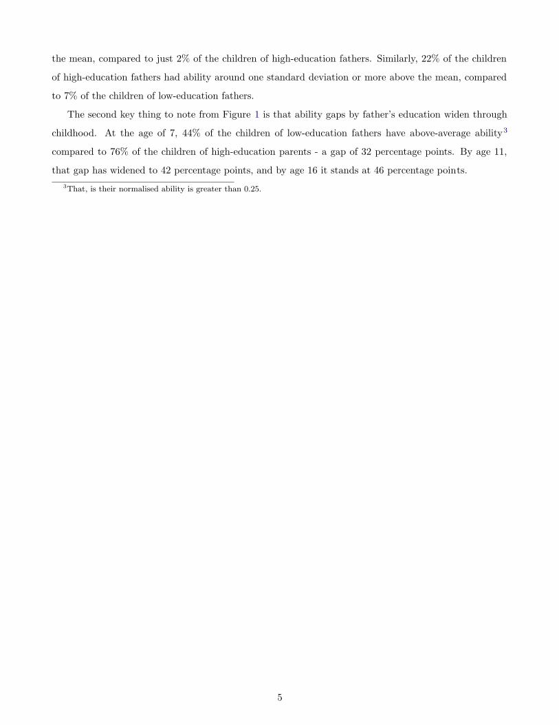
the mean, compared to just 2% of the children of high-education fathers. Similarly, 22% of the children
of high-education fathers had ability around one standard deviation or more above the mean, compared
to 7% of the children of low-education fathers.
The second key thing to note from Figure 1 is that ability gaps by father’s education widen through
childhood. At the age of 7, 44% of the children of low-education fathers have above-average ability3
compared to 76% of the children of high-education parents - a gap of 32 percentage points. By age 11,
that gap has widened to 42 percentage points, and by age 16 it stands at 46 percentage points.
3That, is their normalised ability is greater than 0.25.
5
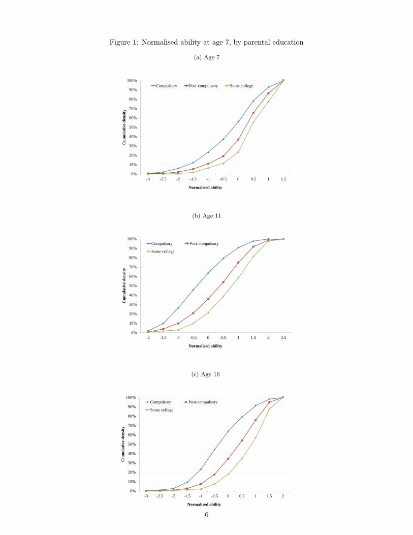
Figure 1: Normalised ability at age 7, by parental education
(a) Age 7
0%
10%
20%
30%
40%
50%
60%
70%
80%
90%
100%
-3 -2.5 -2 -1.5 -1 -0.5 0 0.5 1 1.5
Cu
mu
lati
ve d
ensi
ty
Normalised ability
Compulsory Post-compulsory Some college
(b) Age 11
0%
10%
20%
30%
40%
50%
60%
70%
80%
90%
100%
-2 -1.5 -1 -0.5 0 0.5 1 1.5 2 2.5
Cu
mu
lati
ve d
ensi
ty
Normalised ability
Compulsory Post-compulsory
Some college
(c) Age 16
0%
10%
20%
30%
40%
50%
60%
70%
80%
90%
100%
-3 -2.5 -2 -1.5 -1 -0.5 0 0.5 1 1.5 2
Cu
mu
lati
ve d
ensi
ty
Normalised ability
Compulsory Post-compulsory
Some college
6
Tables 1, 2 and 3 provide some descriptive evidence that at least some of the widening in ability
gaps by parental characteristics as children age can be explained by differential parental investments
(we investigate this hypothesis more formally in Section 3). Table 1 documents parental responses to
a question about reading with their child, asked when the child is 7. It shows relatively small but
potentially important differences in the frequency with which both mothers and fathers read to their
children, splitting families according to the education of the father. For example, 34% of fathers with
only compulsory education read to their 7-year-old children each week, compared to 53% of fathers with
some college education.
Tables 2 and 3 look at the child’s teachers assessment of parental interest in the child’s education, at
the ages of 7 and 11 respectively. The differences by father’s educational attainment are perhaps even
more striking than those in reading patterns. When the child is 7, fathers with some college education
are three times more likely to be judged by the teacher to be ‘very interested’ in their child’s education
as fathers with just compulsory education (62% compared to 21%). At the age of 11, the gap in paternal
interest is very similar, with 67% of college-educated fathers judged to be ‘very interested’ in their child’s
education, compared to 23% of fathers with just compulsory education. The Tables also show that having
a higher-educated father dramatically reduces the risk of a child having parents with little interest in
their education. Among those with a college-educated father, only 2-3% have a mother or father who is
judged to show ‘little interest’ in their education (at both ages). On the other hand, among those whose
father has only compulsory education that figure rises to 14-19%. It is an interesting empirical questions
whether parental characteristics matter more for the left or the right tail of the distribution of future
outcomes - do parents mainly insure children with low natural ability against bad outcomes, or are they
most important in ensuring children with high natural ability rise to the top?
Table 1: Frequency with which parents read to age-7 children
Father reads...Never Sometimes Every week
Father’s educationCompulsory 30% 36% 34%Post-compulsory 20% 35% 45%Some college 18% 29% 53%
Mother reads...Never Sometimes Every week
Father’s educationCompulsory 16% 37% 47%Post-compulsory 12% 31% 57%Some college 10% 23% 67%
7
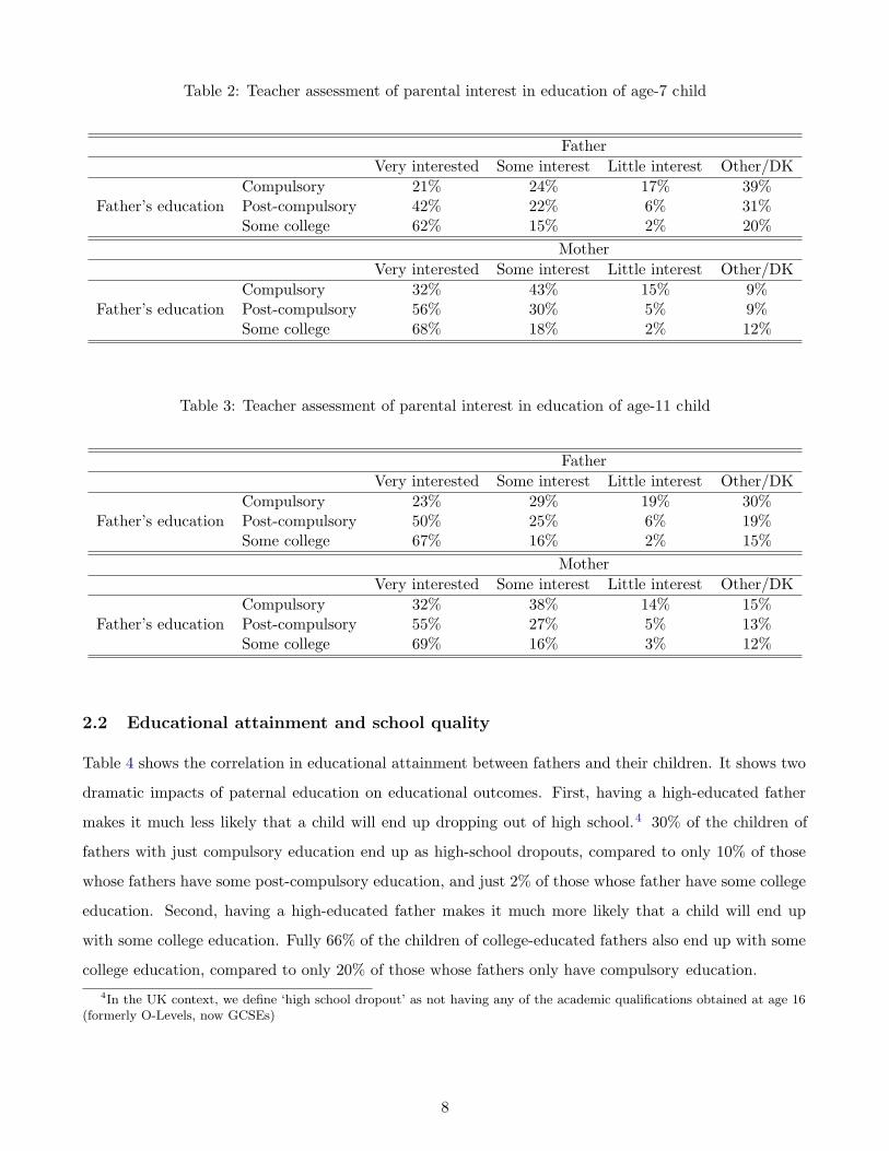
Table 2: Teacher assessment of parental interest in education of age-7 child
FatherVery interested Some interest Little interest Other/DK
Father’s educationCompulsory 21% 24% 17% 39%Post-compulsory 42% 22% 6% 31%Some college 62% 15% 2% 20%
MotherVery interested Some interest Little interest Other/DK
Father’s educationCompulsory 32% 43% 15% 9%Post-compulsory 56% 30% 5% 9%Some college 68% 18% 2% 12%
Table 3: Teacher assessment of parental interest in education of age-11 child
FatherVery interested Some interest Little interest Other/DK
Father’s educationCompulsory 23% 29% 19% 30%Post-compulsory 50% 25% 6% 19%Some college 67% 16% 2% 15%
MotherVery interested Some interest Little interest Other/DK
Father’s educationCompulsory 32% 38% 14% 15%Post-compulsory 55% 27% 5% 13%Some college 69% 16% 3% 12%
2.2 Educational attainment and school quality
Table 4 shows the correlation in educational attainment between fathers and their children. It shows two
dramatic impacts of paternal education on educational outcomes. First, having a high-educated father
makes it much less likely that a child will end up dropping out of high school.4 30% of the children of
fathers with just compulsory education end up as high-school dropouts, compared to only 10% of those
whose fathers have some post-compulsory education, and just 2% of those whose father have some college
education. Second, having a high-educated father makes it much more likely that a child will end up
with some college education. Fully 66% of the children of college-educated fathers also end up with some
college education, compared to only 20% of those whose fathers only have compulsory education.
4In the UK context, we define ‘high school dropout’ as not having any of the academic qualifications obtained at age 16(formerly O-Levels, now GCSEs)
8
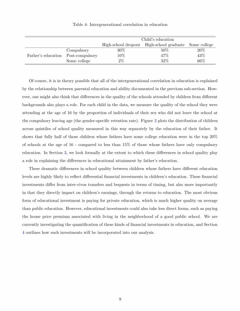
Table 4: Intergenerational correlation in education
Child’s educationHigh-school dropout High-school graduate Some college
Father’s educationCompulsory 30% 50% 20%Post-compulsory 10% 47% 43%Some college 2% 32% 66%
Of course, it is in theory possible that all of the intergenerational correlation in education is explained
by the relationship between parental education and ability documented in the previous sub-section. How-
ever, one might also think that differences in the quality of the schools attended by children from different
backgrounds also plays a role. For each child in the data, we measure the quality of the school they were
attending at the age of 16 by the proportion of individuals of their sex who did not leave the school at
the compulsory leaving age (the gender-specific retention rate). Figure 2 plots the distribution of children
across quintiles of school quality measured in this way separately by the education of their father. It
shows that fully half of those children whose fathers have some college education were in the top 20%
of schools at the age of 16 - compared to less than 15% of those whose fathers have only compulsory
education. In Section 3, we look formally at the extent to which these differences in school quality play
a role in explaining the differences in educational attainment by father’s education.
These dramatic differences in school quality between children whose fathers have different education
levels are highly likely to reflect differential financial investments in children’s education. These financial
investments differ from inter-vivos transfers and bequests in terms of timing, but also more importantly
in that they directly impact on children’s earnings, through the returns to education. The most obvious
form of educational investment is paying for private education, which is much higher quality on average
than public education. However, educational investments could also take less direct forms, such as paying
the house price premium associated with living in the neighborhood of a good public school. We are
currently investigating the quantification of these kinds of financial investments in education, and Section
4 outlines how such investments will be incorporated into our analysis.
9
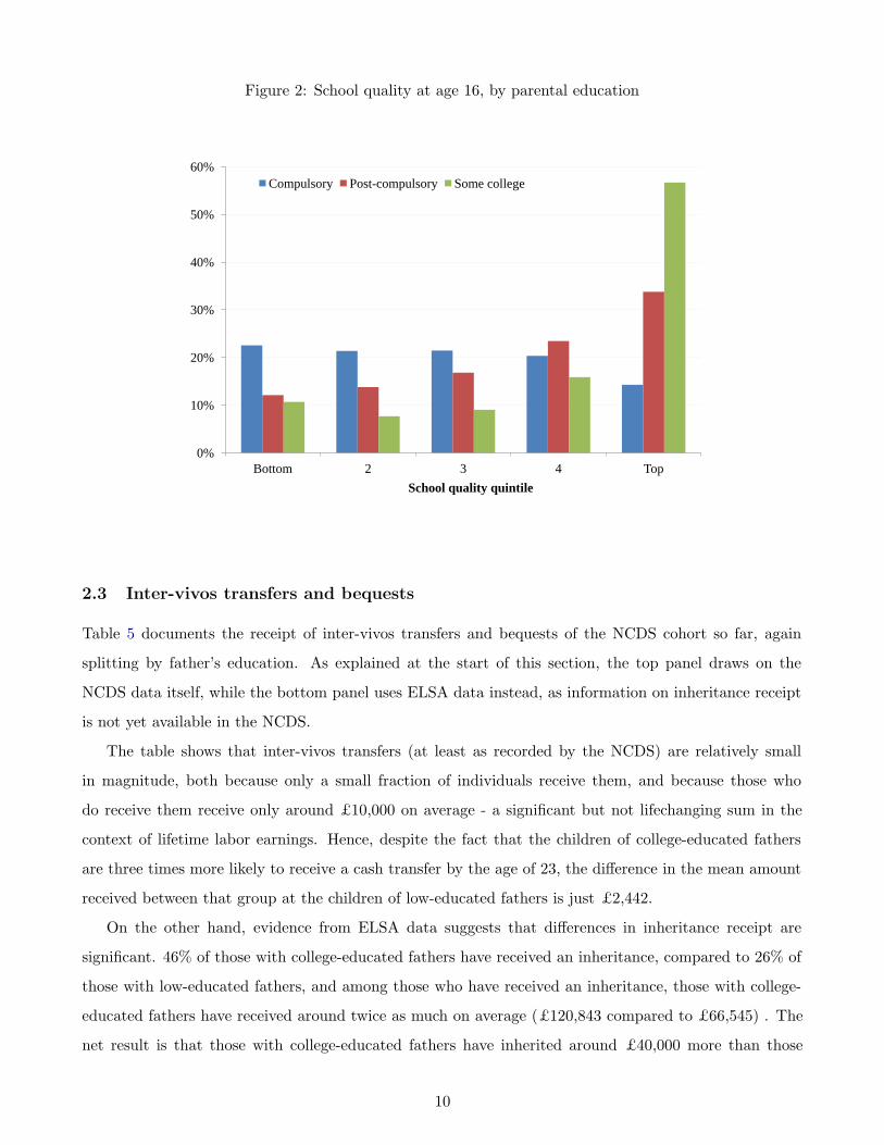
Figure 2: School quality at age 16, by parental education
0%
10%
20%
30%
40%
50%
60%
Bottom 2 3 4 Top
School quality quintile
Compulsory Post-compulsory Some college
2.3 Inter-vivos transfers and bequests
Table 5 documents the receipt of inter-vivos transfers and bequests of the NCDS cohort so far, again
splitting by father’s education. As explained at the start of this section, the top panel draws on the
NCDS data itself, while the bottom panel uses ELSA data instead, as information on inheritance receipt
is not yet available in the NCDS.
The table shows that inter-vivos transfers (at least as recorded by the NCDS) are relatively small
in magnitude, both because only a small fraction of individuals receive them, and because those who
do receive them receive only around £10,000 on average - a significant but not lifechanging sum in the
context of lifetime labor earnings. Hence, despite the fact that the children of college-educated fathers
are three times more likely to receive a cash transfer by the age of 23, the difference in the mean amount
received between that group at the children of low-educated fathers is just £2,442.
On the other hand, evidence from ELSA data suggests that differences in inheritance receipt are
significant. 46% of those with college-educated fathers have received an inheritance, compared to 26% of
those with low-educated fathers, and among those who have received an inheritance, those with college-
educated fathers have received around twice as much on average (£120,843 compared to £66,545) . The
net result is that those with college-educated fathers have inherited around £40,000 more than those
10
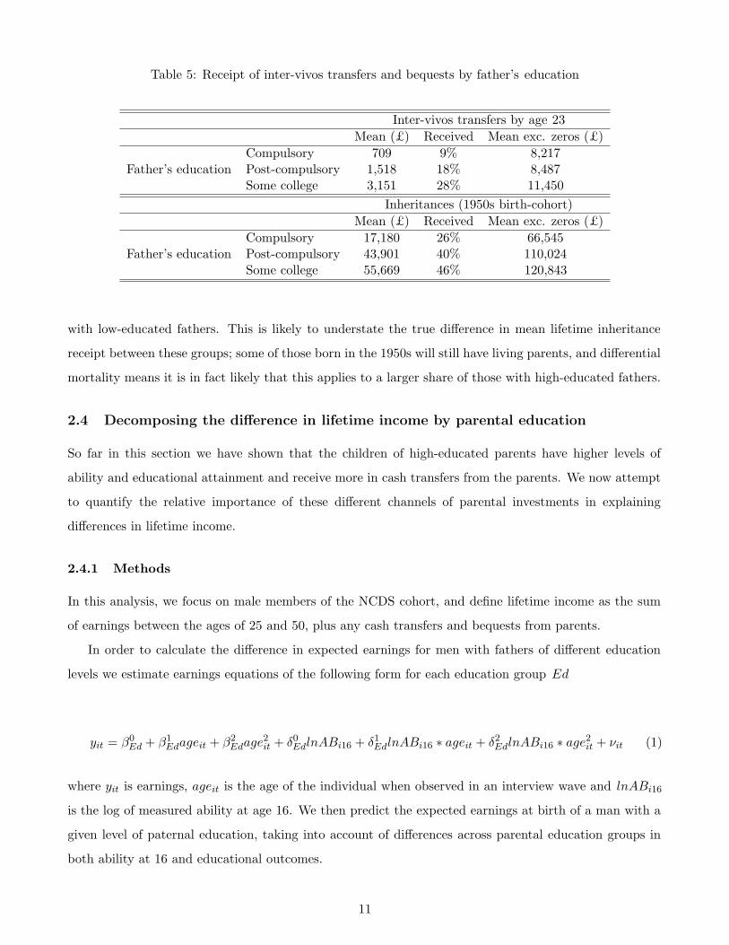
Table 5: Receipt of inter-vivos transfers and bequests by father’s education
Inter-vivos transfers by age 23Mean (£) Received Mean exc. zeros (£)
Father’s educationCompulsory 709 9% 8,217Post-compulsory 1,518 18% 8,487Some college 3,151 28% 11,450
Inheritances (1950s birth-cohort)Mean (£) Received Mean exc. zeros (£)
Father’s educationCompulsory 17,180 26% 66,545Post-compulsory 43,901 40% 110,024Some college 55,669 46% 120,843
with low-educated fathers. This is likely to understate the true difference in mean lifetime inheritance
receipt between these groups; some of those born in the 1950s will still have living parents, and differential
mortality means it is in fact likely that this applies to a larger share of those with high-educated fathers.
2.4 Decomposing the difference in lifetime income by parental education
So far in this section we have shown that the children of high-educated parents have higher levels of
ability and educational attainment and receive more in cash transfers from the parents. We now attempt
to quantify the relative importance of these different channels of parental investments in explaining
differences in lifetime income.
2.4.1 Methods
In this analysis, we focus on male members of the NCDS cohort, and define lifetime income as the sum
of earnings between the ages of 25 and 50, plus any cash transfers and bequests from parents.
In order to calculate the difference in expected earnings for men with fathers of different education
levels we estimate earnings equations of the following form for each education group Ed
yit = β0Ed + β1
Edageit + β2Edage2
it + δ0EdlnABi16 + δ1
EdlnABi16 ∗ ageit + δ2EdlnABi16 ∗ age2
it + νit (1)
where yit is earnings, ageit is the age of the individual when observed in an interview wave and lnABi16
is the log of measured ability at age 16. We then predict the expected earnings at birth of a man with a
given level of paternal education, taking into account of differences across parental education groups in
both ability at 16 and educational outcomes.
11
Having calculated expected earnings for each parental education group given the actual distributions
of ability and education within each group, we then do the same calculation for three counterfactual
distributions of ability and education across each paternal education group:
1. We predict the distribution of age-16 ability and education for each paternal education group con-
ditional on age-7 ability. Differences in expected earnings across groups in this scenario reveal how
much of observed differences in earnings by paternal education can be explained by the differences
in ability at age 7 shown in the first panel of Figure 1.
2. We predict the distribution of age-16 ability and education for each paternal education group condi-
tional on age-11 ability. The difference between expected earnings in this scenario and the previous
one captures the effects of the faster growth in ability between 7 and 11 for children of higher-
educated fathers.
3. We use the actual distribution of age-16 ability, but predict the education distribution for each group
on the basis of age-16 ability, ignoring other factors. The difference between expected earnings in
this scenario and the previous scenario captures the effects of the faster growth in ability between
11 and 16 for children of higher-educated fathers. The difference between expected earnings in
this scenario and true expected earnings captures the effect on lifetime earnings of other drivers of
educational outcomes besides ability (in our model, school quality).
2.4.2 Results
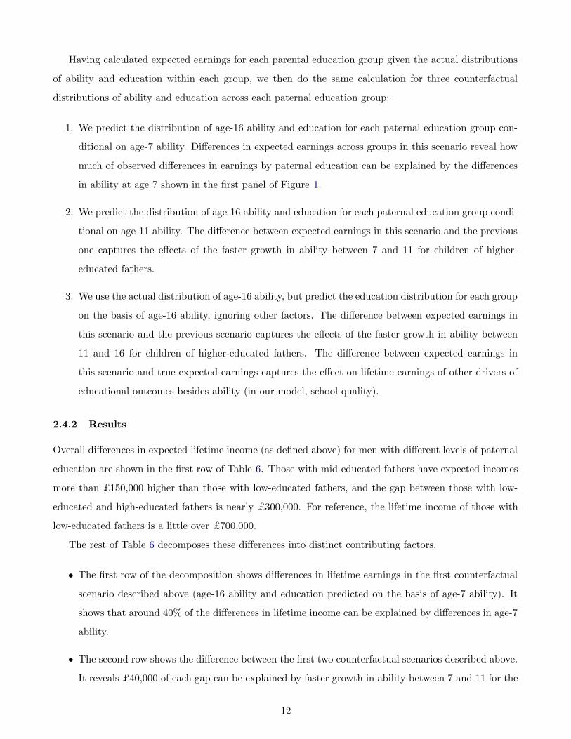
Overall differences in expected lifetime income (as defined above) for men with different levels of paternal
education are shown in the first row of Table 6. Those with mid-educated fathers have expected incomes
more than £150,000 higher than those with low-educated fathers, and the gap between those with low-
educated and high-educated fathers is nearly £300,000. For reference, the lifetime income of those with
low-educated fathers is a little over £700,000.
The rest of Table 6 decomposes these differences into distinct contributing factors.
• The first row of the decomposition shows differences in lifetime earnings in the first counterfactual
scenario described above (age-16 ability and education predicted on the basis of age-7 ability). It
shows that around 40% of the differences in lifetime income can be explained by differences in age-7
ability.
• The second row shows the difference between the first two counterfactual scenarios described above.
It reveals £40,000 of each gap can be explained by faster growth in ability between 7 and 11 for the
12
children of higher-educated parents. This is about 25% of the overall gap between the children of
low- and mid-educated fathers, and around 15% of the overall gap between the children of low- and
high-educated fathers.
• The third row shows the difference between the second and third counterfactual scenarios. The
different evolution of ability between 11 and 16 explains £11,000 (7%) of the difference in lifetime
incomes between children of low- and mid-educated fathers and £36,000 (11%) of the difference
between the chidren of low- and high-educated fathers.
• The fourth row shows the difference between the final counterfactual scenario and actual expected
earnings for each group. It suggests that differences in educational attainment conditional on ability
(explained by, for example, differences in school quality) explain more of the gap in income between
the children of low- and high-educated fathers (20%) than they explain of the gap between the sons
of low- and mid-educated fathers (10%).
• The final row of the Table simply documents differences in average inter-vivos transfers and bequests
across paternal education groups. It shows that around 15% of the differences in lifetime income
across these groups are attributable to differences in transfers and bequests, rather than differences
in earnings.
To summarise, the decomposition analysis suggests that around 40% of the difference in lifetime income
across paternal education groups is attributable to differences in ability at age 7, are explained by ability
at age 7, around 45% by subsequent divergence in ability and different educational outcomes, and around
15% by inter-vivos transfers and bequests received so far. Thus, while inter-vivos transfers are important,
most of the lifetime differences in lifetime income between children of low versus high education fathers
are realized by age 16.
3 Reduced-form evidence on the returns to parental investments
3.1 The effect of time investments on ability
In the previous section of the paper, we documented that the ability of children of higher-educated parents
rises faster through childhood than the ability of other children, and that their parents spent more time
reading to them and were more interested in their educational progress. We now look more formally at
the relationship between the those two facts using a simple regression framework.
To create a unidimensional measure of the time investments of parents in children (something that
is required for the model outlined in Section 4 to be tractable) we extract a principal component factor
13

Table 6: Decomposition of differences in lifetime income by father’s education
Father’s educationSome post-compulsory Some college
Total difference £159,000 £291,000
Explained by age-7 ability £65,000 £115,000Explained by evolution of ability 7-11 £42,000 £44,000Explained by evolution of ability 11-16 £11,000 £36,000Explained by school quality differences £17,000 £59,000Inter-vivos transfers and bequests £24,000 £37,000
Memo: Lifetime income for those with low-educated fathers: £736,000
Notes: Differences relative to those with low-educated fathers (compulsory education only). Figures calculated for men.
from our proxies for parental time investments. 5 For each age t = 7, 11 and t + 1 = 11, 16 we then run
the regression:
ABi,t+1 = ω + αABi,t + βTIi,t + δXit + uABit (2)
where AB is normalised ability, TI is our (normalised) measure of time investments (TI = TIm+TIf )
and X is a vector of background characteristics including parental education.
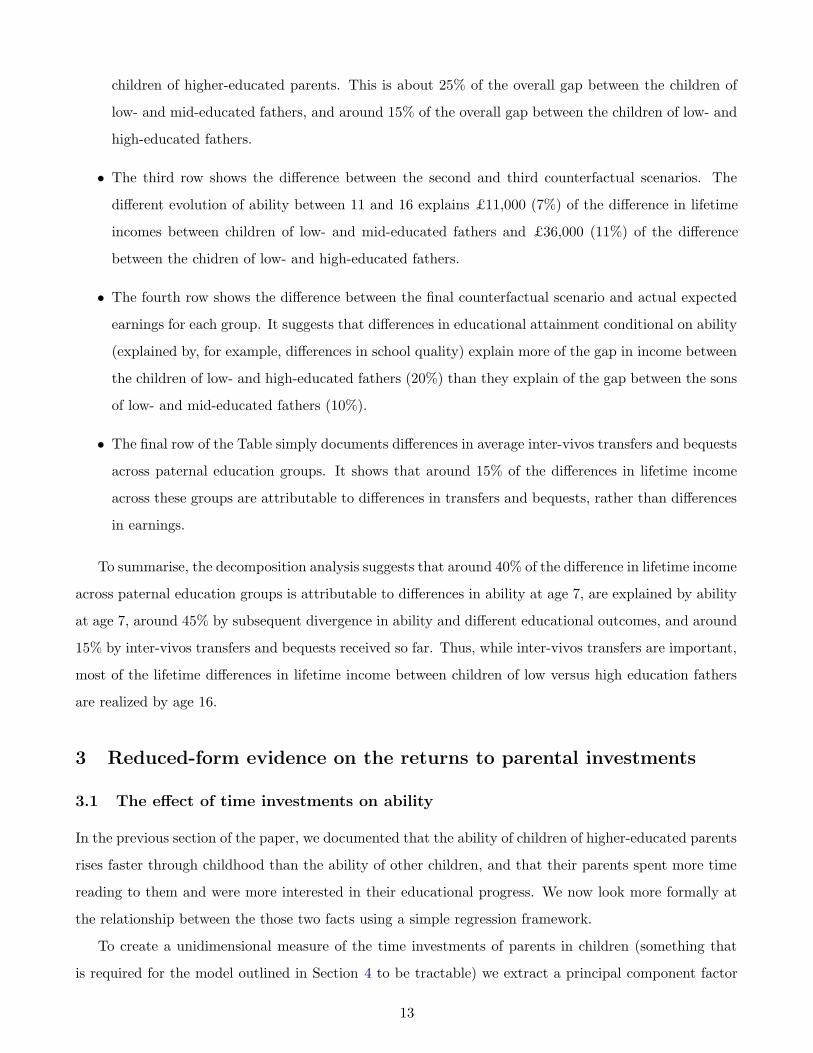
The results are presented in Table 7. It show that time investments have a significant effect on
changes in ability over time, even after conditioning on background characteristics. A one-standard
deviation increase in time investments at age 7 raises age-11 ability by 0.14 of a standard deviation, and
a one-standard deviation increase in time investments at age 11 raises age-16 ability by 0.09 of a standard
deviation.5At the age of 7, those proxies are frequency of reading with the child and interest in education. At the age of 11, the
proxies are interest in education and the number of educational activities (such as going to the library) the parents frequentlyengage in with the child.
14
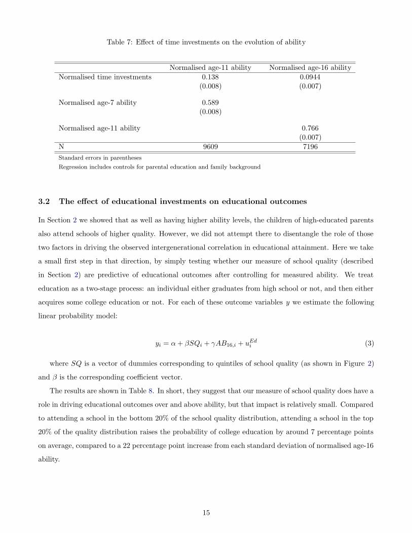
Table 7: Effect of time investments on the evolution of ability
Normalised age-11 ability Normalised age-16 abilityNormalised time investments 0.138 0.0944
(0.008) (0.007)
Normalised age-7 ability 0.589(0.008)
Normalised age-11 ability 0.766(0.007)
N 9609 7196
Standard errors in parentheses
Regression includes controls for parental education and family background
3.2 The effect of educational investments on educational outcomes
In Section 2 we showed that as well as having higher ability levels, the children of high-educated parents
also attend schools of higher quality. However, we did not attempt there to disentangle the role of those
two factors in driving the observed intergenerational correlation in educational attainment. Here we take
a small first step in that direction, by simply testing whether our measure of school quality (described
in Section 2) are predictive of educational outcomes after controlling for measured ability. We treat
education as a two-stage process: an individual either graduates from high school or not, and then either
acquires some college education or not. For each of these outcome variables y we estimate the following
linear probability model:
yi = α + βSQi + γAB16,i + uEdi (3)
where SQ is a vector of dummies corresponding to quintiles of school quality (as shown in Figure 2)
and β is the corresponding coefficient vector.
The results are shown in Table 8. In short, they suggest that our measure of school quality does have a
role in driving educational outcomes over and above ability, but that impact is relatively small. Compared
to attending a school in the bottom 20% of the school quality distribution, attending a school in the top
20% of the quality distribution raises the probability of college education by around 7 percentage points
on average, compared to a 22 percentage point increase from each standard deviation of normalised age-16
ability.
15
Table 8: Effect of ability and school quality on education
Complete HS Attend collegeNormalised age-16 ability 0.226 0.224
(0.005) (0.007)
School quality quintile=2 0.022 0.003(0.013) (0.019)
School quality quintile=3 0.028 0.005(0.013) (0.019)
School quality quintile=4 0.046 0.040(0.013) (0.018)
School quality quintile=5 0.018 0.070(0.014) (0.019)
Constant 0.731 0.252(0.009) (0.014)
N 7803 6070
Standard errors in parentheses
Results from linear probability model. Excluded category is bottom quintile of school quality.
HS dropouts not included in college regression.
4 Model
This section gives an outline of a dynamic model of consumption and labor supply in which parents
can make different types of transfers to their children. The model can be used to a) evaluate how
particular intergenerational transfers affect household behavior, b) compare the relative insurance value
of these types of transfers and c) simulate household behavior and welfare under counterfactual policies
(for example, under reforms to estate taxation).
Before detailing the model we provide a short summary of its key features. An individual’s lifecycle
is split into four phases: i) the ‘child phase’, up to the age of 16, during which decisions are taken on
their behalf by their parents, ii) the ‘growing-up phase’, between the ages of 16 and 23, when individuals’
educational outcomes are realised and they form couples, iii) the ‘early adult phase’, from the age of 23
to 46 when couples make decisions as a collective unit and have a dependent child, and iv) the ‘late adult’
phase, from the age of 46, after their child has grown up, when couples are subject to stochastic mortality
risk.
16

4.1 Timing and Notation
In outlining the model we describe below a lifecycle decision problem of a couple belonging to single
generation. All generations are, of course, linked – each member of the couple whose decision problem we
specify has parents, and they, in turn, will have children. We will refer to the generation whose problem
we outline as generation 1, their parents as generation 0, and their children as generation 2. In the
exposition below, model periods are indexed by the age of the members of the couples in generation 1.6
4.2 Utility
Utility of each member of the couple g ∈ {m, f} (male and female respectively) depends on their con-
sumption and leisure:
ug(c, l) =(cνg l(1−νg))1−γ
1 − γ
We assume full consumption sharing between spouses:
cm = cf = 0.5c
where c is household consumption. Household preferences are given by the sum of male and female utility.
u(c, lm, lf ) = um(cm, lm) + uf (cf , lf )
4.3 Decision and constraints in each phase of life
4.3.1 Child phase
Decisions During this phase, generation 1 are children and are not making any decisions on their own
behalf. Parents (generation 0), who are in the ‘early adult’ phase of life. We describe here the decision
problem of those parents. They make up to four choices each period. These are (with the time periods
in which those decisions are taken given in parentheses):
1. Household consumption – c0 (each period)
2. Hours of work for each parent – hm,0, hf,0 where m and f index hours of work by the male and
female respectively (each period)
3. Time investments in children – TI0 (at ages up to age 11)
4. Money investments in children’s education – MI0 (only at age 11)6That is, subscripts are an index of calendar time, not of age. For example, V 1
50() is the value function of generation 1 atthe age of 50, but V 2
50() is the value function of generation 2 in the year that generation 2 was 50 years old.
17
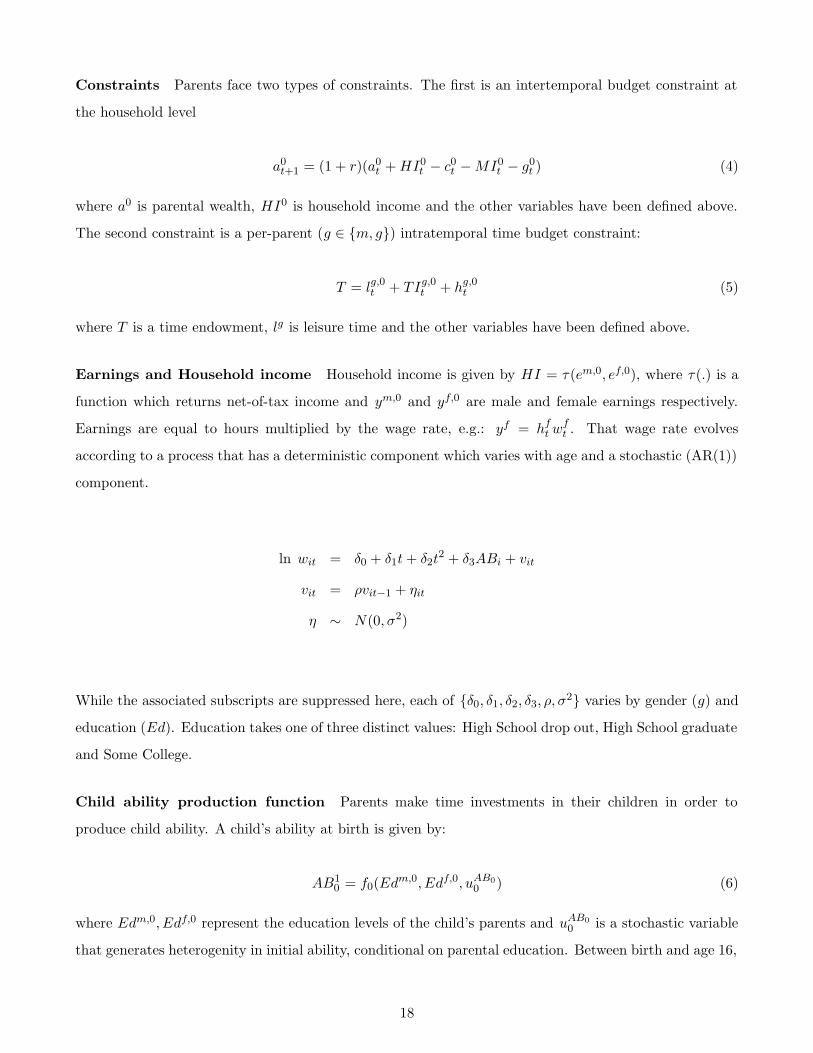
Constraints Parents face two types of constraints. The first is an intertemporal budget constraint at
the household level
a0t+1 = (1 + r)(a0
t + HI0t − c0
t − MI0t − g0
t ) (4)
where a0 is parental wealth, HI0 is household income and the other variables have been defined above.
The second constraint is a per-parent (g ∈ {m, g}) intratemporal time budget constraint:
T = lg,0t + TIg,0
t + hg,0t (5)
where T is a time endowment, lg is leisure time and the other variables have been defined above.
Earnings and Household income Household income is given by HI = τ(em,0, ef,0), where τ(.) is a
function which returns net-of-tax income and ym,0 and yf,0 are male and female earnings respectively.
Earnings are equal to hours multiplied by the wage rate, e.g.: yf = hft wf
t . That wage rate evolves
according to a process that has a deterministic component which varies with age and a stochastic (AR(1))
component.
ln wit = δ0 + δ1t + δ2t2 + δ3ABi + vit
vit = ρvit−1 + ηit
η ∼ N(0, σ2)
While the associated subscripts are suppressed here, each of {δ0, δ1, δ2, δ3, ρ, σ2} varies by gender (g) and
education (Ed). Education takes one of three distinct values: High School drop out, High School graduate
and Some College.
Child ability production function Parents make time investments in their children in order to
produce child ability. A child’s ability at birth is given by:
AB10 = f0(Edm,0, Edf,0, uAB0
0 ) (6)
where Edm,0, Edf,0 represent the education levels of the child’s parents and uAB00 is a stochastic variable
that generates heterogenity in initial ability, conditional on parental education. Between birth and age 16,
18
child ability updates each period. The accumulation equation depends on ability in the previous period,
parental education, time investments by both parents and a stochastic innovation.
AB1t+1 = f(ABt, Edm,0, Edf,0, T If
t , T Ift , uAB
t+1)
Ability evolves until the age of 16, after which it is an absorbing state.
School quality production function School quality will be an input into the child’s educational
attainment which will be realised during the ‘growing-up’ phase of life. A child’s school quality (SQ1) is
determined at the age of 16. It depends on their ability at the age of 11, their parents’ education, money
investments their parents’ choose to make and a stochastic component (uSQ).
SQ1 = h(AB111, Edm,0, Edf,0,MI0
11, uSQ) (7)
4.3.2 Growing-up phase
Children ‘grow up’ between the ages of 16 – the last modeled child period – and 23 – the first modeled
adult period.7 During this phase, the parents remain the decision-maker, and their choice variables are:
1. Household consumption
2. Hours of work for each parent
3. A cash gift (g0) to their children. This gift represents inter-vivos transfers and inheritances.
Additionally, in this phase, after those decisions are made, two distinct changes occur to the child:
1. Their education is realised. It depends on a child’s ability, their school quality and a stochastic
variable (uEd1).
Ed1 = g(AB116, SQ1, uEd1
)
2. Couples are formed on the basis of a matching function which depends on education. Each new
couple gives birth to a child of their own.
7This represents only one modelled period - we model decisions as taking place at the ages ( t) of 7, 11, 16, 23, 33, 42, 50,55, 60 (and at five-yearly intervals after the age of 60). These ages are chosen to align with the ages at which the respondentsto the survey which is our primary data source are sampled. The model periods should be thought of as representing theages up to and including that period (that is period 7 represent decisions taken between birth and 7, period 11 accounts fordecisions taken between the ages of 8 and 11 etc.).
19
4.3.3 Early Adult phase
From the age of 23, generation 1 (now in couples) start to make their own decisions: over household
labor supply, consumption, and investments (time and money) in their children (generation 2). Their
decision problem in this phase has already been outlined – in Sections 4.3.1 and 4.3.2 – which describe
the decisions of the parents of generation 1 when the latter were in, respectively, the child phase and
growing-up phase.
4.3.4 Late Adult phase
At the age of 46, the children of generation 1 (i.e., the members of generation 2) enter their own early
adult phase and the generation 1 couple enters a ‘late adult phase’, during which they make labor supply
and consumption/saving decisions only. There is stochastic mortality (where assume that both members
of the couple die in the same period).
4.4 Discounting and intergenerational altruism
In discounting their future utility each generation applies a geometric discount factor (β). Each generation
is altruistic regarding the utility of their offspring (and indeed future generations). In addition to the
time discounting of their children’s future utility, they additionally discount it with an intergenerational
altruism parameter (λ).
4.5 State Variables
The vector of state variables (X1,e) during the early adult phase of life contains (for generation 1):
1. Age (t)
2. Assets (A1)
3. Wage rates (wm,1, wf,1)
4. Eduction levels (Edm,1, Edf,1)
5. Own abilities (ABm,1, ABf,1)
6. Child’s ability (AB2)
The vector state variables (X1,l) during the late adult phase of life are the same as those for the early
adult phase except that the (now-grown-up child’s ability is no longer a state variable):
20
1. Age (t)
2. Assets (A1)
3. Wage rates (wm,1, wf,1)
4. Eduction levels (Edm,1, Edf,1)
5. Own abilities (ABm,1, ABf,1)
4.6 Value Functions and Formal Expression of Decision Problem
In this section we formally outline the value functions and give a formal expression of the decision problem.
Expressing the problem for generation 1, we first give the late adult phase (when generation 2 have grown
up), second we give the value function for the last period of early adulthood (when generation two are in
the growing up phase) and finally give the value function for the rest of early adulthood (when generation
two are children).
4.6.1 Late adult
In the ‘late adult’ phase of life, households make choices over labor supply and consumption, and there
is uncertainty over mortality and the innovation to each spouse’s wage equation. The joint distribution
of these stochastic variables (ql ≡ {ηm, ηf} is given by Fl(ql). The decision problem in the ‘late adult’
phase of life can be expressed as:
V 1,lt (X1,l
t ) = maxc1t ,hm,1,hf,1
(
u(ct, lmt , lft ) + βst+1
∫V 1,l
t+1(X1,lt+1)dFl(q
l)
)
(8)
s.t. the intertemporal budget constraint in equation (4)
and the time budget constraint in equation (5)
where st+1 is the probability of surviving to period t + 1, conditional on having survived to period t.
4.6.2 Last period in early adult phase
The decision problem of generation 1 in the last period of the early adult phase of life (the period that
their children are in the ‘growing-up’ phase of life) is:
21
V 1,et (X1,e
t ) = maxc1t ,hm,1,hf,1,g1
(
u(ct, lmt , lft ) +β
∫V 1,l
t+1(X1,lt+1)dF (q) (9)
+βλ
∫V 2,e
t+1(X2,et+1)dG(Q)
)
s.t. the intertemporal budget constraint in equation (4)
and the time budget constraint in equation (5)
Note that there are two continuation value functions here. The first is the future expected utility of
that the decision-making couple will enjoy in the next period (when they will enter late-adulthood). The
value function (given in equation 8) must be integrated with respect to next period’s wage draws, which
are stochastic, and discounted by β, the time discount factor. The second continuation value function
is the expected value of the couple to which the child of the generation 1 decision-maker will belong
to. The (altruistic) parents take this into account in making their decisions. This continuation utility is
discounted by both the time discount factor and the altruism parameter (λ). This value function is the
early adult value function for generation 2 (the early adult value function will be given below). 8 This must
be integrated over those attributes of the couples’ children which will be realised during the ‘growing-up’
phrase (their education and initial wage draw) and the attributes of their future spouse – his/her ability,
education level, assets, and initial wage draw. The stochastic variables are collected in a vector Q, and
their joint distribution is given by G().
4.6.3 Other periods in early adult phase)
In the early years of being an adult, households face make choices over consumption, labor supply, and
investments of time and money in their children. They face uncertainty over the innovation to their
wage equation, and over the stochastic innovations to the child ability production function and the school
quality production function. The joint distribution of these stochastic variables (qe ≡ {ηm, ηf , uAB , uSQ}
is given by Fe(qe). The decision problem for each period in this phase – which starts as the new couple
becoming the decision-maker (at age 23) and which ends in the penultimate period in the early adult
phase is given below.
8Recall that the timing convention that we index all value functions in this exposition by the age of generation 1. Thatis, V 2,e
t+1 is the value function for generation 2 when generation 1 is aged t + 1.
22
V 1,et (X1,e
t ) = maxc1t ,hm,1,hf,1,T I1,MI1
(
u(ct, lmt , lft ) + β
∫V 1,e
t+1(X1,et+1)dFe(q
e) (10)
s.t. the intertemporal budget constraint in equation (4)
and the time budget constraint in equation (5)
5 Conclusions and policy implications
Understanding intergenerational links, and in particular the role of parental investments, is crucial for
policymakers seeking to design redistributive tax and transfer policies that mitigate inequalities and
improve social mobility. In this paper we have documented substantial differences between children
from different backgrounds in the evolution of cognitive ability through childhood, school quality and
educational outcomes, and cash transfers received from their parents. A quantification of the implications
of this differences for lifetime incomes suggests that around 40% of the gap between the sons of low- and
high-educated fathers can be attributed to ability differences at the age of 7, a further 45% to subsequent
differences in ability and educational attainment, and the final 15% to differences in the amount of inter-
vivos transfers and bequests received. We provide evidence that at least some of the differences in ability
and education are attributable to parental time investments in children and investments in school quality
respectively. Finally, we outline a model that captures all three investment channels and will allow analysis
of counterfactual polices that incorporates household’s responses.
All this has a number of implications for economic policy. At the most general level, the paper
shows that policymakers interested in tackling the intergenerational transmission of inequalities need to
consider policies designed to counter the inequality-increasing effects of each of the three forms of parental
investment, since each proves to be quantitatively important in driving inequalities in income. Moreover,
policymakers should bear in mind the substitutability of these different forms of investment - any attempt
to shut down one channel of parental investments is likely to provoke a shift towards investment in
other forms. In fact, the elasticity of substitution between these different forms of investment is a key
determinant of the optimal policy response.
The findings of this paper also have a number of more specific implications for tax and transfer policies.
First, redistributive transfer programs are often explicitly justified as providing insurance against certain
kinds of shocks, such as health or unemployment shocks. The findings of this paper suggest that a possible
justification for means-tested programs that seem to have less of an insurance role (such as EITC) is that
they provide insurance against parental characteristics, which are an uninsurable risk from the perspective
of the child. Second, the role of earnings replacement in old-age pensions should be considered in light of
23
the positive correlation between earnings and the receipt of cash transfers and bequests from parents. In
short, if higher earners are more likely to see their retirement resources supplemented by transfers from
parents, is it desirable for the state to also provide more money to such individuals in retirement to the
extent that is currently the case? Third, the role of cash transfers from parents should feature in an
assessment of the role of asset contigency in welfare and social security programs. In a world in which all
wealth is lifecycle wealth accumulated from past labor earnings, restricting access to state support on the
basis of assets acts as a disincentive to work. However, to the extent that assets are not accumulated from
labor earnings but transferred from parents, making programs asset-contingent becomes a more attractive
way to target them on the desired recipients.
References
Abbott, B., G. Gallipoli, C. Meghir, and G. Violante (2016). Education policy and intergenerational
transfers in equilibrium. Technical report, Cowles Foundation Discussion paper.
Charles, K. K. and E. Hurst (2003). The correlation of wealth across generations. Journal of Political
Economy 111 (6), 1155–1182.
Chetty, R., N. Hendren, P. Kline, and E. Saez (2014). Where is the land of opportunity: The geography
of intergenerational mobility in the united states. Quarterly Journal of Economics 129 (4), 1553–1623.
De Nardi, M. (2004). Wealth inequality and intergenerational links. The Review of Economic Stud-
ies 71 (3), pp. 743–768.
Del Boca, D., C. Flinn, and M. Wiswall (2014). Household choices and child development. The Review
of Economic Studies 81 (1), 137.
Gayle, G.-L., L. Golan, and M. Soytas (2015). What is the source of the intergenerational correlation in
earnings. Technical report, Mimeo.
24


