Download - TUTORIAL IN BIOSTATISTICS META-ANALYSIS: FORMULATING, EVALUATING ... · META-ANALYSIS: FORMULATING, EVALUATING, COMBINING, AND REPORTING ... a tutorial on meta-analysis intended for

STATISTICS IN MEDICINEStatist. Med. 18, 321–359 (1999)

TUTORIAL IN BIOSTATISTICSMETA-ANALYSIS: FORMULATING, EVALUATING,

COMBINING, AND REPORTING

SHARON-LISE T. NORMAND ∗

Department of Health Care Policy, Harvard Medical School, 180 Longwood Avenue, Boston, MA 02115, U.S.A., andDepartment of Biostatistics, Harvard School of Public Health, 677 Huntington Avenue, Boston, MA 02115, U.S.A.

SUMMARY

Meta-analysis involves combining summary information from related but independent studies. The objectivesof a meta-analysis include increasing power to detect an overall treatment e!ect, estimation of the degree ofbene"t associated with a particular study treatment, assessment of the amount of variability between studies,or identi"cation of study characteristics associated with particularly e!ective treatments. This article presentsa tutorial on meta-analysis intended for anyone with a mathematical statistics background. Search strategiesand review methods of the literature are discussed. Emphasis is focused on analytic methods for estimation ofthe parameters of interest. Three modes of inference are discussed: maximum likelihood; restricted maximumlikelihood, and Bayesian. Finally, software for performing inference using restricted maximum likelihoodand fully Bayesian methods are demonstrated. Methods are illustrated using two examples: an evaluation ofmortality from prophylactic use of lidocaine after a heart attack, and a comparison of length of hospital stayfor stroke patients under two di!erent management protocols. Copyright ? 1999 John Wiley & Sons, Ltd.

1. INTRODUCTION

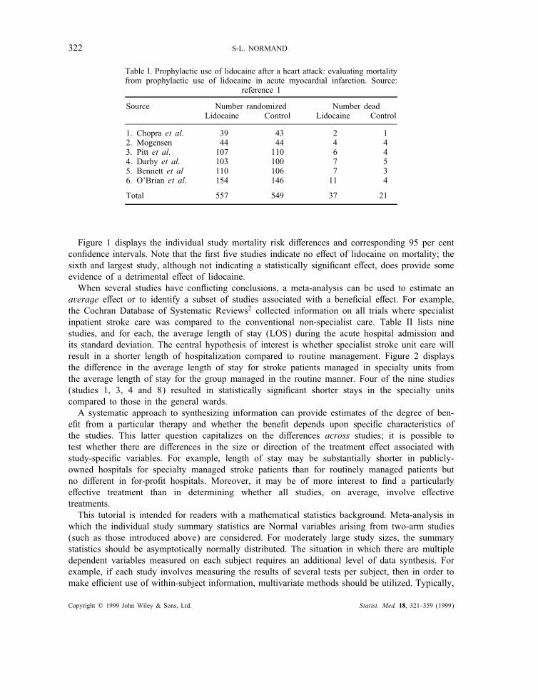
Meta-analysis may be broadly de"ned as the quantitative review and synthesis of the resultsof related but independent studies. The objectives of a meta-analysis can be several-fold. Bycombining information over di!erent studies, an integrated analysis will have more statisticalpower to detect a treatment e!ect than an analysis based on only one study. For example, Hineet al.1 conducted a meta-analysis of death rates in randomized controlled trials in which prophy-lactic lidocaine was administered to patients with proved or suspected acute myocardial infarction.Table I describes mortality at the end of the assigned treatment period for control and intravenouslidocaine treatment groups for six studies. The unadjusted total mortality rates were 6·6 per cent(37=557) in the lidocaine group and 3·8 per cent (21=549) in the control group. The question ofinterest is whether there is a detrimental e!ect of lidocaine. Because the studies were conductedto compare rates of arrhythmias following a heart attack, the studies, taken individually, are toosmall to detect important di!erences in mortality rates.

∗ Correspondence to: Sharon-Lise T. Normand, Department of Health Care Policy, Harvard Medical School, 180 LongwoodAvenue, Boston MA 02115, U.S.A.

Contract=grant sponsor: National Cancer InstituteContract=grant number: CA-61141

CCC 0277–6715/99/030321–39 $17.50 Received January 1998Copyright ? 1999 John Wiley & Sons, Ltd. Accepted April 1998

322 S-L. NORMAND

Table I. Prophylactic use of lidocaine after a heart attack: evaluating mortalityfrom prophylactic use of lidocaine in acute myocardial infarction. Source:

reference 1

Source Number randomized Number deadLidocaine Control Lidocaine Control

1. Chopra et al. 39 43 2 12. Mogensen 44 44 4 43. Pitt et al. 107 110 6 44. Darby et al. 103 100 7 55. Bennett et al 110 106 7 36. O’Brian et al. 154 146 11 4

Total 557 549 37 21

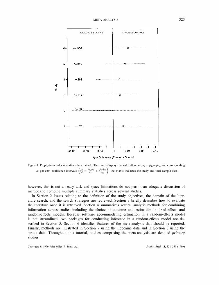
Figure 1 displays the individual study mortality risk di!erences and corresponding 95 per centcon"dence intervals. Note that the "rst "ve studies indicate no e!ect of lidocaine on mortality; thesixth and largest study, although not indicating a statistically signi"cant e!ect, does provide someevidence of a detrimental e!ect of lidocaine.When several studies have con#icting conclusions, a meta-analysis can be used to estimate an

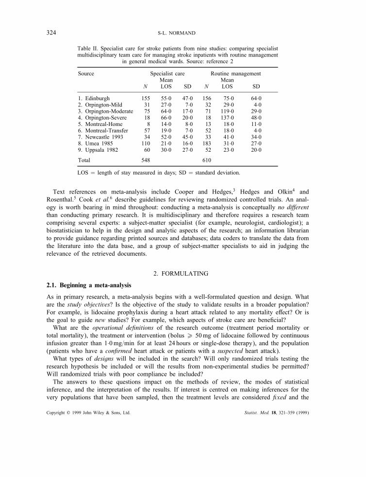
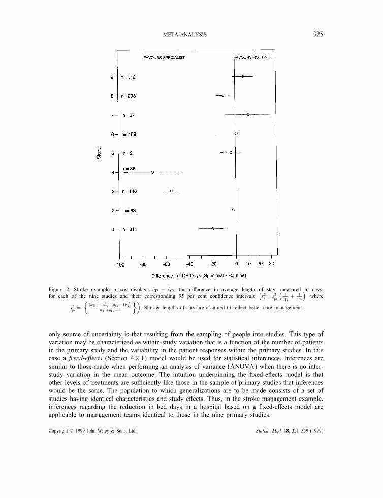
average e!ect or to identify a subset of studies associated with a bene"cial e!ect. For example,the Cochran Database of Systematic Reviews2 collected information on all trials where specialistinpatient stroke care was compared to the conventional non-specialist care. Table II lists ninestudies, and for each, the average length of stay (LOS) during the acute hospital admission andits standard deviation. The central hypothesis of interest is whether specialist stroke unit care willresult in a shorter length of hospitalization compared to routine management. Figure 2 displaysthe di!erence in the average length of stay for stroke patients managed in specialty units fromthe average length of stay for the group managed in the routine manner. Four of the nine studies(studies 1, 3, 4 and 8) resulted in statistically signi"cant shorter stays in the specialty unitscompared to those in the general wards.A systematic approach to synthesizing information can provide estimates of the degree of ben-

e"t from a particular therapy and whether the bene"t depends upon speci"c characteristics ofthe studies. This latter question capitalizes on the di!erences across studies; it is possible totest whether there are di!erences in the size or direction of the treatment e!ect associated withstudy-speci"c variables. For example, length of stay may be substantially shorter in publicly-owned hospitals for specialty managed stroke patients than for routinely managed patients butno di!erent in for-pro"t hospitals. Moreover, it may be of more interest to "nd a particularlye!ective treatment than in determining whether all studies, on average, involve e!ectivetreatments.This tutorial is intended for readers with a mathematical statistics background. Meta-analysis in

which the individual study summary statistics are Normal variables arising from two-arm studies(such as those introduced above) are considered. For moderately large study sizes, the summarystatistics should be asymptotically normally distributed. The situation in which there are multipledependent variables measured on each subject requires an additional level of data synthesis. Forexample, if each study involves measuring the results of several tests per subject, then in order tomake e$cient use of within-subject information, multivariate methods should be utilized. Typically,

Copyright ? 1999 John Wiley & Sons, Ltd. Statist. Med. 18, 321–359 (1999)

META-ANALYSIS 323

Figure 1. Prophylactic lidocaine after a heart attack. The x-axis displays the risk di!erence, di = pTi−pCi , and corresponding

95 per cent con"dence intervals(

s2di =pTi qTinTi

+ pCi qCinCi

)

; the y-axis indicates the study and total sample size

however, this is not an easy task and space limitations do not permit an adequate discussion ofmethods to combine multiple summary statistics across several studies.In Section 2 issues relating to the de"nition of the study objectives, the domain of the liter-

ature search, and the search strategies are reviewed. Section 3 brie#y describes how to evaluatethe literature once it is retrieved. Section 4 summarizes several analytic methods for combininginformation across studies including the choice of outcome and estimation in "xed-e!ects andrandom-e!ects models. Because software accommodating estimation in a random-e!ects modelis not streamlined, two packages for conducting inference in a random-e!ects model are de-scribed in Section 5. Section 6 identi"es features of the meta-analysis that should be reported.Finally, methods are illustrated in Section 7 using the lidocaine data and in Section 8 using thestroke data. Throughout this tutorial, studies comprising the meta-analysis are denoted primarystudies.


324 S-L. NORMAND

Table II. Specialist care for stroke patients from nine studies: comparing specialistmultidisciplinary team care for managing stroke inpatients with routine management

in general medical wards. Source: reference 2

Source Specialist care Routine managementMean Mean

N LOS SD N LOS SD

1. Edinburgh 155 55·0 47·0 156 75·0 64·02. Orpington-Mild 31 27·0 7·0 32 29·0 4·03. Orpington-Moderate 75 64·0 17·0 71 119·0 29·04. Orpington-Severe 18 66·0 20·0 18 137·0 48·05. Montreal-Home 8 14·0 8·0 13 18·0 11·06. Montreal-Transfer 57 19·0 7·0 52 18·0 4·07. Newcastle 1993 34 52·0 45·0 33 41·0 34·08. Umea 1985 110 21·0 16·0 183 31·0 27·09. Uppsala 1982 60 30·0 27·0 52 23·0 20·0

Total 548 610

LOS = length of stay measured in days; SD = standard deviation.

Text references on meta-analysis include Cooper and Hedges,3 Hedges and Olkin4 andRosenthal.5 Cook et al.6 describe guidelines for reviewing randomized controlled trials. An anal-ogy is worth bearing in mind throughout: conducting a meta-analysis is conceptually no di!erentthan conducting primary research. It is multidisciplinary and therefore requires a research teamcomprising several experts: a subject-matter specialist (for example, neurologist, cardiologist); abiostatistician to help in the design and analytic aspects of the research; an information librarianto provide guidance regarding printed sources and databases; data coders to translate the data fromthe literature into the data base, and a group of subject-matter specialists to aid in judging therelevance of the retrieved documents.

2. FORMULATING

2.1. Beginning a meta-analysis

As in primary research, a meta-analysis begins with a well-formulated question and design. Whatare the study objectives? Is the objective of the study to validate results in a broader population?For example, is lidocaine prophylaxis during a heart attack related to any mortality e!ect? Or isthe goal to guide new studies? For example, which aspects of stroke care are bene"cial?What are the operational de"nitions of the research outcome (treatment period mortality or

total mortality), the treatment or intervention (bolus ¿ 50mg of lidocaine followed by continuousinfusion greater than 1·0mg=min for at least 24 hours or single-dose therapy), and the population(patients who have a con"rmed heart attack or patients with a suspected heart attack).What types of designs will be included in the search? Will only randomized trials testing the

research hypothesis be included or will the results from non-experimental studies be permitted?Will randomized trials with poor compliance be included?The answers to these questions impact on the methods of review, the modes of statistical

inference, and the interpretation of the results. If interest is centred on making inferences for thevery populations that have been sampled, then the treatment levels are considered "xed and the


META-ANALYSIS 325

Figure 2. Stroke example. x-axis displays %xTi − %xCi , the di!erence in average length of stay, measured in days,for each of the nine studies and their corresponding 95 per cent con"dence intervals

(

s2i = s2pi

(

1nTi+ 1

nCi

)

where

s2pi ={

(nTi−1)s2Ti+(nCi−1)s2Ci

n Ti+nCi−2

})

. Shorter lengths of stay are assumed to re#ect better care management

only source of uncertainty is that resulting from the sampling of people into studies. This type ofvariation may be characterized as within-study variation that is a function of the number of patientsin the primary study and the variability in the patient responses within the primary studies. In thiscase a "xed-e!ects (Section 4.2.1) model would be used for statistical inferences. Inferences aresimilar to those made when performing an analysis of variance (ANOVA) when there is no inter-study variation in the mean outcome. The intuition underpinning the "xed-e!ects model is thatother levels of treatments are su$ciently like those in the sample of primary studies that inferenceswould be the same. The population to which generalizations are to be made consists of a set ofstudies having identical characteristics and study e!ects. Thus, in the stroke management example,inferences regarding the reduction in bed days in a hospital based on a "xed-e!ects model areapplicable to management teams identical to those in the nine primary studies.


326 S-L. NORMAND

On the other hand, if inferences are to be generalized to a population in which the studies arepermitted to have di!erent e!ects and di!erent characteristics, then a random-e!ects (Section 4.2.2)model would be appropriate. The intuition underpinning random-e!ects models is that because thereare many di!erent approaches to conducting a study by perturbing the design in a small way, thenthere are many di!erent potential treatment e!ects that could arise. This situation corresponds toan ANOVA model in which there is inter-study variation in the mean outcome in addition to thewithin-study variation. Thus, the population in a random-e!ects model is the one in which thereare in"nitely many possible populations. Inferences regarding the e!ect of lidocaine based on arandom-e!ects model applies to the population that would be formed if additional studies weresampled in a manner similar to that used to obtain the six primary studies.There are conceptual di$culties linked to both the "xed-e!ects and random-e!ects points of

view. In both models, it may be di$cult to characterize precisely the universe to which we areinferring. In the random-e!ects model, the universe may too big to imagine and in the "xed-e!ectsmodel, too small to be of any practical importance. There is a long debate as to the choice ofappropriate model that cannot be adequately covered in this tutorial. What should be noted isthat it is almost always reasonable to believe that there is some between-study variation and fewreasons to believe it is zero. However, if all the lidocaine studies indicate that lidocaine is relatedto increased mortality then it may be of little concern that some studies favour it more stronglythan others. On the other hand, when studies con#ict, such as in the stroke example, it is di$cultto ignore the between-study variation.

2.2. The domain of the literature search

Once the researcher has established the goals of the meta-analysis, an ambitious literature reviewneeds to be undertaken, the literature obtained, and then summarized. Sources to be searchedinclude the published literature, unpublished literature, uncompleted research reports, and work inprogress. The meta-analyst begins with searches of regular bibliographic reports: citation indexes(for example, the Social Sciences Citation Index) and abstract databases (for example, MentalHealth Abstracts) provide information regarding published reports. These publications are retrievedand the references therein are searched for more references, the new publications retrieved, andthe process is repeated again and again.Reliance on only published reports lead to publication bias – the bias resulting from the tendency

to selectively publish results that are statistically signi"cant. Study design features, such as smallsample size or failure to randomize, may be positively associated with the bias. As a "rst step to-wards eliminating publication bias, the meta-analyst needs to obtain information from unpublishedresearch. For example, ERIC (Educational Resources Information Center) is a database that in-cludes references to unpublished reports and conference papers in addition to published works. TheNTIS (National Technical Information Service) is a bibliographic database summarizing completedresearch sponsored by more than 600 U.S. federal agencies; UNIVRES (Directory of FederallySupported Research in Universities) lists approximately 180,000 university-based research projectssponsored in Canada.Clinical research and clinical trials registers are another valued source of information. These

data sources contain information on all initiated studies and are typically maintained by theirfunding institution or by groups of individuals with a particular interest in the subject area. Forexample, the Neurosurgery Clinical Trials Registry lists information on all completed, active andplanned clinical trials in neurosurgery; the International Registry of Vision Trials is a univer-


META-ANALYSIS 327

sity funded database containing information of completed and active opthamology and optometrytrials.Unpublished dissertations and master’s theses can also be searched in databases; for example,

the database produced by the University Micro"lms International Dissertation Service (Ann Arbor,MI) contains citations for theses published as early as 1961. Early dissemination of scienti"cresults often occurs at conferences and so the meta-analyst must also obtain this literature (forexample, conference indexes such as British Library Lending Division Conference Index).In summary, the literature search needs to be a well-formulated and co-ordinated e!ort involving

several researchers. It is well-advised to seek the guidance of an information scientist to overseethis aspect of the meta-analysis.

2.3. Quantitative aspects of the search

Although the meta-analyst wants to perform as complete a search as possible, it is clearly notfeasible to obtain every piece of literature that is related to the research topic. Two concepts ininformation retrieval can be used to describe the success of the search process: recall and precision.Recall is de"ned as

Recall =Number of relevant documents retrievedTotal number that should be retrieved

× 100

and measures the success of the retrieval process with a higher per cent recall corresponding to amore successful search. Strictly speaking, however, the denominator is unknown; there is no wayof knowing whether the set of located studies is representative of the full set of existing studies.More elaborate methods, such as estimation of population size using capture-recapture models7

can be employed.Precision, the second concept, relates to the false positive rate and is calculated as

Precision=Number retrieved and relevant

Number retrieved× 100:

The goal is to have high recall and high precision literature retrievals. Increasing recall and pre-cision can be accomplished by utilizing multiple methods of search strategies. Regardless of howsuccessful the meta-analyst feels the search was, the meta-analyst needs to assess the presence andimpact of publication bias on subsequent inferences (see Diagnostics in Section 4.4).

2.4. Methods for searching the literature

A manual search of databases requires speci"cation of a search statement and a method of search-ing. Most research libraries add controlled vocabulary terms to the bibliographic record. For ex-ample, classi"cation codes and subject headings for books and descriptors for articles comprisecontrolled vocabulary. In contrast, natural language terms are those that may appear in the titleor abstract and are not assigned by the research library. Thus, it is important to combine the twosets of terms when de"ning the search statement, for example

Select State of the Art Review AND Stroke AND Randomized-Controlled-Trial.

There are also di!erent methods of searching the literature. A backward search involves iden-tifying a publication and then moving to earlier items in the citation. A forward search identi"esa publication and then searches all items that later cite the publication. The two methods could


328 S-L. NORMAND

yield di!erent publications. The selection principles of the search, such as the scope, includingthe subject headings, language constraints and the domain, including sources that failed to yieldstudies, should be documented throughout the data synthesis and subsequently reported.

3. EVALUATING THE RETRIEVED LITERATURE

Once the literature has been retrieved, then the study results need to be coded into a database andthe criteria used in accepting or rejecting a study to be meta-analysed need to be decided upon.Given the vast quantities of heterogeneous literature, the "rst task is more daunting than it may "rstappear. For example, what information should be collected and coded, how many coders shouldbe utilized, how should the coders be trained, and how should they be assessed? The type of itemsthat should be collected should include the characteristics of: the report (author, year, source ofpublication); the study (scope of the sample, types of populations, and overall characteristics ofthe study such as the sociodemographic level of the study population); the patients (demographicand clinical features of the study participants); the research design and features (observationalor randomized, sampling mechanism, treatment assignment mechanism, compliance rates, attritionrates, type of survey, non-response rates); the treatment (duration, dose, timing, mode of delivery);and the e!ect size (sample size, nature of outcome, estimate and standard error). The amount andquality of information in any report will depend on several factors not limited to the author’sprofessional training and experience as well as his=her writing capabilities and the journal. A well-designed study to determine the quality of the coding process should also be implemented; see thearticle by Sands and Murphy8 describing the inter- and intra-coder reliability in synthesizing theliterature.Rules for assessing the quality of the studies and determining their relevance to the objective

of the meta-analysis are not clear. The quality and relevance of a study hinges upon the currentstate-of-the-art. To this end, Chapter 2 of Cook and Campbell9 provides a framework describingseveral features of a study, that if threatened, impact on the interpretation and quality of a primarystudy. For example, suppose that there is bias in who received lidocaine and who did not instudy 1 (see Table I) in such a way that sicker patients were given the control treatment. If thisrandomization bias occurred, then one would expect mortality di!erences to be smaller betweenthe treatment and control groups if lidocaine was truly detrimental. Such a bias would impact theinternal validity of the study. Alternatively, suppose that the power to detect a di!erence betweenthe treatment and control group is low in study 1; this fact may threaten the statistical validity ofthe study. Threats of the extent to which one can generalize to other groups of people or settingscompromise the external validity of a study. For example, can a relationship observed in a privatehospital be generalized to all hospitals?The approach by Chalmers and his colleagues10 is similar to the framework proposed by Cook

and Campbell but is restricted to focusing on randomized trials. Three areas are assessed in theirframework: study design; implementation, and analysis. Two readers blinded to the authors, source,results, and discussion of the primary study make ratings regarding the study’s quality. The endresult is a percentage score that may be incorporated into a sensitivity analysis at the analyticstage. For example, the meta-analyst may want to examine how overall inferences change if theanalysis is restricted to high quality studies.The validity framework proposed by Cook and Campbell as well as the scoring methods pro-

posed by Chalmers et al. provide a set of criteria for making decisions regarding the inclusion=exclusion of studies. A formal approach to deciding the ultimate inclusion status of a study may


META-ANALYSIS 329

be undertaken using a panel of judges=experts. For example, in the lidocaine meta-analysis:

The studies were accepted or rejected by two reviewers. A third review was con-ducted with blinded ‘Methods’ and ‘Results’ sections, and there was agreement onthe acceptability of all studies included and excluded,1 p. 2694.

Note that both methods of quality assessment provide a systematic approach to describe primarystudies, to explain heterogeneity, and to assess sensitivity of results.

4. COMBINING THE STUDIES

Once the primary studies have been collected and coded, the meta-analyst needs to identify asummary measure common to all studies and subsequently combine the measure. A review ofsummary measures based on discrete data, such as risk di!erences, and those based on continuousdata, such as standardized mean di!erences, follows. The "xed-e!ects and random-e!ects modelsare formalized and inferential methods in each are presented. The section concludes with anintroduction to model diagnostics.

4.1. De!ning the study outcome

Often the meta-analyst has little control over the choice of the summary measure because mostof the decision is dictated by what was employed in the primary studies. For example, if riskdi!erences are reported in the primary studies rather than survival times, then the analyst has littlechoice but to utilize the average risk di!erence as the summary statistic in the meta-analysis. Inmany settings, however, di!erent summary measures will be reported across the primary studies.Success may be de"ned as 30-day survival in one study, as symptom-free survival in another,and as in-hospital survival in yet another. It now becomes the job of the analyst to create asummary statistic that is comparable across all the studies. In some situations this task will beimpossible. In this section, three classes of outcome measures are described: measures based ondiscrete outcome data such as di!erences in proportions; those based on continuous data that maygenerally be thought of as means, and a miscellaneous set of outcome measures that may be basedon test statistics. The three classes are not exhaustive but are meant to introduce the reader to thechallenges involved in creating a summary statistic comparable across studies.

4.1.1. Risk di!erences, relative risks and odds ratios

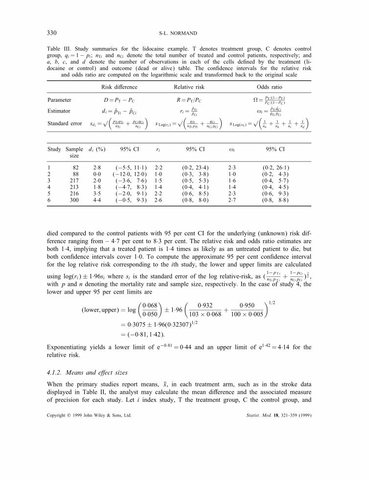
Table III demonstrates three potential study summary statistics for binary measurements usingthe lidocaine data: the di!erence between two probabilities (risk di!erence), the ratio of twoprobabilities (relative risk), and the ratio of the odds for the treated group to the odds for thecontrol group (odds ratio). Risk di!erences are easy to interpret, are de"ned for boundary values(proportions of 0 or 1), and are approximately normally distributed for modest sample sizes.Relative risks and odds ratios are typically analysed on the logarithmic scale, but, unlike the riskdi!erence, are not de"ned for boundary values.Generally inferences in the lidocaine studies remain the same regardless of the choice of sum-

mary statistic. The direction and signi"cance of the study-speci"c e!ects are essentially the sameregardless of the summary statistic selected. Each 95 per cent con"dence interval for the risk dif-ference covers 0 and similarly, the relative risks and odds ratios cover 1. For example, in study 4with a total sample size of 213 patients, an excess of 1·8 per cent of patients treated with lidocaine


330 S-L. NORMAND

Table III. Study summaries for the lidocaine example. T denotes treatment group, C denotes controlgroup, qi =1−pi; nTi and nCi denote the total number of treated and control patients, respectively; anda, b, c, and d denote the number of observations in each of the cells de"ned by the treatment (li-docaine or control) and outcome (dead or alive) table. The con"dence intervals for the relative risk

and odds ratio are computed on the logarithmic scale and transformed back to the original scale

Risk di!erence Relative risk Odds ratio

Parameter D=PT − PC R=PT=PC &= PT=(1−PT)PC=(1−PC)

Estimator di = pTi − pCi ri =pTipCi

!i =pTi qCiqTi pCi

Standard error sdi =√(pTiqTi

nTi+ pCiqCi

nCi

)

s Log(ri) =√( qTi

nTipTi+ qCi

nCipCi

)

s Log(!i) =√( 1

na+ 1

nb+ 1

nc+ 1

nd

)

Study Sample di (%) 95% CI ri 95% CI !i 95% CIsize

1 82 2·8 (−5·5, 11·1) 2·2 (0·2, 23·4) 2·3 (0·2, 26·1)2 88 0·0 (−12·0, 12·0) 1·0 (0·3, 3·8) 1·0 (0·2, 4·3)3 217 2·0 (−3·6, 7·6) 1·5 (0·5, 5·3) 1·6 (0·4, 5·7)4 213 1·8 (−4·7, 8·3) 1·4 (0·4, 4·1) 1·4 (0·4, 4·5)5 216 3·5 (−2·0, 9·1) 2·2 (0·6, 8·5) 2·3 (0·6, 9·3)6 300 4·4 (−0·5, 9·3) 2·6 (0·8, 8·0) 2·7 (0·8, 8·8)

died compared to the control patients with 95 per cent CI for the underlying (unknown) risk dif-ference ranging from – 4·7 per cent to 8·3 per cent. The relative risk and odds ratio estimates areboth 1·4, implying that a treated patient is 1·4 times as likely as an untreated patient to die, butboth con"dence intervals cover 1·0. To compute the approximate 95 per cent con"dence intervalfor the log relative risk corresponding to the ith study, the lower and upper limits are calculated

using log(ri)± 1·96si where si is the standard error of the log relative-risk, as (1−p T inTip T i

+1−pCinCipCi

)12 ,

with p and n denoting the mortality rate and sample size, respectively. In the case of study 4, thelower and upper 95 per cent limits are

(lower; upper) = log(

0·0680·050

)

± 1·96(

0·932103× 0·068 +

0·950100× 0·005

)1=2

= 0·3075± 1·96(0·32307)1=2

= (−0·81; 1·42):

Exponentiating yields a lower limit of e−0·81 = 0·44 and an upper limit of e1·42 = 4·14 for therelative risk.

4.1.2. Means and e!ect sizes

When the primary studies report means, %x, in each treatment arm, such as in the stroke datadisplayed in Table II, the analyst may calculate the mean di!erence and the associated measureof precision for each study. Let i index study, T the treatment group, C the control group, and


META-ANALYSIS 331

nT i and nCi, the respective sample sizes in the two arms. A potential summary measure is thedi!erence in means, Yi= %xT i − %xCi with standard error, si, calculated as

s2i = s2pi

(

1nT i

+1nCi

)

with s2pi=(nT i − 1)s2T i + (nCi − 1)s2Ci

nT i + nCi − 2where s2T i and s

2Ci are the treatment and control group sample variances, respectively, for the

ith study. Figure 2 displays the study means, Yi, and 95 per cent intervals based on si for thestroke study. In Figure 2, study 3 comprised 146 patients, specialist stroke unit care patientsremained in the hospital, on average, 55 days less than patients managed routinely, with 95 percent con"dence intervals for the true di!erence ranging from – 61 days to – 48 days. In the casewhen there is no direct measure common to all the studies, it may be possible to transform thestudy-speci"c summary to a standardized (scale-free) statistic denoted an e!ect size. One commonestimator of e!ect size is the standardized mean di!erence which is calculated as the di!erence ofmeans divided by the variability of the measures. For example, using N(!; "2) to denote normallydistributed with mean ! and variance "2, if

Y Tij ∼ N(!T; "2); j=1; 2; : : : ; nT i

Y Cij ∼ N(!C; "2); j=1; 2; : : : ; nCi

then the standardized mean di!erence is de"ned as

#=!T − !C

":

# represents the gain (or loss) as the fraction of the variability of the measurements. An estimatorof #, denoted Hedges’ g, is de"ned as hi=

%Y Ti − %Y Cisp

. The consequences of dividing by an estimate ofthe standard deviation is to have a unitless summary measure so that in instances when ‘success’is measured in di!erent ways across the studies, the results from the primary studies can betransformed to unitless measures and then pooled. The estimated variance of hi is

(

1nT i

+1nCi

)

+#2

2(nT i + nCi);

where #2is the sample estimate of #2.

4.1.3. Other measures

When the summary data from the primary studies consist of test statistics, then it is sometimespossible to recover the estimated e!ect size if the appropriate pieces of information are alsoreported. For example, if the z-statistic is reported, the estimated standardized mean di!erencemay be calculated as

# = z

√

(

1nTi+1nCi

)

:

If the study summaries are signi"cance levels (p-values) then these may also be combined (Hedgesand Olkin,4 Chapter 3) although this method adds little insight in terms of the size of the e!ect andits direction. The reader is referred to Chapter 2 of Rosenthal5 for a summary of the relationshipbetween e!ect sizes and tests of signi"cance.


332 S-L. NORMAND

4.2. Modelling variation in meta-analysis

There are at least three sources of variation to consider before combining summary statistics acrossstudies. First, sampling error may vary among studies. For example, sample sizes range from 82 to300 in the lidocaine example and from 21 to 311 in the stroke example resulting in study summariesestimated with varying degrees of precision. Second, study-level characteristics may di!er amongthe studies. The stroke studies were conducted at both for-pro"t and not-for-pro"t hospitals andthere may be reason to believe the treatment e!ect is di!erent in these two hospital types.Third, there may exist inter-study variation. The "xed-e!ects model introduced in Section 4.2.1assumes each study is measuring the same underlying parameter and that there is no inter-studyvariation. Conversely, the random-e!ects model (introduced in Section 4.2.2) assumes each studyis associated with a di!erent but related parameter.

4.2.1. Fixed-e!ects model

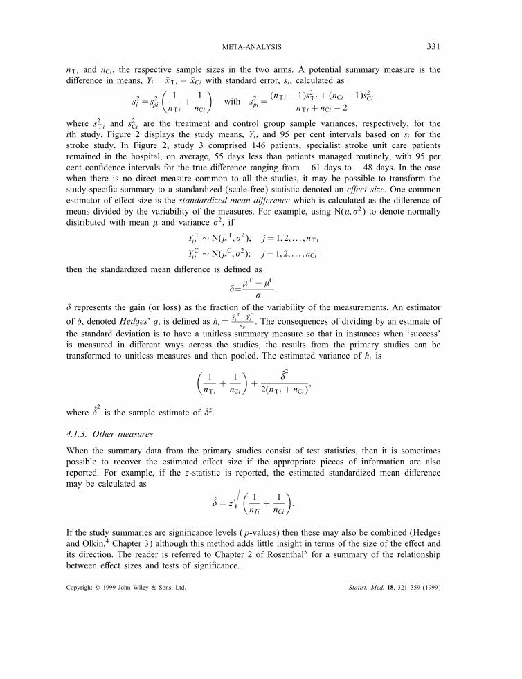
A "xed-e!ects model assumes that each study summary statistic, Yi, is a realization from a popula-tion of study estimates with common mean $ (Figure 3). Let $ be the central parameter of interestand assume there are i=1; 2; : : : ; k independent studies. Assume that Yi is such that E(Yi)= $ andlet s2i =var(Yi) be the variance of the summary statistic in the ith study. For moderately largestudy sizes, each Yi should be asymptotically normally distributed (by the central limit theorem)and approximately unbiased. Thus

Yiindep:∼ N($; s2i ) for i=1; 2; : : : ; k (1)

and s2i assumed known. The central parameter of interest is $ which quanti"es the average treatmente!ect.

4.2.2. Random-e!ects model

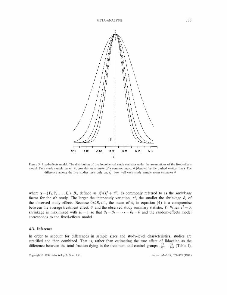
The random-e!ects framework postulates that each study summary statistic, Yi, is a draw from adistribution with a study-speci"c mean, $i, and variance, s2i :

Yi | $i ; s2iindep:∼ N($i ; s2i ): (2)

Furthermore, each study-speci"c mean, $i, is assumed to be a draw from some superpopulation ofe!ects (see discussion in Section 2.1) with mean $ and variance %2 as depicted in Figure 4, with

$i | $; %2indep:∼ N($; %2): (3)

$ and %2 are referred to as hyperparameters and represent, respectively, the average treatmente!ect and inter-study variation.Note that, given the hyperparameters, the distribution of each study summary measure, Yi, after

averaging over the study-speci"c e!ects, is Normal with mean $ and variance s2i + %2. As inthe "xed-e!ects model, $ is a parameter of central interest; however, the between-study variation,%2, plays an important role and must also be estimated. In addition to the average treatmente!ect, it is also possible to derive estimates of the study-speci"c e!ects, $i, that are useful forinferences regarding identifying particularly e!ective studies. The distribution of $i, conditional onthe observed data and the hyperparameters, denoted the posterior distribution, is

$i | y; $; %2∼N(Bi$+ (1− Bi)Yi; s2i (1− Bi)) (4)


META-ANALYSIS 333

Figure 3. Fixed-e!ects model. The distribution of "ve hypothetical study statistics under the assumptions of the "xed-e!ectsmodel. Each study sample mean, Yi , provides an estimate of a common mean, $ (denoted by the dashed vertical line). The

di!erence among the "ve studies rests only on, s2i , how well each study sample mean estimates $

where y=(Y1; Y2; : : : ; Yk). Bi, de"ned as s2i =(s2i + %2), is commonly referred to as the shrinkagefactor for the ith study. The larger the inter-study variation, %2, the smaller the shrinkage Bi ofthe observed study e!ects. Because 06Bi61, the mean of $i in equation (4) is a compromisebetween the average treatment e!ect, $, and the observed study summary statistic, Yi. When %2 = 0,shrinkage is maximized with Bi=1 so that $1 = $2 = · · · = $k = $ and the random-e!ects modelcorresponds to the "xed-e!ects model.

4.3. Inference

In order to account for di!erences in sample sizes and study-level characteristics, studies arestrati"ed and then combined. That is, rather than estimating the true e!ect of lidocaine as thedi!erence between the total fraction dying in the treatment and control groups, 37

557 −21549 (Table I),


334 S-L. NORMAND

Figure 4. Random-e!ects model. The distribution of "ve hypothetical study statistics under the assumptions of the ran-dom-e!ects model. Each e!ect, $i , is drawn from a superpopulation with mean $ and variance %2 (upper plot). Thestudy-speci"c summary statistics, Yi , are then generated from a distribution with mean determined by $i (denoted by ×in the upper plot) and variance s2i (lower plots). In the example, each of the "ve e!ects generated the "ve study results

(lower plots)

a weighted average of the estimates from each study is taken. Similarly, a weighted average ofthe estimates of the treatment e!ects from each for-pro"t hospital study and a weighted averageof the estimates from the not-for-pro"t hospital studies could be taken in the stroke example.However, the distinction of whether each study (or each set of studies) measures a common pa-rameter remains. Therefore the convention is to "rst perform a test of homogeneity of means.If no signi"cant inter-study variation is found, then a "xed-e!ects approach is adopted; otherwisethe meta-analyst either adopts a random-e!ects approach or identi"es study characteristics thatstrati"es the studies into subsets with homogeneous e!ects. The test of homogeneity is next de-scribed and is followed by a description of inferential modes for a "xed-e!ects and random-e!ectsmodel. Maximum likelihood, restricted maximum likelihood and Bayesian methods are given forboth types of models and summarized at the conclusion of this section.


META-ANALYSIS 335

4.3.1. Test of homogeneity

The "xed-e!ects model (equation (1)) assumes that the k study-speci"c summary statistics sharea common mean $. A statistical test for the homogeneity of study means is equivalent to testing

H0: $= $1 = $2 = · · · = $k against

H1: At least one $i di!erent:

Under H0, for large sample sizes, QW =∑k

i Wi(Yi − $MLE)2∼ &2k−1 where $MLE =∑

WiYi=∑

Wiand Wi=1=s2i . If QW is greater than the 100(1 − ') percentile of the &2k−1 distribution, then thehypothesis of equal means, H0, would be rejected at the 100 per cent level. If H0 is rejected,the meta-analyst may conclude that the study means arose from two or more distinct populationsand proceed by either attempting to identify covariates that stratify studies into the homogeneouspopulations or estimating a random-e!ects model. If H0 cannot be rejected the investigator wouldconclude that the k studies share a common mean, $, and estimate $ using $MLE. Tests of homo-geneity have low power against the alternative var($i)¿0. Note that not rejecting H0 is equivalentto asserting that the amount of between-study variation is small.

4.3.2. Fixed-e!ects model

When s2i is assumed known, the log-likelihood for $, log(L($ | y; s2)) is proportional to∑

i((Yi−$)2s2i

) leading to the maximum likelihood estimator (MLE):

$MLE =∑k

i=1WiYi∑k

i=1Wiwith Wi=

1s2i

(5)

where s=(s21 ; s22 ; : : : ; s

2k ). Standard inferences about $ are available using the fact that $MLE∼N($;

(∑

i Wi)−1). A Bayesian approach may be adopted by specifying a prior distribution for $, for

example, $∼N(0; "20 ), and calculating the posterior distribution

$ | y; s; "20 ∼N

⎛

⎝

[

∑

i

Wi + "−20

]−1(∑

i

WiYi

)

;

[

∑

i

Wi + "−20

]−1⎞

⎠ :

The estimator of $ is the posterior mean

$B =

[

∑

i

Wi + "−20

]−1(∑

i

WiYi

)

: (6)

If "20 is large, then the posterior mean coincides with the maximum likelihood estimator.

4.3.3. Random-e!ects model

If %2 is known then the MLE of $ is given by

$(%)MLE =∑

i Wi(%)Yi∑

k Wi(%)with Wi(%)=

1s2i + %2

: (7)


336 S-L. NORMAND

However, in the more realistic case of unknown %2, two common methods of inference can beemployed: restricted maximum likelihood (REML) or Bayesian.

Restricted Maximum Likelihood (REML) This is a method for estimating variance componentsin a general linear model.11; 12 Using the marginal distribution for y, the log-likelihood to bemaximized is

log(L($; %2 | s2; y)∝∑

i

{

log(s2i + %2) +

(Yi − $R)2

s2i + %2

}

+ log(

∑

(s2i + %2)−1

)

:

The REML of %2 is the solution to

%2R =

∑

i w2i (%)

(

kk−1 (Yi − $R)

2 − s2i)

∑

i w2i (%)

:

The estimator for the population mean is then calculated as

$R =∑k

i wi(%R)Yi∑k

i wi(%R); wi(%R)=

1s2i + %2R

(8)

and inferences are made using $R ∼N($; (∑

i wi(%R))−1). An estimator for $i can be calculated by

substituting the REML estimates for the hyperparameters in equation (4). This type of approxima-tion to the posterior distribution is known as empirical Bayes and results in $Ri =(1−BRi )Yi+BRi $Rwhere BRi =

s2i

s2i +%2Ris the shrinkage estimate. Inferences for the study-speci"c e!ects are made using

$Ri ∼N($i ; s2i (1− BRi )): Models can be estimated using the SAS procedure Proc Mixed (see Section5). Note that the empirical Bayes approximation is de"cient in that it ignores the uncertainty inthe hyperparameters, {$; %2}.

Fully Bayesian In order to re#ect the uncertainty in the estimates of hyperparameters $ and %2(equation (3)), a fully Bayesian approach can be adopted.13–16 Prior distributions on the unknownparameters are speci"ed and inferences about the population e!ect $ (and the $is) can be made byintegrating out the unknown parameters over the joint posterior distribution of all the parameters.Let $∼N(0; a2) and %−2∼ gamma(c; d) with E(%−2)= c=d and var(%−2)= c=d2. Then the jointposterior distribution for V =

{

$; $1; : : : ; $k ; %2}

is calculated as:

p(V | y; s2)∝∏

i

p($i |yi; s2i )p($i | $; %2)p($)p(%2):

Inferences are conducted using summaries of the posterior distribution, for example

$B =E($ | y; s2)=∫

$$∫

$i ; %2{p(V ) d$i d%2} d$: (9)

The integral in equation (9) may be analytically tractable when the prior and likelihood are con-jugate. Typically, though, the integral must be evaluated numerically. In cases such as these,Monte Carlo approximations to the posterior, such as those employed in BUGS (see Section 5),may be utilized. Other approximations to the posterior distributions are also available. For ex-ample, Morris17 and Morris and Normand14 proposed an approximation to mean of the posterior


META-ANALYSIS 337

distribution for %2, denoted the adjusted likelihood estimator derived as a result of applying aPearson approximation to the posterior density for %2.

Method of Moments (MOM) A third estimator of %2 is provided by the homogeneity test.By equating QW with its corresponding expected value, DerSimonian and Laird18 proposed anon-iterative (method of moments) estimator of %2 de"ned as

%2DL = max

⎧

⎪

⎪

⎨

⎪

⎪

⎩

0;QW − (k − 1)∑

Wi −∑

W 2i

∑

Wi

⎫

⎪

⎪

⎬

⎪

⎪

⎭

:

This leads to

$DL =∑

i wi(%DL)Yi∑

i wi(%DL)with wi(%DL)=

1s2i + %2DL

: (10)

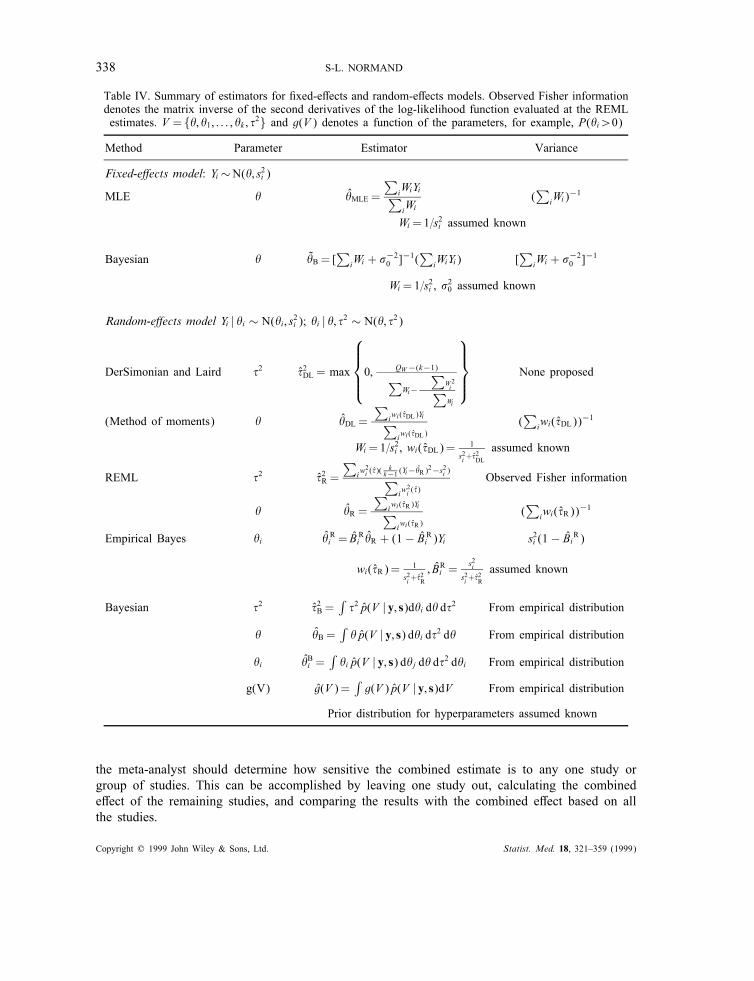
$DL is also denoted Cochran’s semi-weighted estimator of $ and can be easily programmed usingmost software packages. Table IV contains a summary of the estimators that we presented above.

4.4. Diagnostics

Once the data have been collected and analyzed the meta-analyst needs to assess the appro-priateness of the assumptions that have been made. Two aspects of diagnostics are discussed.A systematic approach to investigating how sensitive the results are to the method of analysis orto changes in the data, denoted a sensitivity analysis, is next introduced. Methods for assessingand adjusting the meta-analysis when there is a biased sampling mechanism are also presented.Note that prior to the analysis of the set of primary studies, several quantitative summaries will

have already been collected. The success of the literature retrieval as measured by the recall andprecision or as estimated using capture-recapture models give an indication as to the representa-tiveness of the collected literature (Section 2.3). If a panel of raters has been used to determine theappropriateness of the studies, then inter- and intra-rater reliability statistics are useful measuresof quality; similarly, inter- and intra-coder reliability statistics provide guidance as to the accuracyof the data underlying the meta-analysis.

4.4.1. Sensitivity analysis

An exploratory analysis of the primary data, for example, the study-speci"c estimates, should "rstbe undertaken in order to understand important features of the data. For example, a box plot of thestudy e!ects will indicate typical values, spread (skewness, multi-modal etc.), and tails (presenceof outliers). The box plots may be strati"ed by characteristics of the studies (including qualityscores if available) in order to understand how and why studies di!er. However, if the numberof studies is small, as in the two examples in this article, then the meta-analyst is limited to therange of descriptive analyses that can be undertaken.The meta-analyst should estimate both a "xed-e!ects and a random-e!ects model and compare

the results of both. Sensitivity to the distributional assumptions can be assessed by assumingdi!erent distributions for the study e!ects and comparing subsequent inferences. For example, theanalyst may assume that the underlying study e!ects, $i, arise from a Student-t distribution, therebypermitting heavier tails than those arising from a Normal distribution. Moreover, within a model,


338 S-L. NORMAND

Table IV. Summary of estimators for "xed-e!ects and random-e!ects models. Observed Fisher informationdenotes the matrix inverse of the second derivatives of the log-likelihood function evaluated at the REMLestimates. V = {$; $1; : : : ; $k ; %2} and g(V ) denotes a function of the parameters, for example, P($i¿0)

Method Parameter Estimator Variance

Fixed-e!ects model: Yi ∼N($; s2i )

MLE $ $MLE =

∑

iWiYi∑

iWi(∑

iWi)−1

Wi =1=s2i assumed known

Bayesian $ $B = [∑

iWi + "−20 ]

−1(∑

iWiYi) [∑

iWi + "−20 ]

−1

Wi =1=s2i , "20 assumed known

Random-e!ects model Yi | $i ∼ N($i ; s2i ); $i | $; %2 ∼ N($; %2)

DerSimonian and Laird %2 %2DL = max

⎧

⎪

⎪

⎨

⎪

⎪

⎩

0; QW−(k−1)∑

Wi−

∑

W2i∑

Wi

⎫

⎪

⎪

⎬

⎪

⎪

⎭

None proposed

(Method of moments) $ $DL =∑

iwi(%DL)Yi∑

iwi(%DL)(∑

iwi(%DL))−1

Wi =1=s2i , wi(%DL)= 1s2i +%

2DL

assumed known

REML %2 %2R =∑

iw2i (%)(

kk−1 (Yi−$R)

2−s2i )∑

iw2i (%)

Observed Fisher information

$ $R =∑

iwi(%R)Yi∑

iwi(%R)(∑

iwi(%R))−1

Empirical Bayes $i $ Ri = B Ri $R + (1− B Ri )Yi s2i (1− BiR)

wi(%R)= 1s2i +%

2R

; BRi =s2i

s2i +%2R

assumed known

Bayesian %2 %2B =∫

%2p(V | y; s)d$i d$ d%2 From empirical distribution

$ $B =∫

$p(V | y; s) d$i d%2 d$ From empirical distribution

$i $Bi =∫

$ip(V | y; s) d$j d$ d%2 d$i From empirical distribution

g(V) g(V )=∫

g(V )p(V | y; s)dV From empirical distribution

Prior distribution for hyperparameters assumed known

the meta-analyst should determine how sensitive the combined estimate is to any one study orgroup of studies. This can be accomplished by leaving one study out, calculating the combinede!ect of the remaining studies, and comparing the results with the combined e!ect based on allthe studies.


META-ANALYSIS 339

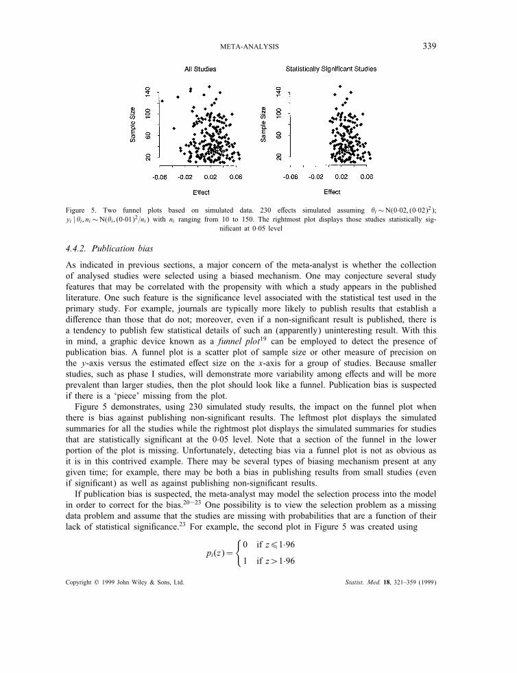
Figure 5. Two funnel plots based on simulated data. 230 e!ects simulated assuming $i ∼N(0·02; (0·02)2);yi | $i ; ni ∼N($i ; (0·01)2=ni) with ni ranging from 10 to 150. The rightmost plot displays those studies statistically sig-

ni"cant at 0·05 level

4.4.2. Publication bias

As indicated in previous sections, a major concern of the meta-analyst is whether the collectionof analysed studies were selected using a biased mechanism. One may conjecture several studyfeatures that may be correlated with the propensity with which a study appears in the publishedliterature. One such feature is the signi"cance level associated with the statistical test used in theprimary study. For example, journals are typically more likely to publish results that establish adi!erence than those that do not; moreover, even if a non-signi"cant result is published, there isa tendency to publish few statistical details of such an (apparently) uninteresting result. With thisin mind, a graphic device known as a funnel plot19 can be employed to detect the presence ofpublication bias. A funnel plot is a scatter plot of sample size or other measure of precision onthe y-axis versus the estimated e!ect size on the x-axis for a group of studies. Because smallerstudies, such as phase I studies, will demonstrate more variability among e!ects and will be moreprevalent than larger studies, then the plot should look like a funnel. Publication bias is suspectedif there is a ‘piece’ missing from the plot.Figure 5 demonstrates, using 230 simulated study results, the impact on the funnel plot when

there is bias against publishing non-signi"cant results. The leftmost plot displays the simulatedsummaries for all the studies while the rightmost plot displays the simulated summaries for studiesthat are statistically signi"cant at the 0·05 level. Note that a section of the funnel in the lowerportion of the plot is missing. Unfortunately, detecting bias via a funnel plot is not as obvious asit is in this contrived example. There may be several types of biasing mechanism present at anygiven time; for example, there may be both a bias in publishing results from small studies (evenif signi"cant) as well as against publishing non-signi"cant results.If publication bias is suspected, the meta-analyst may model the selection process into the model

in order to correct for the bias.20–23 One possibility is to view the selection problem as a missingdata problem and assume that the studies are missing with probabilities that are a function of theirlack of statistical signi"cance.23 For example, the second plot in Figure 5 was created using

pi(z)=

{

0 if z61·96

1 if z¿1·96


340 S-L. NORMAND

where pi(z) denotes the probability of publication of the ith study which depends on its z-value.These proposed methods can be used to provide a broad indication of whether selection bias ispresent, and if it is, the impact of the bias on estimation.

5. SOFTWARE

Estimation of "xed-e!ects models in the context of a meta-analysis is generally straightforwardand can be coded using standard software packages such as S-plus.24 Moreover, there are severalPC-based packages available to perform such analyses (see for example the review by Normand25).Software for estimating random-e!ects models are generally not as accessible. This is particularlytrue in the case of meta-analysis because the user will typically want to force the package tomake use of the known variances, s2i , in the estimation process. For these reasons, two packagesfor performing inference in a random-e!ects model are next introduced. The "rst package is theStatistical Analysis System (SAS) and provides estimates using restricted maximum likelihoodestimation. The second package is a more recently developed system called BUGS (BayesianInference Using Gibbs Sampling) and performs inference within a fully Bayesian framework. Thislist of software is not exhaustive. For example, DuMouchel26 has developed an S-plus functionto implement a fully Bayesian meta-analysis and is publicly available. Rather, the description thatfollows is meant to acquaint the meta-analyst with the computational tactics (and tricks) utilizedwhen performing inference in the random-e!ects model.

5.1. SAS: Proc Mixed

Version 6·11 of SAS provides a procedure denoted Proc Mixed that "ts mixed linear modelsincluding variance component models. A restatement of the random-e!ects model in terms of avariance components model is given by the following:

Y = !1k + !+e; ! ∼Nk(0; %2Ik)

e ∼ Nk(0; R) where R=diag(s21 ; s22 ; : : : ; s

2k )

where Y is a k-vector of observations from the primary studies, 1k is a k-vector of ones, and Ikis the k × k identity matrix. It follows that the study-speci"c e!ect for study i is $i= !+ #i. Thegeneral model estimated in Proc Mixed is

Y = X( + Z)+ e;

) ∼ N(0; G); e∼N(0; R)

where ( is the "xed e!ect, ) is the random e!ect, and e is the error at the study level. Theprocedure permits many di!erent parameterizations for R and G including "xing G and estimatingthe sampling variance, R, but not vice-versa. Unfortunately, in the meta-analysis problem, theuser typically wants to "x the sampling variance R and estimate G. However, users may still useProc Mixed by reversing the roles of the within-study and between-study speci"cations and thenpost-processing the SAS output.


META-ANALYSIS 341

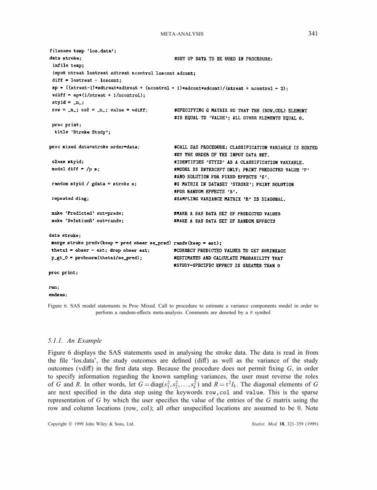
Figure 6. SAS model statements in Proc Mixed. Call to procedure to estimate a variance components model in order toperform a random-e!ects meta-analysis. Comments are denoted by a # symbol

5.1.1. An Example

Figure 6 displays the SAS statements used in analysing the stroke data. The data is read in fromthe "le ‘los.data’, the study outcomes are de"ned (di!) as well as the variance of the studyoutcomes (vdi!) in the "rst data step. Because the procedure does not permit "xing G, in orderto specify information regarding the known sampling variances, the user must reverse the rolesof G and R. In other words, let G=diag(s21 ; s

22 ; : : : ; s

2k ) and R= %

2Ik . The diagonal elements of Gare next speci"ed in the data step using the keywords row,col and value. This is the sparserepresentation of G by which the user speci"es the value of the entries of the G matrix using therow and column locations (row, col); all other unspeci"ed locations are assumed to be 0. Note


342 S-L. NORMAND

that rather than "tting the model

Yi= ! + #i + ei; #i∼N(0; %2); ei∼N(0; s2i ) (11)

the model SAS estimates is

Yi= ! + #∗i + e∗i ; #∗i ∼N(0; si); e∗i ∼N(0; %2): (12)

The data set is printed and next the procedure Proc Mixed is called using the data set strokeand sorted by the order in which they appear in the data set. Class designates which variableswill be used as strati"ers or classi"ers in the subsequent analyses. The model statement indicatesthat the dependent variable is di! and is a function of an intercept term only (note the default isto include an intercept term). The user speci"es the ‘p’ option to print the predicted values, forexample, !+#∗i , and to print an estimate of the overall mean, !, using the ‘s’ option. The randomstatement designates the random-e!ects and does not include an intercept by default. Thus, ‘styid’is speci"ed as a random-e!ect and G is "xed by using the gdata option. This option indicatesthat the G matrix is to read in from the SAS data set ‘stroke’ and using the keywords col, row,and value. The ‘s’ option in the random statement requests that the estimated random-e!ects, #∗ibe printed. The repeated statement is used to specify the R matrix. In the example, R is speci"edusing the keyword ‘diag’ to indicate that R is a diagonal matrix, R= %2Ik . By default, REML isthe estimation method for the covariance parameters.

Post-Processing SAS Output to Get Shrinkage Estimates. Because the roles of G and R havebeen reversed, in order to obtain the correct study-speci"c e!ect estimates, $i, the user needs toprocess the output further. Speci"cally, the shrinkage estimate for the ith study is calculated as

$i= ! + #i=Yi − #∗i :

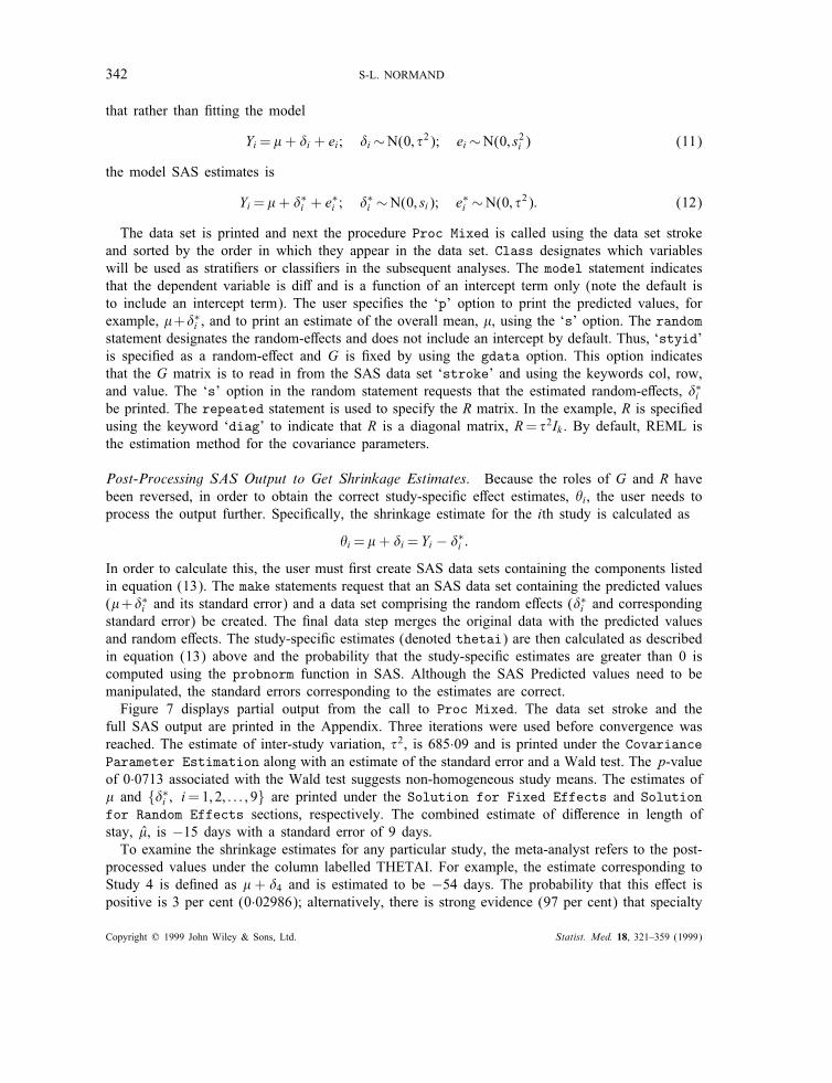
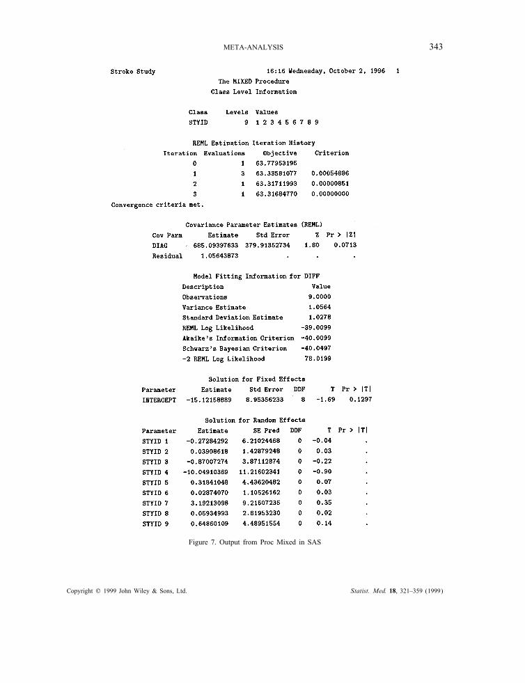
In order to calculate this, the user must "rst create SAS data sets containing the components listedin equation (13). The make statements request that an SAS data set containing the predicted values(!+#∗i and its standard error) and a data set comprising the random e!ects (#∗i and correspondingstandard error) be created. The "nal data step merges the original data with the predicted valuesand random e!ects. The study-speci"c estimates (denoted thetai) are then calculated as describedin equation (13) above and the probability that the study-speci"c estimates are greater than 0 iscomputed using the probnorm function in SAS. Although the SAS Predicted values need to bemanipulated, the standard errors corresponding to the estimates are correct.Figure 7 displays partial output from the call to Proc Mixed. The data set stroke and the

full SAS output are printed in the Appendix. Three iterations were used before convergence wasreached. The estimate of inter-study variation, %2, is 685·09 and is printed under the CovarianceParameter Estimation along with an estimate of the standard error and a Wald test. The p-valueof 0·0713 associated with the Wald test suggests non-homogeneous study means. The estimates of! and {#∗i ; i=1; 2; : : : ; 9} are printed under the Solution for Fixed Effects and Solutionfor Random Effects sections, respectively. The combined estimate of di!erence in length ofstay, !, is −15 days with a standard error of 9 days.To examine the shrinkage estimates for any particular study, the meta-analyst refers to the post-

processed values under the column labelled THETAI. For example, the estimate corresponding toStudy 4 is de"ned as ! + #4 and is estimated to be −54 days. The probability that this e!ect ispositive is 3 per cent (0·02986); alternatively, there is strong evidence (97 per cent) that specialty


META-ANALYSIS 343

Figure 7. Output from Proc Mixed in SAS


344 S-L. NORMAND

Figure 7. Continued

stroke care is associated with shorter length of stay compared to routine management. Examinationof the shrinkage estimate for study 6 indicates that shorter lengths of stays are equally probablewhen managed under routine management or specialty care (P GT 0=0·54).

5.2. BUGS

BUGS (version 0·501) is a software package written in Modula-2 and distributed as compiledcode.27; 28 The software conducts Bayesian inference using a Monte Carlo Markov chain techniquecalled Gibbs sampling. The basic sampling approach employed in BUGS is adaptive rejectionsampling using log-concave distributions. The syntax is surprisingly similar to S-plus so manyusers will feel comfortable using BUGS.


META-ANALYSIS 345

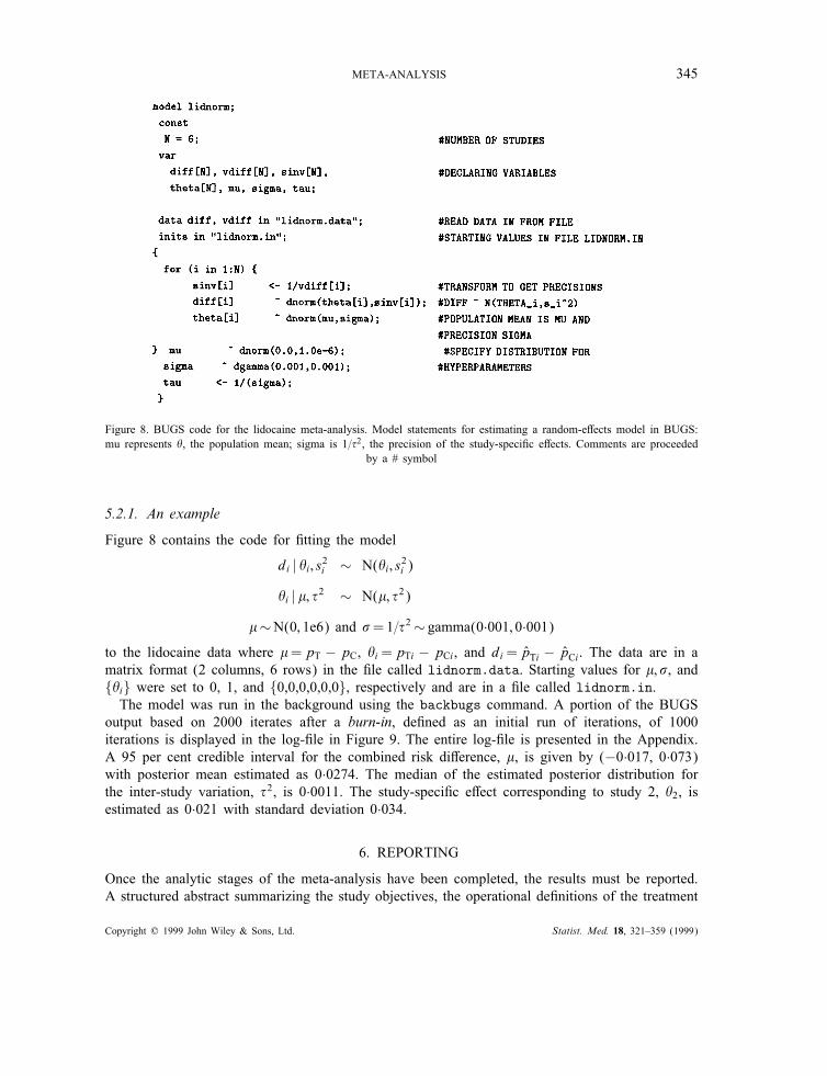
Figure 8. BUGS code for the lidocaine meta-analysis. Model statements for estimating a random-e!ects model in BUGS:mu represents $, the population mean; sigma is 1=%2, the precision of the study-speci"c e!ects. Comments are proceeded

by a # symbol

5.2.1. An example

Figure 8 contains the code for "tting the model

di | $i ; s2i ∼ N($i ; s2i )

$i | !; %2 ∼ N(!; %2)

!∼N(0; 1e6) and "=1=%2∼ gamma(0·001; 0·001)

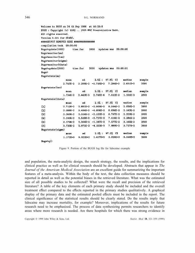
to the lidocaine data where !=pT − pC, $i=pTi − pCi, and di= pTi − pCi. The data are in amatrix format (2 columns, 6 rows) in the "le called lidnorm.data. Starting values for !; ", and{$i} were set to 0, 1, and {0,0,0,0,0,0}, respectively and are in a "le called lidnorm.in.The model was run in the background using the backbugs command. A portion of the BUGS

output based on 2000 iterates after a burn-in, de"ned as an initial run of iterations, of 1000iterations is displayed in the log-"le in Figure 9. The entire log-"le is presented in the Appendix.A 95 per cent credible interval for the combined risk di!erence, !, is given by (−0·017, 0·073)with posterior mean estimated as 0·0274. The median of the estimated posterior distribution forthe inter-study variation, %2, is 0·0011. The study-speci"c e!ect corresponding to study 2, $2, isestimated as 0·021 with standard deviation 0·034.

6. REPORTING

Once the analytic stages of the meta-analysis have been completed, the results must be reported.A structured abstract summarizing the study objectives, the operational de"nitions of the treatment


346 S-L. NORMAND

Figure 9. Portion of the BUGS log "le for lidocaine example

and population, the meta-analytic design, the search strategy, the results, and the implications forclinical practice as well as for clinical research should be developed. Abstracts that appear in TheJournal of the American Medical Association are an excellent guide for summarizing the importantfeatures of a meta-analysis. Within the body of the text, the data collection measures should bereported in detail as well as the potential biases in the retrieved literature. What was the estimatedsize of all possible studies to be collected? What were the recall and precision of the retrievedliterature? A table of the key elements of each primary study should be included and the overalltreatment e!ect compared to the e!ects reported in the primary studies qualitatively. A graphicaldisplay of the primary data and the estimated pooled e!ects must be included in the report. Theclinical signi"cance of the statistical results should be clearly stated. Do the results imply thatlidocaine may increase mortality, for example? Moreover, implications of the results for futureresearch need to be emphasized. The process of data synthesizing permits researchers to identifyareas where more research is needed. Are there hospitals for which there was strong evidence in


META-ANALYSIS 347

decrease length of stay even though the overall estimate covers 0? Finally, the methodologicallimitations should be stated.

7. PROPHYLACTIC LIDOCAINE USE IN HEART ATTACKS

The objective of the meta-analysis is to determine whether there is a detrimental e!ect of lidocaineon mortality for hospitalized patients with a con"rmed heart attack. The primary data include sixstudies and are reported in Table I. To begin, assume that each estimated risk di!erence, di, is

di∼N(pT − pC; s2i ); i=1; 2; : : : ; 6:

7.1. Homogeneity of study means

A test of equality of means yields QW =∑k

i Wi(Yi − %Yw)2∼ &2k−1 = 0·86 and &20·95;5 = 11·07: Thenull hypothesis of homogeneous study means would not be rejected at the 5 per cent level so thatthe analyst may conclude that the di!erences between the studies are so small that any di!erencesare negligible.

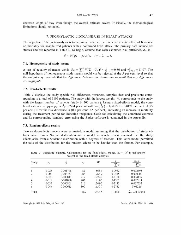
7.2. Fixed-e"ects results

Table V displays the study-speci"c risk di!erences, variances, samples sizes and precisions corre-sponding to a total of 1106 patients. The study with the largest weight, Wi, corresponds to the studywith the largest number of patients (study 6; 300 patients). Using a "xed-e!ects model, the com-bined estimate of pT−pC is %dW =2·94 per cent with var( %dW )= 1=5855·5=0·0171 per cent. A 95per cent CI for the risk di!erence is (0·4 per cent, 5·5 per cent), indicating an increase in mortalityduring the treatment period for lidocaine recipients. Code for calculating the combined estimateand its corresponding standard error using the S-plus software is contained in the Appendix.

7.3. Random-e"ects results

Two random-e!ects models were estimated: a model assuming that the distribution of study ef-fects arise from a Normal distribution and a model in which it was assumed that the studye!ects arise from a Student-t distribution with 4 degrees of freedom. This latter model permittedthe tails of the distribution for the random e!ects to be heavier than the former. For example,

Table V. Lidocaine example. Calculations for the "xed-e!ects model. Wi =1=s2i is the knownweight in the "xed-e!ects analysis

Study di s2di ni Wi Wi∑

Wi

Wi×di∑

Wi

1 0·028 0·001778 82 563·1 0·0962 0·0026952 0·000 0·003757 88 266·2 0·0455 0·0000003 0·020 0·000813 217 1229·7 0·2100 0·0041394 0·018 0·001090 203 917·5 0·1567 0·0028145 0·035 0·000801 216 1248·2 0·2132 0·0075326 0·044 0·000613 300 1630·7 0·2785 0·01226

Total 1106 5855·5 1·0000 %dW =0·02944


348 S-L. NORMAND

E(pTi − pCi |pT − pC; %2; 4)=pT − pC and var(pTi − pCi |pT − pC; %2; 4)=2%2, twice that of aNormal distribution. REML estimates using Proc Mixed were obtained for the model that assumedthe study e!ects are from a Normal distribution; Bayesian estimates using BUGS were obtainedfor both random-e!ects models. In the Bayesian analyses, non-informative proper priors for thepopulation mean and variance were assumed for both random-e!ects models. In particular, pT−pCwas given as N(0·0; 1·0 e6) and %−2∼Gamma(0·001; 0·001). See the article by Smith et al.13 re-garding speci"cation of clinical priors for the population hyperparameters. A burn-in period of1000 iterations were used and inference conducted using the subsequent 2000 iterates.Convergence was achieved after 14 iterations using REML estimation in SAS and resulted in an

estimate of 0 for %2. Because QW is less than the corresponding degrees of freedom, the methodof moments (MOM) estimate of inter-study variation, %2, is also 0. Consequently, the estimates forthe pooled risk di!erence using a "xed-e!ects model, and using the MOM and REML estimatesrandom-e!ects model are identical.The Bayesian estimate of %2 (posterior mean) is the same whether a Student-t distribution or

a Normal distribution is assumed for the study-speci"c risk di!erences. As a rough guide, onemay examine the interval pT − pC ± 1·96% to determine whether the magnitude of %2 is clinicallyimportant. If the distribution of the true risk di!erences is approximately Normal, then one mayexpect 95 per cent of the studies to have true risk di!erences in the range −3·1 per cent to −2·4per cent (using the estimates obtain from the Bayesian-t model). Regardless of the model, thepooled estimate of pT − pC is about 3 per cent. Moreover, even though the Bayesian intervalsfor the pooled estimate include 0, the probability that pT − pC¿0 is 92 per cent. Thus, there isevidence to believe that there is an increase in mortality for lidocaine recipients.

7.4. Diagnostics

The assumption of normality seems reasonable given the observed sample sizes. The combinedestimate of the risk di!erence pooled over the six studies is approximately 3 per cent regardlessof whether a "xed-e!ects model or a random-e!ects model is employed and lies in the range ofobserved primary study summaries. Additionally, the results under the random-e!ects model donot change if we hypothesize that the study-speci"c e!ects arise from a Normal distribution orfrom a Student-t distribution.The pooled estimate appears insensitive to any one study. Each row in Table VI displays

the pooled risk di!erence when dropping the corresponding study under a "xed-e!ects model.For example, the combined estimate of pT − pC when dropping study 1 and assuming %2 = 0 is3 per cent. The results were similar when performing the sensitivity analysis using a random-e!ectsmodel.

7.5. Summary

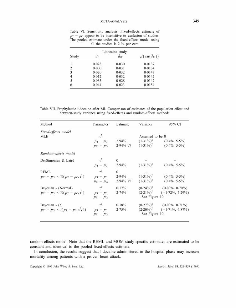
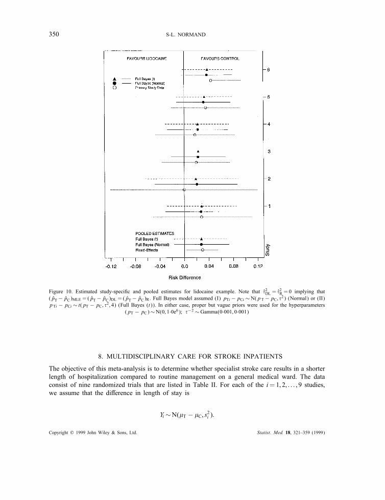
Table VII displays a comparison of the results using "xed-e!ects and random-e!ects models; Figure10 displays the estimated study-speci"c risk di!erences and corresponding 95 per cent con"denceintervals based on the primary study data and credible intervals based on the posterior means.The pooled estimate based on the "xed-e!ects model appears more precise than that based on the

Bayesian model because the former assumes inter-study variation is 0. Conversely, the individualstudy-speci"c estimates using the Bayesian model are associated with more precision than the rawdata because some of the within-study variability is allocated to between-study variability in the


META-ANALYSIS 349

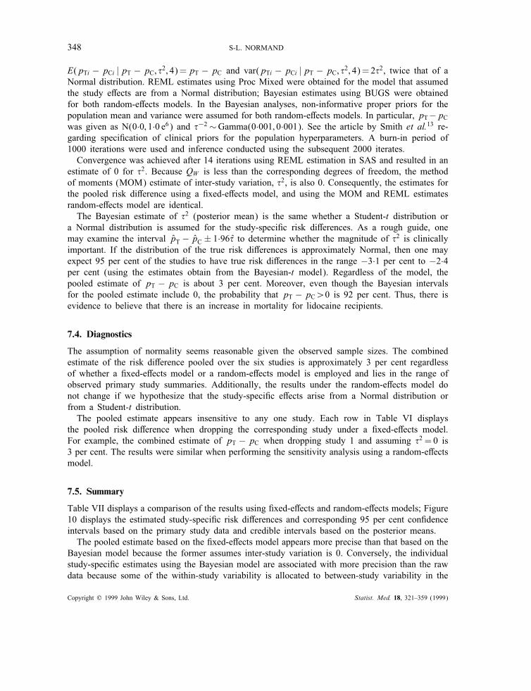
Table VI. Sensitivity analysis. Fixed-e!ects estimate ofpT − pC appear to be insensitive to exclusion of studies.The pooled estimate under the "xed-e!ects model using

all the studies is 2·94 per cent

Lidocaine studyStudy di %dW

√{var( %dW )}

1 0·028 0·030 0·01372 0·000 0·031 0·01343 0·020 0·032 0·01474 0·012 0·032 0·01425 0·035 0·028 0·01476 0·044 0·023 0·0154

Table VII. Prophylactic lidocaine after MI. Comparison of estimates of the population e!ect andbetween-study variance using "xed-e!ects and random-e!ects methods

Method Parameter Estimate Variance 95% CI

Fixed-e!ects modelMLE %2 Assumed to be 0

pT − pC 2·94% (1·31%)2 (0·4%, 5·5%)pTi − pCi 2·94% ∀i (1·31%)2 (0·4%, 5·5%)

Random-e!ects model

DerSimonian & Laird %2 0 – –pT − pC 2·94% (1·31%)2 (0·4%, 5·5%)

REML %2 0 – –pTi − pCi ∼ N(pT − pC; %2) pT − pC 2·94% (1·31%)2 (0·4%, 5·5%)

pTi − pCi 2·94% ∀i (1·31%)2 (0·4%, 5·5%)

Bayesian - (Normal) %2 0·17% (0·24%)2 (0·03%, 0·70%)pTi − pCi ∼ N(pT − pC; %2) pT − pC 2·74% (2·21%)2 (−1·72%, 7·29%)

pTi − pCi See Figure 10

Bayesian - (t) %2 0·18% (0·27%)2 (0·03%, 0·71%)pTi − pCi ∼ t(pT − pC; %2; 4) pT − pC 2·75% (2·20%)2 (−1·71%, 6·87%)

pTi − pCi See Figure 10

random-e!ects model. Note that the REML and MOM study-speci"c estimates are estimated to beconstant and identical to the pooled "xed-e!ects estimate.In conclusion, the results suggest that lidocaine administered in the hospital phase may increase

mortality among patients with a proven heart attack.


350 S-L. NORMAND

Figure 10. Estimated study-speci"c and pooled estimates for lidocaine example. Note that %2DL = %2R = 0 implying that

(pT− pC)MLE = (pT− pC)DL = (pT− pC)R. Full Bayes model assumed (I) pTi−pCi ∼N(p T−pC; %2) (Normal) or (II)pTi − pCi ∼ t(pT − pC; %2; 4) (Full Bayes (t)). In either case, proper but vague priors were used for the hyperparameters

(pT − pC)∼N(0; 1·0e6); %−2∼Gamma(0·001; 0·001)

8. MULTIDISCIPLINARY CARE FOR STROKE INPATIENTS

The objective of this meta-analysis is to determine whether specialist stroke care results in a shorterlength of hospitalization compared to routine management on a general medical ward. The dataconsist of nine randomized trials that are listed in Table II. For each of the i=1; 2; : : : ; 9 studies,we assume that the di!erence in length of stay is

Yi∼N(!T − !C; s2i ):


META-ANALYSIS 351

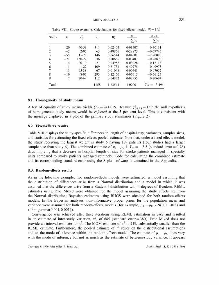
Table VIII. Stroke example. Calculations for "xed-e!ects model. Wi =1=s2i

Study Yi s2Yi ni Wi Wi∑

Wi

Wi×Yi∑

Wi

1 −20 40·59 311 0·02464 0·01507 −0·301312 −2 2·05 63 0·48856 0·29873 −0·597453 −55 15·28 146 0·06544 0·04001 −2·200804 −71 150·22 36 0·00666 0·00407 −0·288905 −4 20·19 21 0·04952 0·03028 −0·121136 1 1·22 109 0·81731 0·49975 0·499757 11 95·38 67 0·01048 0·00641 0·070528 −10 8·03 293 0·12450 0·07613 −0·761279 7 20·69 112 0·04832 0·02955 0·20684

Total 1158 1·63544 1·0000 %YW =−3·494

8.1. Homogeneity of study means

A test of equality of study means yields QW =241·059. Because &20·95;8 = 15·5 the null hypothesisof homogeneous study means would be rejected at the 5 per cent level. This is consistent withthe message displayed in a plot of the primary study summaries (Figure 2).

8.2. Fixed-e"ects results

Table VIII displays the study-speci"c di!erences in length of hospital stay, variances, samples sizes,and statistics for estimating the "xed-e!ects pooled estimate. Note that, under a "xed-e!ects model,the study receiving the largest weight is study 6 having 109 patients (four studies had a largersample size than study 6). The combined estimate of !T−!C is %YW = −3·5 (standard error= 0·78)days implying that a decrease in hospital length of stay for stroke patients managed in specialtyunits compared to stroke patients managed routinely. Code for calculating the combined estimateand its corresponding standard error using the S-plus software is contained in the Appendix.

8.3. Random-e"ects results

As in the lidocaine example, two random-e!ects models were estimated: a model assuming thatthe distribution of di!erences arise from a Normal distribution and a model in which it wasassumed that the di!erences arise from a Student-t distribution with 4 degrees of freedom. REMLestimates using Proc Mixed were obtained for the model assuming the study e!ects are fromthe Normal distribution; Bayesian estimates using BUGS were obtained for both random-e!ectsmodels. In the Bayesian analyses, non-informative proper priors for the population mean andvariance were assumed for both random-e!ects models (for example, !T − !C∼N(0·0; 1·0e6) and%−2∼ gamma(0·001; 0·001)).Convergence was achieved after three iterations using REML estimation in SAS and resulted

in an estimate of inter-study variation, %2, of 685 (standard error= 380). Proc Mixed does notprovide an interval estimate for %2. The MOM estimate of %2 is 219, substantially smaller than theREML estimate. Furthermore, the pooled estimate of %2 relies on the distributional assumptionsand on the mode of inference within the random-e!ects model. The estimate of !T−!C does varywith the mode of inference but not as much as the estimate of between-study variance. It appears


352 S-L. NORMAND

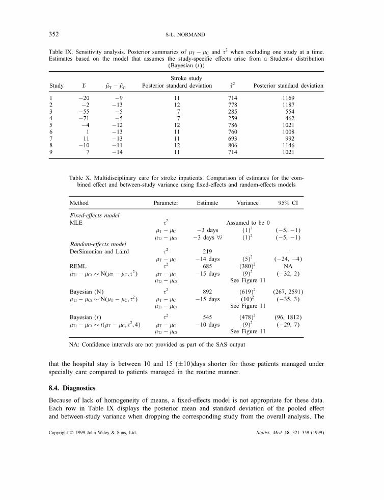
Table IX. Sensitivity analysis. Posterior summaries of !T − !C and %2 when excluding one study at a time.Estimates based on the model that assumes the study-speci"c e!ects arise from a Student-t distribution

(Bayesian (t))

Stroke studyStudy Yi !T − !C Posterior standard deviation %2 Posterior standard deviation

1 −20 −9 11 714 11692 −2 −13 12 778 11873 −55 −5 7 285 5544 −71 −5 7 259 4625 −4 −12 12 786 10216 1 −13 11 760 10087 11 −13 11 693 9928 −10 −11 12 806 11469 7 −14 11 714 1021

Table X. Multidisciplinary care for stroke inpatients. Comparison of estimates for the com-bined e!ect and between-study variance using "xed-e!ects and random-e!ects models

Method Parameter Estimate Variance 95% CI

Fixed-e!ects modelMLE %2 Assumed to be 0

!T − !C −3 days (1)2 (−5, −1)!Ti − !Ci −3 days ∀i (1)2 (−5, −1)

Random-e!ects modelDerSimonian and Laird %2 219 – –

!T − !C −14 days (5)2 (−24, −4)REML %2 685 (380)2 NA!Ti − !Ci ∼ N(!T − !C; %2) !T − !C −15 days (9)2 (−32, 2)

!Ti − !Ci See Figure 11

Bayesian (N) %2 892 (619)2 (267, 2591)!Ti − !Ci ∼ N(!T − !C; %2) !T − !C −15 days (10)2 (−35, 3)


Bayesian (t) %2 545 (478)2 (96, 1812)!Ti − !Ci ∼ t(!T − !C; %2; 4) !T − !C −10 days (9)2 (−29, 7)


NA: Con"dence intervals are not provided as part of the SAS output

that the hospital stay is between 10 and 15 (±10)days shorter for those patients managed underspecialty care compared to patients managed in the routine manner.

8.4. Diagnostics

Because of lack of homogeneity of means, a "xed-e!ects model is not appropriate for these data.Each row in Table IX displays the posterior mean and standard deviation of the pooled e!ectand between-study variance when dropping the corresponding study from the overall analysis. The


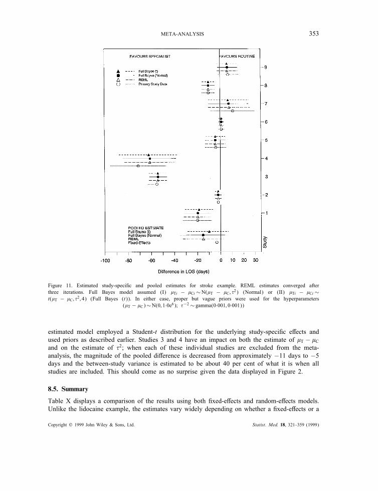
META-ANALYSIS 353

Figure 11. Estimated study-speci"c and pooled estimates for stroke example. REML estimates converged afterthree iterations. Full Bayes model assumed (I) !Ti − !Ci ∼N(!T − !C; %2) (Normal) or (II) !Ti − !Ci ∼t(!T − !C; %2; 4) (Full Bayes (t)). In either case, proper but vague priors were used for the hyperparameters

(!T − !C)∼N(0; 1·0e6); %−2∼ gamma(0·001; 0·001))

estimated model employed a Student-t distribution for the underlying study-speci"c e!ects andused priors as described earlier. Studies 3 and 4 have an impact on both the estimate of !T − !Cand on the estimate of %2; when each of these individual studies are excluded from the meta-analysis, the magnitude of the pooled di!erence is decreased from approximately −11 days to −5days and the between-study variance is estimated to be about 40 per cent of what it is when allstudies are included. This should come as no surprise given the data displayed in Figure 2.

8.5. Summary

Table X displays a comparison of the results using both "xed-e!ects and random-e!ects models.Unlike the lidocaine example, the estimates vary widely depending on whether a "xed-e!ects or a


354 S-L. NORMAND

random-e!ects model is assumed. However, it is clear that a "xed-e!ects model is not supportedby the data.Figure 11 displays the estimated study-speci"c di!erences in length of stay and corresponding

95 per cent con"dence intervals based on the primary study data and credible intervals based onthe posterior means. Because the estimate of %2 is large compared to the within-study variances,there is little shrinkage of the posterior means to the prior mean (for example, Bi=0) so that therandom-e!ects estimates of !Ti − !Ci and corresponding credible intervals are almost identical tothose inferred by using the primary study data alone.In conclusion, specialty stroke care generally resulted in shorter lengths of stay compared to

routine care. Further investigation is needed to determine which aspects of the specialty care areassociated with shorter length of stay and which are generalizable.

9. SUMMARY

In this tutorial, methods were described for combining information across related but independentstudies when the primary studies report a single summary statistic such as a mean di!erence.Analytic methods were con"ned to those cases in which normality of the summary statistic holds.There are many situations for which combining multivariate statistical summaries will be theprimary focus. The methods outlined in this article, however, present an introduction to meta-analysis and a general strategy for inference.Although three potential sources of variation (within-study, systematic between-study variation,

and unexplained between-study variation) were identi"ed as important when synthesizing results,the examples in the tutorial focused primarily on within-study and unexplained between-studyvariation. It is important to note that systematic between-study variation, as measured through"xed characteristics of the studies, zi, may exist and can be accounted for in both the "xed-e!ectsand random-e!ects frameworks. In the case of a "xed-e!ects model, this would be interpretedto mean that treatment e$cacy varies in a systematic fashion between studies characterized byzi and studies not characterizied by zi. In the random-e!ects framework, between-study variationwould be modelled by both study characteristics and random variation. This would be interpretedto mean that the e$cacy within studies characterized by zi is more similar than studies withoutzi, and moreover, the e$cacies within studies characterized by zi di!er because of unexplainedbetween-study variation.

APPENDIX

The S-plus code for performing a "xed-e!ects analysis is included below for both examples utilizedin the tutorial. The complete outputs from two estimation procedures for a random-e!ects modelare also included in this Appendix. The "rst corresponds to the SAS Procedure Proc Mixed forthe stroke study and the second to the BUGS simulation for the lidocaine study.

S-Plus code for the !xed-e"ects lidocaine meta-analysis

gg_matrix(scan("../examples/lidocaine.data"),ncol=4,byrow=T)deadtreat_gg[,3]; deadcontrol_gg[,4]ptreat_gg[,3]/gg[,1]; pcontrol_gg[,4]/gg[,2]ntreat_gg[,1]; ncontrol_gg[,2]


META-ANALYSIS 355

###COMPUTE RISK DIFFERENCES############

diff_ptreat - pcontrolvardiff_ptreat*(1-ptreat)/gg[,1] + pcontrol*(1-pcontrol)/gg[,2]cilower_diff-1.96*sqrt(vardiff); ciupper_diff+1.96*sqrt(vardiff)

## WEIGHTED; FIXED EFFECTS COMBINED ESTIMATE###########

dweights_1/vardiffdbarweighted_sum(dweights*diff)/sum(dweights) #combined estimatevardbarweighted_1/sum(dweights) #variance of estimate

print(c(dbarweighted,sqrt(vardbarweighted)))

S-Plus code for the !xed-e"ects stroke meta-analysis

los_matrix(scan("../examples/los.data"),ncol=6,byrow=T)ntreated_los[,1]; meantreated_los[,2]; sdtreated_los[,3]ncontrol_los[,4]; meancontrol_los[,5]; sdcontrol_los[,6]

difflos_meantreated - meancontrolpooleds_((ntreated-1)*sdtreated^2 + (ncontrol-1)*sdcontrol^2)/(ntreated +ncontrol -2)vardifflos_pooleds*(1/ntreated + 1/ncontrol)cilower_difflos - 1$\cdot$96*sqrt(vardifflos); ciupper_difflos+1$\cdot$96*sqrt(vardifflos)

## - WEIGHTED; FIXED EFFECTS COMBINED ESTIMATE###########

losweights_1/vardiffloslosbarweighted_sum(losweights*difflos)/sum(losweights) #combined estimatevarlosbarweighted_1/sum(losweights) #variance of estimate

print(c(losbarweighted,sqrt(varlosbarweighted)))

SAS output for the random-e"ects stroke meta-analysisStroke Study 14:31 Tuesday, April 16, 1996 1

L NO S C L

N S D O O ST T T N S D V S VR R R T C C D D T A

O E E E R O O I I Y R C LB A A A O N N F S F I O O US T T T L T T F P F D W L E

1 155 55 47 156 75 64 -20 3155.55 40.586 1 1 1 40.5862 31 27 7 32 29 4 -2 32.23 2.047 2 2 2 2.0473 75 64 17 71 119 29 -55 557.33 15.281 3 3 3 15.2814 18 66 20 18 137 48 -71 1352.00 150.222 4 4 4 150.2225 8 14 8 13 18 11 -4 100.00 20.192 5 5 5 20.1926 57 19 7 52 18 4 1 33.27 1.224 6 6 6 1.2247 34 52 45 33 41 34 11 1597.18 95.376 7 7 7 95.3768 110 21 16 183 31 27 -10 551.83 8.032 8 8 8 8.0329 60 30 27 52 23 20 7 576.46 20.694 9 9 9 20.694

Stroke Study 14:31 Tuesday, April 16, 1996 2


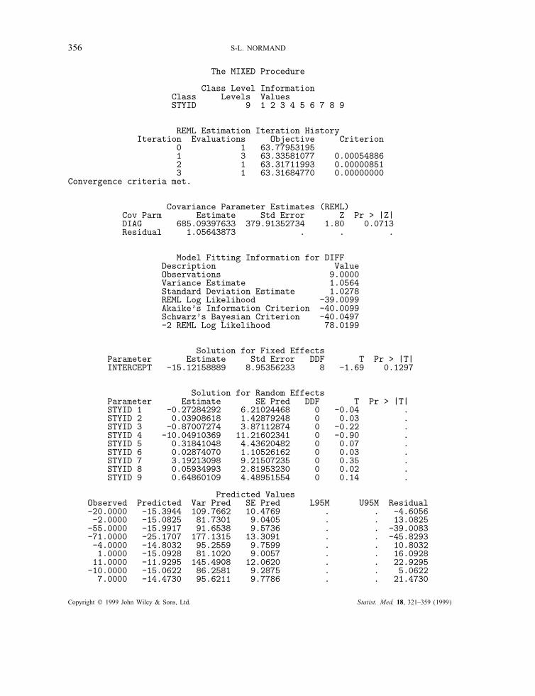
356 S-L. NORMAND

The MIXED Procedure

Class Level InformationClass Levels ValuesSTYID 9 1 2 3 4 5 6 7 8 9

REML Estimation Iteration HistoryIteration Evaluations Objective Criterion

0 1 63.779531951 3 63.33581077 0.000548862 1 63.31711993 0.000008513 1 63.31684770 0.00000000

Convergence criteria met.

Covariance Parameter Estimates (REML)Cov Parm Estimate Std Error Z Pr > |Z|DIAG 685.09397633 379.91352734 1.80 0.0713Residual 1.05643873 . . .

Model Fitting Information for DIFFDescription ValueObservations 9.0000Variance Estimate 1.0564Standard Deviation Estimate 1.0278REML Log Likelihood -39.0099Akaike’s Information Criterion -40.0099Schwarz’s Bayesian Criterion -40.0497-2 REML Log Likelihood 78.0199

Solution for Fixed EffectsParameter Estimate Std Error DDF T Pr > |T|INTERCEPT -15.12158889 8.95356233 8 -1.69 0.1297

Solution for Random EffectsParameter Estimate SE Pred DDF T Pr > |T|STYID 1 -0.27284292 6.21024468 0 -0.04 .STYID 2 0.03908618 1.42879248 0 0.03 .STYID 3 -0.87007274 3.87112874 0 -0.22 .STYID 4 -10.04910369 11.21602341 0 -0.90 .STYID 5 0.31841048 4.43620482 0 0.07 .STYID 6 0.02874070 1.10526162 0 0.03 .STYID 7 3.19213098 9.21507235 0 0.35 .STYID 8 0.05934993 2.81953230 0 0.02 .STYID 9 0.64860109 4.48951554 0 0.14 .

Predicted ValuesObserved Predicted Var Pred SE Pred L95M U95M Residual-20.0000 -15.3944 109.7662 10.4769 . . -4.6056-2.0000 -15.0825 81.7301 9.0405 . . 13.0825

-55.0000 -15.9917 91.6538 9.5736 . . -39.0083-71.0000 -25.1707 177.1315 13.3091 . . -45.8293-4.0000 -14.8032 95.2559 9.7599 . . 10.80321.0000 -15.0928 81.1020 9.0057 . . 16.0928

11.0000 -11.9295 145.4908 12.0620 . . 22.9295-10.0000 -15.0622 86.2581 9.2875 . . 5.0622

7.0000 -14.4730 95.6211 9.7786 . . 21.4730


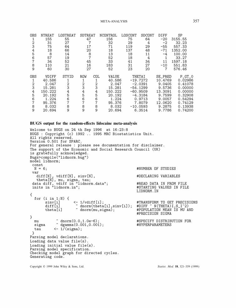
META-ANALYSIS 357

OBS NTREAT LOSTREAT SDTREAT NCONTROL LOSCONT SDCONT DIFF SP1 155 55 47 156 75 64 -20 3155.552 31 27 7 32 29 4 -2 32.233 75 64 17 71 119 29 -55 557.334 18 66 20 18 137 48 -71 1352.005 8 14 8 13 18 11 -4 100.006 57 19 7 52 18 4 1 33.277 34 52 45 33 41 34 11 1597.188 110 21 16 183 31 27 -10 551.839 60 30 27 52 23 20 7 576.46

OBS VDIFF STYID ROW COL VALUE THETAI SE_PRED P_GT_01 40.586 1 1 1 40.586 -19.7272 10.4769 0.029862 2.047 2 2 2 2.047 -2.0391 9.0405 0.410783 15.281 3 3 3 15.281 -54.1299 9.5736 0.000004 150.222 4 4 4 150.222 -60.9509 13.3091 0.000005 20.192 5 5 5 20.192 -4.3184 9.7599 0.329086 1.224 6 6 6 1.224 0.9713 9.0057 0.542947 95.376 7 7 7 95.376 7.8079 12.0620 0.741298 8.032 8 8 8 8.032 -10.0593 9.2875 0.139389 20.694 9 9 9 20.694 6.3514 9.7786 0.74200

BUGS output for the random-e"ects lidocaine meta-analysisWelcome to BUGS on 24 th Sep 1996 at 16:23:8BUGS : Copyright (c) 1992 .. 1995 MRC Biostatistics Unit.All rights reserved.Version 0.501 for SPARC.For general release : please see documentation for disclaimer.The support of the Economic and Social Research Council (UK)is gratefully acknowledged.Bugs>compile("lidnorm.bug")model lidnorm;constN = 6; #NUMBER OF STUDIESvar

diff[N], vdiff[N], sinv[N], #DECLARING VARIABLEStheta[N], mu, sigma, tau;

data diff, vdiff in "lidnorm.data"; #READ DATA IN FROM FILEinits in "lidnorm.in"; #STARTING VALUES IN FILE

LIDNORM.IN{

for (i in 1:N) {sinv[i] <- 1/vdiff[i]; #TRANSFORM TO GET PRECISIONSdiff[i] ~ dnorm(theta[i],sinv[i]); #DIFF ~ N(THETA)I,S_I^2)theta[i] ~ dnorm(mu,sigma); #POPULATION MEAN IS MU AND

#PRECISION SIGMA}

mu ~ dnorm(0.0,1.0e-6); #SPECIFY DISTRIBUTION FORsigma ~ dgamma(0.001,0.001); #HYPERPARAMETERStau <- 1/(sigma);}

Parsing model declarations.Loading data value file(s).Loading initial value file(s).Parsing model specification.Checking model graph for directed cycles.Generating code.


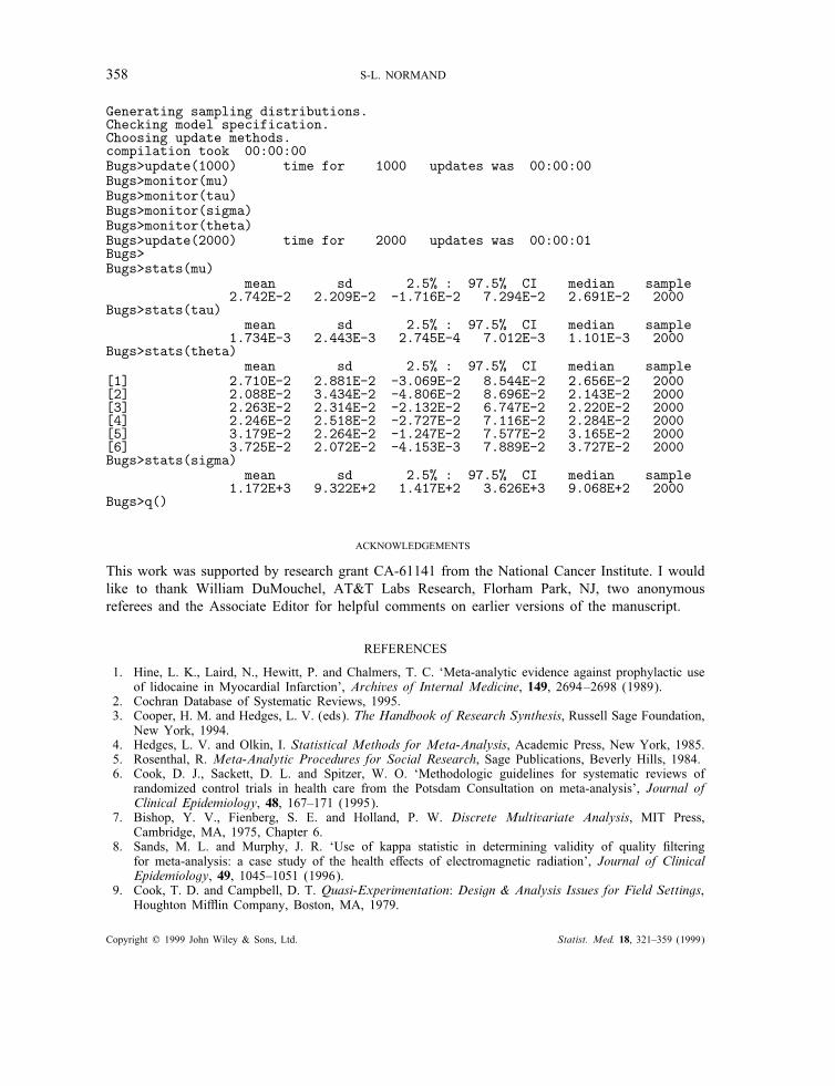
358 S-L. NORMAND

Generating sampling distributions.Checking model specification.Choosing update methods.compilation took 00:00:00Bugs>update(1000) time for 1000 updates was 00:00:00Bugs>monitor(mu)Bugs>monitor(tau)Bugs>monitor(sigma)Bugs>monitor(theta)Bugs>update(2000) time for 2000 updates was 00:00:01Bugs>Bugs>stats(mu)

mean sd 2.5% : 97.5% CI median sample2.742E-2 2.209E-2 -1.716E-2 7.294E-2 2.691E-2 2000

Bugs>stats(tau)mean sd 2.5% : 97.5% CI median sample

1.734E-3 2.443E-3 2.745E-4 7.012E-3 1.101E-3 2000Bugs>stats(theta)

mean sd 2.5% : 97.5% CI median sample[1] 2.710E-2 2.881E-2 -3.069E-2 8.544E-2 2.656E-2 2000[2] 2.088E-2 3.434E-2 -4.806E-2 8.696E-2 2.143E-2 2000[3] 2.263E-2 2.314E-2 -2.132E-2 6.747E-2 2.220E-2 2000[4] 2.246E-2 2.518E-2 -2.727E-2 7.116E-2 2.284E-2 2000[5] 3.179E-2 2.264E-2 -1.247E-2 7.577E-2 3.165E-2 2000[6] 3.725E-2 2.072E-2 -4.153E-3 7.889E-2 3.727E-2 2000Bugs>stats(sigma)

mean sd 2.5% : 97.5% CI median sample1.172E+3 9.322E+2 1.417E+2 3.626E+3 9.068E+2 2000

Bugs>q()

ACKNOWLEDGEMENTS

This work was supported by research grant CA-61141 from the National Cancer Institute. I wouldlike to thank William DuMouchel, AT&T Labs Research, Florham Park, NJ, two anonymousreferees and the Associate Editor for helpful comments on earlier versions of the manuscript.

REFERENCES

1. Hine, L. K., Laird, N., Hewitt, P. and Chalmers, T. C. ‘Meta-analytic evidence against prophylactic useof lidocaine in Myocardial Infarction’, Archives of Internal Medicine, 149, 2694–2698 (1989).

2. Cochran Database of Systematic Reviews, 1995.3. Cooper, H. M. and Hedges, L. V. (eds). The Handbook of Research Synthesis, Russell Sage Foundation,

New York, 1994.4. Hedges, L. V. and Olkin, I. Statistical Methods for Meta-Analysis, Academic Press, New York, 1985.5. Rosenthal, R. Meta-Analytic Procedures for Social Research, Sage Publications, Beverly Hills, 1984.6. Cook, D. J., Sackett, D. L. and Spitzer, W. O. ‘Methodologic guidelines for systematic reviews of

randomized control trials in health care from the Potsdam Consultation on meta-analysis’, Journal ofClinical Epidemiology, 48, 167–171 (1995).

7. Bishop, Y. V., Fienberg, S. E. and Holland, P. W. Discrete Multivariate Analysis, MIT Press,Cambridge, MA, 1975, Chapter 6.

8. Sands, M. L. and Murphy, J. R. ‘Use of kappa statistic in determining validity of quality "lteringfor meta-analysis: a case study of the health e!ects of electromagnetic radiation’, Journal of ClinicalEpidemiology, 49, 1045–1051 (1996).

9. Cook, T. D. and Campbell, D. T. Quasi-Experimentation: Design & Analysis Issues for Field Settings,Houghton Mi'in Company, Boston, MA, 1979.


META-ANALYSIS 359

10. Chalmers, T. C, Smith, H. Jr., Blackburn, B., Silverman, B., Schroeder, B., Reitman, D. and Ambroz, A.‘A method for assessing the quality of a randomized control trial’, Controlled Clinical Trials, 2, 31–49(1981).

11. Patterson, H. D. and Thompson, R. ‘Recovery of interblock information when block sizes are unequal’,Biometrika, 58, 545–554 (1971).

12. Laird, N. M. and Ware, J. H. ‘Random-e!ects models for longitudinal data’, Biometrics, 38, 963–974(1982).

13. Smith, T. C., Spiegelhalter, D. J. and Thomas, A. ‘Bayesian approaches to random-e!ects meta-analysis:a comparative study’, Statistics in Medicine, 14, 2685–2699 (1995).

14. Morris, C. N. and Normand, S. L. ‘Hierarchical models for combining information and for meta-analyses’,Bayesian Statistics 4, Oxford University Press, 1992, pp. 321–344 (with Discussion).

15. DuMouchel, W.H. ‘Bayesian meta-analysis’ in Statistical Methodology in the Pharmaceutical Sciences,Marcel Dekker, New York, NY, 1990, pp. 509–529.

16. DuMouchel, W.H. and Harris, J.E. ‘Bayes methods for combining the results of cancer studies in humansand other species’, Journal of the American Statistical Association, 78, 293–315 (1983).

17. Morris, C.N. ‘Approximating posterior distributions and posterior moments’, Bayesian Statistics 3,Oxford University Press, 1988, pp. 327–344 (with Discussion).

18. DerSimonian R. and Laird, N. ‘Meta-Analysis in Clinical Trials’, Controlled Clinical Trials, 7, 177–188(1986).

19. Light, R. J. and Pillemer, D. B. Summing Up: The Science of Reviewing Research, Harvard UniversityPress, Boston, MA, 1984.

20. Iyengar, S. and Greenhouse, J. ‘Selection models and the "le-drawer problem’ with Discussion,Statistical Science, 3, 109–135 (1988).

21. Dear, K. B. and Begg, C. B. ‘An approach for assessing publication bias prior to performing a meta-analysis’, Statistical Science, 7, 237–245 (1992).

22. Hedges, L. V. ‘Modeling publication selection e!ects in meta-analysis’, Statistical Science, 7, 246–255(1992).

23. Givens, G. F., Smith, D. D. and Tweedie, R. L. ‘Estimating and adjusting for publication bias usingdata augmentation in Bayesian meta-analysis’, Technical Report, Department of Statistics, Colorado StateUniversity, 1995.

24. Statistical Sciences, S-PLUS User’s Manual, Version 3.1 Supplement, Statistical Sciences, Inc., Seattle,WA, 1992.

25. Normand, S. L. ‘Meta-analysis software: a comparative review’, American Statistician, 49, 298–309(1995).

26. DuMouchel, W. H. ‘Predictive cross-validation of Bayesian meta-analysis’, in Bayesian Statistics 5,Oxford University Press, 1996, pp. 107–128, (with Discussion).

27. Spiegelhalter, D. J., Thomas, A. and Best, N. G. ‘Computation on bayesian graphical Models’, inBayesian Statistics 5, Oxford University Press, 1996, pp. 407–425 (with Discussion).

28. Normand, S. L. Discussion of ‘Computation on Bayesian Graphical Models’ by Spiegelhalter, D. J.,Thomas, A. and Best, N. G. in Bayesian Statistics 5, Oxford University Press, 1996, pp. 420–421.


Download - TUTORIAL IN BIOSTATISTICS META-ANALYSIS: FORMULATING, EVALUATING ... · META-ANALYSIS: FORMULATING, EVALUATING, COMBINING, AND REPORTING ... a tutorial on meta-analysis intended for

Top Related