
Tutorial Lectures on MCMC II
Sujit Sahu a
Utrecht: August 2000.
You are here because:
� You would like to see more advanced
methodology.
� Maybe some computer illustration.
aIn close association with Gareth Roberts
�

Outline:
� Convergence Study for Better Design
� Graphical Models
� BUGS illustrations.
� Bayesian Model Choice
� Reversible Jump
� Adaptive Methods
�

Rate of Convergence
Let � ��� define a suitable divergence
measure. Rate of convergence is given by:
� � � �� ���������� �where
� ����� � � �"! � # $ % �&� #'� ��� � � � # � �where
� � is the density of �(� �� �)�*# is a non-negative function taking
care of the effect of the starting point.
For example, if % �&� # is the density of
bivariate normal with correlation + then� � +-, .
.

The rate �� is a global measure of convergence
� does not depend on � � �/� , the starting
point
� not only tells how fast it converges
� but also indicates the auto-correlation
present in the MCMC sequence.
� the last point is concerned with the nse
of ergodic averages.
0

Use � to design MCMC.
Recall: � � cor , for bivariate normal
example.
Can we have faster convergence if
correlations are reduced?
Answer: Yes and No !
No, because the correlation structure
matters a great deal in high dimensions.
1

That is why, Roberts and Sahu (1997)
investigate to see the effects of
� blocking
� parameterization
� correlation structure
� updating schemes
on the Gibbs sampler for Gaussian cases.
2

Extrapolation
� Extrapolate results to the non-normal
cases with similar correlation structure.
� Some of this should work because of
asymptotic normality of the posterior
distribution.
� Two further papers Roberts and Sahu
(2000) and Sahu and Roberts (1999)
investigate the issues in detail.
3
We show:
Under a Gaussian setup the rate of
convergence of the EM/ECM algorithm is
the same as the rate of convergence of the
Gibbs sampler.
Implications:
� if a given problem is easy (hard) for the
EM, then it is easy (hard) for the Gibbs
too.
� can use improvement strategy for one
algorithm to hasten convergence in the
other.
4

Extra benefits of first running the EM:
� EM convergence is easy to assess.
� Can use the lessons learned to
implement the Gibbs.
� Can use the last EM iterate as the
starting point in MCMC.
Further, we also prove the intuitive result
that under conditions the Gibbs may
converge faster than the EM algorithm
which does not use the assumed proper
prior distributions.
5

6Example: Sahu and Roberts (1999)
798�: � ; < =�8 < >?8�: !=@8 A �CB ! D ,, #>E8�: A �CB ! D ,� #
This is called NCEN (not centered).
Priors:
� FHG D ,, � I A J �CK ! K #� FHG D ,� � L A J �CK ! K #� Flat prior for ; .
�NM

HCEN (hierarchically centered)
(Gelfand, Sahu and Carlin, 1995)
798�: � OP8 < >?8�: !OP8 A � ; ! D ,, #>?8�: A ��B ! D ,� #
AUXA (Auxiliary, Meng and Van Dyk, 1997)
798�: � ; < I QSR , =�8 < >E8�:=@8 A �CB ! I T � �VU Q � #>E8�: A �CB ! D ,� #
�W�

NCEN AUXA HCEN
ECM Algorithm
Rate 0.832 0.845 0.287
NIT 3431 150 15
CPU 23.32 5.57 0.25
Gibbs SamplerX0.786 0.760 0.526
X= Principal eigenvalue of the lag 1
auto-correlation matrix of
� ; �(� � !YD , �Z� �,!YD , �Z� �� #
�@�
Outline:
� Convergence Study
� Graphical Models
� BUGS illustrations
� Bayesian Model Choice
� Reversible Jump
� Adaptive Methods
�N.

Directed acyclic graphs (DAG)
For example, the DAG- a graph in which all
edges are directed, and there are no
directed loops-
PSfrag replacements
a b
c
d
expresses the natural factorisation of a joint
distribution into factors each giving the joint
distribution of a variable given its parents
% �C[ ! = ! \]! ^ # � % ��[�#_% � = #_% � \a` [ ! = #b% � ^ `c\ #� 0

The role of graphical models
� Graphical modelling provides a
powerful language for specifying and
understanding statistical models.
� Graphs consist of vertices representing
variables, and edges (directed or
otherwise) that express conditional
dependence properties.
� For setting up MCMC, the graphical
structure assists in identifying which
terms need be in a full conditional.
�@1

Markov Property
Variables are conditionally independent of
their non-descendants, given their parents.PSfrag replacements
a b
c
d
e
f
In the graph shown, c is conditionally
independent of (f, e) given (a, b, d).
Find other conditional independence
relationships yourself.
�N2

Since
% ��� d ` � T de# f % ��� #as a function of � d ,
% �&� # �d hg % ij� d ` � pa � d �lk
!
where � all possible vertices, implies
% ��� d ` � T d # � % i � d ` � pa � d � k mn o d pa � n � % i � n ` � pa � n � k
pa=parents, $ p � everything but p in .
That is, one term for the variable itself, and
one for each of its children.
� 3
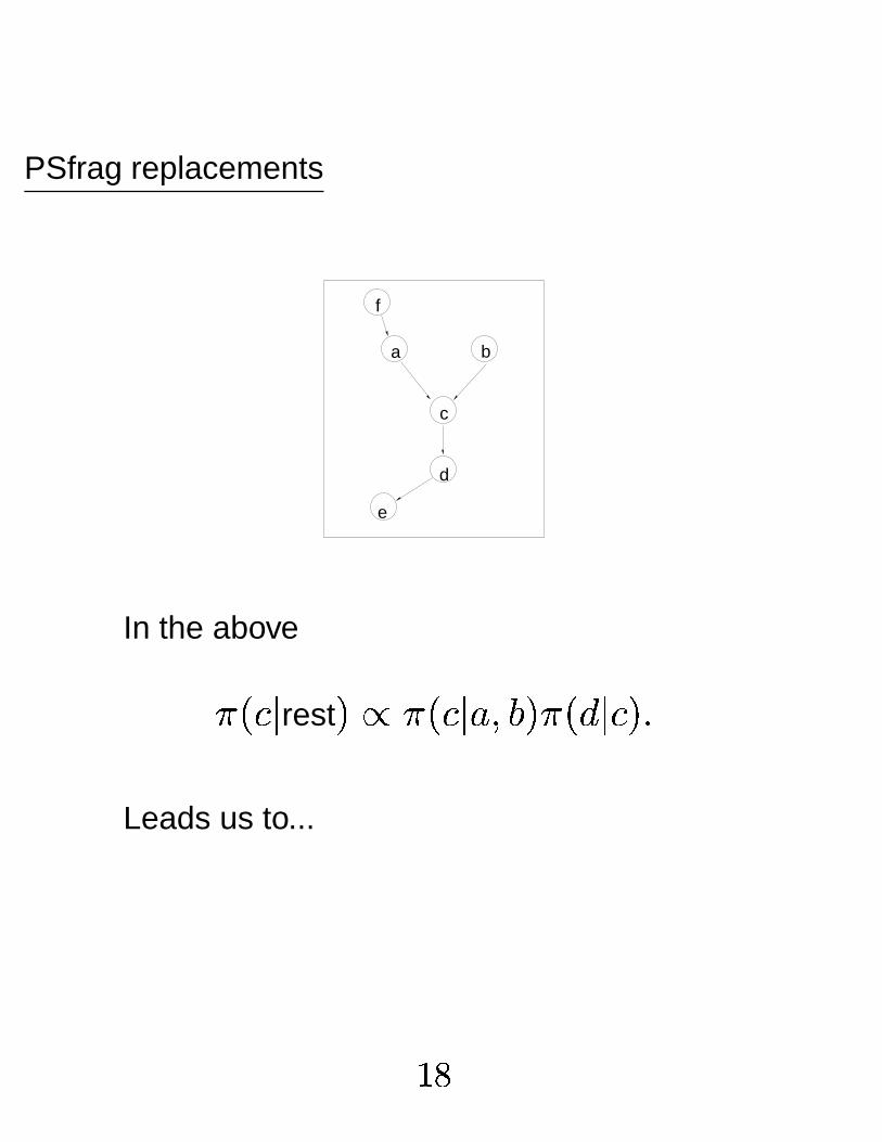
PSfrag replacements
a b
c
d
e
f
In the above
% � \a` rest # f % � \a` [ ! = #b% � ^ `c\ #@qLeads us to...
�N4

Outline:
� Theoretical Convergence Study
� Graphical Models
� BUGS illustrations
� Bayesian Model Choice
� Reversible Jump
� Adaptive Methods
�N5

BUGS
Bayesian inference Using Gibbs Sampling
is a general purpose computer software for
doing MCMC.
� It exploits the structure of the graphical
models to setup the Gibbs sampler.
� It is (still!) freely available from
� www.mrc-bsu.cam.ac.uk
We will go through two non-trivial examples.
(Sorry, no introduction to BUGS).
�rM
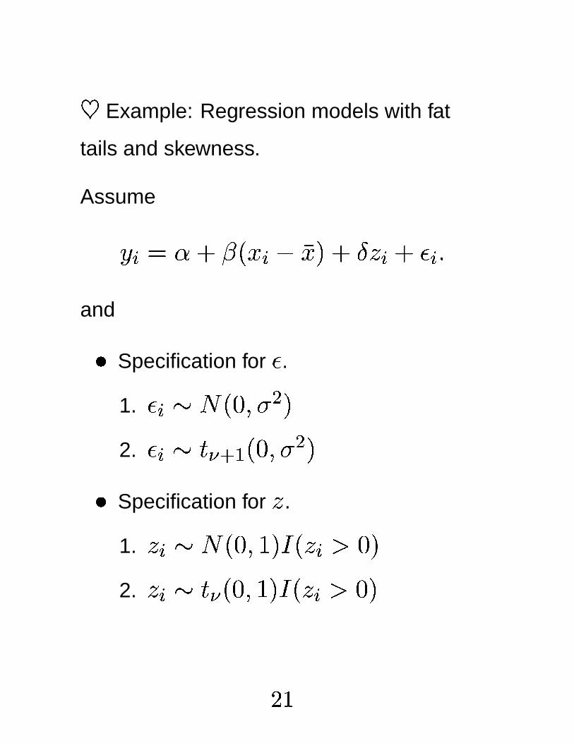
6Example: Regression models with fat
tails and skewness.
Assume
7 8 � s < t �&� 8 $ u� # < Lwv 8 < > 8 qand
� Specification for > .1. >?8 A ��B !YD ,x#2. >?8 A y{z U � ��B ! D ,|#
� Specification for v .
1. v 8 A �CB ! F #b} � v 8 ~ Ba#2. vW8 A y?z ��B ! F #)} � vW8 ~ B�#
�9�

� L , s and t are unrestricted.
� D , and � are given appropriate prior
distributions.
All details including a recent technical
report, computer programs are available
from my home-page.
www.maths.soton.ac.uk/staff/Sahu/utrecht
�W�

Please make your own notes for BUGS in
here.
Basic 5 steps:
� check model
� load data
� compile
� load inits
� gen inits
Then update (from the Model menu) and
Samples (from the Inference menu).
�r.

6Example: A Bayesian test for
determining the number of components in
mixtures.
Develop further the ideas of Mengersen
and Robert (1996).
Let ^ ��� !�� # � ����� � ��� #� �&� # � ��� # ^ �be the Kullback-Leibler distance between �and
�.
Let
� ��� � �&� # � �:@� ��� : � : ��� ` ; : #Sq
We develop an easy to use approximation
for^ ��� ��� � ! � ��� T �V� # .
� 0
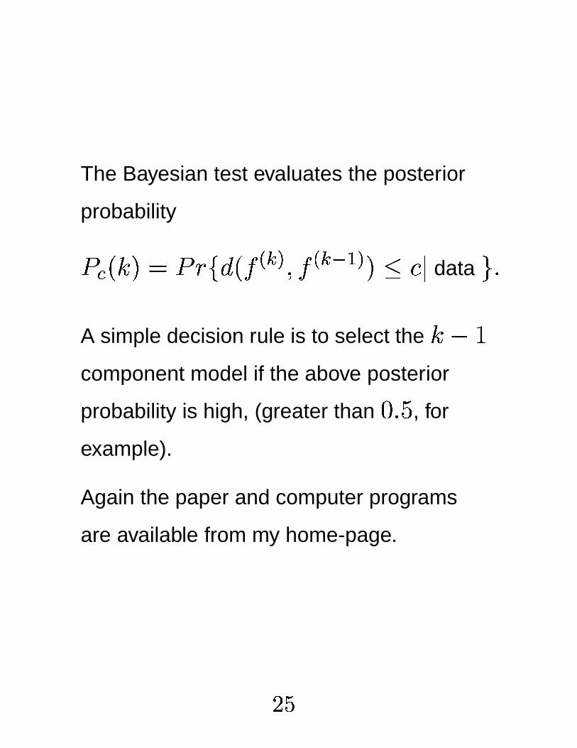
The Bayesian test evaluates the posterior
probability
� ����# � ��� ^ ��� ��� ��! � ��� T �V� # \a`data �-q
A simple decision rule is to select the � $ Fcomponent model if the above posterior
probability is high, (greater than B�q(� , for
example).
Again the paper and computer programs
are available from my home-page.
�W1

Normal Mixtures�
de
nsity
-4 -2 0 2 4�0
.00
.10
.20
.30
.4
PSfrag replacements
Log Bayes factor
Distance
How to choose\?
Height at 0 decreases as distance
increases. Five normal mixtures
corresponding to distance = 0.1, 0.2, 0.3,
0.4 and 0.5.
�r2

Outline:
� Convergence Study
� Graphical Models
� BUGS illustrations.
� Bayesian Model Choice
� Reversible Jump
� Adaptive Methods
� 3
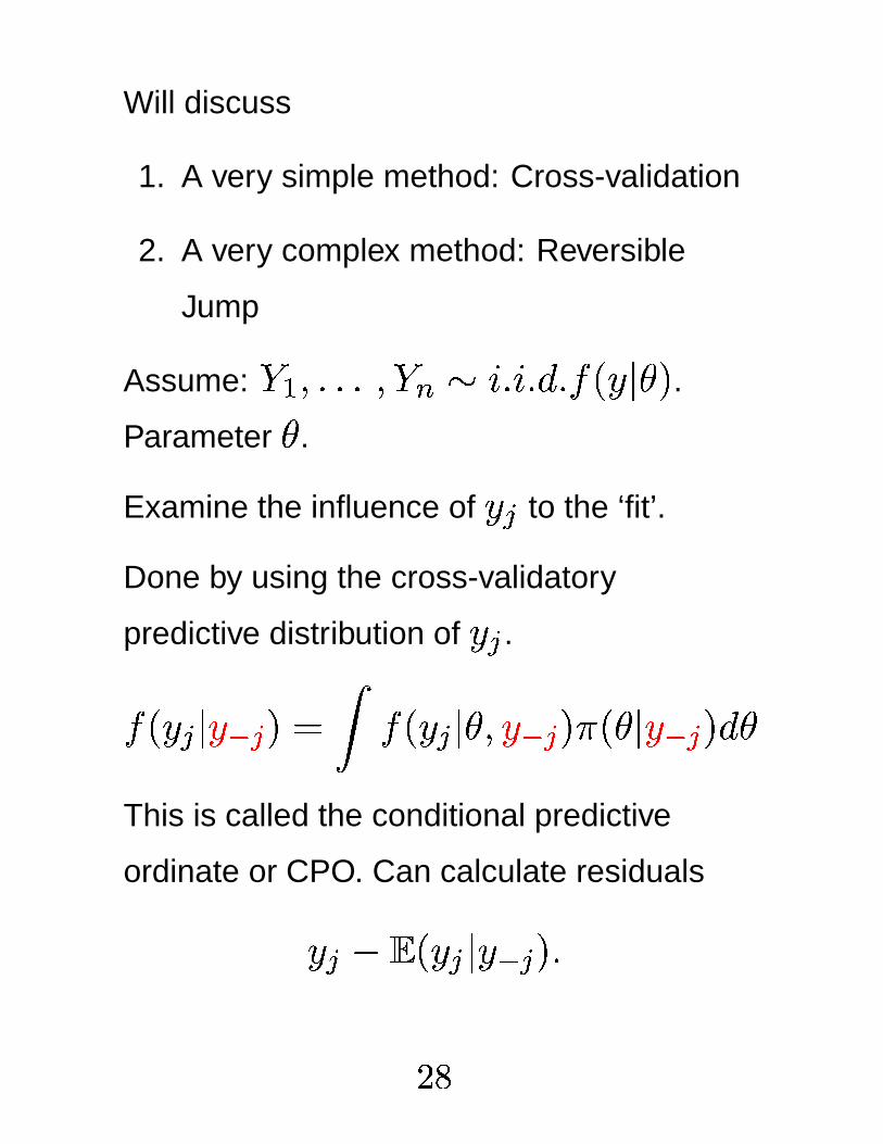
Will discuss
1. A very simple method: Cross-validation
2. A very complex method: Reversible
Jump
Assume: � ! qrqrq ! � A � q � q ^ q�� � 7 ` � # .Parameter
�.
Examine the influence of 7|: to the ‘fit’.
Done by using the cross-validatory
predictive distribution of 7 : .
� � 7|: ` 7 T : # � � � 7|: ` ��! 7 T : #b% � � ` 7 T : # ^¡�This is called the conditional predictive
ordinate or CPO. Can calculate residuals
7W: $ ¢ � 7|: ` 7 T : #Sq�r4
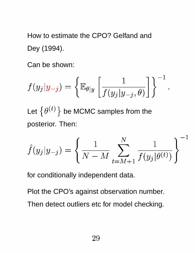
How to estimate the CPO? Gelfand and
Dey (1994).
Can be shown:
� � 7 : ` 7 T : # � ¢ £x¤¦¥ F� � 7 : ` 7 T : !Y� #
T �q
Let� �(� � be MCMC samples from the
posterior. Then:
§� � 7|: ` 7 T : # � F$
¨� � © U �
F� � 7|: ` � �(� � #
T �
for conditionally independent data.
Plot the CPO’s against observation number.
Then detect outliers etc for model checking.
�r5

6Example: Adaptive score data, Cook and
Weisberg (1994).
Simple Linear regression.
•
•
••
•
••
•••
•
•
• •
•••
•
•
•
•
xª
y
10 20 30 40«60
7080
9011
0
••
•• •
• • • • ••
•
• •• • •
•
•
••
Number
cpo
5 10 15 20
-8-7
-6-5
-4
The log(cpo) plot indicates one outliers.
.WM

The psedo-Bayes factor
PsBF � : � � 7 : ` 7 T : ! � #: � � 7|: ` 7 T : ! , #is a variant of the
Bayes factor � Marginal Likelihood under �Marginal Likelihood under , q
There are many other excellent methods
available to calculate the Bayes factor, see
DiCicio et al. (1997) for a review.
We next turn to the second, more complex
method.
.h�

Outline:
� Convergence Study
� Graphical Models
� BUGS illustrations.
� Bayesian Model Choice
� Reversible Jump
� Adaptive Methods
.H�
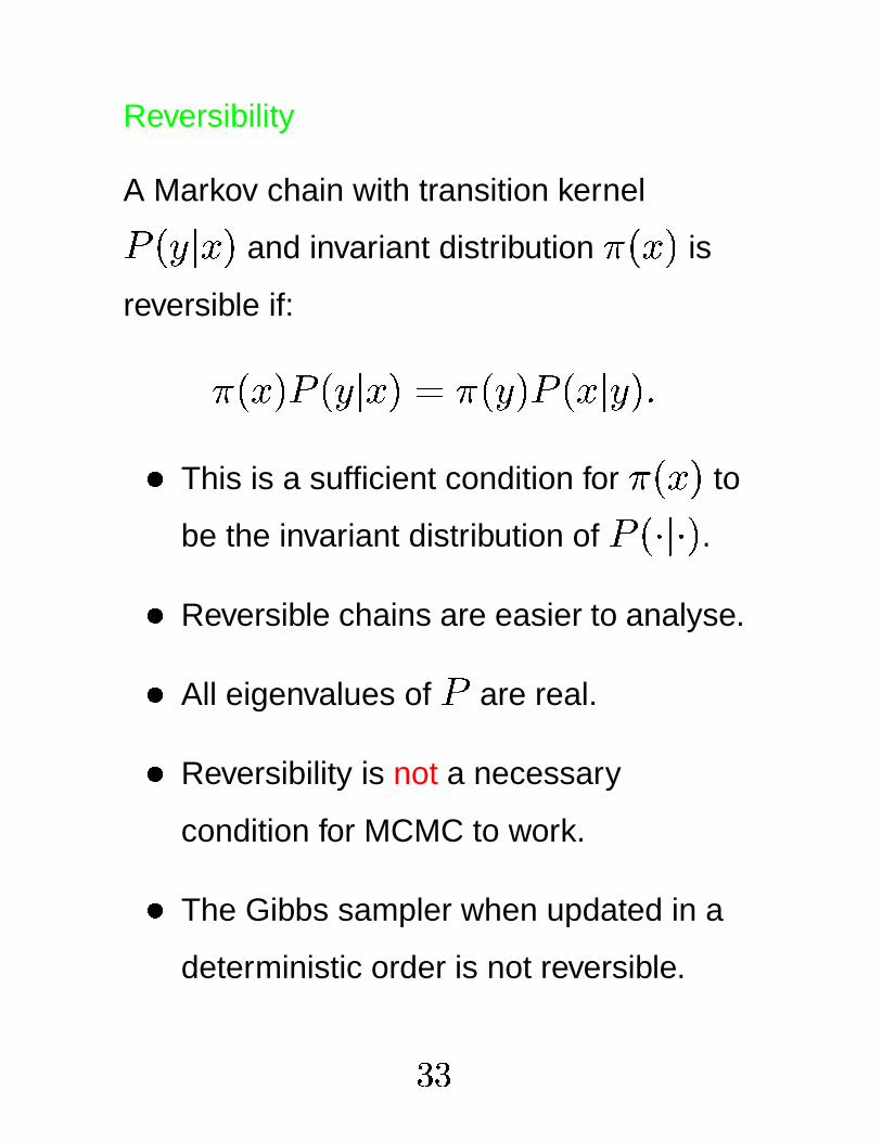
Reversibility
A Markov chain with transition kernel
� 7 ` � # and invariant distribution % �&� # is
reversible if:
% ��� # � 7 ` � # � % � 7 # ��� ` 7 #@q� This is a sufficient condition for % ��� # to
be the invariant distribution of �)� ` �(# .� Reversible chains are easier to analyse.
� All eigenvalues of are real.
� Reversibility is not a necessary
condition for MCMC to work.
� The Gibbs sampler when updated in a
deterministic order is not reversible.
.W.

Jump
Green (1995) extended the
Metropolis-Hastings algorithm for varying
dimensional state space.
Let � ¬ . Conditional on � , the state
space is assumed to be ® � dimensional.
Recall that the acceptance ratio is:
s ��� ! 7 # � ¯ �° F ! % � 7 #% � � #± � � ` 7 #± � 7 ` � # q
Now require that the numerator and
denominator have densities with respect to
a common dominating measure
(“dimension-balancing”). That is, a
dominating measure for the joint distribution
of the current state (in equilibrium) and next
one.
. 0

We need to find a bijection
��� !"² # ³ � 7 ! p´#where
²and p are random numbers of
appropriate dimensions so that
dim ��� !"² # � dim � 7 ! p�# and � 7 ! p´# � µ ��� !�² #where the transformation is one-to-one.
Now the acceptance probability becomes:
s � ��� !�² # ! � 7 ! p´#Y� �¯ �° F ! % � 7 # � , �&p´#% ��� # � � � ² #
¶¶¶¶· µ ��� !"² #· ��� !"² #
¶¶¶¶ qwhere
� � � ² # and�, ��p�# are the densities of²
and p .
How can we understand this?
.H1

The usual M-H ratio:
s ��� ! 7 # � ¯ �° F ! % � 7 #% � � #± � � ` 7 #± � 7 ` � # q
(1)
Now reversible jump ratio:
s � ��� !�² # ! � 7 ! p´#Y� �¯ �° F ! % � 7 # � , �&p´#% ��� # � � � ² #
¶¶¶¶· µ ��� !"² #· ��� !"² #
¶¶¶¶ q(2)
The ratios in the last expression matches
with those of the first.
� The first ratio in (2) exactly comes from
the first ratio in (1). Look at the
arguments of s in both cases.
.W2
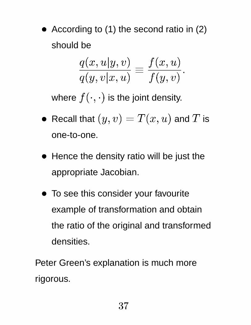
� According to (1) the second ratio in (2)
should be± �&� !"² ` 7 ! p´#± � 7 ! p ` � !�² # ¸ � ��� !�² #� � 7 ! p�# qwhere � �¹� ! �(# is the joint density.
� Recall that � 7 ! p´# � µ ��� !"² # and µ is
one-to-one.
� Hence the density ratio will be just the
appropriate Jacobian.
� To see this consider your favourite
example of transformation and obtain
the ratio of the original and transformed
densities.
Peter Green’s explanation is much more
rigorous.
. 3

ºExample: Enzyme data, Richardson and Green
(1997) Probabilities (after the correction in 1998)
»2 3 4 5 ¼ ½¾ ¿ »�À�ÁH 0.047 0.343 0.307 0.200 0.103
Our distance based approach:
0.0 0.5 1.0 1.5Ã0
24
68
10
PSfrag replacements
Distance
Den
sity
.W4

Outline:
� Convergence Study
� Graphical Models
� BUGS illustrations.
� Bayesian Model Choice
� Reversible Jump
� Adaptive Methods
.W5

Problems with MCMC� Slow convergence...� Problem in estimating nse due to
dependence.
A way forward is to consider Regeneration.
Regeneration points divide the Markov
sample path in i.i.d. tours.
So the tour means can be used as
independent batch means.
Using renewal theory and ratio estimation
can approximate expectations and nse that
are valid without quantifying Markov
dependence.
Mykland, Tierney and Yu (1995), Robert
(1995).
0 M

Regeneration also provides a framework for
adaptation.
Background: Infinite adaptation leads to
bias in the estimates of expectations.
Gelfand and Sahu (1994).
But the bias disappears if adaptation is
performed at regeneration points.
Gilks, Roberts and Sahu (1998) prove a
theorem to this effect and illustrates.
How do you see regeneration points?
0 �

Nummelin’s Splitting.
Suppose that the transition kernel ��� ! K #satisfies
��� ! K # ÄÅ�&� #"� �CK #where � is a probability measure and Ä is a
non-negative function such that
ÄÅ��� #_% � ^ � # ~ B .
Let
� ��� ! � ÆÇ# � ÄÅ��� #E� � ^ � Æ #��� ! ^ � Æ # F !
Now, given a realisation � � � � ! � � �_� ! qrqrqfrom , construct conditionally independent
0/1 random variables È � �/� ! È � �_� ! q|qrq with
0 �

� ��È �(� � � F ` q|qrqN# � � � �Z� � ! � �Z� U �_�From our experience, this is little hard to do
in multi-dimension.
Sahu and Zhigljavsky (1998) provide an
alternative MCMC sampler where
regeneration points are automatically
identified.
Let s ��� # � ��VU É n �(Ê � where
� ��� # � Ë �*Ê �Ì �(Ê � and Í ~ B is a tuning
constant.
0 .

Self Regenerative algorithm:
Let ® � F and Î � B .
� Generate Ï �� � A .
� Generate � � A Geometric � s ��Ï �� � #"# .
If � � ~ B set �ÑÐ U : � � Ï �� �
, forÒ � F ! q|qrq ! � � and Î � Î < � � .
� If ® � then stop, else set
® � ® < F and return to Step I.
Every time � � ~ B is a regeneration point.
0W0
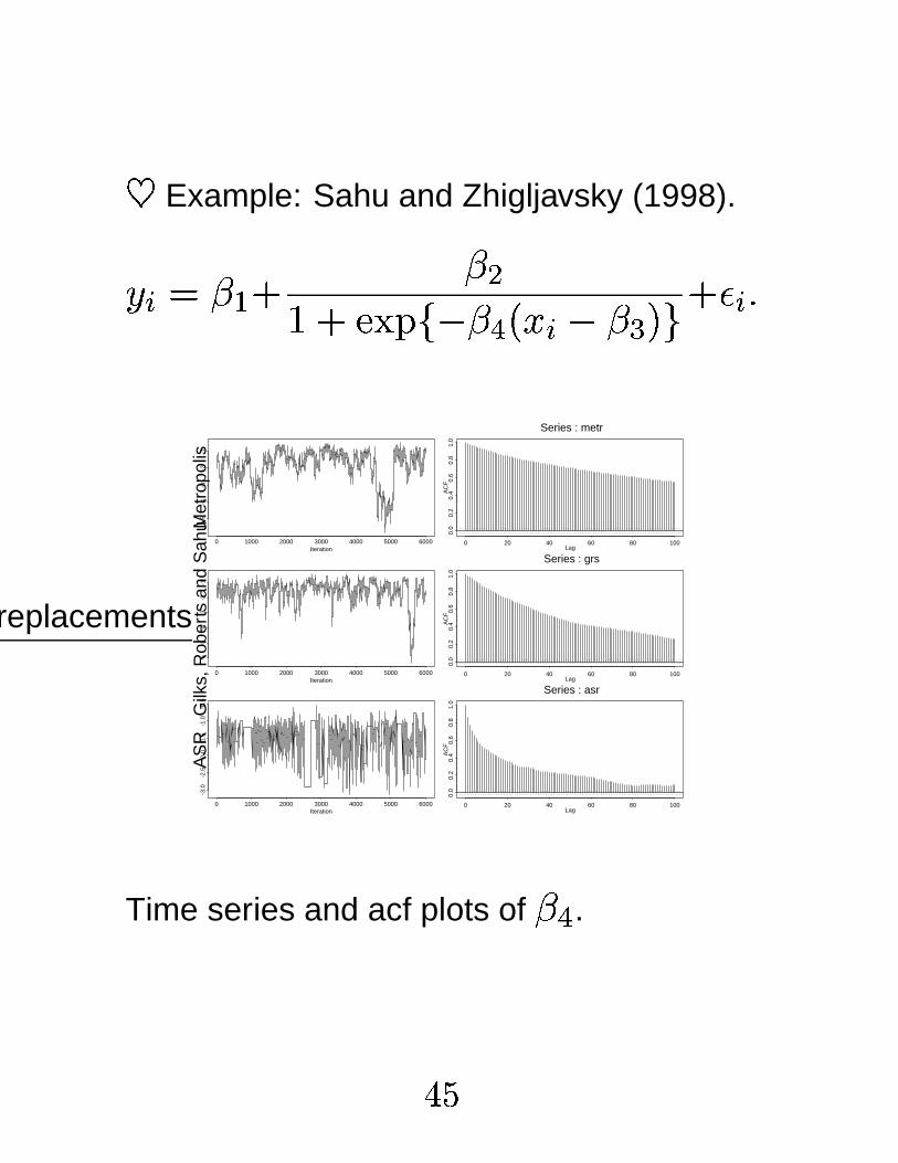
6Example: Sahu and Zhigljavsky (1998).
7 8 � t � < t ,F < ÓÕÔ�Ö � $ t × �&� 8 $ t Ø #Y� < > 8 q
Iteration0 1000 2000 3000 4000 5000 6000
-5-4
-3-2
-1
Lag
AC
F
0 20 40 60 80 100
0.0
0.2
0.4
0.6
0.8
1.0
Series : metr
Iteration0 1000 2000 3000 4000 5000 6000
-6-5
-4-3
-2-1
Lag
AC
F
0 20 40 60 80 100
0.0
0.2
0.4
0.6
0.8
1.0
Series : grs
Iteration0 1000 2000 3000 4000 5000 6000
-3.0
-2.5
-2.0
-1.5
-1.0
-0.5
Lag
AC
F
0 20 40 60 80 100
0.0
0.2
0.4
0.6
0.8
1.0
Series : asr
PSfrag replacements
Met
ropo
lisG
ilks,
Rob
erts
and
Sah
uA
SR
Time series and acf plots of t × .
0 1
Strengths of MCMC
� Freedom in modelling
� Freedom in inference
� Opportunities for simultaneous
inference
� Allows/encourages sensitivity analysis
� Model comparison/criticism/choice
Weaknesses of MCMC
� Order T � R , precision
� Possibility of slow convergence
0 2

Ideas not talked about
Plenty!
� perfect simulation
� particle filtering
� Langevin type methodology
� Hybrid Monte Carlo
� MCMC methods for dynamically
evolving data sets,
Definitely need more fool-proof automatic
methods for large data analysis!
0e3

Online resources
Some links are available from:
www.maths.soton.ac.uk/staff/Sahu/utrecht
� MCMC preprint service (Cambridge)
� Debug: BUGS user group in Germany
� MRC Bio-statistics Unit Cambridge
The Debug site
http://userpage.ukbf.fu-berlin.de/ debug/
maintains a data base of references.
0 4


