
UCGE Reports Number 20333
Department of Geomatics Engineering
Benefits of Combined GPS/GLONASS Processing for High Sensitivity Receivers
(URL: http://www.geomatics.ucalgary.ca/graduatetheses)
by
Mohamed Essam Hassan Roshdy Tamazin
July 2011

UNIVERSITY OF CALGARY
Benefits of Combined GPS/GLONASS Processing for High Sensitivity Receivers
by
Mohamed Essam Hassan Roshdy Tamazin
A THESIS
SUBMITTED TO THE FACULTY OF GRADUATE STUDIES
IN PARTIAL FULFILMENT OF THE REQUIREMENTS FOR THE
DEGREE OF MASTER OF SCIENCE
DEPARTMENT OF GEOMATICS ENGINEERING
CALGARY, ALBERTA
July, 2011
© Mohamed Tamazin 2011

ii
Abstract
This thesis presents a comprehensive study on the advantages of using combined
processing of the Global Positioning System (GPS) and the Global Navigation Satellite
System (GLONASS) for receivers in comparison with a GPS-only receiver in degraded
signal environments. Existing commercial High Sensitivity (HS) GPS receivers suffer
significant degradations in many environments such as in indoor environments and urban
canyons due to restricted visibility of available satellites. Even if a sufficient number of
satellites are available, the geometric Dilution of Precision (DOP), the noise and
multipath can often be large, leading to large errors in position. Currently there are more
than twenty-four active GLONASS satellites in orbit. It is therefore advantageous to
concentrate on combining the GPS and GLONASS measurements to achieve more
reliable and accurate navigation solutions.
In this research, data was collected in an indoor environment and in urban canyons. A
software receiver, namely GSNRx™, was used to process the data in both standard and
high sensitivity modes. The analysis studies the benefits of combined HS
GPS/GLONASS processing in terms of measurement availability, pseudorange
degradation, signal power degradation, navigation solution availability, residual analysis,
positioning accuracy and DOP. The combined use of GLONASS and GPS provides
significant improvement in all of the above performance measures. Recommendations for
future work are made for improvements.

iii
Acknowledgements
My thanks are wholly devoted to ALLAH for His blessings and for helping me to
accomplish this work successfully.
I am honoured that my work has been supervised by Prof. Gérard Lachapelle. I would
like to express my deepest gratitude and sincere appreciation for his help, valuable
advice, continuing support, endless patience and guidance throughout the preparation of
this work. I greatly appreciate his tireless efforts and regular follow-ups while checking
and revising this work, as he was keen on producing an outstanding piece of work.
I wish to express my deep indebtedness and gratitude to my mother and father for their
understanding, encouragement and unconditional support. I also owe special gratitude to
my sister Dina for her help.
I would like to thank Dr. Cillian O’ Driscoll who inspired and motivated me during the
crucial initial stages of my research.
I am thankful to PLAN research engineers, Dr. Jared Bancroft, Dr. Haris Afzal and Dr.
James Curran, for their generosity in sharing knowledge, suggestions and helpful advice.
I also wish to acknowledge a good friend of mine, Dr. Mohamed Youssef, for helping me
right from the time I landed in Calgary. His guidance, technical as well as personal, has
always helped me to take the right steps in my career.
I cannot forget to thank PLAN graduate students, Ahmed Kamel, Billy Chan, Peng Xie,
Pratibha Anantharamu, Shashank Satyanarayana and Tao Lin, for beneficial discussions
and for graciously sharing their time and knowledge with me. Finally, I would like to
thank all my friends in Calgary who continue making my new life here an exciting
experience.

iv
Table of Contents
Abstract .......................................................................................................................... ii Acknowledgements ....................................................................................................... iii Table of Contents ........................................................................................................... iv List of Tables.................................................................................................................vii List of Figures and Illustrations ...................................................................................... ix List of Abbreviations ..................................................................................................... xv
CHAPTER ONE: INTRODUCTION .............................................................................. 1 1.1 Chapter Outline...................................................................................................... 1
1.2 Introduction ........................................................................................................... 1 1.3 Background ........................................................................................................... 2
1.3.1 Urban Canyon and Indoor Positioning ........................................................... 2 1.3.2 Assisted and High Sensitivity GPS Receiver .................................................. 3
1.4 Research Objective ................................................................................................ 4 1.5 Literature Review .................................................................................................. 5
1.6 Thesis Outline ........................................................................................................ 6
CHAPTER TWO: OVERVIEW OF GLONASS .............................................................. 8
2.1 Chapter Outline...................................................................................................... 8 2.2 Overview of GLONASS ........................................................................................ 8
2.2.1 The Space Segment ........................................................................................ 9 2.2.2 The Control Segment ................................................................................... 11
2.2.3 The User Segment........................................................................................ 12 2.2.4 GLONASS Modernization ........................................................................... 12
2.2.4.1 First Generation (GLONASS)............................................................. 13 2.2.4.2 Second Generation (GLONASS-M) .................................................... 13
2.2.4.3 Third Generation (GLONASS-K) ....................................................... 13 2.3 GLONASS Signal Characteristics ........................................................................ 14
2.3.1 GLONASS RF Frequency Plan .................................................................... 15 2.3.2 Signal Structure ........................................................................................... 16
2.3.2.1 Standard Accuracy Ranging Code (C/A-Code) ................................... 17 2.3.2.2 High Accuracy Ranging Code (P-Code) ............................................. 18
2.3.3 Intra-system Interference ............................................................................. 18 2.3.4 GLONASS Navigation Message .................................................................. 19
2.4 Comparison between GPS and GLONASS .......................................................... 19 2.4.1 Time Reference Systems .............................................................................. 20
2.4.1.1 GLONASS Time System .................................................................... 20 2.4.1.2 Time Transformation .......................................................................... 21
2.4.2 Coordinate Systems ..................................................................................... 22 2.4.2.1 PZ-90 (GLONASS) ............................................................................ 22
2.4.2.2 WGS-84 (GPS) ................................................................................... 23 2.5 Advantages of Combined GPS and GLONASS .................................................... 25
CHAPTER THREE: OVERVIEW OF GNSS RECEIVER DESIGN AND TEST MEASURES ......................................................................................................... 27

v
3.1 Chapter Outline.................................................................................................... 27 3.2 General Overview of GNSS Receiver Architecture .............................................. 27
3.2.1 Signal Acquisition ....................................................................................... 32 3.2.2 Signal Tracking............................................................................................ 35
3.3 GNSS Software Receivers – GSNRx™ ................................................................ 36 3.3.1 Overview of GSNRxTM ................................................................................ 37
3.3.2 GSNRxTM Software Receiver Architecture................................................... 37 3.3.3 GSNRx™ Standard versus High Sensitivity Mode ....................................... 40
3.3.4 Assisted High Sensitivity GSNRxTM ............................................................ 41 3.4 Estimation Methods Used .................................................................................... 43
3.4.1 Least-Squares Approach .............................................................................. 44 3.4.2 Kalman Filtering Approach .......................................................................... 48
3.5 Test Measures ...................................................................................................... 52 3.5.1 Measurement Availability ............................................................................ 53
3.5.2 Carrier-to-Noise Density Ratio..................................................................... 53 3.5.3 Fading.......................................................................................................... 53
3.5.4 Position Accuracy, Solution Availability and Dilution of Precision .............. 54
CHAPTER FOUR: STATIC TEST RESULTS AND ANALYSIS ................................. 55
4.1 Chapter Overview ................................................................................................ 55 4.2 Static Tests .......................................................................................................... 55
4.3 Methodology........................................................................................................ 55 4.4 Test Setup and Description .................................................................................. 59
4.5 Experimental Results and Analysis ...................................................................... 61 4.5.1 Wooden House (WH) Test Results ............................................................... 62
4.5.1.1 Measurement Availability ................................................................... 62 4.5.1.2 Carrier-to-Noise Density Ratio ........................................................... 66
4.5.1.3 Fading Analysis .................................................................................. 67 4.5.1.4 Estimated Pseudorange Error .............................................................. 69
4.5.1.5 Position Accuracy, Solution Availability and Dilution of Precision ..... 70 4.5.2 Engineering Laboratory Test Results ........................................................... 78
4.5.2.1 Measurements Availability ................................................................. 79 4.5.2.2 Carrier-to-Noise Density Ratio ........................................................... 82
4.5.2.3 Fading Analysis .................................................................................. 83 4.5.2.4 Estimated Pseudorange Error .............................................................. 85
4.5.2.5 Position Accuracy, Solution Availability and Dilution of Precision ..... 86
CHAPTER FIVE: DYNAMIC TEST RESULTS AND ANALYSIS ............................. 96
5.1 Chapter Overview ................................................................................................ 96 5.2 Dynamic Test....................................................................................................... 96
5.3 Methodology........................................................................................................ 97 5.4 Test Setup and Description .................................................................................. 97
5.5 Experimental Results & Analysis ....................................................................... 100 5.5.1 Measurements Availability ........................................................................ 100
5.5.2 Standard Receiver Processing Results ........................................................ 100 5.5.2.1 Carrier-to-Noise Density Ratio ......................................................... 102
5.5.2.2 Residual Analysis ............................................................................. 104

vi
5.5.2.3 Position Accuracy, Solution Availability and Dilution of Precision ... 111 5.5.3 High Sensitivity Receiver Processing Results............................................. 122
5.5.3.1 Carrier-to-Noise Density Ratio ......................................................... 123 5.5.3.2 Residual Analysis ............................................................................. 125
5.5.3.3 Position Accuracy, Solution Availability and Dilution of Precision ... 129
CHAPTER SIX: CONCLUSIONS AND RECOMMENDATIONS ............................. 138
6.1 Chapter Outline.................................................................................................. 138 6.2 Conclusions ....................................................................................................... 138
6.3 Recommendations .............................................................................................. 140
REFERENCE .............................................................................................................. 141
APPENDIX A LEAST-SQUARES GPS/GLONASS TESTING RESIDUALS WITH ONE DEGREE OF FREEDOM .......................................................................... 145

vii
List of Tables
Table 2-1: GPS/GLONASS Comparison in Space Segment ........................................... 11
Table 2-2: Roadmap of GLONASS Modernization ........................................................ 14
Table 2-3: Elements of PZ-90 System ............................................................................ 23
Table 2-4: Elements of WGS 84 System ........................................................................ 24
Table 2-5: Comparison between GPS and GLONASS ................................................... 25
Table 4-1: Settings Adopted for the Data Collection ...................................................... 61
Table 4-2: WH Test – Satellites Availability Statistics ................................................... 64
Table 4-3: NavLab Test – Satellites Availability Statistics ............................................. 80
Table 5-1: Processing Parameters Used in GSNRx™ ..................................................... 98
Table 5-2: GPS-GLONASS Residuals Statistics - Standard GSNRx™ ........................ 106
Table 5-3: GPS-GLONASS Statistical Representation of Pseudorange Errors Derived from Reference GPS/INS Trajectory - Standard GSNRxTM .................................. 109
Table 5-4: GPS-GLONASS Range Rate Residual Statistics (Downtown, Standard GSNRx™) ........................................................................................................... 111
Table 5-5: Time Series Statistics of Horizontal Position Solutions (Least-Squares, No Height Fixing, Standard GSNRxTM) - Downtown Test ......................................... 116
Table 5-6: Time Series Statistics of Horizontal Position Solutions (Least-Squares, Height Fixing, Standard GSNRxTM) - Downtown Test ......................................... 119
Table 5-7: Time Series Statistics of Horizontal Position Solutions (Kalman Filter, Standard GSNRxTM) - Downtown Test ................................................................ 121
Table 5-8: GPS-GLONASS Pseudorange Statistics (Downtown Test, HS-GSNRx™) . 126
Table 5-9: GPS-GLONASS Statistical Representation of Pseudorange Errors Derived from Reference GPS/INS Trajectory - High Sensitivity GSNRxTM ....................... 128
Table 5-10: GPS-GLONASS Range Rate Residual Statistics - High Sensitivity GSNRxTM ............................................................................................................ 129
Table 5-11: Horizontal Position Solution Statistics (Least Squares, No Height Fixing, HS-GSNRx™) - Downtown Test ......................................................................... 134

viii
Table 5-12: Horizontal Position Solution Statistics (Least Squares, Height Fixing, HS- GSNRx™) - Downtown Test ........................................................................ 136
Table 5-13: Time Series Statistics of Horizontal Position Solutions (Kalman Filter, HS- GSNRx™) - Downtown Test ........................................................................ 137

ix
List of Figures and Illustrations
Figure 2-1: View of the GPS and GLONASS Satellite Orbit Arrangement (NovAtel 2007) ..................................................................................................................... 10
Figure 2-2: GLONASS Antipodal Satellites (Kaplan & Hegarty 2006) .......................... 16
Figure 2-3: L3 CDMA Signal Spectrum (Urlichich et al 2011) ...................................... 17
Figure 2-4: GLONASS C/A-code Generation (GLONASS ICD 2008)........................... 18
Figure 3-1: High Level Architecture of GNSS Receiver (O'Driscoll & Borio 2009) ....... 28
Figure 3-2: Typical RHCP and LHCP Normalized Radiation Pattern of NovAtel Antenna GPS-702 GG for GPS L1 and GLONASS L1 Central Frequency (NovAtel Inc. 2011) ............................................................................................... 28
Figure 3-3: Simplified Block Diagram of a Frequency Mixer......................................... 30
Figure 3-4: Sample Correlation Function ....................................................................... 34
Figure 3-5: A Generic Tracking Loop (Kaplan & Hegarty 2006) ................................... 36
Figure 3-6: General Software Architecture of GSNRx™ (Petovello et al 2008) ............. 38
Figure 3-7: Interaction of Processing Manager and Associated Objects (Petovello et al 2008) ..................................................................................................................... 40
Figure 3-8: Architecture of GSNRx-hsTM (Lin et al 2011) .............................................. 41
Figure 3-9: Assisted HS Receiver Architecture .............................................................. 42
Figure 3-10: Sample Grid of Correlator Points Computed .............................................. 43
Figure 3-11: Algorithm of the Kalman filter (Grewal & Andrews 2001) ........................ 49
Figure 3-12: Complete Picture of the Operation of the Kalman filter (Welch & Bishop 2001) ..................................................................................................................... 52
Figure 4-1: Schematic of GSNRx-rr™ ........................................................................... 57
Figure 4-2: Test Setup Adopted for Collecting Synchronous Live GPS/GLONASS L1 C/A Signals ............................................................................................................ 60
Figure 4-3: Experimental Setup for WH Test ................................................................. 61
Figure 4-4: Locations of the Reference and Rover Antennas for WH Test ..................... 62
Figure 4-5: Skyplot for the Start of the WH Test ............................................................ 63

x
Figure 4-6: WH Test Signal Availability ........................................................................ 64
Figure 4-7: Time Series of Correlator Outputs for GPS PRN 6: 1 Second Coherent Integration Time of the WH Test ............................................................................ 65
Figure 4-8: Time Series of Correlator Outputs for GLONASS PRN 9: 1 Second Coherent Integration Time of the WH Test............................................................. 65
Figure 4-9: Carrier-to-Noise Density Ratio of the GPS Signals Received on the Main Floor of the WH Test. ............................................................................................ 66
Figure 4-10: Carrier-to-Noise Density Ratio of the GLONASS Signals Received on the Main Floor of the WH Test .............................................................................. 67
Figure 4-11: Time Series Fading Analysis of GPS Satellites for the WH Test ................ 68
Figure 4-12: Time Series Fading Analysis of GLONASS Satellites for the WH Test ..... 68
Figure 4-13: Delta Pseudorange Standard Deviations Versus C/N0 for the WH Test ...... 69
Figure 4-14: Scatter Plot of Horizontal Positions Computed for the WH Test. The Origin is given by the Mean Value of the GG+CLK Case ...................................... 71
Figure 4-15: Time Series Analysis of Positions Errors Computed for the WH Test. The Reference Position is given by the Mean Value of the GG+CLK Case ............ 72
Figure 4-16: Percentage Solution Availability Versus Receiver Sensitivity for the WH Test (Note That 100 % Availability is Seen in Most Cases). ................................... 73
Figure 4-17: Mean, Maximum and Minimum HDOP Versus Receiver Sensitivity for the WH Test. The Continuous Lines Represent the Mean Value; the Error Bars Report the Maximum and Minimum ...................................................................... 74
Figure 4-18: Mean, Maximum and Minimum VDOP Versus Receiver Sensitivity for the WH Test. The Continuous Lines Represent the Mean Value; the Error Bars Report the Maximum and Minimum ...................................................................... 74
Figure 4-19: Standard Deviations of the Horizontal Position Error Versus Receiver Sensitivity for the WH Test .................................................................................... 75
Figure 4-20: Standard Deviations of the Vertical Position Errors Versus Receiver Sensitivity for the WH Test .................................................................................... 75
Figure 4-21: Required Integration Time Versus Receiver C/N0 Threshold ..................... 76
Figure 4-22: Standard Deviations of the Horizontal Positions Errors Versus Coherent Integration Time for WH Test ................................................................................ 77

xi
Figure 4-23: Standard Deviations of the Vertical Position Errors Versus Coherent Integration Time for WH Test ................................................................................ 78
Figure 4-24: Locations of the Reference and Rover Antennas for NavLab Test .............. 79
Figure 4-25: Skyplot for the Start of the NavLab Test .................................................... 79
Figure 4-26: NavLab Test Satellite Availability ............................................................. 80
Figure 4-27: Time Series of Correlator Outputs for GPS PRN 27: 1 Second Coherent Integration Time .................................................................................................... 81
Figure 4-28: Time Series of Correlator Outputs for GLONASS PRN 22: 1 Second Coherent Integration Time ..................................................................................... 81
Figure 4-29: Carrier-to-Noise Density Ratio of the GPS Signal Received in the NavLab Test .......................................................................................................... 82
Figure 4-30: Carrier-to-Noise Density Ratio of the GLONASS Signal Received in the NavLab Test .......................................................................................................... 83
Figure 4-31: GPS Satellites Elevation and Corresponding Time Series Fading Analysis of NavLab Test ........................................................................................ 84
Figure 4-32: GLONASS Satellites Elevation and Corresponding Time Series Fading Analysis of NavLab Test ........................................................................................ 84
Figure 4-33: RMS Pseudorange Errors Versus Receiver Sensitivity for the NavLab Test ........................................................................................................................ 86
Figure 4-34: Scatter Plot of Horizontal Position Errors Computed for the NavLab Test . 87
Figure 4-35: Time Series Analysis of Positions Errors Computed for the NavLab Test .. 88
Figure 4-36: Percentage Availability of Position Solutions Versus Receiver Sensitivity for the NavLab Test .............................................................................. 89
Figure 4-37: Mean, Maximum and Minimum HDOP Versus Receiver Sensitivity for the NavLab Test. The Continuous Lines Represent the Mean value. ....................... 90
Figure 4-38: Mean, Maximum and Minimum VDOP Versus Receiver Sensitivity for the NavLab Test. The Continuous Lines Represent the Mean value. ....................... 90
Figure 4-39: Horizontal RMS Position Errors Versus Receiver Sensitivity for the NavLab Test .......................................................................................................... 91
Figure 4-40: Vertical RMS Position Errors Versus Receiver Sensitivity for the NavLab Test .......................................................................................................... 92

xii
Figure 4-41: Horizontal RMS Position Errors Versus Coherent Integration Time for the NavLab Test ..................................................................................................... 93
Figure 4-42: Vertical RMS Position Errors Versus Coherent Integration Time for the NavLab Test .......................................................................................................... 94
Figure 4-43: Percentage Availability of Position Solutions Versus Coherent Integration Time for the NavLab Test .................................................................... 95
Figure 5-1: Experimental Setup for Downtown Calgary Vehicular Test. ........................ 98
Figure 5-2: Test Trajectory Encompassing 5th and 6th Ave SW (1h20m Travel Time) (Google Maps 2011) .............................................................................................. 99
Figure 5-3: Typical View from Vehicle during the City Core Test ................................. 99
Figure 5-4: GPS and GLONASS Satellite Availability at Start of the Downtown Test 101
Figure 5-5: Number of Satellites Tracked with GSNRxTM in Standard Mode – Downtown Test .................................................................................................... 102
Figure 5-6: Carrier-to-Noise Density Ratio of GPS Signals Received - Downtown Test ...................................................................................................................... 103
Figure 5-7: Carrier-to-Noise Density Ratio of GLONASS Signals Received - Downtown Test .................................................................................................... 103
Figure 5-8: GPS Range Residuals - Standard GSNRx™ .............................................. 105
Figure 5-9: GLONASS Range Residuals - Standard GSNRx™.................................... 106
Figure 5-10: GPS Pseudorange Errors Derived from Reference GPS/INS Trajectory - Standard GSNRxTM, Clock Drift Error Removed ................................................. 108
Figure 5-11: GLONASS Pseudorange Errors Derived from Reference GPS/INS Trajectory - Standard GSNRxTM, Clock Drift Error Removed .............................. 108
Figure 5-12: GPS Range Rate Residuals for the Downtown Test - Standard GSNRxTM 110
Figure 5-13: GLONASS Range Rate Residuals for the Downtown Test - Standard GSNRxTM ............................................................................................................ 110
Figure 5-14: Availability of Position Solutions Versus HDOP (Downtown, Standard GSNRx™) ........................................................................................................... 112
Figure 5-15: Availability of Position Solutions Versus VDOP (Downtown, Standard GSNRx™) ........................................................................................................... 112

xiii
Figure 5-16: Test Trajectory (Least-Squares, No Height Fixing, Standard GSNRxTM) - Downtown Test ................................................................................................. 114
Figure 5-17: Time Series Analysis of Horizontal Position Solutions (Least-Squares, No Height Fixing, Standard GSNRxTM) - Downtown Test ................................... 115
Figure 5-18: Time Series Analysis of Horizontal Position Solutions (Least-Squares, Height Fixing, Standard GSNRxTM) - Downtown Test ......................................... 118
Figure 5-19: Test Trajectory (Kalman Filter, Standard GSNRxTM) - Downtown Test ... 120
Figure 5-20: Time Series Analysis of Horizontal Position Solutions (Kalman Filter, Standard GSNRxTM) - Downtown Test ................................................................ 121
Figure 5-21: Number of Satellites Tracked with the HS-GSNRxTM .............................. 123
Figure 5-22: Carrier-to-Noise Density Ratio of GPS Signals (Downtown Test, HS-GSNRx™) ........................................................................................................... 124
Figure 5-23: Carrier-to-Noise Density Ratio of GLONASS Signals (Downtown Test, HS-GSNRx™) ..................................................................................................... 124
Figure 5-24: GPS Pseudorange Residuals (Downtown Test, HS-GSNRx™) ................ 125
Figure 5-25: GLONASS Peudorange Residuals (Downtown Test, HS-GSNRx™) ....... 126
Figure 5-26: GPS Pseudorange Errors Derived from Reference GPS/INS Trajectory - High Sensitivity GSNRxTM, Clock Drift Error Removed ...................................... 127
Figure 5-27: GLONASS Pseudorange Errors Derived from Reference GPS/INS Trajectory - High Sensitivity GSNRxTM, Clock Drift Error Removed ................... 127
Figure 5-28: GPS Range Rate Residuals - High Sensitivity GSNRxTM ......................... 128
Figure 5-29: GLONASS Range Rate Residuals - High Sensitivity GSNRxTM .............. 129
Figure 5-30: Availability of Position Solutions Versus HDOP Threshold (Downtown, HS-GSNRx™) ..................................................................................................... 130
Figure 5-31: Availability of Position Solutions Versus VDOP Threshold (Downtown, HS-GSNRx™) ..................................................................................................... 131
Figure 5-32: Test Trajectory (Least Squares, No Height Fixing, HS-GSNRxTM) - Downtown Test .................................................................................................... 132
Figure 5-33: Time Series Analysis of Horizontal Position Solutions (Least Squares, No Height Fixing, HS-GSNRx™) - Downtown Test ............................................ 133

xiv
Figure 5-34: Time Series Analysis of Horizontal Position Solutions (Least Squares, Height Fixing, HS-GSNRx™) - Downtown Test .................................................. 135
Figure 5-35: Test Trajectory (Kalman Filter, HS-GSNRx™) - Downtown Test ........... 136
Figure 5-36: Time Series Analysis of Horizontal Position Solutions (Kalman Filter, HS- GSNRx™) - Downtown Test ........................................................................ 137

xv
List of Abbreviations
Abbreviations Definition
AGC Automatic Gain Control AGPS Assistant Global Positioning System C/A Coarse / Acquisition C/N0 Carrier To Noise Density Ratio CCIT Calgary Center for Innovative Technologies
CDMA Code Division Multiple Access
C3NAVG2 TM Combined Code and Carrier for NAVigation with GPS and GLONASS
CLL Carrier Locked Loop CTS Command Tracking Stations DLL Delay Lock Loop DOP Dilution of Precision EPE Estimated Pseudorange Errors FFT Fast Fourier Transform FLL Frequency Locked Loop
GLONASS Global Navigation Satellite System GNSS Global Navigation Satellites System GPS Global Positioning System
GSNRx TM GNSS Software Navigation Receiver HDOP Horizontal Dilution of Precision
HS High Sensitivity HSGPS High Sensitivity Global Positioning System
ICD Interface Control Document IF Intermediate Frequency
LBS Location-Based-Services LNA Low Noise Amplifier LOS Line of Sight MCS Master Control Station
NI National Instruments PLAN Position, Location And Navigation
PR Pseudo Random PRN Pseudo Random Noise PVT Position, Velocity and Time
QPSK Phase-Shift Keying RF Radio Frequency
RMS Root Mean Square SCC System Control Centre SNR Signal To Noise Ration STD Standard Deviation SU Soviet Union SV Satellite Vehicle SW South West
xvi
TOA Time-of-Arrival VDOP Vertical Dilution of Precision UTC Coordinated Universal Time
WGS-84 World Geodetic System - 1984 WH Wooden House

1
Chapter One: Introduction
1.1 Chapter Outline
This chapter provides readers with background knowledge of navigation problems in
degraded surroundings such as urban canyons and indoor environments; the chapter also
provides information about assisted and high sensitivity GPS receivers (AGPS and
HSGPS). Then, previous work by other investigators related to this research is discussed.
The chapter continues by describing the objective of this research, which is investigating
the advantages of a combined GPS/GLONASS process for High Sensitivity (HS)
receivers. A brief introduction of each thesis chapter is then presented.
1.2 Introduction
The demand for personal navigation is driving research and development towards
enhanced civilian GNSS receiver technology for use in increasingly difficult operational
environments. HSGPS receivers have been implemented in hundreds of millions of
portable devices in the past decade. A variety of advances in signal processing techniques
and technologies has enabled accurate detection in the minimum useable signal power,
permitting use of GNSS, in particular GPS, in numerous environments where it was
previously impossible.
Despite these recent advances, the issue of restricted visibility of available satellites
remains indoors and in urban canyons. In these scenarios there are often too few satellites
visible with detectable signals to compute position solutions. One solution to improve
this situation is to increase the number of satellites.

2
It is well known that GLONASS has been undergoing an accelerated revitalization
program of late, such that there are currently over twenty-four active GLONASS
satellites in orbit (Urlichich et al 2011). The combined use of GPS and GLONASS in a
high sensitivity receiver is the next logical step, providing many great advantages. First,
the augmentation of GLONASS provides a near two-thirds increase in the number of
satellites available and hence improves situations where weak signal strength and reduced
visibility are a problem. Second, the geometry of the satellites is likely to be strengthened
with the augmentation of GPS with GLONASS. Finally, GLONASS as an independent
system is free from GPS biases and blunders although it is subject to its own biases.
Therefore, the improvements in availability, geometry and reliability are some of the
advantages of combining GPS and GLONASS measurements; the potential improvement
to position solution availability and accuracy in degraded environments (e.g. urban
canyons and indoor environments) due to combined GPS/GLONASS for high sensitivity
receivers is the subject of this thesis.
1.3 Background
1.3.1 Urban Canyon and Indoor Positioning
An urban canyon environment is a place with many tall buildings, which lead to frequent
shadowing and reflection of signals. These buildings only permit direct signals from
satellites immediately overhead to propagate. An urban canyon environment is one in
which the issue of signal availability is particularly important. According to MacGougan

3
(2003), the urban canyon environment is characterized as a signal masking, multipath and
echo-only signal environment due to the presence of high-rise buildings.
For vehicular navigation in urban canyons, multipath and echo-only signals are sources
of interference. They change quickly and behave randomly due to the movement of
vehicles (MacGougan 2003).
The indoor environment is described by Gao (2007), MacGougan (2003) and
Satyanarayana et al (2009) as an environment that is characterized by varying levels of
signal attenuation from all directions. The number of building levels, types of building
materials for roofs, walls, floors, and ceilings are environmental variables, which
attenuate the received GPS signals.
1.3.2 Assisted and High Sensitivity GPS Receiver
Deep indoor and urban canyon environments are the most challenging areas of
application for satellite navigation (GNSS) in personal navigation devices. The signal
attenuation and heavy multipath which are found in these environments distort the code
delay estimate and lead to inaccurate positioning (Lachapelle 2009). In addition, these
two elements make acquisition and tracking processing of standard GPS receivers very
difficult (Kaplan & Hegarty 2006). The next logical step is using a high sensitivity
receiver to overcome the problems discussed above.
High sensitivity methods can be implemented in either aided receivers, such as the
Assisted GPS (AGPS) receiver, or unaided ones. In aided mode, high sensitivity receivers
rely on assistance data including time information, satellite ephemerides and approximate
position through other communication channels. This assistance allows coherent

4
integration intervals longer than 20 ms, which is the nominal maximum coherent
integration time due to the navigation bit boundaries (Karunanayake et al 2004).
In unaided mode, the key features of a high sensitivity receiver are the coupling of
coherent and non-coherent integration and the use of large banks of correlators.
According to MacGougan (2003), if the HS receiver is initialized with the same
assistance data, by acquiring and tracking four or more GPS satellites with strong signals,
it has the same functional capability as an assisted GPS receiver so long as it can
maintain timing, approximate position, and satellite ephemeris. A HSGPS receiver
performs sufficiently well for moderate multipath or open sky environments but not in all
indoor locations (O’Driscoll et al 2010).
1.4 Research Objective
The main objective of this research is to investigate the advantages of using a combined
HS GPS/GLONASS receiver in comparison to a HS GPS-only receiver in degraded
signal environments. Only single frequency (L1) operation is considered. This objective
includes an in-depth understanding of the advantages of combined GPS and GLONASS
in terms of characterizing measurement availability, pseudorange measurement
degradation, signal power degradation, solution availability, positioning accuracy and
DOP.
A comparison of the accuracy of user position and solution availability obtained by using
the PLAN group software receiver GSNRxTM capable of processing both GPS and
GLONASS in standard and high sensitivity modes is used to assess performance. The
GSNRxTM software receiver (Petovello et al 2008) is a C++ class-based GNSS receiver

5
software program capable of processing data samples from one or more front-ends in post
mission in two operational modes, namely a standard and a high sensitivity mode. The
major errors and their reduction approaches with respect to combined GPS/GLONASS
positioning will be discussed later.
1.5 Literature Review
Investigations into integrated GPS/GLONASS navigation have been performed by Cai
(2009), Roongpiboonsopita & Karimia (2009), Defraigne et al (2007), Kang et al (2002),
Keong (1999), Ryan et al (1998) and Misra et al (1996). These investigations have
focused on using GPS and GLONASS measurements in limited satellites visibility
environments. Yongjun & Zemin (2002) analyzed the major errors and discussed
reduction approaches with respect to combined GPS/GLONASS positioning. Two
procedures were proposed to determine the difference in the GPS and GLONASS time
reference systems, which must be considered for a combined GPS/GLONASS process.
There has been some research regarding converting the hardware of a GNSS receiver to
software and providing a software-based GNSS receiver. This helps in increasing
analysis flexibility if one has access to the tracking loop design and source code and
modifications thereof. Abbasiannik (2009) and Kang et al (2002) have developed a
combined GPS and GLONASS software receiver capable of providing a position
solution. Lin et al (2011) proposed a vector-based high sensitivity software receiver and
its ultra-tight version. A vector-based based receiver combines GNSS signal processing
and the navigation solution into one step to provide seamless outdoor-indoor navigation.

6
Enge et al (2001) and MacGougan (2003) discussed to a limited extent pseudorange
multipath and noise using an HS GPS receiver in urban canyons and some indoor
environments. Schon & Bielenberg (2008) analysed the capability of high sensitivity GPS
receivers in indoor environments. The analysis has shown that, in principle, a GPS-only
indoor position is possible using HS GPS receivers. These studies relied on limited data.
Thus, further testing by combining the GPS/GLONASS process for HS receivers in
degraded signal environments is needed to determine positioning performance
enhancements.
1.6 Thesis Outline
Chapter Two presents an overview of the GLONASS. The modernizations of GLONASS
as well as its recent progress are described. A comprehensive comparison of GPS and
GLONASS is given in Chapter Two. Chapter Three describes GNSS receiver design and
GNSS signal processing techniques including acquisition and tracking signal processing.
The architecture of the GNSS Software Navigation Receiver (GSNRxTM) used in this thesis
is discussed in Chapter Three. The chapter concludes by discussing the least-squares and
Kalman filter estimation techniques used and address the test measures. Chapter Four
provides the results of the static tests in two test scenarios, namely in a suburban home
and in an engineering laboratory. The methodology used in these static tests is
introduced. The static tests data analysis focuses on the issues of availability and
accuracy, both of pseudorange measurements and navigation solutions. The impact of the
system time offset is also taken into consideration. Chapter Five explains and presents the
relevant information detailing the description of the field test and results of vehicular
7
kinematic data collected in a typical North American urban canyon. The analysis consists
of navigation solution availability, residual analysis and position domain results. Finally,
Chapter Six concludes this thesis and presents the major findings from the previous
chapters and recommendations for future work.

8
Chapter Two: Overview of GLONASS
2.1 Chapter Outline
The characteristics of the GPS signals are well known and widely available in the
literature such as Bao & Tsui (2000), Kaplan & Hegarty (2006), Parkinson et al (1996)
and Van Dierendonck (1995), hence they are not reviewed here. This chapter describes
the GLONASS and its signal characteristics. First, it presents an overview of the
GLONASS and describes its three parts: Control, space and user segment. It then
addresses the GLONASS modernization program. The chapter continues by describing
the GLONASS signal characteristics and the GLONASS Radio Frequency (RF) plan,
pseudo random (PR) ranging codes, and the intra-system interference navigation
message. Finally, a comprehensive comparison of GPS and GLONASS is made and the
advantages of combined GPS and GLONASS measurements over GPS-only
measurements are discussed.
2.2 Overview of GLONASS
Similar to GPS, GLONASS offers civilian and military users three-dimensional
positioning and navigation services. The user can determine his or her position and
velocity by using the code pseudorange and carrier phase measurements. The two
systems use the concept of Time-of-Arrival (TOA) ranging to determine different
parameters such as the user's position and velocity (Lachapelle 2009). This concept
entails measuring the time interval, referred to as the signal transit time, between the time
the signal was transmitted from the satellite and the time it reaches the user’s receiver.

9
The transmitter-to-receiver distance can be obtained by multiplying the signal transit time
by the speed of light.
For position determination, since distances are measured between the receiver and the
position of four or more satellites at a known location, the user’s position may be
calculated by trilateration concepts (Kaplan & Hegarty 2006 and Lachapelle 2009). In
actuality, three satellites can determine the user’s position on the Earth’s surface but at
least four satellites are required due to an additional estimation of the receiver clock
offset.
GLONASS and GPS provide civilian and military navigation signals. Military signals are
less susceptible to interference and spoofing than civilian signals (Kaplan & Hegarty
2006), thus, the position determined by using military signals can be more accurate than
the position determined by using civilian signals. The GLONASS signal structure will be
discussed in the following sections.
The GLONASS design includes three components: A constellation of satellites (space
segment equivalent of GPS), ground-based control facilities (control segment equivalent
of GPS) and user’s equipment (user segment equivalent of GPS) (GLONASS ICD 2008
and Lachapelle 2009). The ground segment consists of a master control station (MCS).
The user segment consists of all the military and civilian receivers.
2.2.1 The Space Segment
The full GLONASS constellation consists of twenty-four satellites (GLONASS ICD
2008). According to Urlichich et al (2011), twenty-six functional GLONASS-M satellites
are on orbit, twenty-two of them in service and providing usable signals, with four more

10
having reserve status. A full constellation of twenty-four satellites should be available in
late 2011 with launches of several GLONASS-M satellites and the latest modification,
the GLONASS-K satellite. The most recent attempt to put the final three GLONASS
satellites into space failed when they crashed in December 2010.
According to GLONASS ICD (2008), GLONASS satellites are evenly spaced in three
orbital planes, separated from each other by 120 degrees. Each plane has eight
GLONASS satellites separated by an argument of latitude of 45 degrees (Keong 1999).
The satellites are placed into planes with a target inclination of 64.8 degrees, which is
considerably higher than that of GPS.
GPS
GLONASS
Figure 2-1: View of the GPS and GLONASS Satellite Orbit Arrangement (NovAtel 2007)

11
Figure 2-1 shows the GPS and GLONASS satellite orbit arrangement. Referring to
Keong (1999), GLONASS orbits are highly circular with eccentricities smaller than those
of GPS and closer to zero. GLONASS satellites have a radius of 25,510 km, which gives
an altitude of 19,130 km (GLONASS ICD 2008). Compared to GPS, GLONASS has a
shorter orbital period (11 hours 15 minutes 40 seconds) due to its lower altitude.
Table 2-1 summarizes some different important features of the space segment, for
GLONASS and GPS.
Table 2-1: GPS/GLONASS Comparison in Space Segment
Parameters GPS GLONASS
No. Of Satellites 32 24 No. of orbital planes 6 3
Orbital inclination 55° 64.8°
Orbit altitude 20,180 km 19,130 km
Period of revolution 11h 58m 00s 11h 15m 40s
2.2.2 The Control Segment
The ground control segment of GLONASS consists of two main parts. The first part is
the system control centre (SCC) located in Moscow. The second part is a network of
several command tracking stations (CTS) in the former Soviet Union (SU) territories.
According to GLONASS ICD (2008), SCC and CTS have functions similar to the GPS
Master Control Station in Colorado Springs and associated monitoring stations.
Referring to Kaplan & Hegarty (2006), the GLONASS control station synchronizes the
satellite clocks with GLONASS time and calculates the time offset between GLONASS

12
time and UTC. The control segment is responsible for uploading predicted ephemeris,
clock corrections and almanac information into each GLONASS satellite. In addition, it
monitors the GLONASS constellation status and makes corrections to the orbital
parameters. According to GLONASS ICD (2008), GLONASS uploads its navigation data
to the satellites twice per day. GPS, in contrast, uploads its navigation message once per
day (GPS ICD 2010).
2.2.3 The User Segment
The user receiver equipment tracks and receives the satellite signals. The purpose of
GNSS receivers is to process signals transmitted from GNSS satellites, estimate the
ranges and range rates from these signals and compute a Position, Velocity and Time
(PVT) solution. The architecture of the GNSS receiver and the related signal processing
techniques used will be described in detail in the following chapter.
2.2.4 GLONASS Modernization
The design of the GLONASS satellite has been improved several times, resulting in three
satellite generations: The original GLONASS (started in 1982), GLONASS-M (started in
2003) and GLONASS-K (started in 2011). At the time of writing, there are two types of
GLONASS spacecraft in the constellation: the GLONASS-M satellite and GLONASS-K
satellite. A brief explanation of each type follows.

13
2.2.4.1 First Generation (GLONASS)
In 1982, Russia planned to launch the first generation of GLONASS satellites (also
called Uragan). Referring to Abbasiannik (2009), a satellite of this first generation
weighed approximately 1250 kg and was equipped with a modest propulsion system to
permit relocation within its orbit. The main function of the GLONASS at this time was
controlling the navigation signal formulation and recording the satellite ephemeris and
almanac. This generation is no longer operational.
2.2.4.2 Second Generation (GLONASS-M)
In 2003, the GLONASS-M (second generation) was launched, where “M” stands for
“Modernized”. GLONASS-M satellites are a modernized version of the GLONASS
spacecraft with some new features, such as an increased design lifetime of seven years,
an addition of a second civil modulation in its L2 frequency band, improved navigation
performance, updated navigation radio signals and increased stability of navigation
signals (Cai 2009).
2.2.4.3 Third Generation (GLONASS-K)
The first GLONASS-K satellite was successfully launched on February 26, 2011 (GPS
World 2011). The GLONASS-K is a significant improvement over the previous
generation. It has an operational lifetime of 10 years, compared to the 7-year lifetime of
the second generation GLONASS-M. The third generation of GLONASS satellites
weighs about half as much as the GLONASS-M satellites (GLONASS ICD 2008). It will
transmit five navigation signals instead of two to improve the system's accuracy. These
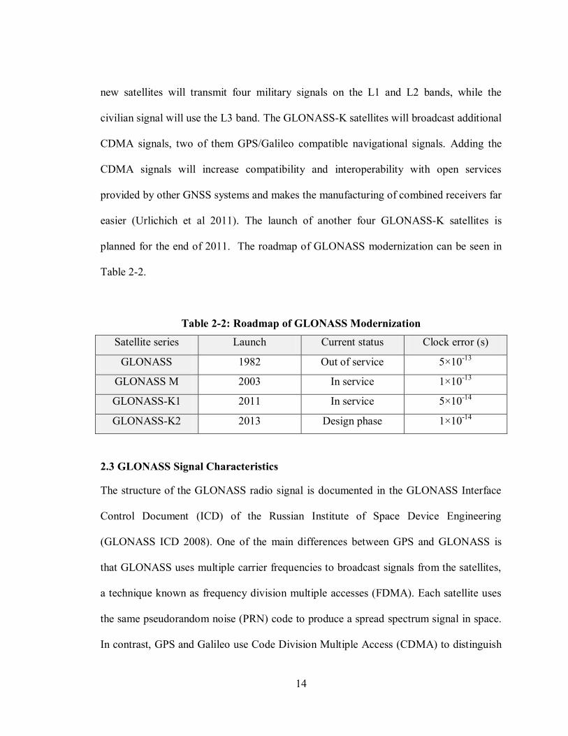
14
new satellites will transmit four military signals on the L1 and L2 bands, while the
civilian signal will use the L3 band. The GLONASS-K satellites will broadcast additional
CDMA signals, two of them GPS/Galileo compatible navigational signals. Adding the
CDMA signals will increase compatibility and interoperability with open services
provided by other GNSS systems and makes the manufacturing of combined receivers far
easier (Urlichich et al 2011). The launch of another four GLONASS-K satellites is
planned for the end of 2011. The roadmap of GLONASS modernization can be seen in
Table 2-2.
Table 2-2: Roadmap of GLONASS Modernization
Satellite series Launch Current status Clock error (s)
GLONASS 1982 Out of service 5×10-13
GLONASS M 2003 In service 1×10-13
GLONASS-K1 2011 In service 5×10-14
GLONASS-K2 2013 Design phase 1×10-14
2.3 GLONASS Signal Characteristics
The structure of the GLONASS radio signal is documented in the GLONASS Interface
Control Document (ICD) of the Russian Institute of Space Device Engineering
(GLONASS ICD 2008). One of the main differences between GPS and GLONASS is
that GLONASS uses multiple carrier frequencies to broadcast signals from the satellites,
a technique known as frequency division multiple accesses (FDMA). Each satellite uses
the same pseudorandom noise (PRN) code to produce a spread spectrum signal in space.
In contrast, GPS and Galileo use Code Division Multiple Access (CDMA) to distinguish

15
between the satellites. Using the FDMA technique results in better interference rejection
for narrow-band interference signals compared to CDMA techniques. A narrow band
interference source can disrupt only one FDMA GLONASS signal, whereas it can disrupt
all CDMA GPS signals. One disadvantage of GLONASS is the use of FDMA which
requires more spectrum than the CDMA used in GPS. GLONASS satellites transmit C/A-
code and P-code on L1 between 1602.0 and 1615.5 MHz and on L2 between 1246.0 and
1256.5 MHz
2.3.1 GLONASS RF Frequency Plan
According to GLONASS ICD (2008), the nominal values of L1 and L2 carrier
frequencies are defined by the following expressions:
1 01 1,kf f K f (2.1)
2 02 2 ,kf f K f (2.2)
K is a frequency number (frequency channel) of the signals transmitted by GLONASS
satellites in the L1 and L2 sub-bands:
f01 = 1602 MHz; Δf1 = 562.5 kHz, for sub-band L1
f02 = 1246 MHz; Δf2 = 437.5 kHz, for sub-band L2
According to GLONASS ICD (2008), the carrier frequencies L1 and L2 are generated
from a common onboard time/frequency standard in each satellite. The nominal value of
this frequency is equal to 5.0 MHz
16
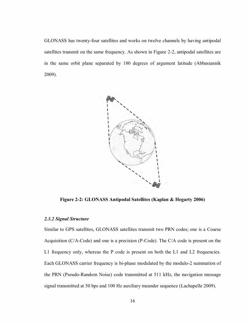
GLONASS has twenty-four satellites and works on twelve channels by having antipodal
satellites transmit on the same frequency. As shown in Figure 2-2, antipodal satellites are
in the same orbit plane separated by 180 degrees of argument latitude (Abbasiannik
2009).
Figure 2-2: GLONASS Antipodal Satellites (Kaplan & Hegarty 2006)
2.3.2 Signal Structure
Similar to GPS satellites, GLONASS satellites transmit two PRN codes; one is a Coarse
Acquisition (C/A-Code) and one is a precision (P-Code). The C/A code is present on the
L1 frequency only, whereas the P code is present on both the L1 and L2 frequencies.
Each GLONASS carrier frequency is bi-phase modulated by the modulo-2 summation of
the PRN (Pseudo-Random Noise) code transmitted at 511 kHz, the navigation message
signal transmitted at 50 bps and 100 Hz auxiliary meander sequence (Lachapelle 2009).

17
Referring to Urlichich et al (2011), GLONASS-K satellites broadcast new CDMA signals
in the L3 band on a carrier frequency of 1202.025 MHz
The ranging code chipping rate for the CDMA signal is 10.23 mega chips per second
with a period of 1 millisecond. The new signal uses a quadrature phase-shift keying
(QPSK) modulation technique with an in-phase data channel and a quadrature pilot
channel. The signal spectrum is shown in Figure 2-3.
Figure 2-3: L3 CDMA Signal Spectrum (Urlichich et al 2011)
2.3.2.1 Standard Accuracy Ranging Code (C/A-Code)
The C/A code is a 511 bit binary sequence that is modulated onto the carrier frequency at
a chipping rate of 0.511 MHz and thus repeats every millisecond (Kaplan & Hegarty
2006). It is derived from the seventh bit of a nine-bit shift register. The code is described
by the irreducible polynomial 1 + x5 + x7. The initial state is defined as each bit
containing the value ’1’ (GLONASS ICD 2008). A simplified block-diagram of the PR
ranging code is given in Figure 2-4.

18
2.3.2.2 High Accuracy Ranging Code (P-Code)
The GLONASS has a P-code. It is a 5.11 million bits long binary sequence that is
modulated onto the carrier frequency at a chipping rate of 5.11 MHz and thus repeats
every second (Kaplan & Hegarty 2006). The P-code is not used in this thesis.
Figure 2-4: GLONASS C/A-code Generation (GLONASS ICD 2008)
2.3.3 Intra-system Interference
According to GLONASS ICD (2008), the Intra-system interference is caused by the
inter-correlation properties of the ranging codes and the FDMA technique used in
GLONASS. The interference happens in the receiver between the navigation signal
transmitted on frequency channel K=n and signals transmitted on frequency channels
K=n+1 and K=n-1. This interference is conditional on the simultaneous visibility of the
satellites with adjacent frequencies.

19
2.3.4 GLONASS Navigation Message
The navigation message contains immediate and non-immediate data. It is broadcast from
GLONASS satellites at a rate of 50 bps to provide users with requisite data for
positioning, timing and planning observations (GLONASS ICD 2008). The GLONASS
navigation data structure is described in detail in GLONASS ICD (2008) and is not
reviewed here.
The immediate data relates to the GLONASS satellite which broadcasts a given
navigation signal that includes the enumeration of the satellite time marks, the difference
between the onboard time scale of the satellite and GLONASS time, the relative
difference between the carrier frequency of the satellite and its nominal value and
ephemeris parameters and the other parameters.
The non-immediate data contains an almanac of the system including: Data on the status
of all satellites within the space segment (status almanac), coarse corrections to the
onboard time scale of each satellite relative to GLONASS time (phase almanac), the
orbital parameters of all satellites within the space segment (orbit almanac) and
correction to GLONASS time relative to UTC(SU) and the other parameters (GLONASS
ICD 2008).
2.4 Comparison between GPS and GLONASS
This section provides a comparison of GPS and GLONASS. When combining GPS and
GLONASS, it is important to understand the differences between the two systems. The
major difference between GPS and GLONASS can be found in the constellations, the
time reference system, the coordinate reference system, and the signal multiplexing
20
technique. The difference between GPS and GLONASS space segments (constellation)
was discussed in detail in Section 2.2.1. The following sections discuss the GPS and
GLONASS time and coordinates systems.
2.4.1 Time Reference Systems
GPS and GLONASS have their own independent time systems; therefore, the
transformation from GLONASS time into GPS time cannot be performed easily. The
difference between the two time scales must be taken into account in the combined
GPS/GLONASS data processing.
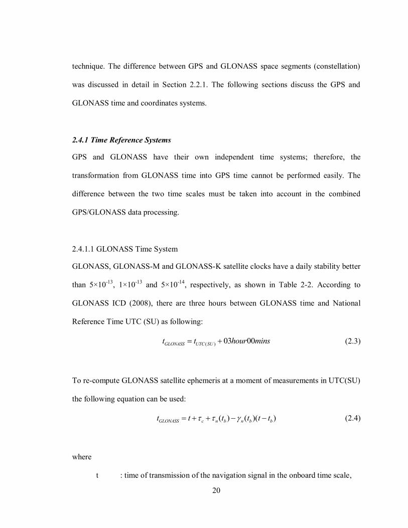
2.4.1.1 GLONASS Time System
GLONASS, GLONASS-M and GLONASS-K satellite clocks have a daily stability better
than 5×10-13, 1×10-13 and 5×10-14, respectively, as shown in Table 2-2. According to
GLONASS ICD (2008), there are three hours between GLONASS time and National
Reference Time UTC (SU) as following:
( ) 03 00GLONASS UTC SUt t hour mins (2.3)
To re-compute GLONASS satellite ephemeris at a moment of measurements in UTC(SU)
the following equation can be used:
( ) ( )( )GLONASS c n b n b bt t t t t t (2.4)
where
t : time of transmission of the navigation signal in the onboard time scale,

21
τc : GLONASS time scale correction to UTC (SU) time,
tb : index of a time interval within current day,
τn(tb) : correction to nth satellite time relative to GLONASS time at time tb,
γn(tb) : relative deviation of predicted carrier frequency value of n-satellite from
nominal value at time tb
GLONASS-M satellites transmit the difference between the GPS and GLONASS time
scale (which is never more than 30 ns) (GLONASS ICD 2008).
2.4.1.2 Time Transformation
GLONASS time could be transformed into GPS time using the following formula (Cai
2009):
GPS GLONASS c u gt t (2.5)
where
( )c UTC SU GLONASSt
( )u UTC UTC SUt t
g GPS UTCt t
In combined GPS/GLONASS data processing, the differences between these time scales
must be accounted for. Otherwise, systematic errors are introduced that will affect the
combined positioning solution.

22
2.4.2 Coordinate Systems
Referring to Abbasiannik (2009), before 1993, GLONASS provided ephemeris data in
the Soviet Geodetic System 1985 (SGS-85). From August 1993 to September 2007,
GLONASS transmitted ephemeris data in the Earth Parameter System 1990 (PZ-90). PZ-
90 is similar in quality to the Earth model employed in WGS-84 used for GPS.
2.4.2.1 PZ-90 (GLONASS)
The definitions of these coordinate frames as used by GLONASS are as follows
(GLONASS ICD 2008):
the origin is Earth’s center of mass.
the z-axis is parallel to the direction of the mean North Pole according to the
mean epoch 1900 - 1905 as defined by the International Astronomical Union and
the International Association of Geodesy.
the x-axis is parallel to the direction of the Earth’s equator for the epoch 1900 -
1905, with the XOZ plane being parallel to the average zero meridian, defining
the position of the origin of the adopted longitude system.
the y-axis completes the geocentric rectangular coordinate system as a right-
handed system.
Table 2-3 defines the parameters of the associated terrestrial ellipsoid and other
geodetic constants (GLONASS ICD 2008).

23
Table 2-3: Elements of PZ-90 System
Semi-major axis 6.378136 × 10⁶ m
Earth Rotation rate 7.292115 × 10⁻⁵ rad/s
Flattening 1/298.257839303
Gravitational Constant 3.9860044 × 10¹⁴ m3/s2
2nd Zonal Coefficient 1082625.75×10-9
In June 2007, Russia decided to implement PZ-90.02. Thus, GLONASS transmits the
ephemeris starting from that period using the PZ-90.02 coordinate system. By using the
new system, the GLONASS orbit accuracy improved by 15-25% (GLONASS ICD 2008).
2.4.2.2 WGS-84 (GPS)
GPS originally employed a coordinate frame known as the World Geodetic System 1972
(WGS72). Later the reference frame changed to the World Geodetic System 1984
(WGS84). These reference frames are defined as follows (GPS ICD 2010):
the origin is Earth’s center of mass.
the z-axis is the direction of the IERS (International Earth Rotation and Reference
Systems Service) Reference Pole (IRP).
the x-axis is the intersection of the IERS Reference Meridian (IRM) and the plane
passing through the origin and normal to the Z-axis.
the y-axis completes a right-handed, Earth-Centered, Earth-Fixed orthogonal
coordinate system.

24
Table 2-4 shows four defining parameters of the associated terrestrial ellipsoid and one
value derived from them (GPS ICD 2010).
Table 2-4: Elements of WGS 84 System
Semi-major axis 6.378137 × 10⁶ m
Earth rotation rate 7.2921151467 × 10⁻⁵ rad/s
Flattening 1/298.257223563
Gravitational constant 3.986004418 × 10¹⁴ m3/s2
2nd zonal coefficient -0.484166774985 × 10⁻³
Table 2-5 summarizes key parameters of GPS and GLONASS that must be considered
when combining GPS/GLONASS data processing.

25
Table 2-5: Comparison between GPS and GLONASS
GLONASS GPS
Constellation
Number of satellite 24 32
Number of orbital plane 3 6
Orbital inclination 64.8° 55°
Orbital radius 25510 km 26560 km
Orbital altitude 19130 km 20200 km
Orbit Period 11h 15.8 min 11h 58 min
Signal
Characteristics
Multiplexing FDMA CDMA
Carrier Frequencies 1602+k×0.5625 MHz
1246+k×0.4375 MHz
1575.42 MHz
1227.60 MHz
Code Frequencies C/A code : 0.511
P code : 5.11
C/A code:1.023
P code:10.23
Broadcast ephemerides Position, velocity,
acceleration
Keplerian
elements
Coordinates System PZ-90.02 WGS-84
Time System GLONASS Time GPS Time
2.5 Advantages of Combined GPS and GLONASS
GLONASS and GPS users might find themselves having to operate in environments with
poor satellite signal reception, for example in urban or mountainous areas, during aircraft
manoeuvres, or in the presence of interference.
In such situations, the combined use of GLONASS and GPS navigation signals may
significantly improve the quality of navigation. The use of GLONASS in addition to GPS
provides significant advantages, such as:

26
increased satellite signal observations
markedly increased spatial distribution of visible satellites
reduced horizontal and vertical DOP factors
When GLONASS and GPS are combined, the following must be taken into account:
i. the different structures of the GLONASS and GPS navigation data.
ii. the differences between the coordinate systems used for GLONASS and GPS.
iii. the time scale offset between GLONASS and GPS.
The next chapter presents an overview of GNSS receiver design and discusses the GNSS
signal processing strategies used in this thesis.

27
Chapter Three: Overview of GNSS Receiver Design and Test Measures
3.1 Chapter Outline
This chapter describes GNSS receiver design and GNSS signal processing techniques
including acquisition and tracking. The chapter continues by describing the GNSS
Software Navigation Receiver (GSNRxTM) architecture used in this thesis. Then it
discusses its standard and high sensitivity processing modes. The chapter concludes by
discussing the least-squares and Kalman filter estimation techniques used and addressing
the test measures used, namely the measurement availability, the fading analysis, the
residual analysis, and the positioning accuracy, navigation solution availability and DOP.
3.2 General Overview of GNSS Receiver Architecture
The purpose of GNSS receivers is to process signals transmitted by GNSS satellites,
estimate the user-to-satellite ranges and range rates and compute a Position, Velocity and
Time (PVT) solution (Kaplan & Hegarty 2006). The high level architecture of a GNSS
receiver is illustrated in Figure 3-1. As shown in the figure, GNSS receivers consist of
four blocks: Antenna, RF front-end, local oscillator and signal processing block. The
antenna is the first element of the receiver architecture. The transmitted signal is Right
Hand Circularly Polarized (RHCP), so the antenna must be designed to receive RHCP
signals. The antenna gain pattern is an important consideration that indicates how well
the antenna performs at different centre frequencies, different polarizations and different
elevation angles. Figure 3-2 illustrates the typical gain patterns of the NovAtel antenna
GPS 702GG which can receive GPS L1 and L2, as well as GLONASS L1 and L2 signals.

28
(a) GPS L1 (b) GLONASS L1
Figure 3-2: Typical RHCP and LHCP Normalized Radiation Pattern of NovAtel Antenna GPS-702 GG for GPS L1 and GLONASS L1 Central Frequency (NovAtel
Inc. 2011)
Channel k Channel 2
Channel 1
Preamplifier Down IF Sampling Converter
IF Signal Processing
Processing Navigation
Frequency Synthesizer
Reference Oscillator
Signal Processing
RF Front-End
Local Oscillator
Antenna
Figure 3-1: High Level Architecture of GNSS Receiver (O'Driscoll & Borio 2009)

29
The pre-amplifier is the first active component after the antenna. It is often housed in the
same enclosure as the antenna element. The antenna may be capable of receiving multiple
frequency bands. Thus, there may be one pre-amplifier per frequency band of interest, or
a single pre-amplifier may cover multiple frequency bands. The primary purpose of the
preamplifier is to amplify the signal at the output of the antenna for further processing
(O'Driscoll & Borio 2009). However, it is vital that this amplifier has a very low noise
figure, hence the amplifier is usually referred to as a Low Noise Amplifier (LNA).
The RF front-end is the second part in the receiver architecture after the antenna and
LNA. The RF front-end filters, down converts and digitalizes the received signal. Each
front-end conditions the narrow band signal in each band and down converts and
digitalizes the data.
Filtering in the front-end achieves a number of objectives such as rejecting out of band
signals, reducing the noise content in the received signal and reducing the effect of
aliasing. Wide bandwidth signals, if appropriately processed, can provide higher
resolution measurements in the time domain, but come at the cost of requiring higher
sampling rates, and hence result in larger power consumption in the receiver.
Down-conversion in the front-end is the process of taking the RF signal down to some
lower frequency (either an intermediate frequency, or directly to baseband) where it is
easier to process (Kaplan & Hegarty 2006). The common form of the down-conversion is
a mixer which multiplies the RF signal by a locally generated sinusoid and filters the
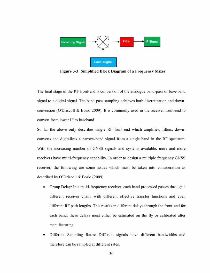
output to remove double-frequency terms (Abbasiannik 2009), as shown in Figure 3-3.
Typically filtering and down-conversion are achieved in multiple, cascaded stages due to
the difficulty in implementing a good high center frequency band-pass filter.
30
The final stage of the RF front-end is conversion of the analogue band-pass or base-band
signal to a digital signal. The band-pass sampling achieves both discretization and down-
conversion (O'Driscoll & Borio 2009). It is commonly used in the receiver front-end to
convert from lower IF to baseband.
So far the above only describes single RF front-end which amplifies, filters, down-
converts and digitalizes a narrow-band signal from a single band in the RF spectrum.
With the increasing number of GNSS signals and systems available, more and more
receivers have multi-frequency capability. In order to design a multiple frequency GNSS
receiver, the following are some issues which must be taken into consideration as
described by O’Driscoll & Borio (2009).
Group Delay: In a multi-frequency receiver, each band processed passes through a
different receiver chain, with different effective transfer functions and even
different RF path lengths. This results in different delays through the front-end for
each band, these delays must either be estimated on the fly or calibrated after
manufacturing.
Different Sampling Rates: Different signals have different bandwidths and
therefore can be sampled at different rates.
block diagram of a frequency mixer
Incoming Signal
Local Signal
Filter IF Signal
Figure 3-3: Simplified Block Diagram of a Frequency Mixer
31
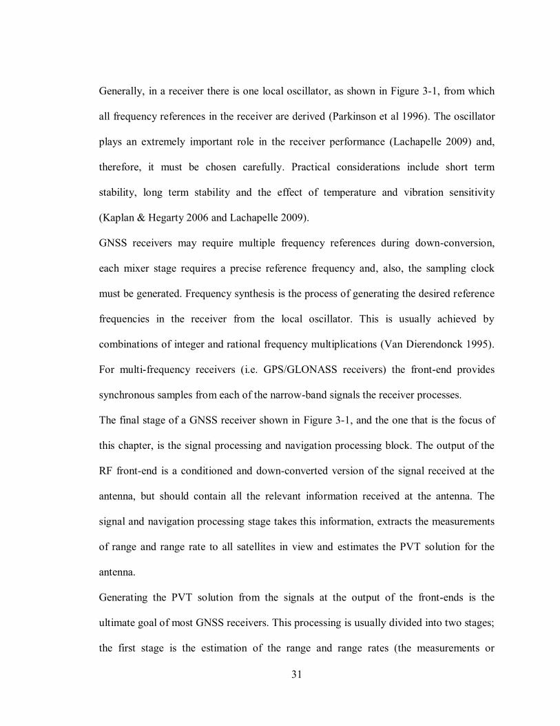
Generally, in a receiver there is one local oscillator, as shown in Figure 3-1, from which
all frequency references in the receiver are derived (Parkinson et al 1996). The oscillator
plays an extremely important role in the receiver performance (Lachapelle 2009) and,
therefore, it must be chosen carefully. Practical considerations include short term
stability, long term stability and the effect of temperature and vibration sensitivity
(Kaplan & Hegarty 2006 and Lachapelle 2009).
GNSS receivers may require multiple frequency references during down-conversion,
each mixer stage requires a precise reference frequency and, also, the sampling clock
must be generated. Frequency synthesis is the process of generating the desired reference
frequencies in the receiver from the local oscillator. This is usually achieved by
combinations of integer and rational frequency multiplications (Van Dierendonck 1995).
For multi-frequency receivers (i.e. GPS/GLONASS receivers) the front-end provides
synchronous samples from each of the narrow-band signals the receiver processes.
The final stage of a GNSS receiver shown in Figure 3-1, and the one that is the focus of
this chapter, is the signal processing and navigation processing block. The output of the
RF front-end is a conditioned and down-converted version of the signal received at the
antenna, but should contain all the relevant information received at the antenna. The
signal and navigation processing stage takes this information, extracts the measurements
of range and range rate to all satellites in view and estimates the PVT solution for the
antenna.
Generating the PVT solution from the signals at the output of the front-ends is the
ultimate goal of most GNSS receivers. This processing is usually divided into two stages;
the first stage is the estimation of the range and range rates (the measurements or

32
observations) to each satellite using the known signal structure and the second is the
estimation of the user`s position, velocity and time information using these observations.
In the GNSS receiver the signal processing can be divided into the following stages:
1. Signal Acquisition: This involves detection of the signals from satellites in view
and provides a rough estimation of the code delay and of the Doppler frequency
of the incoming signal.
2. Signal Tracking: This follows acquisition and is a recursive estimation process
that maintains continually updated estimates of some critical signal parameters.
3.2.1 Signal Acquisition
The purpose of the acquisition stage is to detect which signals are present at the output of
the front-end and to coarsely estimate sufficient signals parameters to facilitate signal
tracking. Once a signal is detected, the necessary parameters can be obtained and passed
to the signal tracking process, which is described in the next section.
Following O’Driscoll & Borio (2009), the signal model for the ith signal at the output of
the GNSS receiver front-end is given by
.
[ ] 2 1 cos 2i i i s i s IF d s ir n C h n f f f f nT n
(3.1)
where
x [n] : is the digitalized version of the continuous signal x(t) (i.e. x[n] = x(nTs),
Ci : is the filtered and quantized signal power,

33
hi(t) : is the combined data, secondary code, PRN code and sub-carrier signal,
( ) ( ) ( ) ( )i i i ih t d t s t c t (3.2)
fs : is the sampling frequency,
τi, : is the time delay and rate of change of time delay at t=0,
fIF : is the intermediate frequency,
θi : is the carrier phase,
: is the coloured Gaussian noise process that results from passing a white
noise process through the front-end and quantizing it.
The Doppler is related to the rate of change of time delay by
.
id if f (3.3)
where
fi : is the center frequency of the transmitted signal (e.g. 1575.42 for GPS
L1)
According to the above model, the signal is parameterized by the following:
1. the satellite number (SVN) : i
2. the carrier power : C
3. the time delay : τi (The Code Delay)
4. the rate of change of time delay : (The Carrier Doppler)
5. the Carrier phase : θ
.
i
.
i

34
The time delay and the carrier Doppler need to be estimated during acquisition. The
acquisition process has a two-dimensional search space, one dimension corresponding to
the PRN code delay, the other to the Doppler frequency. Typically there are three modes
for acquisition processing: cold, warm and hot modes. The receiver starts in cold mode,
since no prior information about the signal parameters is available. In cold mode, the SVs
are searched sequentially. The correlator outputs of each satellite are evaluated over a
grid of different code delays and Doppler frequencies. Once the carrier wave and pseudo-
ranging code are properly found, the de-spreading operation reduces the bandwidth of the
signal but the noise is effectively unchanged. Therefore, the signal is contained in a
narrow bandwidth while the noise power remains spread over a large bandwidth as
shown in Figure 3-4.
Figure 3-4: Sample Correlation Function
The warm start mode functions when the receiver has some knowledge such as almanacs,
and last known position and a rough estimate of time (Kaplan & Hegarty 2006). Thus, it
can choose most likely satellites to search. The last mode is the hot start mode. It

35
functions when the receiver has a recent position, time and ephemeris information
available, and already knows the satellites in view.
Bao & Tsui (2000) presented three acquisition methods: The cell-by-cell search, the fast
Fourier transformation (FFT), and the delay and multiplication method for GNSS signal
acquisition. The delay and multiplication method is faster than the FFT method but in the
case of weak signals, it has a lower performance. Therefore, there is a trade-off between
speed and sensitivity (Abbasiannik 2009). In the case of a strong received signal (i.e. high
signal to noise ratio), the fast low-sensitivity acquisition can be used and can provide
acceptable performance. If, however, the signal is weak (i.e. low signal to noise ratio), the
FFT method should be employed, as it can achieve increased signal sensitivity (Bao &
Tsui 2000).
3.2.2 Signal Tracking
The signal tracking process consists of two separate loops to estimate the code delay and
carrier frequency and phase. The Delay Lock Loop (DLL) is used to estimate the code
delay and the Carrier Lock Loop (CLL) is used to estimate the carrier phase and
frequency. The DLL estimates the code phase of the ranging code being tracked while the
CLL tracks the incoming carrier phase via a phase lock loop (PLL) or a carrier frequency
via a frequency lock loop (FLL). The two tracking loops are coupled in the sense that the
DLL requires a precise estimate of the incoming carrier frequency which the CLL can
provide and, similarly, the CLL requires a reasonable estimate of the code phase.
Figure 3-5 shows a general view of a tracking loop. Discriminators, loop filters, and
signal generators are the basic components of a tracking loop. These components are not

36
reviewed in this thesis, however detailed discussions can be found in different references
such as: Abbasiannik (2009), Bao & Tsui (2000), Kaplan & Hegarty (2006), O'Driscoll &
Borio (2009), Parkinson et al (1996) and Van Dierendonck (1995).
3.3 GNSS Software Receivers – GSNRx™
The main objective of a software receiver is to replace the data processing implemented
in hardware with software, as well as to sample the analog input signal as close to the
antenna as possible. Thus, in the case where all the signal processing is done in software,
the hardware is reduced to the minimum. One advantage of a software receiver is the
flexibility for adapting to new signals and frequencies; in a software receiver, an update
can easily be performed by changing some parameters and algorithms while a standard
hardware receiver would require total re-development.
Updating the above capabilities may become even more important in the future as the
world of satellite navigation is incomplete e.g. Galileo and Compass. A state of the art
software receiver capable of processing both GPS and GLONASS in standard or high
sensitivity modes is used in this thesis. The digitized data was post-processed in two
modes (standard and assisted HS GNSS) using the PLAN group software receiver
Figure 3-5: A Generic Tracking Loop (Kaplan & Hegarty 2006)
Incoming Signal
Signal Generator
Loop Filter Error in generated signal
Generated Signal
+
-
Discriminator
Estimate of generated signal
error

37
GSNRx™ (Petovello et al 2008). The following sections discuss the GSNRx™
architecture in standard and high sensitivity mode.
3.3.1 Overview of GSNRxTM
The GSNRx™ is a C++ class-based GNSS receiver software program developed by the
Position, Location and Navigation (PLAN) Group at the University of Calgary. This
software is developed for a GPS L1 C/A signal which is capable of processing the raw
samples from RF front-end and generating measurements to be used in other data
processing programs (Petovello et al 2008).
3.3.2 GSNRxTM Software Receiver Architecture
The general architecture adopted for the GSNRx™ software receiver is shown in
Figure 3-6 (Petovello et al 2008). The GSNRxTM is a class-based program as discussed
above, and its architecture will be described in terms of objects. According to Petovello et
al (2008), the main objects are shown in Figure 3-6.
The software receiver contains six objects: The sample source, the signal, the channel, the
satellite, the Doppler Removal and Correlator (DRC) and the processing manager. All
these objects are described in detail in Petovello et al (2008). The main objects are
described briefly below.

38
Figure 3-6: General Software Architecture of GSNRx™ (Petovello et al 2008)
The first object is the sample source as shown in Figure 3-6. This provides a stream of
samples from some sample source to the signal processing objects. The IF data samples
can be obtained from any practical sources e.g., read from files in post-mission or load
directly from an analog to digital converter in real-time. The sample object can handle
real or complex samples.
The signal object is not shown in Figure 3-6; it contains the parameters of the signal such
as carrier frequency and a ranging code. An example of a signal would be the GPS L1
C/A code, the Galileo E1b code or the Galileo E1c code.
The channel object is responsible for tracking one or more signals (Petovello et al 2008).
The inputs of the channel object are the correlator outputs from the DRC object
(described below).

39
As shown in Figure 3-6, the satellite object contains one or more of the channel objects.
Satellite objects are responsible for handling satellite-specific information such as
different ephemeris messages from different channels.
The DRC operations in the GSNRxTM for a given signal are performed by the DRC
object. The input to the DRC is the sample source and the corresponding signal
information from the channels. The outputs are the correlator values.
Finally, the processing manager object manages the relationships between the channels,
signals and sample sources. The processing manager has the ability to determine what
DRC objects are used for processing. “One advantage of this object is that the processing
manager allows highly optimized processing to take place without any modifications to
the rest of the code” (Petovello et al 2008).
Figure 3-7 shows the interaction between the processing manager and the objects
discussed above. “It starts by creating the necessary objects and composes the receiver.
The receiver object is informed of what sample sources are available and is also given
access to the processing manager. The receiver then creates (allocates) satellite objects
as needed based on assumed satellite visibility. As satellite objects are created,
information about their channels (and corresponding signals) are passed to the
processing manager, which is responsible for maintaining the relationships amongst the
sample sources, signals and DRC objects. Similarly, as satellites are removed (e.g.,
because they fall below the local horizon), they are removed from the receiver and the
processing manager is informed accordingly” (Petovello et al 2008).

40
Figure 3-7: Interaction of Processing Manager and Associated Objects (Petovello et al 2008)
3.3.3 GSNRx™ Standard versus High Sensitivity Mode
GSNRxTM has two operation modes: The standard mode and the high sensitivity mode.
Figure 3-8 shows the architecture of the GSNRx-hsTM. In standard mode, a Kalman filter
tracking strategy is active and the cascaded vector tracking is utilized. Standard vector
tracking and ultra-tight tracking are discussed by Lin et al (2011).
In high-sensitivity mode, the block processing strategy is active. The outputs from block
processing are used for generating the pseudorange and pseudorange rate measurements
for the navigation solution (Lin et al 2011). The local signal generators are then updated
by the filtered pseudorange and pseudorange rate values from the navigation filter.
External data bit aiding is used to permit long coherent integration times for noise and
multipath, while external ephemeris is used for navigation solution. The FFT parallel-

41
frequency-based correlation method is used to generate correlation/accumulation more
efficiently in the frequency domain (Lin et al 2011).
Figure 3-8: Architecture of GSNRx-hsTM (Lin et al 2011)
3.3.4 Assisted High Sensitivity GSNRxTM
The assisted HS GNSS receiver architecture used in this work is shown in Figure 3-9.
There are a number of notable changes from the standard receiver architecture that are
highlighted in red in Figure 3-9. These are discussed in more detail below.
Assistance information is provided in the form of broadcast ephemerides, raw data bits,
and a nominal trajectory (position and velocity) that would normally be generated by the
receiver as discussed above. It is the same as for the GSNRx-hsTM described above; at
each measurement epoch the receiver uses the nominal position and velocity in
conjunction with the ephemerides to compute the nominal pseudorange and pseudorange
rate for each satellite in view.

42
Figure 3-9: Assisted HS Receiver Architecture
These parameters are passed to the signal processing channels. Each channel evaluates a
grid of correlators around the nominal pseudorange (code) and pseudorange rate
(Doppler) values. The data bits are wiped off using the assistance information to permit
long coherent integration times. For each signal tracked, the correlator grid is used to
estimate code and Doppler offsets relative to the nominal values. These estimates are then
used to generate accurate pseudorange and Doppler estimates.
The number of correlators used, and the spacing of these correlators in the code and
frequency domains are completely configurable. A sample correlation grid computed
during live data processing is illustrated in Figure 3-10. Measurements are generated by
choosing the three correlators nearest the peak in the search space and using a quadratic
fit to determine a better estimate of the peak location (O'Driscoll & Borio 2009).

43
Figure 3-10: Sample Grid of Correlator Points Computed
The assisted HS receiver is initialised in static mode in an open sky setting during which
reliable clock bias and drift estimates are derived. A high quality OCXO was used during
this initial test to ensure that the clock drift did not change significantly over the period of
the test. The clock bias during the test is updated using the clock drift estimate.
Note that this architecture is a generalization of the vector-based architecture (Lin et al
2011 and Petovello & Lachapelle 2006), where the navigation solution used to aid the
signal processing can be provided by an external reference.
3.4 Estimation Methods Used
Least-squares and Kalman filter estimation techniques are used to calculate the user
position in this thesis. In static tests, a least-squares approach is used to calculate the
navigation solution. In kinematic test, a least-squares and Kalman filter approach is used
to calculate the navigation solutions. The least-squares approach will be discussed first
and followed by an explanation of the Kalman filtering estimation method.

44
3.4.1 Least-Squares Approach
The GPS/GLONASS raw data can be post-processed using a parametric least-squares
technique with positions fixed to the known test locations. The main concept of the least-
squares is to minimize a specific quadratic form, essentially by making the sum of the
squares of the weighted residuals as small as possible (Petovello 2009).
The least-squares navigation solution was accomplished using C3NavG2™, a software
package developed at the University of Calgary. C3NavG2™ is a C program that processes
GPS and/or GLONASS pseudorange and Doppler data in both static and kinematic
modes in an epoch-by-epoch mode to determine position and velocity in either single
point and differential mode. The program also allows carrier smoothing of pseudorange,
differential positioning, and height fixing. A discussion of the least-squares estimation
technique will follow.
The linearized equation that relates GLONASS or GPS pseudorange measurements to the
unknown user position and clock offset is
(3.4)
where
: is the vector of pseudorange measurement residuals (the vector offset
of the measured and calculated pseudorange measurements).
H : is the design matrix containing the linear relationships between the
pseudorange measurements and the user position and clock offset.
: is the user position and clock offset correction vector.
v H x
v
x

45
To estimate the receiver position and clock offset with respect to GPS or GLONASS
time, the user state vector is given by
GPS GLONASSx x y z t t (3.5)
where
∆x : is the position deviation in the X direction
∆y : is the position deviation in the Y direction
∆z : is the position deviation in the Z direction
∆tGPS : is the receiver clock offset with respect to GPS
∆tGLONASS : is the receiver clock offset with respect to GLONASS time
The design matrix H is given by
1 1 1
2 2 2
1 01 0
: : : : :0 1
SV SV SVx y zSV SV SVx y z
SVn SVn SVnx y z
H
(3.6)
The term represents the direction cosines from the receiver to satellite N in the X,
Y and Z directions. The pseudorange residual vector is given by
(3.7)
, ,SVNx y z
1 1
2 2
:
c m
c m
cn mn
PR PRPR PR
v
PR PR

46
where PRcn is the nth calculated pseudorange measurement based on the satellite position
and the estimated receiver position, PRmn is the nth measured pseudorange.
The least-squares solution that minimizes the residuals of the user position is given by
, (3.8)
where W is the weight matrix.
Assuming that the pseudorange measurements are independent and have a Gaussian
distribution, the weight matrix for N GPS and R GLONASS satellites is given by
(3.9)
where
: is the standard deviation for the nth GPS satellite
: is the standard deviation for the rth GLONASS satellite
Since the low elevation angle satellites usually contain higher noise levels because the
signals travel through more atmosphere than higher elevation satellites, the lower
1T Tx H WH H W v
21
22
2
21
2
1 / 0 0 0 0 0 00 1 / 0 0 0 0 00 0 : 0 0 0 00 0 0 1 / 0 0 00 0 0 0 1 / 0 00 0 0 0 0 : 00 0 0 0 0 0 1 /
GPS
GPS
GPSN
Glo
GloR
W
GPSn
Glor

47
elevation satellites should be weighted less than the higher elevation satellites. The
weighting method based on satellite elevation angle is used in the static tests presented in
Chapter 4. In this weighting method, the standard deviations for measurements made at
the zenith are scaled by 1/sin (e) where e is the satellite elevation angle.
In urban canyon environments, satellite masking by tall buildings and trees is an issue as
discussed in Chapter 1. Often only satellites with high elevation angles can be observed.
And the estimated position in urban environment is mainly corrupted by multipath and
signal diffraction. Another weighting method linking the measured C/N0 to the variance
of the observation is used in the dynamic tests presented in Chapter 5. In this method, the
standard deviations for measurements made at the zenith are scaled by Re0Re0
//
ference
ceivedC NC N
where Re0/ ferenceC N is chosen in this thesis to be equal to 50 dB-Hz, which represents the
typical value of C/N0 in open sky conditions.
The new residual vector x in Equation (3.8) is iteratively generated and added to the
estimated position and clock vector. The updated value will be used as a new estimate for
the next iteration. The iteration will continue until the norm of the residual vector x
converges to a desired value.
According to Petovello (2009), to relate pseudorange errors to position and clock error,
several geometry factors are introduced which are also referred to as Dilution of
Precision (DOP) parameters. The DOP parameters are obtained by taking the covariance
of both sides of Equation (3.8) as:
(3.10) 1TCov x H WH Cov v

48
Next, (HTWH)-1 is written as a full matrix as:
(3.11)
The DOP parameters are expressed in terms of the elements of (HTWH)-1 as follows:
11 22 33PDOP D D D (3.12)
33VDOP D (3.13)
11 22HDOP D D (3.14)
where P stands for position, V for vertical and H for horizontal.
3.4.2 Kalman Filtering Approach
Kalman filtering is a useful technique for estimating the state of a system given a
previous state and external measurements of the state variables. The Kalman filter
extends the concept of least-squares to include knowledge of how the state vector
behaves in time (Petovello 2009).
The Kalman filter estimates the process state at some time and then obtains feedback in
the form of (noisy) measurements (Grewal & Andrews 2001). Thus, the equations for the
Kalman filter fall into two groups: Time update equations and measurement update
11 12 13 14
1 21 22 23 24
31 32 33 34
41 42 43 44
T
D D D DD D D D
H WHD D D DD D D D

49
equations. The time update equations use the current state and error covariance to
calculate the a priori estimates for the next time step. The measurement update equations
are responsible for improving the posteriori estimate by incorporating a new
measurement into the a priori estimate. The time update equations can also be considered
as predictor equations, while the measurement update equations can be considered as
corrector equations. The Kalman filter uses a predictor-corrector algorithm to solve
numerical problems as shown in Figure 3-11.
The specific equations for the time and measurement updates are presented as follows:
(3.15)
where
xk : is the state vector.
A : is the dynamic matrix.
1k k kx Ax Bu
Correct
Measurement Update
Predict
Time Update
Figure 3-11: Algorithm of the Kalman filter (Grewal & Andrews 2001)

50
B : is the shaping matrix
uk : is the random variable representing white noise
A priori estimate error covariance matrix is
(3.16)
where
P : is the error covariance matrix
Q : is the process noise matrix
From equations (3.15) and (3.16), the time update equations represent the state and
covariance estimates forward from time step k-1 to step k.
The time update equations are
(3.17)
where
Kk : is the Kalman gain matrix.
H : is the design matrix (Observation matrix).
P : is the error covariance matrix.
R : is the measurement noise covariance matrix.
1T
k kP AP A Q
1T T
k k kK P H HP H R
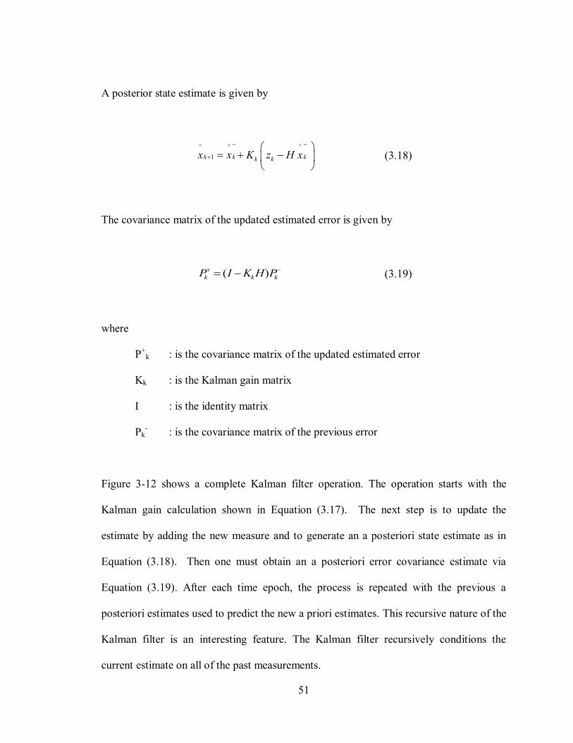
51
A posterior state estimate is given by
(3.18)
The covariance matrix of the updated estimated error is given by
(3.19)
where
P+k : is the covariance matrix of the updated estimated error
Kk : is the Kalman gain matrix
I : is the identity matrix
Pk- : is the covariance matrix of the previous error
Figure 3-12 shows a complete Kalman filter operation. The operation starts with the
Kalman gain calculation shown in Equation (3.17). The next step is to update the
estimate by adding the new measure and to generate an a posteriori state estimate as in
Equation (3.18). Then one must obtain an a posteriori error covariance estimate via
Equation (3.19). After each time epoch, the process is repeated with the previous a
posteriori estimates used to predict the new a priori estimates. This recursive nature of the
Kalman filter is an interesting feature. The Kalman filter recursively conditions the
current estimate on all of the past measurements.
^ ^ ^
1k k kk kx x K z H x
( )k k kP I K H P

52
Figure 3-12: Complete Picture of the Operation of the Kalman filter (Welch & Bishop 2001)
3.5 Test Measures
The following test measures were used to characterize measurement availability, signal
and measurement degradation and positioning accuracy and solution availability:
Measurement availability
Carrier-to-noise density ratio
Fading
Position accuracy, solution availability and dilution of precision
Each measure is explicitly defined and discussed in the following sections.

53
3.5.1 Measurement Availability
Measurement availability is a measure of the number of available measurements provided
by each test. It is a time series analysis and shows all GPS and GLONASS
measurements provided during the static or dynamic tests.
3.5.2 Carrier-to-Noise Density Ratio
Carrier-to-noise density ratio (C/N0) is a measurable value that reflects the received
signal quality (MacGougan 2003). C/N0 is a measure of the ratio of carrier power present
to noise power density measured per Hertz of bandwidth.
C/N0 is not a good estimator of signal power degradation because it is dependent on the
antenna gain pattern and the correlation process used by the receiver (MacGougan 2003).
Short-term variation in C/N0 values can be used as an estimate of signal degradation but a
better estimator of signal power degradation is fading.
3.5.3 Fading
The fading test measure is the signal strength degradation and can be measured by
differencing a rover receiver’s carrier-to-noise density ratio data with that from a
reference receiver of similar type located nearby with line-of-sight signal reception.
Fading can thus be calculated as:
0 0/ /reference roverF C N C N (3.20)

54
where F is the level of signal fade (dB), 0/ referenceC N is the carrier-to-noise density ratio at
the reference station (dB-Hz), and 0/ roverC N is the carrier-to-noise density ratio at the test
location (dB-Hz). This method assumes that there is no signal power degradation at the
reference station due to its local environment. This method also assumes that C/N0 is a
measure that reflects a linear relationship with actual signal power variation with unity
slope (MacGougan 2003).
3.5.4 Position Accuracy, Solution Availability and Dilution of Precision
To study the impact of adding GLONASS to GPS process in the receiver, it is necessary
to examine the positioning accuracy achievable with the available measurements using an
epoch-by-epoch least-squares and a Kalman filter estimation approach. In static and some
kinematic testing the height is well known, thus a height fix will be used to improve
position availability and the ability to detect measurement faults and only the horizontal
position domain will be assessed. DOP will be indicated for each solution computed to
assess the influence of solution geometry.

55
Chapter Four: Static Test Results and Analysis
4.1 Chapter Overview
This chapter provides the results of the static tests performed in two test scenarios,
namely in a suburban home and in an engineering laboratory. The methodology of these
experiments is introduced and the experimental results are presented in this chapter. The
analysis focuses on measurement availability, fading, solution availability, position
accuracy and DOP.
4.2 Static Tests
Data was collected in two test scenarios: A typical North American Wooden House (WH)
and an engineering laboratory (NavLab), the latter inside the Calgary Center for
Innovative Technologies (CCIT) building of the University of Calgary.
4.3 Methodology
Due to the severity of the attenuation and fading experienced by GNSS signals indoors,
analysis of their behaviour can be challenging. Three possible solutions can overcome
this problem. Firstly, a high sensitivity (HS) standalone/assisted GPS/GLONASS
receiver may be used (Watson 2005). Secondly, measurements from a pair of receivers, a
reference and a rover, which are synchronized to a very high accuracy, may be used
(Haddrell & Pratt 2001, Mitelman et al 2006 and Satyanarayana et al 2009). Finally,
GPS/GLONASS-like signals with a very high gain transmitter may be generated in order
to overcome the high level of attenuation caused by external walls and rooftops.

56
In these two test scenarios, the two-receiver (reference/rover) configuration is used to
process indoor GPS/GLONASS L1 C/A signals. In this method, measurements obtained
from the reference receiver placed outdoors with a clear view of the sky, can be
effectively used to compute Doppler frequency, code phase and data bits, which can be
wiped off the indoor signals, thus enabling long coherent integration for the indoor
receiver (the rover).
The data is processed with the specialised version of GSNRx™, as discussed in the
previous chapter. This reference/rover based version, called GSNRx-rr™, is a C++ class-
based GNSS receiver software program capable of processing data samples from one
reference and several rover front-ends in post-mission (Satyanarayana et al 2009). All
signals in view at the reference antenna are acquired and tracked. Approximate code
phase and Doppler frequency and navigation bits extracted from the reference signal are
used to wipe-off the code, carrier and data bits from the signals collected from the rover
antenna.
A grid of correlator values are computed at a variety of code phase and Doppler offsets
around the reference values. This configuration is illustrated schematically in Figure 4-1.

57
Figure 4-1: Schematic of GSNRx-rr™
The use of the reference values for data, code and carrier means that the rover data can be
correlated over very long coherent integration times, permitting the computation of the
cross ambiguity function of the rover data even for very weak signals. Using this grid of
correlator values, various signal parameters including C/N0, delta pseudorange and delta
frequency can be computed. In these static tests, the focus is on pseudorange
measurements in a static environment, so the Doppler measurements from the reference
receiver are used directly. The correlator grid has been chosen to span +/- 2 chips around
the reference code phase in 0.1 chip increments. In this way a relatively fine level of
detail can be observed, in addition to long range multipath (greater than 1 chip delay),
should it exist.
A coherent integration time of one second was chosen. This permits the reliable
observation of signals with C/N0 values as low as 10 dB-Hz. In addition, the long
integration helps reduce the impact of cross-correlation and other RF interference
(Kaplan & Hegarty 2006). As such, the measurements generated in this configuration
RF
RF
Standard Tracking
2·
2·
2·
Code Gen………
Data Bits
Carrier Replica
Code Phase
ReferenceAntenna
RoverAntenna

58
represent a best case scenario. These parameters are not easily achievable in practice
without the aiding provided by the reference antenna (Satyanarayana et al 2009).
Once the grid of correlator values has been computed, a simple quadratic interpolation is
used to determine the location of the peak code phase. In the case that there is no
multipath, this represents a reasonable approximation to the maximum likelihood
estimate of the code phase difference between the reference and the rover. Pseudorange
difference measurements can then be made directly by scaling the code phase to units of
length. The error model adopted for this delta pseudorange measurement is given by
pPR R MP n c t (4.1)
where
∆PR : is the delta pseudorange measurement,
∆R : is the true range difference,
∆MP : is the difference between the multipath error in the reference
measurement and that in the rover measurement,
∆n : is the difference in the thermal noise contributions of the two
measurements,
c : is the speed of light,
∆tp : is the differential delay due to differences in cable lengths
connecting the reference and rover antennas to their respective
front-ends.

59
The final stage in the methodology is the computation of position solutions at the rover.
To this end, the measurements are post-processed to generate a position and clock only
(no velocity) solution using a weighted least-squares algorithm with blunder detection
and removal (Kay 1993) using C3NavG2™. The measurements are weighted using a
standard elevation-dependent model discussed in the previous Chapter. The position
solutions are computed using three separate approaches:
1. using GPS measurements only (denoted GPS),
2. using both GPS and GLONASS measurements, and estimating the
GPS/GLONASS time offset (denoted GLO),
3. using both GPS and GLONASS measurements and providing the system time
offset estimated from the reference measurements (denoted GG+CLK).
The results are compared in terms of solution availability, accuracy and geometry (HDOP
and VDOP).
4.4 Test Setup and Description
Data was collected using five National Instruments PXI-5661 front-ends, in two separate
chassis, and two NovAtel GPS702-GG model antennas. The NovAtel GPS702-GG
antenna can receive GPS and GLONASS L1 and L2 signals. The first antenna was
placed on the rooftop with a clear view of the sky and used as a reference, while the
second one was placed in a degraded environment (the rover). Figure 4-2 shows the test
setup adopted for collecting synchronous GPS/GLONASS L1 C/A signals. The reference
signal was passed through a low noise amplifier followed by a splitter where it was
divided into three signals. One of these signals was passed to the first NI chassis, where it

60
served as the source of reference GPS data. The other two were passed to the second NI
chassis, one of which served as a source of the GLONASS reference data, the second of
which was used to provide precise sample level synchronization between the two chassis.
The front-ends used to collect this data were driven by the same local oscillator, thereby
ensuring that both reference and rover measurements were subject to the same clock bias
and drift effects. In the front-ends, the signals were sampled and down-converted into the
desired intermediate frequency.
In the case of the rover antenna, the same setup was used, but without the extra
synchronization signal. Digitized samples from the NI system were stored on an external
hard drive and later processed with the GSNRx-rr™. Figure 4-3 shows the experimental
setup in the WH test scenario.
Roof Antenna
Amplifier
NI – Chassis 1
Channel 1 (GPS)
Channel 2 Clk
Channel 3 (GPS)
Indoor Antenna
Amplifier
NI – Chassis 2
Channel 1 (GLO)
Channel 2 (GPS) Clk
Channel 3 (GLO)
Splitter
Splitter
Figure 4-2: Test Setup Adopted for Collecting Synchronous Live GPS/GLONASS L1 C/A Signals

61
(a) Two NI Front-ends (b) Experimental Connections
Figure 4-3: Experimental Setup for WH Test
The specifications of the digitized signals for the two test scenarios, typical North
American WH and NavLab, are shown in Table 4-1.
Table 4-1: Settings Adopted for the Data Collection
Parameters GPS Signal GLONASS Signal
Sampling Frequency (MHz)
5 (WH) 12.5 (NavLab) 12.5
IF Frequency (MHz) 0.42 0
Sampling Complex Complex
Quantization Bits 16 16
4.5 Experimental Results and Analysis
In this section, the results obtained using the GSNRx™ receiver for the two experiments
described above are detailed. The section includes results from the combined GPS and
GLONASS in terms of detection, measurement and position accuracy.

62
4.5.1 Wooden House (WH) Test Results
This type of wooden house represents a relatively benign indoor environment, but still
poses significant challenges to standard receivers. Signal attenuation was of the order of 5
to 25 dB, with most signals attenuated by less than 15 dB. The locations of the reference
and rover antennas are shown in Figure 4-4. The test lasted just under 10 minutes, with a
1 Hz solution rate; a total of 564 solutions were possible.
(a) Location of Reference Antenna for the
WH Test (b) Location of Rover Antenna for the WH
Test Figure 4-4: Locations of the Reference and Rover Antennas for WH Test
4.5.1.1 Measurement Availability
Signal availability for the receiver was good for the test period. The skyplot of the
satellites visible at the start of the test is shown in Figure 4-5. There were eleven GPS and
six GLONASS satellites in view. Since the test duration was only 10 minutes, there was
little variation in geometry for the duration of the test.
Rover Antenna

63
Figure 4-5: Skyplot for the Start of the WH Test
The number of satellites tracked by the rover receiver on the main floor of the WH test is
shown in Figure 4-6. The rover receiver was able to track nine GPS and four GLONASS
satellite during the test. The statistics concerning the number of satellites tracked are
shown in Table 4-2. The combination between GPS and GLONASS clearly results in
more measurements than using only GPS or GLONASS. The DOP corresponding to the
useable measurements is discussed in 4.5.1.5.

64
Figure 4-6: WH Test Signal Availability
Table 4-2: WH Test – Satellites Availability Statistics
Parameters GPS GLONASS GPS+GLO
Mean 7.6 2.3 9.9
Maximum 9 4 12
Minimum 3 0 6
σ 0.9 0.5 0.8
Some sample correlator outputs are shown in Figure 4-7 and Figure 4-8. The impact of
fading is clearly visible in each of these plots, while the effect of the instantaneous
multipath is not readily discernable. A visual inspection shows one clear peak in each
epoch, indicating that the multipath is all close range. This is to be expected given that
most of the significant reflectors are within a few metres or tens of metres of the rover
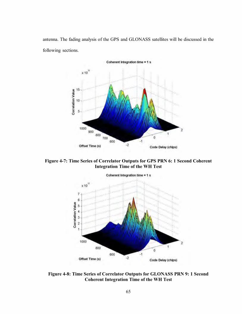
65
antenna. The fading analysis of the GPS and GLONASS satellites will be discussed in the
following sections.
Figure 4-7: Time Series of Correlator Outputs for GPS PRN 6: 1 Second Coherent Integration Time of the WH Test
Figure 4-8: Time Series of Correlator Outputs for GLONASS PRN 9: 1 Second Coherent Integration Time of the WH Test

66
4.5.1.2 Carrier-to-Noise Density Ratio
The C/N0 estimated from the rover correlator outputs is illustrated in Figure 4-9 and
Figure 4-10 for GPS and GLONASS satellites, respectively. Both the levels and the
trends observed in the C/N0 values are very similar between GPS and GLONASS. While
the two signals are in slightly different frequency bands, the fading environment appears
very similar in each case. This is encouraging, as it suggests that the high sensitivity
processing developed for GPS in GSNRx™ is equally effective for GLONASS.
Figure 4-9: Carrier-to-Noise Density Ratio of the GPS Signals Received on the Main Floor of the WH Test.

67
Figure 4-10: Carrier-to-Noise Density Ratio of the GLONASS Signals Received on the Main Floor of the WH Test
4.5.1.3 Fading Analysis
C/N0 is not a good estimator of signal power degradation because it is dependent on the
antenna gain pattern and the correlation process used by the receiver (MacGougan 2003).
Short-term variation in C/N0 can be used as an estimate of signal degradation but fading
analysis, which was discussed in Chapter Three, is, perhaps, a better estimator. The time
series fading analysis of GPS and GLONASS satellites is illustrated in Figure 4-11 and
Figure 4-12, respectively. The signal strength degradation is due to two factors. The first
is the attenuation of the LOS signal due to propagation through material, which is often
referred to as shadowing. The second factor is constructive and destructive interference
when the signals experience interference, multipath for example. This effect is generally

68
referred to as fading. However, in this thesis, fading refers to both the shadowing effect
and the interference fading effect.
Figure 4-11: Time Series Fading Analysis of GPS Satellites for the WH Test
Figure 4-12: Time Series Fading Analysis of GLONASS Satellites for the WH Test

69
4.5.1.4 Estimated Pseudorange Error
To determine the extent to which multipath, noise, echo-only signals, and other
interference degrade the pseudorange measurements taken at the test site, the test
receiver’s raw data can be post-processed using estimation techniques in which the error
on the measurement to each satellite are estimated. This test metric is referred to as
estimated pseudorange error (EPE).
Unfortunately for this test, the true position of the rover antenna is not available. Thus, it
is not possible to directly observe the RMS errors. Figure 4-13 shows the estimated
standard deviations of the GPS and GLONASS delta pseudorange measurements as a
function of C/N0.
Figure 4-13: Delta Pseudorange Standard Deviations Versus C/N0 for the WH Test

70
Figure 4-13 was obtained by dividing the measurements into bins based on the estimated
C/N0 values. The trend of increasing standard deviation with decreasing C/N0 is to be
expected. It would also be expected that the GLONASS measurements should be noisier
than the GPS measurements, due to the lower chipping rate of the GLONASS C/A code.
As can be seen from the figure, however, the opposite appears to hold in this case.
Though, it must be acknowledged that the number of observations at the lower end of the
C/N0 scale is low, leading to a less accurate estimate of the pseudorange standard
deviation. In reality, it appears that the measurement errors in this case are approximately
the same for the two systems.
Referring to Equation (4.1), it is evident that the major contributors to the estimated
standard deviations are the rover thermal noise errors and the temporal variation of the
rover multipath errors. The true range difference ∆R varies by only a few decimetres at
most and does not contribute to the standard deviations. The ∆tp term should be constant
throughout the test.
4.5.1.5 Position Accuracy, Solution Availability and Dilution of Precision
A scatter plot of the horizontal positions computed is given in Figure 4-14. Recall that the
three solutions correspond to: 1) GPS only measurements, 2) GPS plus GLONASS
measurements, with estimation of the system time offset, 3) GPS plus GLONASS
measurements with provision of the system time offset.

71
Figure 4-14: Scatter Plot of Horizontal Positions Computed for the WH Test. The Origin is given by the Mean Value of the GG+CLK Case
Figure 4-15 shows the time series analysis of the position errors for WH test. The true
position of the rover antenna is not available. Thus, the reference position was obtained
by the Mean Value of the GG+CLK case. According to the following results, the position
errors vary within 15 m of the reference position. For this environment, all three
approaches yielded almost acceptable position errors during the experiment time.

72
Figure 4-15: Time Series Analysis of Positions Errors Computed for the WH Test. The Reference Position is given by the Mean Value of the GG+CLK Case
Figure 4-16 shows the percentage of the time the least-squares algorithm was able to
converge on a valid solution. Here the position solution was obtained by setting a
minimum C/N0 threshold. Measurements for which the C/N0 was below the threshold
were not considered by the navigation solution. Thus, the performance of receivers with
different levels of sensitivity can be compared, with the caveat that the measurements
generated here are less susceptible to interference than less sensitive receivers due to the
1s integration time. For this environment, all three approaches yielded almost 100 %
solution availability for all reasonable levels of receiver sensitivity.

73
Figure 4-16: Percentage Solution Availability Versus Receiver Sensitivity for the WH Test (Note That 100 % Availability is Seen in Most Cases).
The impact of adding GLONASS to GPS satellites on geometry is evaluated by
comparing the HDOP and VDOP for each of the three cases. Figure 4-17 and Figure 4-18
show the mean, maximum and minimum HDOP and VDOP values, respectively,
observed in each case. There appears to be an approximately 30 % improvement in
HDOP when adding GLONASS in this case.
Figure 4-19 and Figure 4-20 show the standard deviations in the horizontal and vertical
positions for each of the three processing cases as a function of receiver sensitivity. There
is very little difference between the GPS only and the GPS plus GLONASS solutions in
this case, with some improvement in the vertical positions when GLONASS is added.

74
Figure 4-17: Mean, Maximum and Minimum HDOP Versus Receiver Sensitivity for the WH Test. The Continuous Lines Represent the Mean Value; the Error Bars
Report the Maximum and Minimum
Figure 4-18: Mean, Maximum and Minimum VDOP Versus Receiver Sensitivity for the WH Test. The Continuous Lines Represent the Mean Value; the Error Bars
Report the Maximum and Minimum

75
Figure 4-19: Standard Deviations of the Horizontal Position Error Versus Receiver Sensitivity for the WH Test
Figure 4-20: Standard Deviations of the Vertical Position Errors Versus Receiver Sensitivity for the WH Test

76
While the above analysis was based on an integration time of 1s, this is not always
practical. The receiver C/N0 threshold can be approximated using a simple rule of thumb
which states that the SNR at the correlator outputs should be greater than 10 dB for
reliable detection. The C/N0 and SNR can be approximately related by the equation:
02 /SNR C N T (4.2)
A plot of required integration time versus C/N0 is shown in Figure 4-21.
Figure 4-21: Required Integration Time Versus Receiver C/N0 Threshold

77
The horizontal and vertical standard deviations of position errors analyses were repeated
in terms of coherent integration time. Figure 4-22 and Figure 4-23 show the horizontal
and vertical standard deviations of position errors versus coherent integration time. The
position solution was obtained by setting a different coherent integration time. Thus, the
performance of receivers with different integration time can be compared. For this
environment, all three approaches yielded almost acceptable standard deviations of
position errors for all reasonable levels of coherent integration time. According to the
following results, there is not much improvement in terms of standard deviations of
position error value when increasing the coherent integration time more than 500 ms.
Figure 4-22: Standard Deviations of the Horizontal Positions Errors Versus Coherent Integration Time for WH Test

78
Figure 4-23: Standard Deviations of the Vertical Position Errors Versus Coherent Integration Time for WH Test
4.5.2 Engineering Laboratory Test Results
For this scenario the reference antenna was installed on the roof of the CCIT building
while the rover antenna was placed in the Navigation Laboratory (NavLab) one floor
below the roof. This represents an extremely challenging environment for GNSS signals,
with multiple reflectors at close range and a high degree of attenuation in most directions,
of the order of 15 to 45 dB. The laboratory also contains a significant amount of
electronic equipment, two pieces of which were found to produce RF interference in the
L1 band. For the purposes of this test these interferers were switched off. This test lasted
eight minutes and with a measurement rate of 1 Hz, over 460 position solutions were
generated. The locations of the reference and rover antennas are shown in Figure 4-24.
These locations are both known to within a few centimetres, which permit the

79
computation of absolute range and position errors for the purposes of comparison in the
following analysis.
(a) Location of Reference Antenna
for the NavLab Test (b) Location of Rover Antenna for the NavLab Test
Figure 4-24: Locations of the Reference and Rover Antennas for NavLab Test
4.5.2.1 Measurements Availability
The sky plot at the start of the test is shown in Figure 4-25. In this case there were nine
GPS and six GLONASS satellites in view.
Figure 4-25: Skyplot for the Start of the NavLab Test
Reference Rover

80
The number of satellites tracked by the indoor receiver in the NavLab test is shown in
Figure 4-26. The receiver was able to track seven GPS and five GLONASS satellite
signals. The statistics concerning the number of satellites tracked are shown in Table 4-3.
The combination of GPS and GLONASS clearly results in more measurements than
when using only GPS or GLONASS.
Figure 4-26: NavLab Test Satellite Availability
Table 4-3: NavLab Test – Satellites Availability Statistics
Parameters GPS GLONASS GPS+GLO
Mean 5.2 3.6 8.9
Maximum 7 5 12
Minimum 0 0 3
σ 1.2 0.8 1.4

81
The time series of the correlator outputs for a GPS and a GLONASS satellite are shown
in Figure 4-27 and Figure 4-28, respectively. As with the WH test, the effect of fading is
clearly visible in these plots, and the fading appears to be due mostly to short range
multipath. Similar plots were observed for all satellites in view.
Figure 4-27: Time Series of Correlator Outputs for GPS PRN 27: 1 Second Coherent Integration Time
Figure 4-28: Time Series of Correlator Outputs for GLONASS PRN 22: 1 Second Coherent Integration Time

82
4.5.2.2 Carrier-to-Noise Density Ratio
Figure 4-29 and Figure 4-30 show the measured C/N0 at the rover antenna for GPS and
GLONASS satellites, respectively. Clearly this environment is considerably more
challenging than that of the WH scenario: Most signals are in the 5 to 15 dB-Hz range
(though C/N0 values below about 5 dB-Hz cannot be reliably estimated with a 1s
integration time).
Interestingly, the signal from GLONASS PRN 22 was received with relatively high
power. This satellite was at a reasonably high elevation to the southwest and may have
been reflected through one of the windows.
Figure 4-29: Carrier-to-Noise Density Ratio of the GPS Signal Received in the NavLab Test

83
Figure 4-30: Carrier-to-Noise Density Ratio of the GLONASS Signal Received in the NavLab Test
4.5.2.3 Fading Analysis
Fading analysis of the NavLab test was computed using C/N0 differences with similar
receiver-antenna combinations at the reference and test locations. The signal fading
values are between 15 to 40 dB with some short periods of strong signal tracking. The
time series fading analysis and satellite elevation angle values of GPS and GLONASS
signals are shown in time series plots Figure 4-31 and Figure 4-32, respectively.
Fading effects generally occur more frequently at lower elevation angles but with some
exceptions. For example, Satellite GPS 17 shows large fading values even at around 80°
elevation. Strong signal fades often correspond to correlation peak error effects. The
very large error spikes are due to signal cross correlation while multipath otherwise
contaminates the pseudorange measurements.

84
Figure 4-31: GPS Satellites Elevation and Corresponding Time Series Fading Analysis of NavLab Test
Figure 4-32: GLONASS Satellites Elevation and Corresponding Time Series Fading Analysis of NavLab Test

85
4.5.2.4 Estimated Pseudorange Error
To compare the quality of the pseudorange measurements of GPS and GLONASS in this
case, the known positions of the reference and rover antennas are used to compute the ∆R
term of Equation (4.1). The remaining terms in this equation are the multipath and
thermal noise terms (which are to be evaluated), and the differential propagation time ∆tp.
Unfortunately this term was unknown due to the unknown propagation time of the signal
from the roof-mounted antenna. Instead this term was estimated by computing a fixed
point navigation solution with the rover measurements. Thus the estimated differential
propagation time also includes the average differential multipath errors. A corrected
pseudorange measurement was then computed for each satellite by
pPR R c t (4.3)
The RMS values of these corrected pseudorange measurements as a function of C/N0 are
illustrated in Figure 4-33 (note that the RMS values are plotted on a log scale).
A few interesting points can be noted from this plot. Firstly, in the mid C/N0 range (10 –
22 dB-Hz), the curves are both linear and parallel. Secondly, the GLONASS
measurements are noisier than the GPS measurements, in contrast to what was observed
in the WH scenario, but are in line with expectations. Finally, the estimated RMS values
plateau at lower C/N0 values, in this case the signal is buried in the noise and the
distribution of the measurements tends to a Gaussian distribution.

86
Figure 4-33: RMS Pseudorange Errors Versus Receiver Sensitivity for the NavLab Test
4.5.2.5 Position Accuracy, Solution Availability and Dilution of Precision
Of critical importance is the fact that the measurements of each system appear to be
useable (in the order of 100 to 200 m RMS errors) for C/N0 values greater than about
10 dB-Hz, for the 1s coherent integration time case. A scatter plot of the horizontal
position errors computed using the three processing strategies and a minimum C/N0
threshold of 10 dB-Hz is shown in Figure 4-34. Note that all position solutions are
computed using the raw (i.e. ∆PR rather than ∆ρ) pseudorange measurements from the
rover antenna.

87
Figure 4-34: Scatter Plot of Horizontal Position Errors Computed for the NavLab Test
In all cases the majority of the results are clustered within 100 m of the true position.
Figure 4-35 shows the time series analysis of position errors for the NavLab test. There is
an improvement in the position errors, particularly when the system time offset is
provided in addition to the GLONASS measurements.
The percentage of epochs for which a solution was computed is shown in Figure 4-36. It
is clear that adding GLONASS to the high sensitivity receiver results in significant
improvement, particularly as the receiver sensitivity decreases (i.e. the minimum C/N0
threshold for the receiver increases).

88
Figure 4-35: Time Series Analysis of Positions Errors Computed for the NavLab
Test
As shown in Figure 4-36, a receiver with a sensitivity of 16 dB-Hz, the availability of
GPS solutions is approximately 70 %. Adding GLONASS brings the total solutions up to
85 %, and providing the system time offset yields 100 % solution availability in this case.
Again the reader is reminded that these results are somewhat optimistic due to the
multipath mitigation in Doppler domain capabilities provided by the 1s coherent
integration time used in this test. Nonetheless the results are indicative of the benefits of
adding GLONASS to the high sensitivity receiver.
Figure 4-37 and Figure 4-38 provide an illustration of the impact of GLONASS on the
geometry of the solution. Here the mean, maximum and minimum HDOP and VDOP
values obtained for valid the solutions are presented.

89
Figure 4-36: Percentage Availability of Position Solutions Versus Receiver Sensitivity for the NavLab Test
As with the WH scenario, the addition of GLONASS to the high sensitivity receiver
yields some improvement in the average HDOP and VDOP values observed. In this case,
however, the maximum values observed are significantly greater than those observed in
the WH case. It is worth noting that position solutions obtained with HDOP and VDOP
values greater than 20 are treated as invalid solutions by the navigation processor, hence
the limited “maximum” HDOP and VDOP values observed.
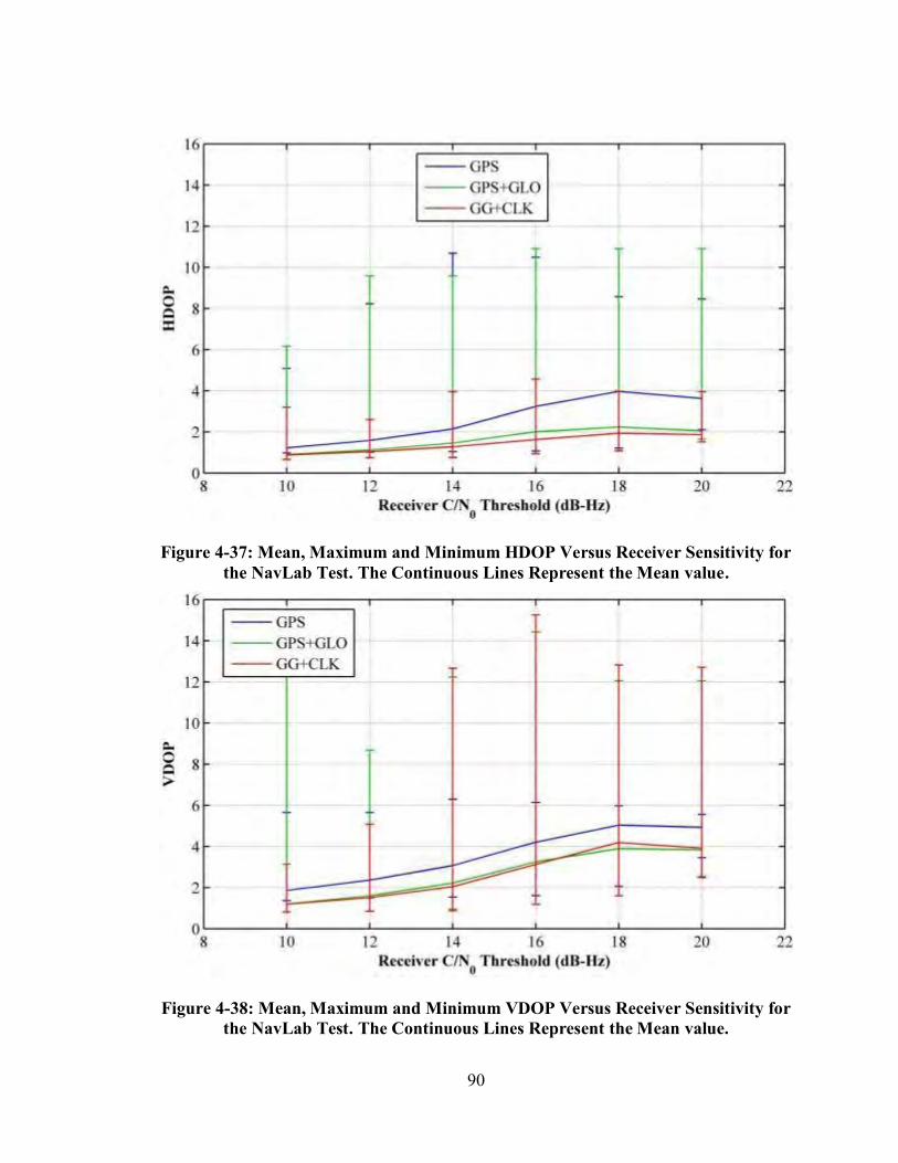
90
Figure 4-37: Mean, Maximum and Minimum HDOP Versus Receiver Sensitivity for the NavLab Test. The Continuous Lines Represent the Mean value.
Figure 4-38: Mean, Maximum and Minimum VDOP Versus Receiver Sensitivity for the NavLab Test. The Continuous Lines Represent the Mean value.

91
Finally, the RMS position errors are plotted in Figure 4-39 and Figure 4-40. Here there is
significant improvement in the horizontal position errors, particularly when the system
time offset is provided in addition to the GLONASS measurements.
Figure 4-39: Horizontal RMS Position Errors Versus Receiver Sensitivity for the NavLab Test
The results of the vertical position are somewhat mixed, particularly for higher C/N0
thresholds. For the 10 dB-Hz threshold there is, again, significant improvement (about
30 %) with the addition of GLONASS.

92
Figure 4-40: Vertical RMS Position Errors Versus Receiver Sensitivity for the NavLab Test
Increasing the coherent integration time in a digital matched filter (correlator) is the
optimal manner in which to improve receiver sensitivity (Kaplan & Hegarty 2006).
Recall from Equation (4.2), the signal to noise ratio (SNR) at the output of the correlator
is linearly proportional to the integration time, provided the local replica is perfectly
matched to the incoming signal. Increased coherent integration is a highly desirable
feature in a high sensitivity receiver. According to O’Driscoll et al (2008) and
Broumandan et al (2011), there are a number of challenges associated with increasing the
coherent integration time, such as tracking errors, data bit modulation and some stability
issues.

93
Figure 4-41 and Figure 4-42 show the horizontal and vertical RMS position errors versus
different coherent integration time. For this environment (NavLab test), by increasing the
coherent integration time, the RMS position errors decrease. There is significant
improvement in the horizontal and vertical position errors, particularly when the system
time offset is provided in addition to the GLONASS measurements. This is especially
noticeable when using a short coherent integration time.
Figure 4-41: Horizontal RMS Position Errors Versus Coherent Integration Time for the NavLab Test

94
Figure 4-42: Vertical RMS Position Errors Versus Coherent Integration Time for the NavLab Test
The percentage of epochs for which a solution was computed versus coherent integration
time is shown in Figure 4-43. It can be seen that adding GLONASS to a high sensitivity
receiver resulted in a significant improvement, particularly when the receiver coherent
are around the 200ms. For example, for a receiver with a coherent integration time of
200 ms, the availability of GPS solutions is approximately 60 %. When GLONASS is
added this increases to 83 %. Providing the system time offset yields 92 % solution
availability in this case.

95
Figure 4-43: Percentage Availability of Position Solutions Versus Coherent
Integration Time for the NavLab Test
In conclusion, by using a reference/rover configuration to observe GNSS signals indoors,
it has been shown that the behaviour of the GPS and GLONASS L1 C/A signals are
broadly similar in these environments. With the two test scenarios it appears that the
availability and accuracy benefits of adding GLONASS to high sensitivity receivers
become more significant the more challenging the environment. For moderate multipath
or open sky environments, the HS-GPS receiver performs sufficiently well for many
applications. For harsher environments (C/N0 of the order of 10 dB-Hz), improvements in
accuracy and availability of 30 % were observed when GLONASS capability was added.
The availability of an estimate of the GPS/GLONASS time offset can make a significant
difference in the availability and accuracy of solutions in scenarios with limited numbers
of satellites. The dynamic test results and analysis will be discussed in the next chapter.

96
Chapter Five: Dynamic Test Results and Analysis
5.1 Chapter Overview
This chapter explains and presents the relevant information pertaining to the field test and
results of the vehicular kinematic data collected in a North American urban canyon. The
analysis considers measurement availability, navigation solution availability, residual
analysis and position domain results.
5.2 Dynamic Test
The urban canyon environment is one in which the issue of signal availability is
particularly important. Tall buildings not only block signals entirely but act as strong
specular reflectors that induce large multipath effects and tracking of echo-only signals.
Even if sufficient satellites are visible, the geometric dilution of precision can often be
large, leading to large errors in position. In total, four kinematic tests were performed in
downtown Calgary. A NovAtel’s UIMU-LCI GPS/INS system was used to provide
reference trajectories of high accuracy. The IMU data was processed using the Inertial
Explorer™, which provided very accurate reference trajectories even when GPS
observations were not available for short periods of time. Not all tests were successful in
terms of obtaining precise reference navigation data. The longest data set results will be
presented in this chapter. Other test results were published by O’Driscoll et al (2010).
Following an overview of the signal and navigation processing strategies employed, a
description of the field test is provided. A data analysis consisting of navigation solution
availability, residual analysis and position domain results is presented.

97
5.3 Methodology
GSNRx™ was used to process the GPS/GLONASS data in standard and assisted high
sensitivity modes and to assess performance. The standard and HS receiver architecture
were discussed in detail in Chapter Three; therefore, they are not reviewed here.
5.4 Test Setup and Description
To test the relative performance of the various processing strategies a test was conducted
in downtown Calgary as described above. Data was collected using a National
Instruments PXI-5661 RF down converter and digitizer (National Instruments 2009) and
one NovAtel GPS702-GG model antenna. A nearby reference station, with a clear view
of the sky, located on the roof of the CCIT building at the University of Calgary, used a
NovAtel OEM4 in parallel to collect reference data. Figure 5-1 shows the experimental
setup for this scenario.
Raw measurements were logged at a 1s interval. The digitized data was post-processed in
two modes (standard and assisted HS GNSS) using GSNRx™. The parameters used in
the GSNRx™ are given in Table 5-1.
The trajectory followed is shown in Figure 5-2. The test trajectory included travel in the
downtown core of Calgary, specifically between 5 Ave and 6 Ave SW. The starting point
was at the intersection of 9 Ave SW and 11 Street SW. The experiment loop was
repeated six times over the course of 1h20m. A static period of approximately three
minutes was used to initialize the assisted HS GNSS processing at the beginning of the
experiment. During this period the vehicle had a mostly clear view of the sky. This static
initialization was followed by two loops. This process was repeated three times.

98
(a) Test Car
(b) Battery Setup (c) Experimental Setup Inside Test Car
Figure 5-1: Experimental Setup for Downtown Calgary Vehicular Test.
Table 5-1: Processing Parameters Used in GSNRx™
Parameter Standard HS-GNSS
TCoh 20 ms 100 ms
Code Range 1 Chip 900 m
Range Rate - 5 m/s
Code Range Spacing 0.5 Chip 60 m
Range Rate Spacing - 0.1 m/s

99
Figure 5-2: Test Trajectory Encompassing 5th and 6th Ave SW (1h20m Travel Time) (Google Maps 2011)
The majority of the test was travelled in an East-West direction, with significant signal
masking to the North and South. Masking angles exceeded 75 degrees. Figure 5-3 shows
a typical view during the test.
Figure 5-3: Typical View from Vehicle during the City Core Test

100
5.5 Experimental Results & Analysis
This section shows the results obtained using GSNRx™ in standard and high sensitivity
modes for the urban canyon test described above. The section includes results from the
combined GPS and GLONASS processing in terms of solution availability, the number
of satellites used in each solution, the DOP associated with each solution and the
statistics of solution residuals. Epoch-by-epoch least-squares and Kalman filter
estimation approaches are used for navigation solution results.
5.5.1 Measurements Availability
A sky plot of the satellites visible above a 5-degree elevation mask at the initialization
location is shown in Figure 5-4. A total of 11 GPS and 10 GLONASS satellites were
present. Nevertheless, two satellites were blocked from view, namely GLONASS SVs 11
and 18. As a result these SVs were not available for processing in the assisted HS GNSS
mode.
5.5.2 Standard Receiver Processing Results
Standard GSNRxTM was used to process the data in standard mode. This section includes
results from the combined GPS and GLONASS processing in terms of C/N0, least-
squares residual analysis, position solution availability and DOP. All least-squares
navigation solution results presented in this section were obtained in single point mode
using the PLAN Group C3NavG2™ software, which uses both code and Doppler
measurements and an unconstrained epoch-by-epoch solution approach. The
measurements out of GSNRx™ are not corrected for the effect of the atmosphere.

101
However C3NavG2™ applies a standard tropospheric correction to the measurements.
No corrections are made to the single frequency measurements for the effect of the
ionosphere, which is still low at this time. The Kalman filter navigation solution results
are presented at the end of this section.
Figure 5-4: GPS and GLONASS Satellite Availability at Start of the Downtown Test
The number of satellites tracked with GSNRx™ in standard mode is shown in Figure 5-5.
The effect of fading and multipath is observed in the subsequent figures. At the beginning
of the experiment, during which the receiver had a clear view of the sky, the receiver
tracked 11 GPS and 8 GLONASS satellites. Otherwise, in the city core, the number of
satellites varied due to the shadowing effect of large buildings, which resulted in poor
position estimation. The variation in the number of satellites tracked indicates the
frequency of loss of signal.

102
Figure 5-5: Number of Satellites Tracked with GSNRxTM in Standard Mode – Downtown Test
5.5.2.1 Carrier-to-Noise Density Ratio
Figure 5-6 and Figure 5-7 show the measured C/N0 at the antenna for GPS and
GLONASS satellites, respectively. Clearly this environment is considerably more
challenging due to fading and multipath. By starting the experiment with a largely clear
view of the sky most signals were observed with C/N0 values in the range of 40 to 50 dB-
Hz. In the downtown core the signals were affected by shadowing and multipath and the
received signals exhibited C/N0 values which varied between 5 and 40 dB-Hz. The
signals from GPS PRN 18 and GLONASS PRN 1 were less affected by multipath. These
satellites were at a reasonably high elevation.

103
Figure 5-6: Carrier-to-Noise Density Ratio of GPS Signals Received - Downtown Test
Figure 5-7: Carrier-to-Noise Density Ratio of GLONASS Signals Received - Downtown Test

104
As it can be seen from the above figures, the estimated C/N0 values are very similar for
both GPS and GLONASS. The received C/N0 values during the first three minutes of the
experiment are relatively high for both GPS and GLONASS because the receiver has a
relatively clear view of the sky. For the same reason this conclusion is applicable during
the period from about 1800 s to 2300 s, from 3300 s to 3800 s and finally from 4300 s till
the end of the experiment. These time periods include movement in and out from heavily
shaded areas, in addition to three minutes in static mode. On the other hand, the measured
C/N0 values of GPS and GLONASS satellites are highly varying the rest of the time
inside the city core as mentioned earlier.
5.5.2.2 Residual Analysis
To investigate the quality of the measurements, the residuals from the least-squares
solutions are studied as mentioned in Chapter Three. The residuals of these solutions
provide a measure of some of the unmodelled effects left in the measurements. The GPS
and GLONASS residuals are calculated using C3NAVG2TM. The measurements are
rejected if the standardized residual value exceeds 3.28 (MacGougan 2003). Only those
epochs for which redundant solutions are computed are considered here, since non-
redundant solutions lead to residuals with values of zero.
Figure 5-8 and Figure 5-9 show the histograms of the residuals from GPS and GLONASS
standard processing strategies. The summary statistics are shown in Table 5-2. The
results presented are limited to those epochs during which the vehicle was in the
downtown portion of the test. In total, 1703 GPS residual samples and 1051 GLONASS
samples are available for residual analysis. The maximum residual value is 10.6 m for
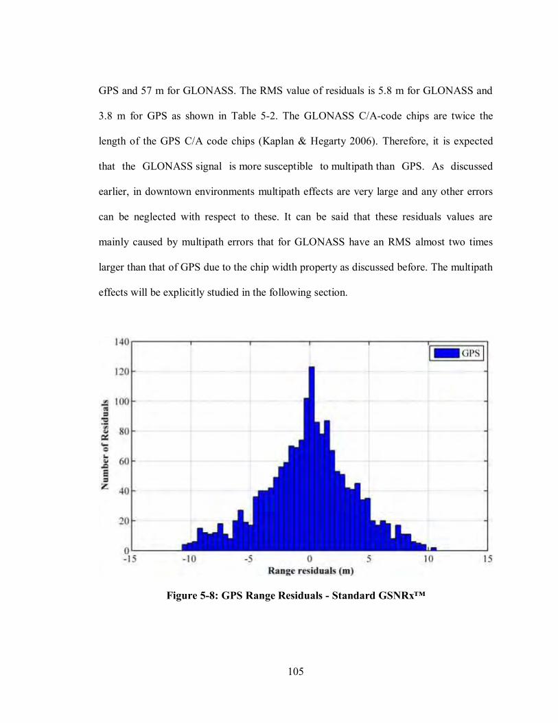
105
GPS and 57 m for GLONASS. The RMS value of residuals is 5.8 m for GLONASS and
3.8 m for GPS as shown in Table 5-2. The GLONASS C/A-code chips are twice the
length of the GPS C/A code chips (Kaplan & Hegarty 2006). Therefore, it is expected
that the GLONASS signal is more susceptible to multipath than GPS. As discussed
earlier, in downtown environments multipath effects are very large and any other errors
can be neglected with respect to these. It can be said that these residuals values are
mainly caused by multipath errors that for GLONASS have an RMS almost two times
larger than that of GPS due to the chip width property as discussed before. The multipath
effects will be explicitly studied in the following section.
Figure 5-8: GPS Range Residuals - Standard GSNRx™

106
Figure 5-9: GLONASS Range Residuals - Standard GSNRx™
Table 5-2: GPS-GLONASS Residuals Statistics - Standard GSNRx™
Parameter GPS GLONASS
Samples 1703 1051
Maximum (m) 10.6 57.4
RMS (m) 3.8 5.8
To illustrate the effect of multipath and receiver noise on the range measurements, it has
to be clearly stated what the other errors are that affect these measurements. The
pseudorange observation equation of the ith satellite is given by
,i i i i i i i i
ion trop p m pP c dt dT d d (5.1)
where

107
ρi : is the geometric range between satellite and receiver antenna [m],
δ ρi : is the satellite position error (broadcast ephemeris) [m] ,
c : is the speed of light [m/s],
dti : is the satellite clock error with respect to GPS time [s],
dT : is the receiver clock error with respect to GPS time [s],
dion : is the ionospheric error [m],
dtrop : is the tropospheric error [m],
,ip m : is the code multipath [m], and
ip : are the other code errors (considered to be stochastic) [m].
The satellite position errors and clock error are neglected due to an accurate clock
oscillator installed on the satellite. The ionospheric error is also neglected but is small at
this time as stated earlier. To eliminate the receiver clock error, the estimated clock error
from GSNRxTM are post processed to generate a model of the receiver clock drift error
behaviour and this model is then used to account for the receiver clock drift error. The
remaining errors will be mostly multipath and noise. The positions from the precise
GPS/INS reference trajectory are used to calculate the GPS/INS pseudoranges between
the satellites and the receiver. These pseudoranges are used to calculate the errors now
defined as the difference between GPS/INS derived pseudoranges and GPS and
GLONASS measured pseudoranges. Figure 5-10 and Figure 5-11 show the histograms of
these errors after eliminating the receiver clock drift error. Table 5-3 shows the GPS-
GLONASS statistics from Figure 5-10 and Figure 5-11.

108
Figure 5-10: GPS Pseudorange Errors Derived from Reference GPS/INS Trajectory - Standard GSNRxTM, Clock Drift Error Removed
Figure 5-11: GLONASS Pseudorange Errors Derived from Reference GPS/INS Trajectory - Standard GSNRxTM, Clock Drift Error Removed

109
Table 5-3: GPS-GLONASS Statistical Representation of Pseudorange Errors Derived from Reference GPS/INS Trajectory - Standard GSNRxTM
Parameter GPS GLONASS
Minimum (m) -10.7 -14.2
Maximum (m) 10.3 57.4
RMS (m) 2.3 4.7
As shown is Table 5-3, the RMS value of the GLONASS errors is larger than the RMS
value of the GPS errors. By comparing the RMS values of GPS and GLONASS in
Table 5-2 and Table 5-3, it is clear that the dominant errors are due to multipath and noise
effects in the urban canyon environment. As discussed before, the GLONASS signal is
slightly more affected by multipath than GPS.
Figure 5-12 and Figure 5-13 show the histograms of the range rate residuals of GPS and
GLONASS derived from C3NavG2™. Table 5-4 shows statistics relating to Figure 5-12
and Figure 5-13. It has already been mentioned that GPS uses a CDMA technique, while
GLONASS uses FDMA. The FDMA technique allows a better resistance to intra-system
interferences than CDMA (Rappaport 1996). The RMS values of the GPS and
GLONASS range rate residuals are almost the same.

110
Figure 5-12: GPS Range Rate Residuals for the Downtown Test - Standard GSNRxTM
Figure 5-13: GLONASS Range Rate Residuals for the Downtown Test - Standard GSNRxTM

111
Table 5-4: GPS-GLONASS Range Rate Residual Statistics (Downtown, Standard GSNRx™)
Parameter GPS GLONASS
Minimum (m/s) -0.14 -0.11
Maximum (m/s) 0.11 0.10
RMS (m/s) 0.02 0.02
5.5.2.3 Position Accuracy, Solution Availability and Dilution of Precision
A position solution was calculated using least-squares and Kalman filter estimation
techniques. A single-point epoch-by-epoch least-squares solution was computed at a 1 Hz
rate. If there were insufficient satellites in view at a given epoch or the solution failed to
converge in 10 iterations, no solution was computed. In this section, the analysis focuses
on position accuracy, DOP and the percentage of epochs during the downtown portion of
the test for which a solution was computed.
Figure 5-14 and Figure 5-15 show the percentage of solutions computed for various
navigation processing strategies as a function of HDOP and VDOP thresholds,
respectively. As shown in the figures, the Kalman filter solutions using a combination of
GPS and GLONASS yielded solutions with a HDOP of less than 6 85 % of the time. For
larger DOP thresholds it is clear that there is a 10% difference between GPS-only
processing and GPS/GLONASS processing. The biggest differences are caused by the
processing strategies employed. For this test and the particular geometry of the satellites
in view during the test, GPS/GLONASS processing does yield a noticeable improvement
with lower VDOP thresholds. The solution availability for the height fixed case when

112
HDOP is lower than 5 is 53 % for the combined GPS/GLONASS solution, as compared
to 47 % for the non-height fixed solutions.
Figure 5-14: Availability of Position Solutions Versus HDOP (Downtown, Standard GSNRx™)
Figure 5-15: Availability of Position Solutions Versus VDOP (Downtown, Standard GSNRx™)

113
The final stage of the analysis of standard processing techniques is a comparison of the
position accuracy computed using different navigation processing strategies (least-
squares and Kalman filter estimation techniques). The GPS/INS reference trajectory was
used for this purpose and is shown in black in the following figures. The following
section compares the navigation results of the least-squares and Kalman filter estimation
approaches.
5.5.2.3.1 Least-squares estimation approach
Figure 5-16 shows the trajectories obtained using standard wide correlator processing
with no height fixing. The maximum HDOP used in the figure is 5. There are very large
position errors for the standard receiver due to the measurement of cross-correlation and
echo-only signals. The 2D position errors reach 425 m at one point. The resulting
geometry is poor.
The solution availability concerning horizontal positions with good geometry, HDOP
lower than 5, and with fault exclusion enabled is 48% for the standard processing when
using GPS and GPS/GLONASS observations. The addition of GLONASS does not result
in a noticeable improvement in terms of availability in this case. The time series analysis
of the position errors are in the following section.

114
Figure 5-16: Test Trajectory (Least-Squares, No Height Fixing, Standard GSNRxTM) - Downtown Test
Figure 5-17 shows a time series analysis of the horizontal positioning solutions with non-
height fixing by using a standard GSNRx™ during the Downtown Test. The accuracy
and availability performance improvements when adding GLONASS are insignificant.
Table 5-5 shows the time series statistics of Figure 5-17. In fact, it appears that the
addition of GLONASS occasionally leads to biases in the navigation solutions for DOP
values near 5. It was shown previously that the urban canyon environment is severe in
terms of the measurement errors induced by multipath, echo-only signal tracking, and
signal cross-correlation effects. For conventional GPS/GLONASS and HS
GPS/GLONASS to be useful in such an environment, errors due to cross-correlation
tracking of echo-only signals should be removed or deweighted in the estimator used.

115
Figure 5-17: Time Series Analysis of Horizontal Position Solutions (Least-Squares, No Height Fixing, Standard GSNRxTM) - Downtown Test

116
Table 5-5: Time Series Statistics of Horizontal Position Solutions (Least-Squares, No Height Fixing, Standard GSNRxTM) - Downtown Test
Parameter 2D Position Errors (m) HDOP GPS GPS + GLONASS GPS GPS + GLONASS
Minimum 0.9 0.6 0.9 0.8
Maximum 422 425 5 4.9
RMS 79 75 1.9 1.9
As seen from the figure above, there is a 35s duration where the position error is
approximately 400 m (GPS time 412945 - 412980 s). Four GPS and two GLONASS
satellites are available during these epochs and provide an HDOP of 3.9. At GPS time
412950 s, the range residuals of the four GPS satellites are -0.33 m, 2.77 m, -0.13 m and -
2.3 m (PRNs 3, 18, 19 and 22, respectively). The residuals of the two GLONASS
satellites (PRN 1 and 17) are -4.4 m and 4.4 m. Thus, since the epoch had a redundancy
of 1 (six observations and five parameters), the ability to perform residual testing is
compromised (O’Keefe et al 2011). Additionally, given that the redundancy of the
GLONASS satellite clock time parameter is 1 (two GLONASS satellites), the GPS
residuals are not of the same magnitude because the GLONASS observations are
providing observability in position domain.
As shown in Appendix A, the standardized range residuals of the four GPS SVs, which
are the square root of the a posteriori variance factor and equal to the length of the
residual vector, are -1.44, 1.44, -1.44 and -1.44 (PRNs 3, 18, 19 and 22, respectively).
The standardized range residuals of the two GLONASS satellites (PRN 1 and 17) are -
1.44 and 1.44. The absolute value of the standardized residuals from all the satellites is

117
the same. Thus, while the global test can be used to determine if an outlier is present,
least squares residual testing to isolate the outlier at this particular epoch will clearly fail.
This means that if observations at this particular epoch contain significant multipath, it
will be undetectable even though the geometry is still reasonable.
In kinematic testing the height is often well known, and the height during the test
trajectory varied by less than 15 m, thus a height fix will be used to improve the ability to
detect measurement faults and improve horizontal position accuracy. Dilution of
precision, DOP, will be indicated for each solution computed to assess the influence of
solution geometry. The height was obtained by averaging the height values output by the
GPS/INS system during the first static three minutes of the experiment.
Figure 5-18 shows a time series analysis of horizontal position solutions by using
standard GSNRxTM in the downtown Calgary test. The addition of GLONASS improves
the position accuracy and DOP. Table 5-6 shows the GPS-GLONASS statistics from
Figure 5-18. RMS horizontal errors of 78 and 64 m are typical for this testing case when
using the GPS and GPS/GLONASS measurements at HDOP lowers than 5. At some
times in the experiment, the resulting geometry is very poor and an 880 m horizontal
position error still occurs.

118
Figure 5-18: Time Series Analysis of Horizontal Position Solutions (Least-Squares, Height Fixing, Standard GSNRxTM) - Downtown Test

119
Table 5-6: Time Series Statistics of Horizontal Position Solutions (Least-Squares, Height Fixing, Standard GSNRxTM) - Downtown Test
Parameter 2D Position Errors (m) HDOP
GPS GPS + GLONASS GPS GPS + GLONASS
Minimum 0.5 0.3 1.1 0.8
Maximum 880 880 4.9 4.9
RMS 78 61 2.3 2.1
5.5.2.3.2 Kalman Filter Approach
Kalman filtering is a classical estimation algorithm using both measurements and
dynamics. The Kalman filter estimation technique was discussed in Chapter Three. The
Kalman filter implemented in the GSNRxTM is used to get the following KF results. The
system model uses a random walk velocity model (Brown & Hwang 1992). The
estimated C/N0 is used to weight the measurements. A summary of the parameters used
to adjust the Kalman filter:
pseudorange standard deviation at zenith (m) : 10.0
Doppler standard deviation at zenith (Hz) : 2
phase standard deviation at zenith (cycles) : 0.1
east velocity spectral density (m/s/root-Hz) : 10.0
north velocity spectral density (m/s/root-Hz) : 10.0
vertical velocity spectral density (m/s/root-Hz) : 0.5

120
Figure 5-19 shows the trajectory by using the Kalman filter to calculate the navigation
solutions. By comparing the results of least-squares and Kalman filter estimation
techniques, the filtering in the Kalman filter solution improves the position accuracy.
Figure 5-19: Test Trajectory (Kalman Filter, Standard GSNRxTM) - Downtown Test
Figure 5-20 shows the time series analysis of the horizontal position errors processed
using the Kalman filter approach. Table 5-7 shows the statistical representation of
Figure 5-20. A marked improvement in the availability and position errors can be
observed when the Kalman filter is used, as expected. The addition of GLONASS in this
case improves solution availability. By adding GLONASS a small improvement in
position accuracy and DOP was noticed. RMS horizontal errors of 18 and 17 m are
obtained for this case when using GPS and GPS/GLONASS measurements, respectively.
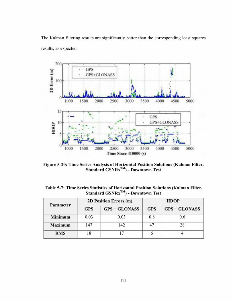
121
The Kalman filtering results are significantly better than the corresponding least squares
results, as expected.
Figure 5-20: Time Series Analysis of Horizontal Position Solutions (Kalman Filter, Standard GSNRxTM) - Downtown Test
Table 5-7: Time Series Statistics of Horizontal Position Solutions (Kalman Filter, Standard GSNRxTM) - Downtown Test
Parameter 2D Position Errors (m) HDOP
GPS GPS + GLONASS GPS GPS + GLONASS
Minimum 0.03 0.03 0.8 0.6
Maximum 147 142 47 28
RMS 18 17 6 4

122
5.5.3 High Sensitivity Receiver Processing Results
HS-GSNRxTM was used to process the data in high sensitivity mode. This section
includes results from the combined GPS and GLONASS systems in terms of C/N0
density ratio, least-squares residual analysis and position solution, solution availability
and DOP. The least squares and Kalman filter estimation techniques were used to
produce navigation solutions.
The number of satellites tracked by using the HS-GSNRx™ for the downtown Calgary
test is shown in Figure 5-21. The receiver was able to track 11 GPS and 8 GLONASS
satellites during the test. The HS receiver clearly obtains more measurements than the
standard receivers, although all receivers tracked a sufficient number of satellites to
obtain a full navigation solution during most of the test. By combining GLONASS with
GPS, measurement availability was increased which led to improvement in position
accuracy, solution availability and DOP. There was less variation in the number of
satellites tracked by the HS receiver than the standard receiver, indicating less frequent
loss of signal lock.

123
Figure 5-21: Number of Satellites Tracked with the HS-GSNRxTM
5.5.3.1 Carrier-to-Noise Density Ratio
Figure 5-22 and Figure 5-23 show the output C/N0 values for GPS and GLONASS
satellites, respectively, processed by the HS-GSNRxTM. The C/N0 values are less noisy
than those obtained in standard processing mode. The levels and the trends observed in
the C/N0 values are very similar between GPS and GLONASS. Again, the fading
environment appears very similar in each case. It is evident that the low elevation
satellites were affected more by multipath than the satellites at high elevation. As an
example, GPS PRN 18 and GLONASS PRN 1 have less multipath effects than the lower
satellites. The C/N0 values vary rapidly in the downtown core due to the shadowing
effects of large building, which results in multipath and echo-only signals.

124
Figure 5-22: Carrier-to-Noise Density Ratio of GPS Signals (Downtown Test, HS-GSNRx™)
Figure 5-23: Carrier-to-Noise Density Ratio of GLONASS Signals (Downtown Test, HS-GSNRx™)

125
5.5.3.2 Residual Analysis
Figure 5-24 and Figure 5-25 show the histograms of the range residuals from the high
sensitivity processing of GPS and GLONASS.
Table 5-8 show the statistics pertaining to Figure 5-24 and Figure 5-25, respectively.
Clearly the assisted HS-GSNRx™ has a greater availability of redundant solutions
compared to the standalone receiver, which is to be expected. The assisted HS receiver
residuals have a slightly lower RMS as compared to a standard receiver, indicating that
the navigation solution absorbs more of the measurement errors in this case. These results
indicate also that the GLONASS measurements are more affected by multipath than GPS
measurements as discussed earlier.
Figure 5-24: GPS Pseudorange Residuals (Downtown Test, HS-GSNRx™)

126
Figure 5-25: GLONASS Peudorange Residuals (Downtown Test, HS-GSNRx™)
Table 5-8: GPS-GLONASS Pseudorange Statistics (Downtown Test, HS-GSNRx™)
Parameter GPS GLONASS
Minimum (m) -11 -13.7
Maximum (m) 10.9 14.6
RMS (m) 3.7 5.4
Figure 4-27 and Figure 5-27 show the histograms of the pseudorange errors derived from
reference GPS/INS trajectory of GPS and GLONASS after eliminating the receiver clock
drift error. Table 5-9 shows statistics pertaining to Figure 4-27 and Figure 5-27. Similar
to the standard processing techniques, the GLONASS measurements are more noisy then
the GPS measurements. The RMS value of the GPS errors is 3.2 m and the RMS value of
the GLONASS errors is 5.3 m.

127
Figure 5-26: GPS Pseudorange Errors Derived from Reference GPS/INS Trajectory - High Sensitivity GSNRxTM, Clock Drift Error Removed
Figure 5-27: GLONASS Pseudorange Errors Derived from Reference GPS/INS Trajectory - High Sensitivity GSNRxTM, Clock Drift Error Removed

128
Table 5-9: GPS-GLONASS Statistical Representation of Pseudorange Errors Derived from Reference GPS/INS Trajectory - High Sensitivity GSNRxTM
Parameter GPS GLONASS
Minimum (m) -10.9 -13.7
Maximum (m) 10.9 13.9
RMS (m) 3.2 5.3
The number of residuals available is different between standard and HS solutions, as the
latter produce more measurements and more redundant solutions, hence more residuals.
The processing strategy, therefore, has a significant impact on the availability of
redundant solutions. Figure 5-28 and Figure 5-29 show the histograms of the range rate
residuals of GPS and GLONASS derived from C3NavG2™. Table 5-10 shows the
statistics relating to Figure 5-28 and Figure 5-29. The RMS values of the GPS and
GLONASS range rate residuals are almost the same around 0.03 m/s.
Figure 5-28: GPS Range Rate Residuals - High Sensitivity GSNRxTM

129
Figure 5-29: GLONASS Range Rate Residuals - High Sensitivity GSNRxTM
Table 5-10: GPS-GLONASS Range Rate Residual Statistics - High Sensitivity GSNRxTM
Parameter GPS GLONASS
Minimum (m/s) -0.19 -0.16
Maximum (m/s) 0.18 0.18
RMS (m/s) 0.04 0.03
5.5.3.3 Position Accuracy, Solution Availability and Dilution of Precision
Least-squares and Kalman filter estimation approaches were used to process the
navigation solution of the high sensitivity receiver. In this section, the analysis focuses on
position accuracy, DOP and the percentage of epochs during the downtown portion of the
test for which a solution was computed.

130
Figure 5-30 and Figure 5-31 show the percentage of solutions computed using least-
squares and Kalman filter approaches for navigation solutions as a function of HDOP and
VDOP thresholds, respectively. As shown in these figures, the biggest differences are
caused by the processing strategies employed. The advantages of HS processing are clear,
at least in terms of solution availability. GPS/GLONASS processing does yield a
noticeable improvement in the lower thresholds of HDOP and VDOP. This is noticeable
in Figure 5-30 and Figure 5-31. When a Kalman filter approach is used, the solution
availability is 100 %. The reason is the design of the Kalman filter which can obtain a
navigation solution from at least one measurement.
Figure 5-30: Availability of Position Solutions Versus HDOP Threshold (Downtown, HS-GSNRx™)

131
Figure 5-31: Availability of Position Solutions Versus VDOP Threshold (Downtown, HS-GSNRx™)
5.5.3.3.1 Least-squares approach
Figure 5-32 shows the trajectories obtained from the HS receiver. In this case the position
solutions are significantly less noisy than in previous cases. In addition, more solutions
are available. The quality of the GPS only and GPS/GLONASS results are broadly
similar. The time series analysis of the position accuracy and DOP are discussed in more
detail in the following sections.

132
Figure 5-32: Test Trajectory (Least Squares, No Height Fixing, HS-GSNRxTM) - Downtown Test
Figure 5-33 shows the horizontal error time series analysis of the assisted high sensitivity
processing techniques using a least-squares estimation technique with no height fixing.
Table 5-11 shows the related statistics. In this case, the addition of GLONASS results in
an improvement of availability. The RMS values shown in Table 5-11 suggest that
accuracy is not significantly improved by the addition of GLONASS signals in this case.
There is little improvement in DOP as shown in Table 5-11. RMS horizontal errors of 86
and 76 m are typical for this testing case when using the GPS and GPS/GLONASS
measurements with an HDOP of 5 or less.
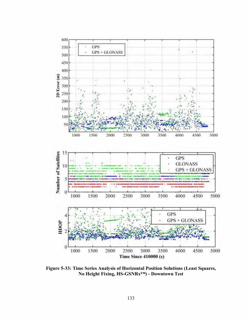
133
Figure 5-33: Time Series Analysis of Horizontal Position Solutions (Least Squares, No Height Fixing, HS-GSNRx™) - Downtown Test

134
Table 5-11: Horizontal Position Solution Statistics (Least Squares, No Height Fixing, HS-GSNRx™) - Downtown Test
Parameter 2D Position Errors (m) HDOP
GPS GPS + GLONASS GPS GPS + GLONASS
Minimum 0.8 0.7 0.9 0.8
Maximum 335 627 4.8 4.9
RMS 86 76 2.2 1.7
The analysis was repeated using a least-squares estimation technique with height fixing.
The height was obtained as described previously. Figure 5-34 shows a time series
horizontal position solution analysis by using a least-squares estimation technique with
height fixing. Table 5-12 shows the statistics. The positions are less noisy then previous
cases, though the addition of GLONASS does lead to some significant outliers. Position
availability is higher than that of the standard processing technique. Similar to the least-
squares estimation technique with no height fixing case, the addition of GLONASS again
appears to introduce an error in the solution during some epochs. RMS horizontal errors
of 96 and 70 m are typical for this testing case when using the GPS and GPS/GLONASS
measurements with a maximum HDOP of 5. The height fixing solution is slightly better
in terms of position availability and accuracy. RMS horizontal errors of 76 and 70 m are
obtained for this testing case when using the GPS/GLONASS measurements with non-
height and height fixing, respectively, with a maximum HDOP of 5.

135
Figure 5-34: Time Series Analysis of Horizontal Position Solutions (Least Squares, Height Fixing, HS-GSNRx™) - Downtown Test

136
Table 5-12: Horizontal Position Solution Statistics (Least Squares, Height Fixing, HS- GSNRx™) - Downtown Test
Parameter 2D Position Errors (m) HDOP
GPS GPS + GLONASS GPS GPS + GLONASS
Minimum 0.8 0.8 1 0.8
Maximum 585 371 4.9 4.7
RMS 96 70 2 1.6
5.5.3.3.2 Kalman filter approach
Figure 5-35 shows the trajectory when using the Kalman filter described earlier to
calculate the navigation solution. As shown in the figure, the results show that the
Kalman filter algorithm is effective most of the time with the exception of rare events
such as when making sharp turns. This is caused by heavy constraints in the filter which
result in over-shooting effects.
Figure 5-35: Test Trajectory (Kalman Filter, HS-GSNRx™) - Downtown Test

137
Figure 5-36 shows the time series analysis of the horizontal position errors processed
using the Kalman filter approach. Table 5-13 shows the related statistics. The addition of
GLONASS in this case results in significant improvements in solution availability,
position accuracy and DOP. RMS horizontal errors of 18 and 14 m are typical for this
testing case when using the GPS and GPS/GLONASS measurements and a maximum
HDOP of 5.
Figure 5-36: Time Series Analysis of Horizontal Position Solutions (Kalman Filter, HS- GSNRx™) - Downtown Test
Table 5-13: Time Series Statistics of Horizontal Position Solutions (Kalman Filter, HS- GSNRx™) - Downtown Test
Parameter 2D Position Errors (m) HDOP
GPS GPS + GLONASS GPS GPS + GLONASS
Minimum 0.06 0.07 0.7 0.5
Maximum 130 92 1 1
RMS 18 14 0.9 0.7

138
Chapter Six: Conclusions and Recommendations
6.1 Chapter Outline
This chapter summarizes the contributions of this thesis regarding the benefits of
combined GPS/GLONASS processing using high sensitivity receivers. The conclusions
of this research are presented and possible future work in this field of research is
recommended.
6.2 Conclusions
Data has been collected in static and dynamic test scenarios. Static data was collected in
two scenarios: A typical North American wooden house and an engineering laboratory
inside the Calgary Center for Innovative Technologies (CCIT) building of the University
of Calgary. In the two static test scenarios, the reference/rover receiver configuration was
used to process indoor GPS/GLONASS L1 C/A signals. Using a reference/rover
configuration to observe GNSS signals indoors, it has been shown that the behaviour of
the GPS and GLONASS L1 C/A signals are broadly similar in these environments. For
the two test scenarios considered, it appears that the availability and accuracy benefits of
combined GLONASS and GPS processing become more significant as the environment
becomes more challenging from a signal acquisition and tracking point of view. For
moderate multipath or open sky environments, the HS-GPS receiver performs well
(O’Driscoll et al 2010). For harsher environments (C/N0 of 10 dB-Hz), improvements in
accuracy and availability of 30 % were observed when GLONASS capability was added
as shown in Chapter Four. In static scenarios with a limited number of satellites, the

139
availability of a GPS/GLONASS time offset estimate can make a significant difference in
the availability and accuracy of solutions.
Vehicular kinematic data was collected in urban canyons using the PLAN Group
software receiver GSNRx™. The results show that high sensitivity processing is a very
effective means of improving navigation performance in urban canyon environments.
There are two primary advantages to HS processing in this case. The first advantage over
the standard tracking technique is the open-loop nature of HS processing. The time-
varying nature of the multipath channel causes significant variation in signal level. This
variation can cause traditional tracking loops to lose lock. In fact, the poor performance
of the standard wide correlator strategy in the above analysis can be explained by the fact
that the receiver was unable to maintain lock on the satellites in view. Hence no
measurements were generated and no solutions computed.
The second advantage of assisted HS processing relates to the longer coherent integration
time and the vehicle dynamics. As the receiver antenna moves through the multipath
environment a different Doppler shift is observed in signals coming from different
directions. Thus the line of sight and multipath components become separated in
frequency. A longer coherent integration time increases the frequency resolution of the
correlator output. Thus if the line of sight is present and the coherent integration time is
long relative to the inverse of the Doppler difference between the line of sight and
reflected signals, individual peaks become visible in the grid of correlators. This effect
can significantly reduce the impact of multipath on the measurements.
The addition of GLONASS capability can significantly improve the position solution
availability in urban canyons. Based on this research, in urban multipath environments

140
the greatest benefits are seen when combining GPS/GLONASS measurements in the HS
GNSS processing strategy. In addition, the use of a Kalman filter estimation approach
significantly improves position accuracy.
6.3 Recommendations
The following are some of the recommendations for future work in this research area:
1. Advanced tracking architectures such as vector tracking and/or ultra-tight
integration with inertial sensors for tracking weaker signals should be developed
and tested.
2. Dual-frequency measurements should be employed, as almost all current
GLONASS satellites transmit civil signals at both L1 and L2. The frequency
diversity may lead to advantages.
3. Signals from other GNSS such as Galileo should be added when they become
available. This will increase the accuracy and reliability of the navigation
solution.
4. The position results shown in this thesis are based on relatively good initial
estimates of the trajectory. The use of positions obtained through an internal filter
should be tested to confirm that the same level of accuracy can be obtained.

141
Reference
Abbasiannik, S. (2009) Multichannel Dual Frequency GLONASS Software Receiver in Combination with GPS L1 C/A, UCGE Reports No. 20215, Department of Geomatics Engineering, University of Calgary. Bao, J., and Y. Tsui (2000) Fundamentals of Global Positioning System Receivers: a Software Approach, John Wiley & Sons, Inc. Brown, G., and P. Hwang (1992) Introduction to Random Signals and Applied Kalman Filtering, John Wiley & Sons, Inc. Cai, C. (2009) Precise Point Positioning Using Dual-Frequency GPS and GLONASS Measurements, UCGE Reports No. 20291, Department of Geomatics Engineering, University of Calgary. Defraigne, P., Q. Baire, and N. Guyennon (2007) "GLONASS and GPS PPP for Time and Frequency Transfer," In proceeding of Frequency Control Symposium, 2007 Joint with the 21st European Frequency and Time Forum. IEEE International, 29 May – 1 June 2007. Enge, P., R. Fan, A. Tiwari, A. Chou, W. Mann, A. Sahai, J. Stone, and B. Roy (2001) "Improving GPS Coverage and Continuity: Indoors and Downtown," In Proceedings of the Institute of Navigation ION GPS-2001, September 11-14, 2001, Salt Lake, Utah, pages 3067–3076 Gao, G. (2007) INS-Assisted High Sensitivity GPS Receivers for Degraded Signal Navigation, UCGE Reports No. 20252, Geomatics Engineering, University of Calgary. GLONASS ICD (2008) http://www.GLONASS-ianc.rsa.ru, last accessed 20 April, 2011. Google Maps (2011) http://maps.google.ca/, last accessed 21 June, 2011. GPS ICD (2010) http://www.gps.gov/technical/icwg/, last accessed 9 April, 2011. GPS World (2011) "GLONASS K-1 Launched, Now Being Tracked," GPS World, 28 Feb. 2011. Grewal, M., and A. Andrews (2001) Kalman filtering: Theory and Practical Using Matlab 2nd Edition, John Wiley & Sons, Inc.

142
Haddrell, T., and A. R. Pratt (2001) "Understanding the Indoor GPS Signal," In proceeding of ION GPS-2001, Sep 11-14, Salt Lake City, UT Kang, J., Y. LEE, and J. Park (2002) "Enhancement of Continuty and Accuracy by GPS/GLONASS Combination, and Software Development," Korean Journal of Geomatics, vol 2, no 1, pp. 65-73. Kaplan, E., and C. Hegarty (2006) Understanding GPS Principle and Applications 2nd Edition, Artech House, Inc. Karunanayake, D., M. E. Cannon, G. Lachapelle, and G. Cox (2004) "Evaluation of AGPS in Weak Signal Environments Using a Hardware Simulator," In proceeding of ION GNSS 2004, 21-24 September, Long Beach, CA, pp. 2416-2426. Kay, S. (1993) Fundamentals of Statistical Signal Processing: Estimation Theory, Upper Saddle River, Prentice-Hall, New Jersey, USA. Keong, J. (1999) Determining Heading and Pitch Using a Single Difference GPS/GLONASS Approach, UCGE Reports No. 20134, Department of Geomatics Engineering, University of Calgary. Lachapelle, G. (2009) GPS Theory and Applications. ENGO 625 Course Lecture Notes, Department of Geomatics Engineering, University of Calgary. Lin, T., C. O’Driscoll, and G. Lachapelle (2011) "Development of a Context-Aware Vector-Based High-Sensitivity GNSS Software Receiver " In proceeding of International Technical Meeting, 24-26 January, San Diego, USA. MacGougan, G. (2003) High Sensitivity GPS Performance Analysis in Degraded Signal Environments, UCGE Report No. 20176, Department of Geomatics Engineering, University of Calgary. Misra, P. N., R. I. Abbot, and E. M. Gaposchkin (1996) "Integrated Use of GPS and GLONASS: Transformation between WGS84 and PZ-go," In proceeding of ION GPS-96, September 1996, Kansas City, MO, pp. 345-402. Mitelman, A., P.-L. Normark, M. Reidevall, J. Thor, O. Grönqvist, and L. Magnusson (2006) "The Nordnav Indoor GNSS Reference Receiver," In proceeding of ION-GNSS 2006, September 26-29, Fort Worth, TX, USA. National Instruments (2009) "NI PXI-5661 Specifications," Product Sheet. NovAtel (2007) GPS+ Reference Manual Rev 0I. NovAtel Inc. (2011) "GPS 701GG and 702GG,” Product Sheet.

143
O'Driscoll, C., and D. Borio (2009) GNSS Receiver Design. ENGO 638 Course Lecture Notes, Department of Geomatics Engineering, University of Calgary. O’Driscoll, C., M. Tamazin, D. Borio, and G. Lachapelle (2010) "Investigation of the Benefits of Combined GPS/GLONASS for High Sensitivity Receiver," In proceeding of GNSS10, Portland, OR, 21-24 Sep, 12 pages, The Institute of Navigation. O’Keefe, K., G. Lachapelle, A. Fazio, and D. Bettinelli (2011) "Receiver autonomous integrity monitoring in urban vehicle navigation: The five satellite case," Submitted to Journal of Global Positioning Systems, June 2011. Parkinson, B., J. Spilker, P. Axelrad, and P. Enge (1996) Global Positioning System: Theory and Applications, American Instite of Aeronautics and Astronautics, Inc., Washington, USA. Petovello, M. (2009) Estimation for Navigation. ENGO 699.18 Course Lecture Notes, Department of Geomatics Engineering, University of Calgary. Petovello, M., and G. Lachapelle (2006) "Comparison of Vector-Based Software Receiver Implementations With Application to Ultra-Tight GPS/INS Integration," Proceedings of GNSS06, Session C4, 26-29 Sep, Forth Worth, The Institute of Navigation. Petovello, M. G., C. O'Driscoll, G. Lachapelle, D. Borio, and H. Murtaza (2008) "Architecture and Benefits of an Advanced GNSS Software Receiver," In proceeding of International Symposium on GPS/GNSS 2008, Tokyo, Tokyo, Japan. Rappaport, T. (1996) Wireless Communications: Principles & Practice, 2nd Edition, Prentice Hall, New Jersey. Ryan, S., S. Stephen, J.H. Keong, M.G. Petovello, G. Lachapelle and R. Hare (1998) “Combination of GPS and GLONASS for Hydrographic Applications Under Signal Masking,” In proceeding of 1998 Canadian Hydrographic Conference, Victoria, B.C., March 9-12. Roongpiboonsopita, D., and H. Karimia (2009) "A Multi-Constellations Satellite Selection Algorithm for Integrated Global Navigation Satellite Systems," Journal of Intelligent Transportation Systems, pp. 127- 142. Satyanarayana, S., D. Borio, and G. Lachapelle (2009) "GPS L1 Indoor Fading Characterization using Block Processing Techniques," In proceeding of ION GNSS 2009, 22-25 September, Savannah, GA.

144
Urlichich, Y., V. Subbotin, G. Stupak, V. Dvorkin, A. Povalyaev, and S. Karutin (2011) "Innovation: GLONASS Developing Strategies for the Future," In: GPS World, Edition April, 2011. Van Dierendonck, A. J. (1995) GPS Receivers, Global Positioning System: Theory and Applications, B. W. Parkinson and J. J. Spilker, Jr., American Institute of Aeronautics and Astronautics, Inc. Watson, J. (2005) High-Sensitivity GPS L1 Signal Analysis for Indoor Channel Modelling, UCGE Reports No. 20215, Department of Geomatics Engineering, University of Calgary. Welch, G., and Bishop, G. (2001) An Introduction to the Kalman Filter. Department of Computer Science, University of North Carolina. Yongjun, Z. and Zemin, W. (2002) “Analyses and Solutions of Errors on GPS/GLONASS Positioning” Geo-Spatial Information Science, Vol. 5, No. 2, Pages 6-12, June 01, 2002.

145
Appendix A Least-Squares GPS/GLONASS Testing Residuals with One Degree of
Freedom
This appendix derives the mathematical equivalence to show the problem of
GPS/GLONASS testing residuals with one degree of freedom when using single epoch
least squares for vehicle navigation at Calgary downtown.
The results shown at this appendix of particular data epoch occurs at GPS time 412950
and was collected by using GSNRx™ software receiver in core of Calgary downtown
which was discussed in Chapter Five. At this time, total of 11 GPS and 10 GLONASS
satellites were present, but only 4 GPS and 2 GLONASS satellites were being tracked
during this epoch and provide an HDOP of 3.9. The satellites elevations azimuths and
pseudorange are given in Table A.1.
Table A.1: GPS/GLONASS pseudorange observations
Satellite Elevation Azimuth Pseudorange (m)
GPS PRN 3 38.20 262.3 21796020.24
GPS PRN 18 74.90 70.5 20505590.04
GPS PRN 19 33.60 303.1 22535286.53
GPS PRN 22 68.80 260.9 20565456.95
GLONASS PRN 1 67.56 30.05 19505975.98
GLONASS PRN 17 56.02 290.69 20036912.26
The corresponding design matrix, with columns corresponding to latitude, longitude,
height and GPS and GLONASS clock offset for this epoch is
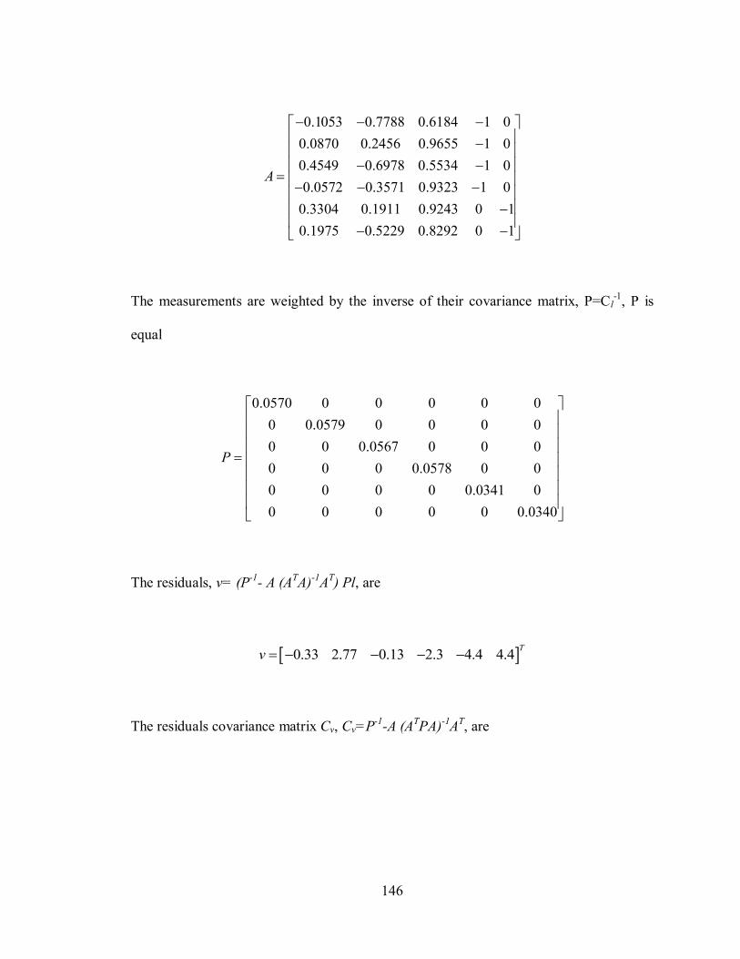
146
0.1053 0.7788 0.6184 1 00.0870 0.2456 0.9655 1 00.4549 0.6978 0.5534 1 00.0572 0.3571 0.9323 1 0
0.3304 0.1911 0.9243 0 10.1975 0.5229 0.8292 0 1
A
The measurements are weighted by the inverse of their covariance matrix, P=Cl-1, P is
equal
0.0570 0 0 0 0 00 0.0579 0 0 0 00 0 0.0567 0 0 00 0 0 0.0578 0 00 0 0 0 0.0341 00 0 0 0 0 0.0340
P
The residuals, v= (P-1- A (ATA)-1AT) Pl, are
0.33 2.77 0.13 2.3 4.4 4.4 Tv
The residuals covariance matrix Cv, Cv=P-1-A (ATPA)-1AT, are

147
0.0536 -0.4441 0.0223 0.3698 0.7064 -0.7078-0.4441 3.6771 -0.1848 -3.0615 -5.8482 5.86020.0223 -0.1848 0.0093 0.1539 0.2940 -0.29460.3698 -3.0615 0.1539 2.5489 4.8691 -4.87910.7064 -5.8482 0.2940 4.8691 9.3013 -9.3204-0.70
vC
78 5.8602 -0.2946 -4.8791 -9.3204 9.3395
The standardized range residuals, { }
i
v ii
vC
for i=1,2,…,n, of the 4 GPS and 2 GLONASS
satellites are
[ 1.4417 1.4417 1.4417 1.4417 1.4417 1.4417]Tv
Each one being equal to ± the square root of the sum of square of the residuals
2.0785 1.4417 . Here, a global test on the magnitude of this vector would clearly fail,
but isolating the bias would not be possible through evaluation of the standard residuals.


