
Understanding the Electronic
Structure of LiFePO4 and FePO4
A Thesis Submitted to the
College of Graduate Studies and Research
in Partial Fulfillment of the Requirements
for the degree of Master of Science
in the Department of Physics and Engineering Physics
University of Saskatchewan
Saskatoon
By
Adrian Hunt
c©Adrian Hunt, January 2007. All rights reserved.

Permission to Use
In presenting this thesis in partial fulfilment of the requirements for a Postgrad-
uate degree from the University of Saskatchewan, I agree that the Libraries of this
University may make it freely available for inspection. I further agree that permission
for copying of this thesis in any manner, in whole or in part, for scholarly purposes
may be granted by the professor or professors who supervised my thesis work or, in
their absence, by the Head of the Department or the Dean of the College in which
my thesis work was done. It is understood that any copying or publication or use of
this thesis or parts thereof for financial gain shall not be allowed without my written
permission. It is also understood that due recognition shall be given to me and to the
University of Saskatchewan in any scholarly use which may be made of any material
in my thesis.
Requests for permission to copy or to make other use of material in this thesis in
whole or part should be addressed to:
Head of the Department of Physics and Engineering Physics
116 Science Place
University of Saskatchewan
Saskatoon, Saskatchewan
Canada
S7N 5E2
i

Abstract
This thesis has detailed the extensive analysis of the XAS and RIXS spectra of
LiFePO4 and FePO4, with the primary focus on LiFePO4. One of the primary
motivations for this study was to understand the electronic structure of the two
compounds and, in particular, shed some light on the nature of electron correlation
within the samples. Two classes of band structure calculations have come to light.
One solution uses the Hubbard U parameter, and this solution exhibits a band gap of
about 4 eV. Other solutions that use standard DFT electron correlation functionals
yield band gaps between 0 and 1.0 eV.
The RIXS spectra of LiFePO4 and FePO4 were analyzed using Voigt function
fitting, an uncommon practice for RIXS spectra. Each of the spectra was fit to
a series of Voigt functions in an attempt to localize the peaks within the spectra.
These peaks were determined to be RIXS events, and the energetic centers of these
peaks were compared to a small band gap band structure calculation. The results
of the RIXS analysis strongly indicate that the small gap solution is correct. This
was a surprising result, given that LiFePO4 is an ionic, insulating transition metal
oxide, showing all of the usual traits of a Mott-type insulator.
This contradiction was explained in terms of polaron formation. Polarons can
severely distort the lattice, which changes the local charge density. This changes the
local DOS such that the DOS probed by XAS or RIXS experiments is not necessarily
in the ground state. In particular, polaron formation can reduce the band gap. Thus,
the agreement between the small gap solution and experiment is false, in the sense
that the physical assumptions that formed the basis of the small gap calculations
do not reflect reality. Polaronic distortion was also tentatively put forward as an
explanation for the discrepancy between partial fluorescence yield, total fluorescence
yield, and total electron yield measurements of the XAS spectra of LiFePO4 and
FePO4.
ii

Acknowledgements
I would like to thank my supervisor, Alex Moewes. His professional and scien-
tific guidance were invaluable, and he always remained supportive, even during my
mother’s illness in my second year of study. Also invaluable to my research were
my collaborators Yet-Ming Chiang, from the Massachusetts Institute of Technology,
and Wai-Yim Ching, from the University of Missouri-Kansas City. Yet-Ming pro-
duced the samples, and Wai-Yim did the calculations. Without their aid, my thesis
research would never have been started.
I would like to thank my coworkers. They listened to my presentations and back-
of-the-envelope ideas, and always they were supportive and had excellent ideas on
how to proceed from seemingly dead ends of research.
I would like to thank my lovely wife Jodi as well as my parents, Jeanette and
William. Although their support was much less technical, they all nevertheless drove
me to succeed. I can be incredibly stubborn, but they persevered and helped show
me the way. Always caring and always humble, they never lost faith in me when I
stumbled.
iii

Contents
Permission to Use i
Abstract ii
Acknowledgements iii
Contents iv
List of Tables vi
List of Figures vii
List of Abbreviations viii
I Introduction and Background 1
1 Motivation 2
2 Synchrotron Sources 62.1 Insertion Devices . . . . . . . . . . . . . . . . . . . . . . . . . . . . . 7
2.1.1 Undulators . . . . . . . . . . . . . . . . . . . . . . . . . . . . 82.1.2 Wigglers . . . . . . . . . . . . . . . . . . . . . . . . . . . . . . 15
2.2 The Beamline . . . . . . . . . . . . . . . . . . . . . . . . . . . . . . . 182.2.1 The Monochromator . . . . . . . . . . . . . . . . . . . . . . . 192.2.2 The Endstation . . . . . . . . . . . . . . . . . . . . . . . . . . 25
3 Experimentation Techniques 313.1 X-ray Absorption Spectroscopy . . . . . . . . . . . . . . . . . . . . . 31
3.1.1 Total Electron Yield . . . . . . . . . . . . . . . . . . . . . . . 333.1.2 Total Fluorescence Yield . . . . . . . . . . . . . . . . . . . . . 363.1.3 Partial Fluorescence Yield . . . . . . . . . . . . . . . . . . . . 38
3.2 X-ray Emission Spectroscopy . . . . . . . . . . . . . . . . . . . . . . . 39
4 Electronic Structure of Solids 444.1 Band Structure Basics . . . . . . . . . . . . . . . . . . . . . . . . . . 444.2 Density Functional Theory . . . . . . . . . . . . . . . . . . . . . . . . 47
4.2.1 Kohn-Sham Equations . . . . . . . . . . . . . . . . . . . . . . 484.2.2 Exchange and Correlation . . . . . . . . . . . . . . . . . . . . 524.2.3 OLCAO Method . . . . . . . . . . . . . . . . . . . . . . . . . 56
iv

II Experimentation Results and Discussion 63
5 Experimental Results and Analysis 645.1 Voigt Function Fitting . . . . . . . . . . . . . . . . . . . . . . . . . . 665.2 Analysis . . . . . . . . . . . . . . . . . . . . . . . . . . . . . . . . . . 82
5.2.1 High Energy Loss Features . . . . . . . . . . . . . . . . . . . . 825.2.2 Magnon-Exciton Coupling . . . . . . . . . . . . . . . . . . . . 92
6 Discussion 956.1 Comparison of Theoretical Models . . . . . . . . . . . . . . . . . . . . 956.2 Probing Electron Self-Trapping . . . . . . . . . . . . . . . . . . . . . 101
7 Summary and Conclusions 108
v

List of Tables
1.1 Pertinent information presented by other authors . . . . . . . . . . . 4
3.1 Electric Dipole (E1) Selection Rules . . . . . . . . . . . . . . . . . . . 32
5.1 Peak data for LiFePO4 . . . . . . . . . . . . . . . . . . . . . . . . . . 745.2 Peak data for FePO4 . . . . . . . . . . . . . . . . . . . . . . . . . . . 76
vi

List of Figures
1.1 Crystal structure of LiFePO4 . . . . . . . . . . . . . . . . . . . . . . . 3
2.1 The structure of bending magnets and insertion devices . . . . . . . . 72.2 Spatial profiles of dipole radiation . . . . . . . . . . . . . . . . . . . . 92.3 Propagation paths of an electron as it passes through an undulator . 112.4 Behavior of Fn(K) as a function of n and K . . . . . . . . . . . . . . 132.5 Typical spatial profiles of the radiation fields emitted from undulators
and wigglers . . . . . . . . . . . . . . . . . . . . . . . . . . . . . . . . 162.6 Schematic of Beamline 8.0.1 . . . . . . . . . . . . . . . . . . . . . . . 192.7 Fraunhofer diffraction pattern for on-axis radiation . . . . . . . . . . 212.8 Diffraction from a grating . . . . . . . . . . . . . . . . . . . . . . . . 232.9 A spectrometer design that adheres to Rowland circle geometry . . . 30
3.1 Possible Auger relaxation paths . . . . . . . . . . . . . . . . . . . . . 333.2 Simplified setup for a TEY experiment . . . . . . . . . . . . . . . . . 353.3 Photon-in photon-out processes . . . . . . . . . . . . . . . . . . . . . 403.4 XES and RIXS peaks in experimental spectra . . . . . . . . . . . . . 42
5.1 XAS and RIXS spectra for LiFePO4 and FePO4 . . . . . . . . . . . . 655.2 LiFePO4 and FePO4 RIXS spectra before smoothing . . . . . . . . . 695.3 LiFePO4 and FePO4 Voigt function fits . . . . . . . . . . . . . . . . . 735.4 Comparison to the calculated DOS for LiFePO4 and FePO4 . . . . . . 805.5 Fe, O, and P PDOS in LiFePO4 . . . . . . . . . . . . . . . . . . . . . 855.6 3d to 4s scattering transitions for LiFePO4 and FePO4 . . . . . . . . 895.7 Conceptual drawing of a magnon propagating through a crystal . . . 93
6.1 XAS spectra of LiFePO4, FePO4, and Fe3P measured using TEY,TFY, and PFY techniques . . . . . . . . . . . . . . . . . . . . . . . . 103
vii

List of Abbreviations
ALS Advanced Light SourceCCD Charge Coupled DeviceDFT Density Functional TheoryDOS Density of StatesEMA Ellipsoidal-Mirror electron energy AnalyzerFWHM Full Width at Half MaximumLDA Local Density ApproximationMCP Multi-channel PlateOLCAO Orthogonal Linear Combination of Atomic OrbitalsPDOS Partial Density of StatesPFY Partial Fluorescence YieldRIXS Resonant Inelastic X-ray ScatteringSXF Soft X-ray FluorescenceTEY Total Electron YieldTFY Total Fluorescence YieldUHV Ultra High VacuumXAS X-ray Absorption SpectroscopyXES X-ray Emission Spectroscopy
viii

Part I
Introduction and Background
1

Chapter 1
Motivation
The overarching goal of material science, simply stated, is to understand the
physics underlying the structural and electronic environments that give rise to macro-
scopic properties such as electrical and thermal conductivity, structural strength, and
magnetic susceptibility, among many others. If researchers can realize this goal, it
may eventually be possible to custom synthesize materials that have been purpose-
fully designed to meet a certain need. Historically, the process of discovering new
materials has relied heavily on trial and error. However, in recent years, researchers
in physics and chemistry have begun to put forward new materials that are designed
to have certain properties. As the fundamental interactions in condensed matter
are understood, this knowledge fuels ever more accurate simulations of crystalline
systems. One such system is LiFePO4.
LiFePO4 is one of several candidate materials that was proposed as an electrode
material for use in Li-ion batteries [1, 2]. In particular, LiFePO4 would serve as the
cathode in a Li-ion cell. When the cell is charged, Li+ ions are removed from the
cathode material and stored in the anode, which is often made of carbon. Ideally, the
cathode has a deficiency in Li+ ions that is equal to the surplus in the anode, which
means that the cathode is partially FePO4. During discharge, the Li+ ions leave
the anode and return to the LiFePO4 crystal, and the electrons, which required to
change the oxidation state of the Fe ions from 3+ to 2+, flow through an externally
connected circuit. It is called delithiation when the Li+ ions are removed from
LiFePO4. When the Li+ ions are reintroduced to FePO4 to form LiFePO4, this is
called intercalation.
2

Figure 1.1: Crystal structure of LiFePO4. The O and Li sites arerepresented by the red and blue spheres, respectively. The blue octahe-dra surround the Fe ions. O3-symmetry sites sit at the four equatorialcorners, with one O1 site and one O2 site occupying the two other po-sitions, respectively. The green tetrahedra surround the P atoms; theP atoms and the surrounding tetrahedra of oxygen form tightly bound,covalently bonded polyatomic anions. The unit cell axes are labeledwith the letters a, b, and c. This image was adapted from Ref. 3.
LiFePO4 has received much attention because it has several advantageous prop-
erties. Firstly, it is chemically stable, which is a necessary property if one does not
want the electrode to degrade within the cell. Secondly, the volume that a LiFePO4
electrode occupies changes very little upon delithiation. The crystal structure of
LiFePO4, shown in Figure 1.1, closely resembles the olivine type structure. Natu-
rally occurring FePO4 and FePO4 that is produced by delithiating LiFePO4 have
very different crystal structures, however the latter has a crystal structure identical
to that of LiFePO4, only it has a slightly reduced volume. This property is desirable
because it reduces the amount of mechanical stress that the cell must endure dur-
ing normal operation. Thirdly, LiFePO4 has a high intercalation voltage of 3.5 V
relative to lithium metal, and fourthly, it has a high theoretical discharge capacity
(≈170 mA h g−1). These two properties taken together mean that LiFePO4 has a
3

Table 1.1: Pertinent information presented by other authors
Author Correlation? Band gap
Xu et al. [3, 16] No 0 eV
Tang and Holzwarth [17] No 0 eV
Shi et al. [18] No 1.0 eV
Zhou et al. [19] No 0.5 eV
Zhou et al. [19] Yes, U = 4.3 eV 3.8 eV
great amount of energy stored within it. LiFePO4 is therefore a strong candidate
for use as a cathode in Li-ion cells [4–9]. In addition, LiFePO4 is a naturally occur-
ring mineral [10], and is relatively benign to the environment, at least compared to
some of the typical Li-ion cell electrodes. However, this material in its pure form is
highly resistive to electrical current, and as such the compound has limited practi-
cal applicability. Processes that introduce carbon coatings can appreciably improve
the conductivity and discharge capacity of the pure sample while maintaining cost-
effectiveness [11, 12]. An alternate way to significantly increase the conductivity of
LiFePO4 is to introduce either Li- or Fe-site dopants [13–15]; Li-site doping in par-
ticular has been reported by Chung et al. to increase the conductivity of doped
LiFePO4 by a factor of 108 [13].
This observed phenomenon in doped LiFePO4 has prompted a flurry of theoret-
ical treatments of the band structure of pure LiFePO4 to understand the electronic
structure of the system more completely [3,16–19]. Although each paper cites results
that are unique, the most notable controversy concerns the treatment of electron cor-
relation. Five different authors approach the problem using various band structure
theories, although all are based upon density functional theory (DFT). Their results
show band gaps between 0 and 1 eV. In addition to a typical DFT simulation of
LiFePO4 and FePO4, Zhou et al. also conduct a study using the more complex
DFT + U approach [19]. These calculations predict a band gap of 3.8 eV. Table 1.1
summarizes the relevant results from each of the five authors.
The resolution of this dispute requires experimentation that probes the electronic
4

structure of LiFePO4 and FePO4. However, there has been little effort expended on
this goal until now. This thesis presents x-ray absorption spectroscopy (XAS) and
resonant inelastic x-ray scattering (RIXS) spectra taken from LiFePO4 and FePO4,
measured using synchrotron radiation. The highly tunable nature of synchrotron
radiation allows for an element-specific, site- and momentum-selective probe of the
local partial density of states (PDOS) of each atom. This sheds new light on the
near-Fermi edge density of states and other properties of the electronic structure of
LiFePO4.
The thesis is structured as follows. Chapter 2 will detail the physics behind syn-
chrotron radiation. In particular, the storage ring, insertion device, and beamline
components will be discussed. Chapter 3 will discuss the experimentation tech-
niques that were used to acquire spectra, notably the three methods commonly used
to measure XAS spectra. The technique behind measuring RIXS spectra will also be
covered. Chapter 4 will discuss the basics of density functional theory, because DFT
calculations were used extensively for the analysis of the spectra from LiFePO4 and
FePO4. Chapter 4 will also discuss the specifics of the orthogonalized linear combi-
nation of atomic orbitals (OLCAO) methodology, as OLCAO was used to calculate
the DOS of the two crystals under study. Chapter 5 shows the experimental results.
Within Chapter 5 one will also find the analysis whereby the experimental spec-
tra were interpreted and understood within the framework of the simulated DOS.
Chapter 6 addresses the issue of which electron correlation functional best describes
LiFePO4 and FePO4. Finally, the summary and conclusions are in Chapter 7.
5

Chapter 2
Synchrotron Sources
The word synchrotron is used today to describe a particular type of laboratory
which utilizes relativistically moving bunches of electrons to produce radiation at
a wide variety of wavelengths. This is accomplished using the well-known result
that electrons lose energy by emitting photons when they are decelerated; likewise,
absorbing photons will cause the electrons to accelerate. Magnetic fields do not alter
the speed of an electron, but do cause a change in the direction component of the
velocity, which is sufficient to force the electron to emit a photon.
The discovery of synchrotron radiation was accidental. A synchrotron was built
by GE in 1947 to test for phase stability in particle accelerators, and was not meant
for explicit use as a radiation source. The capacity of a synchrotron for generating
radiation was only discovered when someone looked in an observation window and
realized the circling electron beam was glowing [20]. First generation synchrotrons
were particle accelerators used for other experiments that were later coupled with
apparati that used the radiation emitted by the electrons that caused them to lose
energy. However, this has changed markedly in the intervening years, as synchrotron
technology has been developed explicitly to provide ever brighter sources of tunable
radiation. Modern synchrotrons have diverged much in function from more typical
particle accelerators.
Synchrotrons can be divided into two main components. The first component
is the storage ring and the magnets therein that accelerate the electrons and thus
produce the radiation. There are two general configurations of magnets that are
common at modern synchrotrons: bending magnets and insertion devices. An undu-
lator, a class of insertion device, was used to measure the spectra that will later be
6

presented in Chapters 6 and 7. Therefore, this thesis will be concerned exclusively
with insertion devices. The second component is called the beamline. After the radi-
ation is produced by the magnetic apparatus in the storage ring, the beamline directs
the radiation to the sample under study and records the effects of the radiation on
the sample.
2.1 Insertion Devices
Insertion devices are used to produce semi-coherent radiation by accelerating the
electron beam. Insertion devices have a periodic lattice of alternating, antiparallel
magnetic fields. This allows the electrons to be directed back and forth, accelerating
them through many small loops. This is different from a bending magnet, which
applies the electrons to one field only. Bending magnets are typically used in modern
synchrotrons only when it is necessary to direct the electron beam around a corner.
Bending magnets are analogous to the magnetic containment structures used in first
generation synchrotrons to hold the electron beam on path. Figure 2.1 shows the
differences between bending magnets and insertion devices.
(a) Insertion device (b) Bending magnet
Figure 2.1: The structure of bending magnets and insertion devices.The material was adapted from Ref. 21.
Insertion devices come in two different varieties: undulators and wigglers. In
form they are quite similar in that both have periodic magnetic structures that
oscillate the electron beam, however this is where the similarities end. Undulators
are characterized by low-strength magnetic fields with a large number of periods,
7

whereas wigglers have fewer periods and stronger fields. Undulators produce highly
coherent light which is tightly confined, both spatially and energetically. Undulator
radiation is characterized by bright, sharp peaks at discrete energy levels. Wiggler
radiation, however, forms a continuum at high energies. Wigglers produce very
intense radiation at energies that undulators typically cannot reach.
2.1.1 Undulators
Undulators produces radiation which has very high spectral brightness in comparison
to light that is produced with either bending magnets or wigglers. Spectral brightness
is defined as the photon flux per unit area per unit solid angle, within a given spectral
bandwidth ∆λ/λ or equivalently ∆ω/ω, where λ and ω represent wavelength and
frequency respectively. Undulators are so bright because the light produced during
each oscillation adds constructively. The wavelength of radiation emitted from an
undulator is controlled by the undulator equation, shown here in Equation 2.1:
λn =λu
2γ2n
(1 +
K2
2+ γ2θ2
)(2.1)
where λu is the ‘wavelength’ of the periodic magnetic structure of the undulator, and
θ is the angle, measured from the axis of propagation, at which the observer detects
the emitted radiation. The n in the equation, both the subscript and the value in
the denominator, refer to the order of the light, which will be discussed later in this
section. The quantity K is the dimensionless magnetic strength parameter defined
by:
K =eB0λu
2πmc(2.2)
Finally, the γ in Equation 2.1 is the Lorentz factor, and it is defined by:
γ =
√1− v2
c2(2.3)
The magnetic field strength parameter K gives a rough line of demarcation be-
tween undulators and wigglers. Undulators typically operate in the region around
K = 1, whereas wigglers often have K � 1. This is not a hard rule, as what truly
8

differentiates undulators and wigglers is their radiation profiles. K is only one factor
that determines how the insertion device radiates, albeit an important factor.
(a) Dipole radiation in the rest frame of the electron. The direc-tion of acceleration is normal to the central axis of the lobes.
(b) Dipole radiation in the laboratory frame. The lobes havebeen elongated in the direction of propagation along the positivez-axis.
Figure 2.2: Spatial profiles of dipole radiation in the (a) rest frameand (b) laboratory frame.
The third term in Equation 2.1 deals with the wavelength that an off-axis observer
sees. This term varies very strongly with angle; even for a small angular divergence,
the wavelength increases considerably, owing to the fact that γ for highly relativistic
electrons is several thousand. This third term shows the “searchlight” effect of syn-
chrotron radiation. If one approximates the electron as an electric dipole accelerating
9

in a plane perpendicular to the axis of propagation, then the classical double lobes
of dipole radiation as seen in the rest frame of the electron are elongated into the
searchlight effect as seen in the laboratory frame. This is shown by the transforma-
tion of the lobe labeled ‘1st harmonic’ from the rest frame to the laboratory frame
in Figure 2.2. The lobe labeled ‘2nd harmonic’ in Figure 2.2 arises from an on-axis
acceleration component, the origin of which will be discussed in greater detail later
in the section. The searchlight effect is due to the relativistic speed of the electrons,
and so all magnetic configurations cause the electrons to radiate in a similar cone-
shaped structure. The details of the magnetic structure simply effect the width of
the cone, and in the case of undulators, the cone is very tightly confined.
The second term in Equation 2.1 involves the dimensionless magnetic field strength
parameter K. This term accounts for the fact that the magnetic fields reduce the
electrons’ effective propagation velocity because the electrons are forced to take a
longer path as they oscillate through the insertion device. This is a necessary correc-
tion because the γ in the denominator, as well as in the third term of the numerator
in Equation 2.1, assume that propagation velocity is constant everywhere in the
storage ring, including through the undulator itself.
This second term is the reason for one the most vaunted characteristics of a
synchrotron: tunability. Synchrotrons differ from other radiation sources because
they produce high intensity radiation over a wide energy range. Given the form of
the undulator equation, there are two variable quantities that one could use to adjust
the energy of the photons produced by the undulator: K and γ. Adjusting γ would
involve changing the energy of the electrons in the entire storage ring, which would
affect all beamlines, and of course would be difficult to accomplish. Changing K
involves only a local adjustment, and does not (in principle) affect other beamlines.
K is usually adjusted by changing the gap between the magnetic plates on either
side of the beam, called the undulator gap. Although Equation 2.2 is not explicitly a
function of the undulator gap, the quantity B0 is nevertheless dependant upon this
quantity. A larger gap will decrease the strength of the magnetic field.
10

(a) The sinusoidal path of an electron as it propa-
gates through the undulator. All acceleration vec-
tors are perpendicular to the axis of propagation
(z-axis), thus ensuring that the radiated photons
are parallel to the z-axis.
(b) The simplified path of an electron as it passes
through the undulator. The acceleration vectors
are perpendicular to the path of the electron, giv-
ing an acceleration component parallel to the axis
of propagation.
Figure 2.3: Propagation paths of an electron as it passes through
an undulator. In each figure, the different colors of the colored boxes
represent antiparallel magnetic fields. The left figure shows the ideal-
ized version, whereas the right figure shows a simplified view of what
would actually happen to an electron passing through zones of uniform,
antiparallel magnetic fields.
The undulator equation describes the wavelength of the radiation produced by
an undulator with great accuracy, but it is fundamentally flawed. This flaw is in
the assumption that the velocity of the electron in the plane perpendicular to the
direction of propagation is a sinusoidal waveform. This assumption visualizes the
electron as a simple harmonic oscillator which is oscillating back and forth across the
axis of propagation, thus tracing out a sinusoidal pattern as the electron propagates
through space. Although mathematically convenient, this assumption is incorrect.
An electron traveling at a constant speed does not follow a sinusoidal path in a
uniform magnetic field, it follows a circular path. Figure 2.3 shows the how the
paths differ between the two possibilities.
11

The important difference is the behavior of the acceleration vectors. As seen in
Figure 2.3(b), there is a component of the centripetal acceleration that lies parallel
to the direction of propagation. This means that the z-component of the velocity
of the electrons is not constant, and produces radiation perpendicular to the z-axis.
Figure 2.2 shows the symmetric lobes of radiation labeled as ‘2nd harmonic’ in the
rest frame of the electrons. These lobes transform into the laboratory frame to
produce off-axis radiation fields.
In general, all of the even-order harmonics are off-axis, with all odd orders being
on-axis. The frequencies of these harmonics are integer multiples of the fundamental
frequency. This is the reason for the n in the undulator equation. Higher orders have
smaller wavelengths, and thus higher energies. The higher orders also have narrower
bandwidths. The central radiation cone, wherein half of the power is concentrated,
is defined in Equation 2.4 as follows:
θcen =
√1 + K2
2
γ√nN
(2.4)
where n is the harmonic and N is the number of magnetic periods within the undu-
lator. This is what is known as the undulator condition. Within this central cone,
the spectral width of the radiation is calculated as follows:
(∆λ
λ
)n
=1
nN(2.5)
Equations 2.4 and 2.5 reflect the fact that the higher orders effectively “see”
more periods within the undulator. The greater number of periods allow for greater
coherence of the light, because the photons produced at each period will interfere
with the photons produced at every other period. This will do more to reinforce the
on-axis radiation and eliminate the off-axis radiation, tightening the radiation cone
spatially and spectrally.
Higher harmonics seem to be a useful part of synchrotron radiation, as they have
narrower spectral width. However, higher harmonics suffer from reduced intensity.
In principle, all even-ordered harmonics should have zero intensity at the sample,
12

given that they are off-axis and thus cannot pass the aperture stop at the entrance
to the beamline. The analytical equation for the on-axis intensity of an odd-order
harmonic is given in the following formula [22]:
I = αN2γ2 ∆ω
ω
IbeFn(K) (2.6)
where Ib is the beam current, e is the charge on an electron, and α is a structure
factor. The Fn(K) term is necessary because it describes how the intensity of the
fundamental changes as the magnetic field becomes stronger. It is given by the
following equation.
Fn(K) =K2n2(
1 + K2
2
)2
{Jn−1
2
[nK2
4(1 + K2
2
)]− Jn+1
2
[nK2
4(1 + K2
2
)]}2
(2.7)
Figure 2.4 shows the behavior of Fn(K) as a function of order n and magnetic
strength K.
Figure 2.4: Behavior of Fn(K) as a function of n and K. This graphwas adapted from Ref. 22
For K values typical of undulators, the radiated photon intensity of the funda-
mental (n = 1) harmonic is clearly superior to all other orders. The higher odd
harmonics do have superior spectral width, however using them to excite a sample is
simply not feasible because the flux is insufficient. At higher values of K, Figure 2.4
13

shows that the higher orders approach and then surpass the fundamental harmonic
in intensity. This trend will become important later in the discussion of wigglers.
Up until this point, it has been implicitly assumed that the electron beam has
been ideal, with no spatial or angular divergences to affect the results. In reality,
random motions will cause the electrons to move at an angle α with respect to the
z-axis. This results in a longer path length for these electrons that do not remain
near to the z-axis, and the photons radiated by these off-axis electrons are Doppler
shifted to lower energies. This shift is given by:
∆E
E= γ∗2α2 (2.8)
where α is the beam divergence angle. In order for the radiation profile to maintain
its analytical undulator sharpness, then α2 � θ2cen, where θcen is defined as the angle
containing the central cone region, as before. In a real synchrotron facility, the beam
divergence can be on the order of the central cone, and so this must be taken into
account. If one assumes that the electron divergence profile to be Gaussian in shape,
then one can add in quadrature the width of the ideal cone and the beam divergence.
This gives the total angular radiation cone width as follows:
θTx =√θ2
cen + σ′2x (2.9)
θTy =√θ2
cen + σ′2y (2.10)
where σ′2y and σ′2x are the divergences in the yz-plane and the xz-plane, respectively.
Real synchrotrons are characterized by two parameters, the phase space volume
of the electron beam, or emittance ε, and β, a parameter which characterizes the
magnetic lattice which contains the beam. The emittance in particular is very im-
portant, because it cannot be adjusted during normal operation. Many factors that
effect the emittance are tied to critical components, such as those that produce and
accelerate the electrons for the storage ring, which cannot be changed without sig-
nificantly retooling the facility. The parameters ε and β are important because they
determine the spatial and angular distributions of the electron beam. These dis-
14

tributions are represented by σx,y, which describes the spatial deviation, and σ′x,y,
which describes the angular deviation. The formulae for σx,y and σ′x,y as functions
of ε and β are shown below:
σx,y =√εx,yβx,y, (2.11)
σ′x,y =
√εx,y
βx,y
(2.12)
As can be seen from these formulae, it is not possible to have a perfectly diver-
genceless electron beam. The spatial and angular deviations are interrelated, so the
characteristics of the electron beam must be optimized for the type of experiment
being conducted. This is because the phase space volume of the emitted photons is
dependant upon the emittance of the electron beam.
2.1.2 Wigglers
As stated earlier, the main differences between wigglers and undulators is the dimen-
sionless magnetic strength parameter K. This value is typically in the vicinity of 1
for undulators, while for wigglers K � 1. Wigglers also have fewer periods in their
magnetic structures than undulators, and the electrons travel farther afield. It would
seem at first glance that wigglers and undulators are simply the same device with
different parameters, and that the equations from the previous section should apply
only with high values of K to represent the stronger magnetic fields characteristic of
wigglers. However, many of the assumptions used in deriving those equations do not
hold in the strong-field limit. Consequently, wiggler and undulator radiation pro-
files look nothing alike. Figure 2.5 below displays a qualitative look at the different
spatial and angular profiles from the two insertion devices.
The analytical formulas derived for undulators do not hold for wigglers, because
the radiation that is produced is no longer coherent. The photons radiated at each
period do not interfere with each other, either constructively or destructively. The
intensities, not the radiation fields, produced by the accelerating electrons add to-
gether. Mathematically, this means that one calculates a sum of squares, rather than
15

(a) Undulator (b) Wiggler
Figure 2.5: Typical spatial profiles of the radiation fields emitted fromundulators and wigglers. This figure was adapted from the materialfound in Ref. 21.
the square of a sum. It is not surprising then that the photon flux of a wiggler, as a
function of energy, looks strikingly similar to that of a bending magnet of similar K.
The spectrum of the wiggler, however, is shifted to higher energies. The spectrum
produced by a wiggler also benefits from a 2N increase in intensity, owing to 2N
more bends that the wiggler has compared to the bending magnet.
The undulator equations may not hold explicitly, but they nevertheless give an
idea of what to expect from a wiggler. Based on these formulae, one can make the
following statements about the radiation pattern emitted from a wiggler:
1. The photon beam has a broader sweep zone because the electrons travel farther
from the axis of propagation in the stronger magnetic field. The sweep zone is
the area that the photon beam covers as it moves back and forth, a result of
the searchlight effect of synchrotron radiation. The broader sweep of a wiggler
allows more off-axis photons, including even-order harmonics, to be seen by
the observer (beamline).
2. The angular and spatial confinement of the electron beam is lessened with
wigglers. Equation 2.4 shows that high values of K and a small number of
magnetic periods N both work to increase the physical size of the radiation
field. This lessened confinement of the beam ultimately results in poorer energy
resolution of the photon beam. Random, off-axis motions of the electrons serve
to spread the energy of a given harmonic.
16

3. In accordance with Equation 2.4, large values of K significantly reduce the
amount of power radiated though the fundamental harmonic. This power is
then divided among the higher harmonics.
The third point in particular is of special importance, because this property allows
wigglers to radiate significant photon flux at energies far above those that can be
reached by undulators. This is because the higher harmonics radiate at frequencies
that are integer multiples of the fundamental frequency, which corresponds to an
integer multiple of the energy of the fundamental harmonic.
An important value to consider is that of the critical harmonic, nc. The critical
harmonic divides the intensity in two; all the harmonics below this value radiate half
of the total power emitted by the wiggler, and the harmonics above it radiate the
other half. The critical harmonic is calculated as follows:
nc =3K
4
(1 +
K2
2
)(2.13)
For undulators, the value of nc is very small. An undulator with K = 1, for
example, has an nc of 9/8. This confirms the anticipated result that the fundamental
harmonic carries most of the intensity. However, with the 19 period, 2.13 Tesla
wiggler at the ALS, nc ≈ 12000. Half of the intensity of this wiggler is radiated
by harmonics over 12000, which of course means that half of the radiation intensity
is emitted by photons with over 12000 times more energy than the fundamental
harmonic.
Wigglers and undulators are very different from one another, but one is not
superior to the other. One insertion device will simply be superior to another for
a given application. Undulators certainly are preferable for energy resolution and
flux, which is important for the soft x-ray regime that undulators can easily reach.
However, if one wants to generate very hard x-rays, then one must use a wiggler.
An undulator simply cannot generate enough flux at the necessary, very high photon
energies.
The information in this section on insertion devices is based primarily on the
material presented in Attwood’s book [23].
17

2.2 The Beamline
The term beamline is used to describe the collective instrumentation that makes
use of the radiation produced by the insertion device or bending magnet within the
storage ring. The beamline has two separate sections. The first section is called the
monochromator. The purpose of the monochromator is to filter the fan of radiation
produced in the storage ring so that only the desired energy band passes through to
the sample. The second component is called the endstation. The endstation consists
of all of the instrumentation used to sense how the sample reacts to the light passed
by the monochromator. There are many other optical elements in a beamline that
can affect the energy bandwidth and size of the photon beam, such as the mirrors
necessary for proper alignment. However, these components will not be discussed in
this thesis.
There are many different designs that are possible for a beamline, depending on
what kind of experiment that will be conducted. There are many different parame-
ters that characterize the performance of a beamline, not the least of which being flux
throughput (efficiency), energy resolution, spatial and angular resolution, and the
achievable energy range. Not surprisingly, optimizing all of these parameters inde-
pendently is not possible, and design compromises are inevitable. Given the myriad
possibilities for successful beamline design, this thesis will focus on discussing the
particulars of Beamline 8.0.1 at the Advanced Light Source in Berkeley, CA. This
beamline was used nearly exclusively to measure the data presented in Chapters 6
and 7. A diagram of this beamline is shown in Figure 2.6. Beamline 8.0.1 actually
has two endstations, namely the SXF (soft x-ray fluorescence) and EMA (ellipsoidal
mirror electron energy analyzer) endstations. The spectra presented in this thesis
were measured with the SXF endstation.
18

Figure 2.6: Conceptual schematic of Beamline 8.0.1 at the Advanced
Light Source. This facility is part of the Lawrence Berkeley National
Laboratory operated by the University of California, Berkeley in Berke-
ley, CA. Beamline 8.0.1 has a 5 cm period undulator. Depending on
the harmonic and the energy to which the undulator is tuned, the un-
dulator gap is typically between 10 and 25 µm. This schematic was
adapted from the material presented in Ref. 24.
2.2.1 The Monochromator
The monochromator at Beamline 8.0.1 consists of three optical components: the
entrance slit, the grating, and the exit slit. Together, these components act as a
narrow band pass filter that reduces the spot size and energy bandwidth of the
photon beam. Note that this is equivalent to reducing the phase space volume of
the photon beam. As stated earlier, the phase space volume of the photon beam
is dependant upon the emittance of the electron beam. The latter is a constant
value because the storage ring is designed to be a near-lossless system. The phase
space volume of the photon beam can therefore be reduced by introducing losses in
the beamline, i.e. throwing away flux. Thus, the monochromator increases energy
resolution and reduces spot size at the cost of flux. Modern synchrotrons, however,
produce many more photons than is strictly necessary for common experimentation
19

techniques, such as the ones that will be discussed later in the Experimentation
Techniques section. The loss of flux is therefore not detrimental. In addition to
the tunability of synchrotron radiation, the high photon flux rate is a second unique
property of synchrotrons that sets them apart from, and often above, other photon-
based experimentation facilities for studying condensed matter.
One of the main functions of the monochromator is to demagnify the source.
Demagnification of the beam, which allows for a small spot size on the sample, is
an important attribute for any beamline. The degree by which the source need
be demagnified depends upon the nature of the experiment. Spectromicroscopy
experiments, for example, measure photon absorption and/or emission as a function
of the beam’s spatial coordinates on the sample. This type of experiment obviously
requires excellent spatial resolution of the beam. Other experiments also benefit
from a small spot size, as it may become necessary to measure spectra from a tiny
single crystal that can not be spread out to an arbitrary size like powdered samples.
The entrance slit is necessary for two major functions. Firstly, it demagnifies
the source. Secondly, the entrance slit improves energy resolution by acting as an
aperture stop. Beamline 8.0.1 uses an undulator, and as shown in the Undulators
section above, the wavelength of the emitted light strongly depends upon the off-axis
observation angle. The entrance slit stops much of the off-axis radiation from getting
to the sample; a smaller slit means a tighter energy bandwidth. On the other hand,
closing the slits will also limit the flux.
The on-axis radiation that passes through the slit will exhibit a typical single-slit
Fraunhofer diffraction pattern. The off-axis radiation that passes through the slit
will also experience diffraction, but the effect of the more complicated geometry on
the diffraction pattern is beyond the scope of this thesis. A Fraunhofer diffraction
pattern from a single slit is displayed below in Figure 2.7.
A Fraunhofer diffraction pattern for the on-axis radiation is described by (sin β/β)2,
where β = πDx/λR. The definitions for x and R are displayed in Figure 2.7, and
D is the width of the slit. As R is increased, β is decreased, which means that at
a fixed point x below the axis, the radiated power increases with distance from the
20

Figure 2.7: The Fraunhofer diffraction pattern expected for the on-axis radiation. On the right of the figure is the undulator radiationcone impinging upon the slit. Most of the radiation will not be passedby the slit. Any off-axis radiation that makes it through the slit willalso be diffracted, but the resulting pattern is not shown in this figure.
slit. The diffraction pattern will therefore spread out the farther one measures the
diffracted spectrum from the slit.
The next item is the grating. The grating can come in a variety of shapes, in-
cluding planar, toroidal, and special cases of toroidal geometry, such as spherical
and cylindrical. They each have their benefits and detriments, however the spher-
ical shape is a popular choice because it is accurately manufactured and provides
good resolution. Spherical gratings cannot perform sagittal focusing (unlike toroidal
gratings), and they cannot demagnify the source (unlike planar gratings). Other
optical elements, such as mirrors and slits, are necessary to fulfill these requirements
if one wishes to use a spherical grating. The monochromator at Beamline 8.0.1 uses
a grating with spherical geometry.
The grating is the part of the monochromator that is most directly responsible for
narrowing the bandwidth of the radiation. The optical path function for a spherical
grating, which is partially given in Equation 2.14, describes how light is focused
when it interacts with the grating. The function is based on Fermat’s principle,
which states that the path taken by a ray of light is minimized. In general, the
21

optical path function is an expansion with many terms that describe how effectively
the grating focuses the light. Each of the terms describes a different element of the
focused image. As an example, sagittal focus (focus in the plane parallel to the
surface of the grating) and meridional focus (focus in the plane on which the optical
components lay) are described by two separate terms in the optical path function,
namely the F020 and F200 terms. All of the terms in the optical path function must
equal zero for the image to be perfectly focused. If any term is not zero, the generated
image has an aberration that is unique for that particular term. Equation 2.14 has
six different terms; Equation 2.14a is the grating equation, Equation 2.14b is the
sagittal focus, Equation 2.14c is the meridional focus, Equation 2.14d is the primary
coma, Equation 2.14e is the spherical abberation, and lastly Equation 2.14f is the
astigmatic coma. These terms are given below:
F100 = Nkλ− (sin i+ sin i′) (2.14a)
F020 =1
r+
1
r′− 1
R(cos i+ cos i′) (2.14b)
F200 =
(cos2 i
r− cos i
R
)+
(cos2 i′
r′− cos i′
R
)(2.14c)
F300 =
(cos2 i
r− cos i
R
)sin i
r+
(cos2 i′
r′− cos i′
R
)sin i′
r′(2.14d)
F400 =4
r2
(cos2 i
r− cos i
R
)sin2 i− 1
r
(cos2 i
r− cos i
R
)2
(2.14e)
+4
r′2
(cos2 i′
r′− cos i′
R
)sin2 i′ − 1
r′
(cos2 i′
r′− cos i′
R
)2
− 1
R3(cos i+ cos i′) +
1
R2
(1
r+
1
r′
)F120 =
(1
r− cos i
R
)sin i
r+
(1
r′− cos i′
R
)sin i′
r′(2.14f)
where i and i′ are the angles of incidence and diffraction, respectively. The value r
is the distance from the source to the grating, and r′ is the distance from the grating
to the observer. In the case of the monochromator design utilized at Beamline 8.0.1,
the ‘source’ is the entrance slit, and the ‘observer’ is the exit slit. The quantity R
is the radius of curvature for a spherical grating. The list is arranged such that the
22
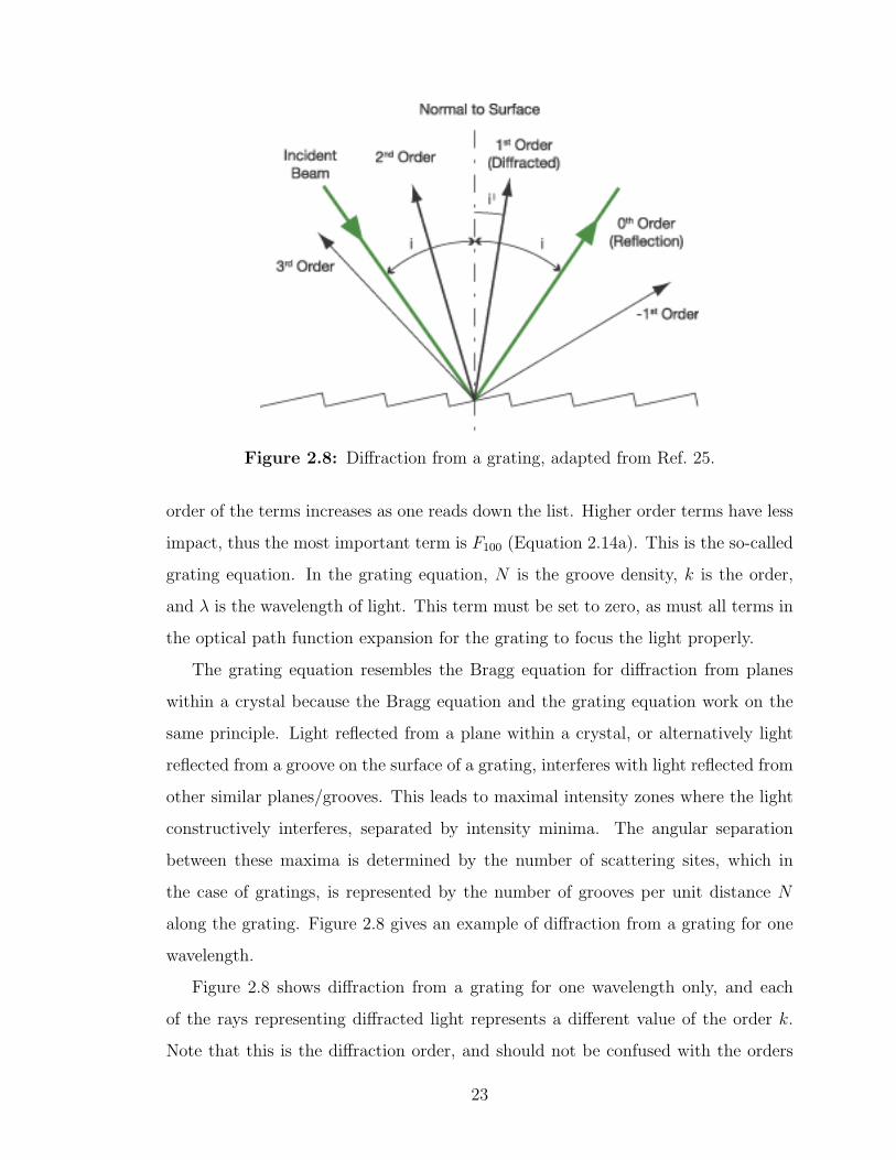
Figure 2.8: Diffraction from a grating, adapted from Ref. 25.
order of the terms increases as one reads down the list. Higher order terms have less
impact, thus the most important term is F100 (Equation 2.14a). This is the so-called
grating equation. In the grating equation, N is the groove density, k is the order,
and λ is the wavelength of light. This term must be set to zero, as must all terms in
the optical path function expansion for the grating to focus the light properly.
The grating equation resembles the Bragg equation for diffraction from planes
within a crystal because the Bragg equation and the grating equation work on the
same principle. Light reflected from a plane within a crystal, or alternatively light
reflected from a groove on the surface of a grating, interferes with light reflected from
other similar planes/grooves. This leads to maximal intensity zones where the light
constructively interferes, separated by intensity minima. The angular separation
between these maxima is determined by the number of scattering sites, which in
the case of gratings, is represented by the number of grooves per unit distance N
along the grating. Figure 2.8 gives an example of diffraction from a grating for one
wavelength.
Figure 2.8 shows diffraction from a grating for one wavelength only, and each
of the rays representing diffracted light represents a different value of the order k.
Note that this is the diffraction order, and should not be confused with the orders
23

of harmonics discussed earlier with respect to insertion devices. The diffraction
angle i′ depends upon wavelength as well as order, so that for a particular order
the radiation incident upon the grating is split into a wide angular fan according to
wavelength. If one aligns the optics according to a particular diffraction angle, the
unwanted wavelengths of light will focus off-axis. The exit slit, which functions in
much the same fashion as the entrance slit, absorbs the off-axis radiation and allows
only the desired bandwidth to pass. As with the entrance slit, a smaller slit width
will eliminate a larger section of the radiation fan that is diffracted from the grating.
In doing so, however, the flux impinging on the sample is limited. Note that the
fan effect only applies to the first order and higher. In the case of the zeroth order,
the first term in the grating equation is 0 for all wavelengths. This is simply light
reflected off the plane of the grating with no angular dependance on wavelength.
The differing angles of diffraction for wavelengths scattered from the grating in-
troduces an interesting problem into beamline design. The dependance of diffraction
angle on wavelength means that the focal length is also dependant on wavelength.
With this problem in mind, the exit slit for the monochromator at Beamline 8.0.1
was built to move along the optical path, thus changing its separation distance from
the grating to coincide with new focal lengths. Without this function, the exit slit
may be too close or too far from the grating, depending on the desired photon energy.
In addition to the movable exit slit, the grating can be rotated. These functions in-
crease the energy range that the monochromator can reach and still have it bring a
respectable flux rate to bear upon the sample. Although this design increases the
energy window that the beamline can access, it nevertheless can in principle skew
energy calibration if the exit slit of the monochromator is not placed in precisely
the correct spot to allow through photons with the desired energy. This problem is
correctable, provided that the energy calibration error does not change noticeably
over an excitation threshold. If the energy calibration error is constant, then the
spectrum can simply be shifted to the appropriate energy. This shift is calculated
by comparing the spectrum of a commonly measured standard sample to its ac-
cepted spectrum presented in literature. Of course, the spectrum of this standard
24

sample must be measured with the same set of parameters as the sample(s) under
investigation, and its spectrum must be within the same energy range.
Figure 2.8 shows a wide angular separation between the orders of radiation that
are diffracted from the grating. This is done to make the figure readable and in-
structive, but it is misleading because such large angles with respect to the surface
of the grating are not possible in soft x-ray optics. All soft x-ray optical systems
require the optics to aligned using grazing angles of incidence. This constraint is
necessary simply because soft x-rays interact very strongly with matter, so grazing
incidence is required to maximize the reflected portion of the radiation. This high
level of interaction with matter is also the reason why soft x-ray beamlines require
the optical path to be in ultra high vacuum (UHV).
2.2.2 The Endstation
The endstation is the term used to describe the systems necessary to hold the sam-
ple and keep it in UHV, as well as all of the instrumentation that is necessary to
document how the sample reacts to the radiation that has been focused upon it.
This part of a beamline is by far the most variable component, as there are several
different ways that matter can react to radiation, and for each of these radiation-
matter interactions there can be many experiments that can record the event, each
in a different way. Thus, the configuration of, and the instrumentation used with,
an endstation can vary substantially among beamlines, even beamlines that operate
within the same energy range. As with the discussion of monochromators above,
the topic of endstations will be concerned largely with Beamline 8.0.1; specifically,
the Soft X-ray Fluorescence (SXF) endstation. However, the SXF endstation is not
entirely unique, and variations of the instruments found therein can be found on
other endstations.
There are many components to the endstation, such as the mechanisms that allow
one to transfer samples into the measurement chamber. The present discussion will
be limited to those components necessary to measure XAS and RIXS spectra. These
components are a highly transparent gold mesh, the sample plate, the spectrometer,
25

and a Channeltron detector. The first three will be discussed later in this section
on endstation design. The function and application of the Channeltron, however, is
discussed in detail in the Total Fluorescence Yield section of Chapter 3. Suffice is to
say here that the Channeltron is used to measure a large portion of the total number
of photons that are emitted from a sample when it is excited at a particular energy.
The second component to be discussed, the gold mesh, comes before the sample,
in the sense that the beam passes the mesh before reaching the sample. It does not
measure how the sample reacts to the incoming radiation per se, but it is neverthe-
less necessary for a proper analysis of any measured XAS spectrum. The purpose
of the gold mesh is to measure the intensity of the incoming beam before it hits
the sample. The gold mesh is connected to ground through a picoammeter. The
picoammeter measures the amount of current that is flowing into the mesh from
ground as electrons are removed because of interaction with the radiation beam.
The physics that dictate how the electrons are removed from the mesh is discussed
in the Total Electron Yield section in Chapter 3. The current that is flowing into
the mesh increases with the intensity of the beam, simply because more electrons
are removed. Thus, the mesh current shows the intensity of the radiation that the
sample is receiving at that energy and bandwidth, relative to other energies. Ideally,
the mesh itself is a material that has a constant probability to absorb the photons
across the energy range of interest, so that the experimentalist knows the intensity
of radiation explicitly without needing to be concerned with the details of how the
mesh is interacting with the radiation.
Gold is a popular choice for mesh materials because it does not react strongly
with any other element, including oxygen. Thus, a pure gold mesh stays relatively
pure, making it highly effective because there are only the various gold resonant
absorption edges to cause concern. Over time, elements such as carbon will build up
on the gold mesh despite the relative chemical inertness of gold. This problem can be
overcome by evaporating more gold onto the mesh, covering the contaminants. This
can be done in situ, which minimizes contamination because the beamline does not
have to be vented to replace the mesh. Also, gold is a good conductor, facilitating
26

the replacement of electrons that have been removed.
The mesh current is important information when performing a measurement
that requires scanning across an energy range. At each photon energy, the flux
that is reaching the sample is measured, and a spectrum is recorded of the mesh
current as a function of photon energy. This is necessary to record because the
beamline itself interacts with the beam, absorbing more photons at certain energies if
they happen to correspond to the energies of resonant absorption edges of materials
found within the beamline. These materials may be put there deliberately, such
as the SiO2 that is commonly used to make mirrors. However, the beamline may
also have some contamination. This contamination may be from gases in the non-
ideal vacuum in the beamline, but contaminant solids may also have reacted with
the reflective/diffactive surfaces within the beamline. Regardless of the source, the
effects of the contaminants must be removed because they superimpose structure on
the spectrum that is measured from the sample.
If there is a material in the beamline that absorbs photons preferentially at a
certain energy, then a drop in the mesh current will be observed at that energy.
This structure is removed simply by dividing the spectrum of the sample by the
mesh current, called normalization. The normalized spectrum will therefore display
only the spectral structure of the sample over the energy range in question, with
no contribution from the beamline. Normalizing the absorption spectrum to the
mesh current also removes any fluctuations in the intensity due to the storage ring.
To summarize, normalizing the absorption spectrum to the mesh current makes the
spectrum independent of the spectral curves of all materials preceding the sample.
The next component is the sample holder. Other than performing the necessary
and obvious job of holding the sample in the path of the beam, the sample holder is
also grounded through a picoammeter. This allows one to measure the rate at which
electrons are being replaced in the sample. This is much the same as the system set
up to measure the mesh current. The details of this experimentation technique are
discussed in the Total Electron Yield section of Chapter 3.
The last component to be discussed on the endstation of Beamline 8.0.1 is the
27

spectrometer. When radiation interacts with matter, that radiation may transfer
energy to the matter. The substance may then de-excite by releasing a photon to
carry away the excess stored energy. This is called a photon-in photon-out process,
and the purpose of the spectrometer is to detect and analyze the outgoing photons.
The Channeltron does this as well, however the Channeltron measures the photon
count rate as a function of excitation energy, whereas the spectrometer measures
the emitted photons as a function of emission energy. The spectrometer consists of
three components: an entrance slit, a grating, and a photon detector. As before
in the monochromator design, narrowing the slit will increase energy resolution but
will decrease the flux illuminating the grating and ultimately the photon detector.
The photons that are emitted from the sample and pass through the entrance slit
shine on the grating, which splits the different wavelengths. It functions in this
way much like the monochromator, however the spectrometer has a much different
purpose. The various wavelengths of light emitted by the sample, separated by
the grating, are then focussed onto an area sensitive photon counter, such as a
charge coupled device (CCD) or a multi-channel plate (MCP). The spectrometer on
Beamline 8.0.1 uses an MCP. The photon detector must be area sensitive because the
wavelengths of light will focus onto different parts of the sensor. The range of energies
which the sensor may detect, called the energy window, is therefore determined
largely by the size of the detector and the angular separation between different
wavelengths produced by the grating. As a rule, however, photons with longer
wavelengths (smaller energy) have greater angular separation than photons with
shorter wavelengths (higher energy). Thus, the window for low energy photons is
smaller, but in exchange the resolution is better for low energy photons because it
is easier to spatially differentiate between wavelengths.
The spectrometer on the SXF endstation of Beamline 8.0.1 is designed according
to Rowland circle geometry. Rowland circle geometry is the result of a theoretical
analysis performed by H. A. Rowland before the optical path function had been
derived from Fermat’s principle. His goal was to minimize the aberrations incurred
when using a spherical grating [26]. The grouping of the terms in Equation 2.14
28

allows one to easily see that there are parts common to Equations 2.14c, 2.14d, and
2.14e. The terms common to all three equations are as follows:(cos2 i
r− cos i
R
)and
(cos2 i′
r′− cos i′
R
)(2.15)
If one sets these two terms to zero and solves for r and r′, then the solution is:
r = R cos i and r′ = R cos i′ (2.16)
These are called the Rowland conditions. The conditions require that the source
and target (the entrance slit and MCP, respectively) lie upon a circle of radius R,
called the Rowland circle. In addition, the spherical grating must have a radius of
curvature of 2R. If these conditions are met, then the first five terms of the optical
path function reduce to the following equations:
F100 = Nkλ− (sin i+ sin i′) (2.17a)
F020 =1
r+
1
r′− 1
R(cos i+ cos i′) (2.17b)
F200 = 0 (2.17c)
F300 = 0 (2.17d)
F400 = − 1
R3(cos i+ cos i′) +
1
R2
(1
r+
1
r′
)(2.17e)
Thus, simply by keeping the source, grating, and sensor on the Rowland circle,
the F200 and F300 terms are made identically 0, and the fifth term, F400, is signifi-
cantly reduced. Provided that one can design a spectrometer with Rowland circle
geometry that can also accommodate grazing angles of incidence, then the product is
a spectrometer that is affected little by the most influential aberrations. Care must
still be taken to properly focus the image in the sagittal plane, which is the focal
element controlled by Equation 2.17b. Figure 2.9 below gives a visual representation
of a spectrometer that is built using Rowland circle geometry.
The high brilliance of synchrotron sources is of paramount importance when
using a spectrometer to record photon-in photon-out processes. Before the photon
beam even reaches the sample, it must pass over two or more mirrors, as well as
29

Figure 2.9: A spectrometer design that adheres to Rowland circlegeometry. The entrance slit and photon sensor must remain on thecircle, although they are free to move anywhere along it.
pass through two slits and at least one grating. Each of these components, the slits
especially, throw away photons. When it hits the sample, the flux of the photon beam
is a small fraction of what the insertion device produced. The sample, now excited,
must have its excited atoms decay and produce photons. As will be discussed later,
however, the probability that the sample will shed energy by radiative decay is quite
low in the soft x-ray regime. To make matters worse, the photons produced by the
sample radiate in all directions equally, so that only a very small solid angle of the
emitted photons strike the entrance slit of the spectrometer. Once the photons are
past the entrance slit, they must pass over a grating which further cuts the intensity
as it absorbs photons. Taken all together, even an expertly designed beamline is
highly inefficient. Thus, nothing less than the very brightest sources can deliver a
sufficiently high signal-to-noise ratio for photon-in photon-out experiments.
Much of the information concerning the optical components of a beamline, namely
the slits and gratings that are found within spectrometers and monochromators, was
presented in the work of W. B. Peatman [27].
30

Chapter 3
Experimentation Techniques
3.1 X-ray Absorption Spectroscopy
X-ray absorption is the process during which an incoming photon is absorbed by an
atomic site within the crystal; x-ray absorption spectroscopy (XAS) measures this
process. The energy is absorbed primarily by the electron cloud, where it is used to
promote electrons from their ground state into unoccupied states. If the absorbed
photon energy and the binding energy of the electron are nearly equal, then the
electron will be promoted to previously unoccupied bound states within the crystal,
such as the conduction band. These bound states may be localized to the atomic
site from which the electron was promoted, or they may be delocalized, allowing
the electron to move somewhat freely within the crystal. However, if the excitation
energy is much greater than the binding energy of the electron, then the electron
may be promoted to unbound states. The electron becomes a free particle.
It is possible to promote any electron, provided that the absorbed photon had
energy greater than the energy required to complete the transition. There are many
possible transitions, but not all will have equal probabilities of occurring. Selec-
tion rules determine which type of radiative absorption process will dominate for
a given excitation path; the possible processes are electric dipole-allowed, electric
quadrupole-allowed, or magnetic dipole-allowed transitions. The transition proba-
bility for an electric dipole transition is generally at least three orders of magnitude
greater than electric quadrupole- or magnetic dipole-allowed transitions. The selec-
tion rules for an electric dipole transition are listed in Table 3.1.
The selection rules in Table 3.1 apply in the case of Russells-Saunders coupling,
31

Table 3.1: Electric Dipole (E1) Selection Rules
∆S = 0
∆L = 0,±1
∆J = 0,±1
∆Mj = 0,±1
also called LS coupling. The S, L, and J letters in Table 3.1 refer to the spin,
orbital angular momentum, and total angular momentum quantum numbers that
describe the state of the atom. When LS coupling holds, the spins of the electrons
are well-defined, as are the orbital quantum states. One can think of the selection
rules for spin and orbital angular momentum as a consequence of the requirement for
conservation of momentum. A photon has quantized spin, and the quantum number
that describes the spin is 1. When an atom absorbs a photon, the quantum of spin
of the photon must be accounted for, so the orbital angular momentum state of the
atom must change by 1. However, the total spin cannot change. The total angular
momentum selection rule is a consequence of the weak coupling of electron spin and
orbital angular momentum.
The energy of the exciting photon is also a crucial factor in determining which
of the possible transitions are most likely to occur. If the energy of the photon is
equal or close to the energy of a transition, this excitation process will be prefer-
entially populated over all other possible excitation paths. This is called resonant
excitation. This property gives XAS site-selective, symmetry-selective, and element-
specific properties because the binding energies for the core electron shells of a given
element are unique to that element alone. During an XAS experiment, one can ex-
cite one element in a compound at its core electron threshold without fear that the
spectra will become contaminated with spectral weight from the other elements.
X-ray absorption spectroscopy probes the unoccupied states of the atomic site
that one is exciting. This is due to the so-called final-state rule, which states that the
probability that a certain transition will occur, and the energy at which it occurs,
is dominated by the final state configuration of the atom. The final state of an
32

atom after absorbing a photon has a hole in a core shell and, in the case of resonant
excitation, an extra electron in the previously unoccupied states. Because of the
final-state rule, XAS probes the unoccupied states of the atom.
There are different ways to measure an XAS spectrum, and three of these methods
will be discussed here. The first technique is total electron yield (TEY). The other
two techniques of note are total fluorescence yield (TFY) and partial fluorescence
yield (PFY). All three techniques are unique in that they use different detection
methods to probe how efficiently the sample is absorbing the incident photons.
3.1.1 Total Electron Yield
The total electron yield (TEY) technique measures the rate at which electrons are
replenished within the sample. This technique takes advantage of Auger decay pro-
cesses, which strongly compete with radiative decay processes in the soft x-ray energy
range. Simply stated, during an Auger relaxation event, the energy released when the
core hole is refilled is transferred to another electron with the same principle quan-
tum number. This energy is sufficient to ionize the atom and create a free electron.
The possible relaxation paths that may be populated are shown in Figure 3.1.
Figure 3.1: Possible Auger relaxation paths
33
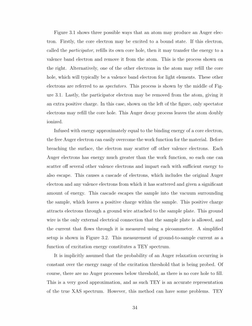
Figure 3.1 shows three possible ways that an atom may produce an Auger elec-
tron. Firstly, the core electron may be excited to a bound state. If this electron,
called the participator, refills its own core hole, then it may transfer the energy to a
valence band electron and remove it from the atom. This is the process shown on
the right. Alternatively, one of the other electrons in the atom may refill the core
hole, which will typically be a valence band electron for light elements. These other
electrons are referred to as spectators. This process is shown by the middle of Fig-
ure 3.1. Lastly, the participator electron may be removed from the atom, giving it
an extra positive charge. In this case, shown on the left of the figure, only spectator
electrons may refill the core hole. This Auger decay process leaves the atom doubly
ionized.
Infused with energy approximately equal to the binding energy of a core electron,
the free Auger electron can easily overcome the work function for the material. Before
breaching the surface, the electron may scatter off other valence electrons. Each
Auger electrons has energy much greater than the work function, so each one can
scatter off several other valence electrons and impart each with sufficient energy to
also escape. This causes a cascade of electrons, which includes the original Auger
electron and any valence electrons from which it has scattered and given a significant
amount of energy. This cascade escapes the sample into the vacuum surrounding
the sample, which leaves a positive charge within the sample. This positive charge
attracts electrons through a ground wire attached to the sample plate. This ground
wire is the only external electrical connection that the sample plate is allowed, and
the current that flows through it is measured using a picoammeter. A simplified
setup is shown in Figure 3.2. This measurement of ground-to-sample current as a
function of excitation energy constitutes a TEY spectrum.
It is implicitly assumed that the probability of an Auger relaxation occurring is
constant over the energy range of the excitation threshold that is being probed. Of
course, there are no Auger processes below threshold, as there is no core hole to fill.
This is a very good approximation, and as such TEY is an accurate representation
of the true XAS spectrum. However, this method can have some problems. TEY
34

Figure 3.2: Simplified setup for a TEY experiment
measures the rate at which valence holes are replenished within the sample, which
depends upon the conductivity of the sample. Conductivity can be assumed to be
constant over the whole threshold, but poor conductivity, when measuring highly
insulating materials, can lead to poor count rates and possibly to sample charging.
Sample charging occurs when the electrons that are ejected into space cannot be
replenished quickly enough by an external source. The sample builds a positive
charge, which increases the amount of energy that electrons require to break free
of the sample. In short, the work function is not constant across the scanned en-
ergy range. Sample charging is easily recognized by a noticeable, often steep drop
in the measured ground-to-sample current. This drop is due to the inability of the
Auger electrons to break free of the increasingly steep positive potential well, which
leads to lower count rates. The positive charge on the sample is sufficient to inhibit
photoelectrons from leaving the surface, but it is not enough to increase the current
because the potential is not great enough to cause dielectric breakdown. Dielec-
tric breakdown would of course be undesirable, as it would significantly distort the
electronic structure of the sample.
TEY is also highly sensitive to surface effects. The electrons that are produced
by the Auger process have a short mean free path length, on the order of a few
Angstroms, which means that the electrons cannot travel far within the crystal
without interacting with the lattice. Electrons produced by deep-lying atoms are
35

recaptured by the crystal before escaping into space. Thus, electrons that exist
in surface states tend to dominate a given TEY spectrum. This is problematic for
metastable or highly reactive systems, such as the pure transition metals that oxidize
very quickly upon exposure to atmosphere.
3.1.2 Total Fluorescence Yield
The problems inherent to TEY can be overcome to a certain extent by using the total
fluorescence yield (TFY) technique. The TFY technique differs from TEY in that it
measures the photons that are emitted from the sample when the atoms radiatively
de-excite. This is very different from TEY, which depends upon the Auger process
in which the energy of the excited state is carried away by an electron. A TFY
experiment typically uses a Channeltron, a device that records the electron cascade
that occurs when a photon interacts with the detector. Since electrons that strike
the detector can cause a similar electron cascade, the Channeltron has a bias voltage
that repels any electrons that are emitted from the sample. The spectrum produced
by an absorption experiment measured in TFY mode is simply the number of counts
that the Channeltron recorded as a function of excitation energy.
The TFY experimentation technique records the photons emitted from the sam-
ple, which has both its advantages and its disadvantages. The upside of TFY is
that it has better penetration depth, because photons penetrate more deeply than
electrons. This removes the problem of surface effects dominating the measured ab-
sorption spectrum. Also, TFY is the technique of choice when dealing with highly
resistive materials, as sample charging is not a relevant problem. The downside of
TFY is that it senses emitted photons. In the soft X-ray energy range, Auger and
radiative processes compete to refill the core hole, and the Auger decay channel
strongly dominates, especially with the lighter elements. Thus, TFY can have a pro-
hibitively poor signal-to-noise ratio simply because the probability of a photon being
produced is so small, relatively speaking. There is also the problem of self-absorption.
Self-absorption is difficult to take into account because it is not uniform across the
entire threshold; the more intensely photons are radiated at a certain energy, the
36
more strongly those photons are absorbed by other atomic sites in the crystal as the
photons attempt to escape the crystal. Thus, TFY spectra inherently have skewed
intensity profiles, as the most intense peaks seen in the spectrum should be even
larger if self-absorption was not present. When using a Channeltron to record TFY
spectra, problems may arise because of the bias voltage of the Channeltron. The
bias voltage is necessary to keep the Auger electrons away from the detector, but if
the voltage is set too high, it may distort the electronic states of the crystal. Despite
these limitations, however, the TFY technique can produce excellent spectra that
are much more representative of the bulk states than a TEY experiment.
TFY and TEY share a common property in that any spectrum that is recorded
using one of these two methods is not simply an absorption spectrum of the core
threshold this one is resonantly exciting, but rather a spectrum of all thresholds
accessible at that excitation energy. For example, consider an iron oxide compound.
The L2,3 edge of Fe requires photons of approximately 705 eV to begin resonantly
exciting the 2p electrons. At this energy, however, it is in principle possible to excite
the 1s electrons of the O ions that share the crystal, given that the K edge on
O only requires ≈510 eV. Of course, photons with energies around 705 eV will not
resonantly excite the K edge of oxygen; the probability of producing a 1s core hole on
O is minuscule compared to the probability of created a 2p hole on Fe. Nevertheless,
it can still happen. The Channeltron detects any photon that fits within its energy
detection window, even if it was not produced though decay of the core hole that
is being resonantly created. As a result, TFY spectra, and similarly TEY spectra,
sit upon a substrate of signal produced by the decay of lower energy core holes that
were produced non-resonantly as the incident radiation strikes ligand states.
This appears easy to correct. It seems logical to assume that the cross-section
for the O K edge, in this example, will remain unchanged as one encounters the Fe
L2,3 edge. After all, the Fe L2,3 edge is nearly 200 eV above the O K edge, which is
well beyond any possible multiplet effects due to the O site. However, this is not the
case. Experiments that probe the photoemission yields at a higher lying threshold
on one element while exciting a deeper core level on another element within the
37

same crystal clearly show that the number of photons produced though decay of
higher-lying core holes is dramatically curtailed as a deeper core level is resonantly
probed [28]. Thus, TFY and TEY spectra are in principle highly complicated spectra,
with components from higher-lying core thresholds varying just as much as the signal
from the threshold under scrutiny. However, most of the time the background signal
is negligible, and the signal from the decay of the resonantly created core holes far
outweighs all other components.
3.1.3 Partial Fluorescence Yield
Partial fluorescence yield (PFY) is a third technique that can be used to measure
XAS. Like TFY, the PFY technique measures the photons that are produced by the
sample. PFY has all the aforementioned advantages and disadvantages of the TFY
technique. Unlike TFY, however, the photons are detected using a spectrometer. It
is unnecessary for a spectrometer to have a bias voltage to repel emitted electrons,
so there is no danger that the spectrometer will affect the electronic states of the
sample.
When measuring a TFY spectrum, the Channeltron simply counts the number
photons that strike the sensor. However, the spectrometer has its own transmission
efficiency because the fluorescence photons must pass an entrance slit and a grating,
and as such a lot of flux is lost in the process of producing a PFY spectrum. This
generally means that PFY spectra have the poorest signal-to-noise ratio of all three
techniques discussed thus far. The problem of low emitted photon flux can be mit-
igated somewhat by increasing the incident photon flux. However, this invariably
reduces the resolution of the resultant spectrum.
Although the spectrometer does significantly decrease the signal-to-noise ratio,
the energy detection window of the spectrometer is very much smaller than those
of the Channeltron or the picomammeter. This gives the PFY technique a property
that sets it distinctly apart from TEY and TFY: a PFY spectrum does not measure
extraneous signal produced by the decay of holes other than the ones resonantly
created. The detection window can be tuned to a particular transition energy range.
38

This allows the experimentalist to know explicitly what it is that he is measuring,
even if the spectrum that is being measured takes an exceedingly long time to acquire.
3.2 X-ray Emission Spectroscopy
X-ray emission spectroscopy (XES) measures the photons that are emitted from the
sample using a spectrometer. Just as for XAS, the final-state rule applies to XES as
well, except that in the final state of all XES events, there is no core hole and one
hole in the valence band. XES techniques therefore probe the occupied states, as the
multiplet effects from the new hole in the occupied states gives an XES spectrum its
shape. The physical mechanism that produces the photons, however, can be quite
different depending on how close the energy of the exciting radiation is to a core
hole excitation threshold. Excitation energies that are relatively far above threshold
produce non-resonant XES spectra, whereas at excitation energies that are near-
or on-threshold, the dominant process is resonant inelastic x-ray scattering (RIXS).
Both of these mechanisms are photon in-photon out process, and are displayed in
Figure 3.3.
Simple XES can, in principle, happen at all excitation energies. XES is a two-step
process; the first step is the creation of a core hole. The photons measured in XES are
produced when the core hole is refilled by either the participator electron or another
spectator electron. The relevant spectator electrons are the valence electrons. In
principle, any electron can refill the core hole, provided that the necessary transition
satisfies the dipole selection rules, but the emitted photons are too low in energy to
be seen within the detector window of the spectrometer. The left panel in Figure 3.3
shows the total process. Note that the figure shows that the electron is promoted
to the unoccupied states. While this is in general true, XES is most probable in the
non-resonant case at excitation energies far above threshold. In this case, the core
electron is removed from the atom, leaving the atom ionized.
RIXS is the photon-out process which is the more likely for on-threshold energies.
RIXS is a one-step scattering process, wherein the scattering transition is the net
39

Figure 3.3: Photon-in photon-out processes. The left panel representssimple fluorescence, or XES. The photon that is emitted has energyequal to the decay of the core hole. The right panel shows the nettransition of a RIXS event. The photon that is emitted is the excitationenergy with the energy of the net transition subtracted from it.
result of virtual core hole creation and annihilation events [29]. The right panel
in Figure 3.3 displays a RIXS event; the dashed lines are the virtual transitions,
whereas the solid line is the transition that physically occurs. A RIXS event is
the result of two independent dipole-allowed events, and as such, the selection rules
for high-probability net transitions are slightly modified. The spin selection rule
remains the same (∆S = 0), but angular momentum selection is altered to become
∆L = 0,±2. This allows one to efficiently probe inner-shell transitions.
Although XES and RIXS events each have the same final state, i.e. an electron
in the conduction band and a hole in the valence band, the physical mechanism that
promoted the electron differs greatly between the two processes. In XES, the photon
that is detected by the spectrometer has energy equivalent to the energy separation
of the valence and core states, because the photon is created to carry away the energy
that is released when the core hole is annihilated. This energy separation does not
40

change with excitation energy. This will have the effect that inelastic XES peaks
will maintain a constant energy, even though the elastic peak will track with the
excitation energy. This concept is displayed in Figure 3.4(a).
RIXS features, however, are quite different. The energy losses in RIXS typically
correspond to the transition in which valence electrons are scattered to unoccupied
states; the total energy necessary to complete the net transition is always the same
for a given scattering transition. This energy is subtracted from the energy of the
photon that is exciting the atom. The photon that is sensed by the spectrometer has
an energy that is the original excitation energy minus the energy required to complete
the transition. Thus, a feature that maintains the same energy separation from the
elastic peak, regardless of excitation energy, is an inelastic scattering peak. An
example of the evolution of an inelastic scattering feature is shown in Figure 3.4(b).
The probability that a RIXS event will occur is determined by the Kramers-
Heisenberg formula. The Kramers-Heisenberg formula was originally derived without
the use of quantum mechanics by H. A. Kramers and W. Heisenberg to describe the
scattering of a photon by an atomic electron, but was later derived using quantum
mechanics by Dirac [30, 31]. The Kramers-Heisenberg formula for the intensity of a
scattered photon at a particular emission energy Eout is shown below:
I(Ein, Eout) ∝∑
f
∣∣∣∣∣∑m
〈f | f · A |m〉 〈m| f · A |i〉Em − Ei − Ein − iΓ
2
∣∣∣∣∣2
δ(Ef + Eout − Ei − Ein) (3.1)
where the symbol E refers to energy, with the subscripts f , m, and i refer to the
final, intermediate, and initial states, respectively. The subscripts in and out refer
to the incident and scattered photons.
The Kramers-Heisenberg formula has two parts that require explanation. Firstly,
there is the numerator, which is the product of two matrix elements. One matrix
element represents the dipole-allowed transition from an initial state to an interme-
diate state, and the second matrix element is the dipole-allowed relaxation of that
intermediate state to a final state. The denominator is the second part of note,
and its function is to magnify the intensity of the inelastic process described by
41

Figure 3.4: Examples of XES and RIXS peaks in experimental spec-tra. These spectra are not real, but have been simulated to exemplifythe expected behavior of typical soft x-ray photon-out processes. Eachspectrum in each panel corresponds to a different excitation energy.
the numerator when the excitation energy, Ein, comes near to the energy difference
between the intermediate and initial states, Em − Ei. To prevent the denominator
from becoming undefined, an imaginary quantity Γ has been introduced, which is
the lifetime broadening of the intermediate state. The denominator describes the
resonance part in the term ‘resonant inelastic x-ray scattering’.
RIXS, in particular, is a very powerful technique for studying the density of states
of a system. Inelastic scattering features maintain a constant energy separation
from the elastic peak. This energy is characteristic of the net transition. This
gives information about the partial DOS, because each inelastic energy loss feature
42

represents a transition between a local maximum in the occupied states and a local
maximum in the unoccupied states. Thus, one can get specific information about
the electronic structure.
Another benefit is that RIXS is element-specific. This is because a RIXS feature
is the net result of two virtual transitions, one of which is core hole creation, a process
that is characteristic of the element in question. This property allows one to probe
site-specific states without spectral weight from other elements contributing to the
measured spectrum. Optical absorption similar to RIXS, because both techniques
have the same net transition and thus probe the same states. Optical absorption
is superior for determining DOS fine structure that cannot be resolved using RIXS,
however, optical absorption probes the near-Fermi edge DOS of every atomic site
in the entire crystal. The element-specific RIXS technique allows one to probe the
local DOS of only the resonantly excited element, although that local DOS will have
some structure that results from inter-atomic interaction.
43
Chapter 4
Electronic Structure of Solids
4.1 Band Structure Basics
The physics of condensed matter marks a strong departure from the physics of the
comparatively simpler atomic picture. The most obvious difference is that a given
atom in the solid is not in a spherically symmetric environment. Electrons from
neighboring atoms interact with each other, and charge clouds overlap to form bonds.
In addition, if one considers a crystalline sample, wherein the atoms have bonded
with long-range ordering, then the electronic structure shows periodic structure.
Theory pertaining only to the electronic structure of crystals will be considered in
this thesis, although in principle matter can condense in a completely unstructured
(amorphous) phase.
The periodicity of the structure within a crystal, both physical and electronic,
lends itself conveniently to Fourier analysis, as Fourier analysis involves expanding
a function in terms of periodic functions, most commonly sinusoids. As an example,
the electronic charge density n(r) can be expanded in the following Fourier series:
n(r) =∑
G
nG exp(iG · r) (4.1)
In this expansion, G is the reciprocal lattice vector, defined by the relation G ·
T = 2πn, where n is an integer and T is the translation vector of the crystal
lattice. The reciprocal lattice is a powerful concept, as it represents the crystal
lattice transformed into crystal momentum space, or k-space as it is more commonly
called. One important property to note is that the length of k-space and real space
44

vectors reciprocally scale with respect to one another. Thus, a large r-space vector
transforms into a short k-space vector, and vice versa.
The Bloch theorem states that solutions to the Schrodinger equation in a periodic
potential must also be periodic. These solutions have the form:
ψi,k(r) = ui,k(r) exp(ik · r) (4.2)
where k is a reciprocal lattice vector, and i gives the state that the wavefunction is
describing, including symmetry labels and quantum numbers. This formula shows
that for a certain wavevector k and state i, there is only one possible solution to
the Schrodinger equation, and thus one energy eigenvalue that can be observed.
Other states may exhibit this energy at the same wavevector, if they are degenerate.
However, each eigenvector can only have one eigenvalue for each k. Recalling the
periodicity of a crystal, each translationally invariant atom within the crystal will
provide electrons with the same state, but with different values of k. Because k-space
vectors and r-space vectors scale reciprocally, solutions to the Schrodinger equation
with index k are possible every 2π/N wavevectors, where N is the number of atoms
in the crystal. Therefore, as the number of atoms in the crystal increases, eigenvalues
εi,k are nearly continuous with k for state i.
Another way of looking at it is to consider what happens when identical atoms
are brought close enough such they may interact with one another, and are arranged
in a periodic fashion. As the valence electrons on each site begin to interact, the
problem arises that the electrons that occupy the same orbitals on different atoms
are no longer unique. The orbitals that these electrons occupy are exactly the same
within an integer number of lattice translations. This is not acceptable, as no two
electrons can occupy the same orbital at the same time. The solution is to modify
the wavefunctions of the valence electrons such that they are no longer orthogonal,
which allows the valence electrons to coexist. The result is valence electrons that
have the same electronic environment but have different energies, depending on their
momentum.
Either way that one looks at it, the result is the same. The interaction amongst
45

electrons in an extended solid produces continuous band structure, with the energy
of the band varying as a function of k. Band structure calculations are powerful
analytical tools, as they predict the energies of the transitions that are possible
given a certain symmetry axis. However, one can also look at the electronic density
of states (DOS) as a meaningful representation of the electronic structure of a crystal.
The band structure and the density of states of a crystal are related simply through
the following formula:
D(E) =V
(2π)3
∫dSE
|∇kE(k)|(4.3)
where SE is a surface area element on a constant energy surface of the three di-
mensional band structure, and ∇kE(k) is the gradient of the band structure with
respect to k. The important property to note here is that the density of states is
inversely proportional to the gradient of the band structure. A flat band produces
a sharp peak in a graph of the DOS at that energy, whereas a band with a lot of
structure will produce broad features in the DOS. Of course, a large gradient with
respect to k within a band suggests a large degree of electron cloud interaction as
per the discussion above. Thus, a graph of the density of states gives a visual and
intuitive look at the level of interaction that the band in question is experiencing.
Although the presence of band structure is a result of the periodicity of the crys-
tal, determining the shape of the band structure is a very complicated problem. As
stated above, the shape of the band, and therefore the density of states, is directly
dependant upon the symmetry and magnitude of the interactions amongst the elec-
tron clouds of the atoms, as well as the interactions between the electrons and the
fixed atomic nuclei. There have been many attempts to understand and simulate the
dynamics of a crystalline system. The orthogonalized linear combination of atomic
orbitals (OLCAO) method was used to simulate LiFePO4, a subject that will be dis-
cussed later in this chapter. This method is based upon the formalisms introduced
by the local density approximation (LDA) of density functional theory (DFT).
46

4.2 Density Functional Theory
Density functional theory was formulated by Hohenberg and Kohn as an exact theory
for many-body interactions. The guiding principle behind DFT is a deceptively sim-
ple one: All properties in a solid, including (but not limited to) electronic excitations,
thermal and electrical conductivity, and magnetic susceptibility are all functionals
of the ground state electron charge density. If one knows the ground state electron
charge density, then one could in principle calculate all other macroscopic properties
of a solid with this information alone.
The following formula is the Hamiltonian proposed by Hohenberg and Kohn.
H = − h2
2me
∑i
∇2i +
∑i
Vext(ri) +1
2
∑i6=j
e2
|ri − rj|(4.4)
The first term in this Hamiltonian is simply the kinetic energy operator. The second
term takes into account any external fields, including all fields that are not generated
by the electrons within the crystal. This term must account for the Coulomb electric
field produced by the fixed ionic lattice, but in principle this term may also include
fields generated outside of the crystal. The last term explicitly accounts for two-
electron Coulomb interactions. Depending on the wavefunctions upon which this
Hamiltonian operates, the interactions can be of the direct, exchange, or correlation
type.
According to the Hohenberg-Kohn theorems, the external potential is uniquely
determined by the ground state particle density, which will be stated here without
proof. The kinetic energy term and the electron-electron interaction term are by
definition unique to a particular electron density, and so the full Hohenberg-Kohn
Hamiltonian is uniquely determined for a particular electron density. The total
energy, which is simply the observable eigenvalue of the full Hamiltonian, is also
uniquely determined by a given electron density. The density that minimizes the
total energy is, by definition, the ground state particle density. The total energy is
given as follows:
47

EHK [n] = T [n] + Eint[n] +
∫d3rVext(r)n(r) + EII (4.5)
The third term is the energy of the interaction between the electrons and the
fixed ionic lattice. The fourth term is simply the energy of the ions interacting with
one another, hence the II subscript. These are straightforward to calculate, if one
knows the density. The first term is the total kinetic energy, and the second term
is the so-called internal energy, which is the energy that is inherent in the electron-
electron interaction. The first and second terms are much more difficult to calculate
than the third and fourth terms, for different reasons. The main problem arises from
the kinetic energy term. At present, there is no known way to calculate the kinetic
energy directly from the electron charge density.
Despite its intractability, the Hohenberg-Kohn Hamiltonian is nevertheless exact.
The Hohenberg-Kohn Hamiltonian can be generalized to include time dependance.
Any state to which the system may be excited will have a different electron config-
uration, however the system must nevertheless start in the ground state, and thus
the excited electron density must be a functional of the ground state density. This is
in keeping with the Hohenberg-Kohn theorem. The exact Hamiltonian should also
have the capacity to accurately calculate Fermi surfaces, as well as the transition
between a conductor and a Mott insulator. Thus, density functional theory holds
great promise, if only it were possible to calculate the kinetic energy of the system.
Kohn and Sham were to find just such a solution with the celebrated Kohn-Sham
equations.
4.2.1 Kohn-Sham Equations
The Hohenberg-Kohn theorem, and its accompanying exact Hamiltonian, provided
a tantalizing goal. According to this hallmark theorem, it is possible to calculate all
macroscopic properties of a crystal, although it is technically impossible to do the
necessary calculations within the understanding of modern physics. This problem
was impossible to solve, so Kohn and Sham simply avoided the problem by replacing
48
the exact many-body Hamiltonian with an auxiliary independent particle one. The
Kohn-Sham ansatz assumes that the ground state electron density is exactly the same
for the independent particle approximation as for the full many-body solution. The
power of this technique is that the electron charge density is understood in terms of
independent particle wavefunctions. It is known how to calculate the kinetic energy
from such wavefunctions, eliminating one of the chief restrictions to solving the
full Hohenberg-Kohn equations directly. The Kohn-Sham equations are as follows,
written in Hartree units.
HσKS(r) = −1
2∇2 + V σ
KS(r), (4.6)
V σKS(r) = Vext(r) +
∫dr′
n(r′)
|r− r′|+ Vxc[n] (4.7)
where
Vxc[n] =δExc
δn(r, σ)(4.8)
The Kohn-Sham Hamiltonian, Equation 4.6, is the operator in a Schrodinger-like
equation, referred to specifically as the Kohn-Sham equation, or alternatively the
KS equation.
[−1
2∇2 + V σ
KS(r)
]ψσ
i (r) = εσi ψ
σi (r) (4.9)
In these equations, the σ represents spin and r is the point of interest where
the Kohn-Sham equations are being solved. The Vext term in Equation 4.7 is the
potential exerted by the ionic lattice on the electrons. The second term calculates the
direct Coulomb interaction between the charge cloud located at the point of interest
r, and the charge cloud at some other field point r′. The last term in Equation 4.7,
Vxc, is the potential due to the exchange-correlation interaction. This term contains
all of the non-direct electron-electron interaction terms, namely the exchange and
the correlation effects. This potential depends upon the exchange-correlation energy,
given by Equation 4.8, which will be discussed in detail later.
49

Rigourously speaking, the direct and exchange Coulomb interactions and the
correlation interaction are all consequences of the same two-electron, four-center
integral, given in Equation 4.10 [32]. As stated earlier, however, the direct Coulomb
interaction is the only one that can be tractably calculated explicitly, whereas the
other two interactions require some level of approximation. The direct Coulomb
interaction comes out of Equation 4.10 when µ = δ and γ = ν, and when I = L and
K = J , thus effectively reducing the formula to a two-electron, two-center integral.
〈µγ|νδ〉 =
∫ ∫drdr′φ∗µ(r−RI)φ
∗γ(r−RK)
1
|r− r′|φν(r
′ −RJ)φ∗δ(r′ −RL) (4.10)
The process to find the ground state electron charge density and potential that
minimizes the total energy is iterative, and it begins with an initial educated guess
as to what the ground state density may be. This guess may actually be in the
form of a charge distribution n(r), but much more commonly, the guess is a set of
one-electron wavefunctions. These wavefunctions are usually linear combinations of
some basis set, such as plane waves or atomic orbitals. The charge density may be
calculated from these wavefunctions as shown in Equation 4.11.
n(r) =∑
σ
Nσ∑i=1
fσi |ψσ
i (r)|2 (4.11)
where the subscript i denotes a quantum state of spin σ characterized by the wave-
function ψσi (r). The term fσ
i is called the density matrix. This corresponds to the
basis set representation of the one-body density operator n(r, r′). This density op-
erator is calculated from the expansion coefficients for the basis functions that add
together linearly to construct the wavefunctions ψσi (r) that describe the quantum
states of the crystal [32].
The electron charge density, and the independent particle wavefunctions that
gave rise to this density, are both necessary inputs to the total energy functional,
EKS, as well as the Kohn-Sham potential VKS given by Equation 4.7. As stated
earlier, the total energy must be at an absolute global minimum before one can
unambiguously state that the ground state electron charge density has been found.
50

The total energy is calculated as follows:
EσKS(r) = Ts[n] +
∫drVext(r)n(r) + EHartree[n] + EII + Exc[n] (4.12)
The second term is the energy contribution due to the interaction of the electrons
with the nuclei and any other applied external field. The third and fourth terms,
EHartree[n] and EII , are the direct electron-electron Coulomb interaction and nuclei-
nuclei interaction, respectively. As before, the Exc[n] is term that brings together
the exchange and correlation electron-electron interactions. The first term, Ts[n], is
the kinetic energy term calculated as follows.
Ts = −1
2
∑σ
Nσ∑i=1
∫dr|∇ψσ
i (r)|2 (4.13)
Once the total energy is known, then one can calculate the energy eigenvalues for
each state ψσi (r).
εi =dEtotal
dni
=
∫drdEtotal
dn(r)
dn(r)
dni
(4.14)
The electron charge density n(r) has, at this point, been used to calculate the
Kohn-Sham potential and the energy eigenvalues that can be substituted into the
Kohn-Sham equation (Equation 4.9). The Kohn-Sham equation can then be solved,
through various means, to find eigenstates ψσi (r). Unless the initial guess for the
electron charge density is an exact solution of the Kohn-Sham equation, then the
calculated eigenstates will not be the same as the wavefunctions used as the input.
Once a solution to the Kohn-Sham Hamiltonian has been found, then one can use
the new wavefunctions to calculate the charge density. This again can be used as
input to the total energy functional, and the new total energy is compared to the
previous value. If the total energy is self-consistent, i.e. if the first and second total
energies differ within an acceptable margin, then the energy has been minimized
and the electron charge density is the ground state density. Otherwise, the density
is varied in some systematic manner, and the next educated guess as to the ground
51
state density is used to calculate the next Kohn-Sham potential and eigenvalues.
Thus continues the iterative process until self-consistency is reached.
4.2.2 Exchange and Correlation
The Kohn-Sham equations provide a plausible way to calculate the electronic struc-
ture of a crystal. One of its advantages over the exact Hohenberg-Kohn method is
that the independent particle approximation allows for the calculation of the kinetic
energy of the electron cloud. However, it also has the advantage that it separates the
long-range kinetic and direct Coulomb interactions from the exchange and correlation
interactions. Exchange and correlation are the names given to the electron-electron
interactions that arise due to the overlap of electron wavefunctions, as opposed to
the direct Coulomb interaction, which is simply electrostatic repulsion. The ex-
change interaction is primarily concerned with the overlap of electron wavefunctions
with parallel spin. It naturally includes the Pauli exclusion principle, which doesn’t
allow electrons with parallel spin to occupy the same orbital due to the antisym-
metric nature of fermion wavefunctions. Correlation deals with the interaction of
electrons with antiparallel spin. The spin part of an electron wavefunction does not
prohibit opposite-spin electrons from being close to one another, however opposite
spin electrons do occupy orbitals wherein the spherical harmonics are orthogonal.
This prevents them from overlapping in a spherical potential. Both exchange and
correlation decrease the total energy, because these repulsive interactions decrease
the amount of energy that the direct Coulomb interaction requires to keep electrons
apart.
Correlation in particular has classically proven to be difficult to calculate, due
to the incredible amount of computing power required for an exact value of the
correlation energy to be obtained. However, the Kohn-Sham equations have the
exchange and correlation potentials as functionals of the local density only. This
makes the calculation of these energies tractable. One of the most popular forms of
the exchange-correlation functional is that of the local density approximation (LDA).
The energy of the exchange and correlation interactions is given by the following
52

formula in the exact Kohn-Sham theory:
Exc[n] =
∫drn(r)εxc([n], r) (4.15)
where εxc([n], r) is the exchange-correlation energy density per electron at point r
that depends only on the density n(r, σ) in some volume around r. This quantity
can be separated into the exchange and correlation parts, such that εxc = εx + εc.
In the LDA approach, the exchange-correlation energy density is assumed to be
identical to the energy density of the homogenous electron gas with the same density.
The agreement to theory therefore depends on how well the electron density in the
crystal is approximated by an electron gas. With metals, this concept provides a fair
approximation, but fails with highly inhomogeneous compounds. Even with metals,
however, this approach has its failings, as will be discussed later in this section.
Note that the Kohn-Sham equations make a local density approximation, in the
sense that the exchange-correlation functional is assumed to depend only upon the
local density. This is not to be confused with the LDA formalism, which represents
a family of exchange-correlation functionals that have a certain form and exhibits
certain properties. Although there are different forms of the exchange-correlation
functional available, such as the generalized gradient approximation, all of the them
are functionals of the local density only.
The approximation that the Kohn-Sham exchange-correlation functional depends
only upon the local density makes the Kohn-Sham equations calculable, but it does
make them inaccurate in certain circumstances. In particular, the Kohn-Sham equa-
tions struggle when one tries to calculate the electronic structure of metals and
insulators, albeit for very different reasons. The problem with metals arises because
the exchange-correlation functional depends on the local density only. Although the
local density will be reproduced, and the Kohn-Sham equations will correctly predict
the metallic nature of the crystal, the Fermi surface will not be accurate. This is
because the shape of the Fermi surface is a long-range effect that the local density
approximation for the exchange-correlation functional does not adequately model.
The same approximation is the reason for the failure of the Kohn-Sham equations to
53

predict the conductor-Mott insulator transition in transition metal oxides. The local
density approximation does not predict the correlation energy to be strong enough.
The capability of the Kohn-Sham equations to model Mott insulators can be
improved substantially by incorporating some of the ideas put forward by Hubbard,
who designed a model for interacting electrons. The Hubbard Hamiltonian accounts
for electron correlation using the following interaction matrix:
U∑
R
nR↑nR↓ (4.16)
The arrows denote the spins of the electrons. The quantity U, called the Hubbard-
U, is a special case of the general four-center integral that is shown as follows. The
Hubbard-U is calculated when R1 = R2 = R′1 = R′
2.
VR1R2R′1R′
2=
1
2
∫dr
∫dr′φ∗(r−R1)φ
∗(r−R′1)
1
|r− r′|φ(r′−R′
2)φ(r′−R2) (4.17)
This formula gives the interaction strength of two electrons on the same site with
opposite spins. This is the definition of electron correlation. In terms of the physics,
the Hubbard correlation interaction applies an orbital-dependant potential on the
atomic sites.
The Hubbard Hamiltonian is instructive because it has been used successfully
to model the transition between a Mott insulator and conductor in some of the
highly correlated transition metal oxides. It does this through the competition of
the correlation interaction U and the hopping probability t. When 4t > U , the
hopping probability dominates and the electrons can move freely about the crystal.
The band structure is that of a metal. However, when U > 4t, the correlation
interaction dominates and the occupied and unoccupied states are split apart, causing
the electrical resistivity to increase dramatically. The energy difference between the
upper and lower Hubbard bands is U .
For the description of highly correlated systems, the Hubbard-U approach is
much better at describing the electronic structure than LDA treatments. However,
for weakly correlated systems, the Hubbard Hamiltonian fails. The splitting of the
54

conduction and valence bands is determined by the competition of U and the hop-
ping probability t, and the competition of U and t is decided in large part by the
temperature. Thus, in the case of U > 4t, the conduction and valence bands are al-
ways split, which of course is not the case for many systems, including metals. Thus,
the LDA and Hubbard Hamiltonians each have their place in describing condensed
matter physics.
The Hubbard-U has been incorporated into the LDA Hamiltonian with the fol-
lowing formula:
ELDA+U [n] = ELDA −1
2U ·N(N − 1) +
1
2U
∑i6=j
ninj (4.18)
where ni is the orbital occupancy. The first term deletes the interaction energy of
the d − d interactions that the LDA Hamiltonian calculates, and the second term
replaces the first with the Hubbard correlation. Note that only the d−d interactions
are dealt with, because electron correlation is generally not an important concern
for s− or p−symmetry electrons.
The Kohn-Sham equations have difficulty calculating the correct electronic char-
acteristics of insulators. The valence band is a completely full shell in the case of a
classic insulator, so the conduction band is an empty band that is a different sym-
metry than the valence band. Calculating the size of the gap between the two bands
has proven to be difficult, due to the different natures of the valence and conduction
bands. Because the two bands have different symmetries, the character of the wave-
functions of the bands changes considerably. This leads to a discontinuous change
in the kinetic energies of the two bands, because the kinetic energy is dependant on
the independent particle wavefunctions of the bands. This discontinuity is expected
from quantum mechanics, and is not an artifact of improper modeling within DFT.
However, the exchange-correlation potentials that are commonly incorporated into
the Kohn-Sham equations, such as the LDA and GGA functionals, do not have this
discontinuity. Even in the exact Kohn-Sham theory, which assumes that the exact
form of the exchange-correlation functional is known, the nature and magnitude of
the discontinuity between bands is not understood.
55

4.2.3 OLCAO Method
The Kohn-Sham equations provide a tractable method for calculating the electronic
structure of a crystal, as these equations recast the Hohenberg-Kohn equations in
terms of an independent particle picture that depends upon one-particle wavefunc-
tions. It therefore remains to find appropriate one-particle wavefunctions from which
one may start solving the self-consistent Kohn-Sham equations. A natural choice for
the basis functions of the one-particle wavefunctions are atomic orbitals, given that
crystals are simply atoms bonded to one another. The linear combination of atomic
orbitals (LCAO) method uses just such a basis of atomic-like orbitals. The orthog-
onalized linear combination of atomic orbitals method (OLCAO), derived originally
by Ching and Lin [33] and later expanded upon by others [34], is based upon the
older LCAO method. The two methods are very similar, except that the OLCAO
method treats core states differently.
The OLCAO method uses a basis of atomic orbitals to form the one-electron
wavefunctions that describe the electronic states within the crystal. Although the
final electron wavefunctions may be very atomic-like, they will not be purely atomic
because of the bonding between atoms and the non-spherical symmetry within a
crystal. The OLCAO method requires that one understand how orbitals centered on
neighboring atoms interact and overlap. In general, the Hamiltonian (Equation 4.19)
and overlap (Equation 4.20) matrix elements are expressed as follows. The equations
are expressed in Rydberg units.
Hiακ,jβκ′(k) =
∫drχ∗i,κ,α(k, r)Hχj,κ′,β(k, r) (4.19)
Siκα,jκ′β(k) =
∫drχ∗i,κ,α(k, r)χj,κ′,β(k, r) (4.20)
where χ∗i,κ,α(k, r) is a Bloch sum of the localized atomic state i centered on atomic
site α of element κ. The normalized dependance of the Bloch sum χi(r) on the state
i is given by the following equation:
56

χi,κ,α(r) =∑T
eik·Tφi(r− [τj,κ + T]) (4.21)
Thus, the Hamiltonian and overlap integrals are defined with respect to a basis
consisting of atomic orbitals. The Hamiltonian and overlap integrals can be written
in terms of a secular equation, which is shown below in Equation 4.22. The solution
of this secular equation produces energy eigenvalues ε which are solutions to the
Schrodinger equation using the wavefunctions built from the Bloch basis functions
shown in Equations 4.19 and 4.20.
|Hiακ,jβκ′ − εSiακ,jβκ′| = 0 (4.22)
The Hamiltonian operator H is divided into kinetic and potential terms:
H =1
2∇2 +
∑Tκj
V κ [|r− (τj,κ + T)|] (4.23)
where V κ is the potential on the atom centered at τj,κ in the primitive unit cell. T
is simply the vector between translationally invariant unit cells.
The use of atomic-like orbitals as the basis means that the basis functions have
distinct centers, which are the atoms from where the radial components of the wave-
functions radiate. Thus, the overlap matrix elements are defined as either one-center
or two-center integrals, depending on whether or not the χ∗ and χ functions in Equa-
tion 4.20 originate from the same atom. The Hamiltonian matrix elements are more
complicated, as there can be one-, two-, or three-center integrals, because there are
three parts of the equation that are functions of spatial coordinates: the χ∗ function,
the χ function, and the potential V κ. As stated earlier, the direct Coulomb electron-
electron interaction is one of the two-center integrals that needs to be calculated,
whereas the kinetic energy is a one-center integral.
The OLCAO method is fully ab initio, which means that a program that uses the
OLCAO formalism requires only the configuration of the crystal as input. There are
no other parameters for the user to adjust. The OLCAO method solves the full Kohn-
Sham equations. The OLCAO Hamiltonian therefore has an exchange-correlation
57

functional. Combining Equation 4.8, the Kohn-Sham exchange-correlation potential,
and Equation 4.15, one obtains a formula for the exchange-correlation potential as
a function of the exchange-correlation energy density.
Vxc =d[n(r)εxc([n], r)]
dn(r)(4.24)
where, as before, εxc = εx + εc. The specific form that it uses for the correlation part
is the Wigner interpolation formula, originally formulated by E. Wigner as a way to
bridge the gap between the correlation energies of the low and high density limits
of the free electron gas [35, 36]. His interpolation formula for the correlation energy
density is given below:
εc =−0.88
rs
+ 7.8 (4.25)
where rs is defined as the radius of a sphere in which it is expected to find only
one electron, when the crystal is in the ground state. The exchange part of the
exchange-correlation energy density, εx, is determined by the Gaspar-Kohn-Sham
exchange potential:
VGKS(r) =d[n(r)εx([n], r)]
dn(r)= −2
[3n(r)
π
]1/3
(4.26)
One may rewrite the exchange-correlation potential Vxc in the form of Equation 4.27,
in which the term β(rs) contains the correlation potential [37]:
Vxc = β(rs)VGKS(r) (4.27)
The Wigner interpolation formula is used for the correlation energy density in the
OLCAO Kohn-Sham Hamiltonian [38], so β(rs) is calculated as follows [37].
βW (rs) = 1 +0.9604rs(rs + 5.85)
(rs + 7.8)2(4.28)
where theW subscript identifies the correlation potential as the Wigner interpolation
formula.
58
The density used to calculate rs in the Wigner correlation potential, and the
density that is used by the Gaspar-Kohn-Sham exchange potential, is the same den-
sity calculated by the Kohn-Sham equations. Although the Kohn-Sham equations
calculate an electron charge density for the crystal in question, both the exchange
and correlation potentials assume that charge density of the crystal has the same
properties as a free electron gas of the same density.
The Bloch wavefunctions that represent the quantum states of the crystal are
constructed of atomic-like wavefunctions. The separable radial parts of the atomic
wavefunctions, in turn, are represented as linear combinations of Gaussians multi-
plied by polynomials. The use of Gaussians to represent the radial wavefunctions
is motivated simply by the need for computational efficiency. Gaussians and poly-
nomials are highly analytical, in the sense that the product of two Gaussians is
simply another Gaussian, and the product of two polynomials is also another poly-
nomial. Because of this property, most integrals involving expansions of Gaussians
and/or polynomials can be handled analytically. This greatly reduces the computa-
tion power needed. Some of the benefit of using Gaussians is lost when calculating
the Hamiltonian matrix elements, however. The exchange-correlation functional in
particular is a non-linear functional of the density, and cannot be easily represented
as a finite sum of Gaussians. This is true even if the density itself is represented as a
sum of Gaussians. Nevertheless, the speed and power of using Gaussians to represent
the wavefunctions involved in the other integrals necessary to solve the Kohn-Sham
equations warrants their continued use.
Computation power is often a concern when performing simulations. The LCAO
method especially can be very computationally expensive because of the large num-
ber of atomic-like wavefunctions that are present in the unit cell of a crystal. With
the heavier elements, such as the transition metals, the number of states present on
these atoms can give the Hamiltonian and overlap matrices very large dimensions.
Each of these wavefunctions contributes to the band structure of the crystal, and
so they must all be included. However, the core states are not as important as the
valence states for describing the inter-atomic bonding within the crystal, and the
59

temptation exists to simply exclude them. Such an action, while reducing the size of
the Hamiltonian and overlap matrices, can substantially and erroneously lower the
energies of all the states in the system.
The OLCAO method outlined in Ref. 33 addresses this problem by drawing a
clear line between core states and valence states that are principally involved in
bonding. A new set of Bloch sums are then defined, as shown in Equation 4.29.
These new Bloch sums are the basis sets for the crystal.
χ′niα(k, r) = χniα(k, r) +
∑l,γ
aiα,jγχcjγ(k, r) (4.29)
where the indices i and j denote orbitals on atoms α or γ, respectively. The subscript
κ has been removed, as all of the atoms in the unit cell have been assumed to be
identical, without loss of generality. The superscripts n and c refer to non-core and
core states, respectively. χ as before refers to a Bloch sum of the orbital i or j on
the atom α or γ, as denoted by the indices. The new basis functions χ′ are made
orthogonal to the core level Bloch sums.
〈χ′niα(k, r)|χcjγ(k, r)〉 = 0 (4.30)
It now remains to find the find the expansion coefficients aiα,jγ. However, if one
assumes that the overlap between core states on neighboring atoms is negligible,
〈χciα(k, r)|χc
jγ(k, r)〉 = 0 (4.31)
where α 6= γ, then the expansion coefficients assume the form given below:
aiα,jγ = −〈χniα(k, r)|χc
jγ(k, r)〉 = 0 (4.32)
Thus, the expansion coefficients are simply the overlap of the non-core and core
states on neighboring atoms.
As long as the assumption holds that the overlap between core states on neighbor-
ing atoms is negligible, then this method greatly reduces the size of the Hamiltonian
60

and overlap matrices. This is because the new non-core basis functions are iden-
tically orthogonal to the core states, and so they can be completely removed from
the matrices. Of course, the new primed basis functions χ′ produce Hamiltonian
matrix elements H ′iα,jγ and overlap matrix elements S ′
iα,jγ. These are related to the
unprimed elements via Equation 4.29.
The OLCAO method provides a much more computationally efficient algorithm
than the LCAO method, although the physics behind both techniques remains very
similar. The efficiency boost with the OLCAO method comes with the type of cal-
culation required. The LCAO method requires a rigorous calculation involving all
atomic states; many of these calculations are integrals that require numerical so-
lutions, such as the exchange-correlation contribution to the Hamiltonian matrix
elements. The OLCAO method requires some matrix manipulation, but these calcu-
lations are simple because the basis functions in Equation 4.32 are linear combina-
tions of Gaussians and possibly polynomials. As stated before, any integration that
involves only Gaussians and polynomials can be done analytically. Such integrations
are quickly and easily accomplished. The advantage of using OLCAO over LCAO
is that the program must do more analytical overlap integrals in order to transform
the basis sets, but in exchange fewer numerical integrals must be done to calculate
the Hamiltonian matrix elements.
The fault with OLCAO comes with the necessary assumption that the core states
on neighboring atoms do not interact. If this assumption is invalid such that Equa-
tion 4.31 fails to hold true, then Equation 4.32 is incorrect. Thus, the success or
failure of an OLCAO method calculation depends upon whether or not the user has
correctly defined a state as ‘core’ or ‘non-core’. For the light elements, the difference
between core and non-core states is clear, but for heavy elements, distinguishing the
nature of the states that fall between the tightly bound core electrons (1s, 2sp) and
the valence shell can be difficult. If an atomic shell falls in this semi-core grey area,
then there are two solutions that one may implement. Firstly, the shell can be la-
beled as core-level. Of course with this case, Equation 4.31 does not hold and all of
the expansion coefficients aiα,jγ for the non-core states must be rigorously calculated
61

by solving a system of linear equations. The second option is that the shell is simply
labeled as non-core. If this is the case, Equation 4.31 hold and the expansion coef-
ficients can be calculated using Equation 4.32. However, as more shells are added
to the non-core listing, the Hamiltonian and overlap matrices get larger, which de-
feats the purpose of implementing the OLCAO method. Either option will suffice to
complete the calculation, and the choice is made simply to optimize efficiency.
Unless otherwise stated, much of the information and many of the equations seen
in this chapter were adapted from the work of R. M. Martin [39].
62

Part II
Experimentation Results and
Discussion
63

Chapter 5
Experimental Results and Analysis
The spectra for LiFePO4 and FePO4 were measured at Beamline 8.0.1 at the
Advanced Light Source, Lawrence Berkeley National Laboratory [40]. The experi-
mental geometry is such that the spectrometer is fixed at a 90◦ angle with respect to
the incoming radiation. The sample plate can be rotated to reach angles of incidence
within the range of almost 0◦ to nearly 90◦. This is very important for studies of
single crystals, as the energy required to excite an electron will depend upon which
symmetry axis is parallel to the momentum vector of the incident photon. However,
LiFePO4 and FePO4 are powders. Thus, the plate is simply rotated to optimize the
amount of flux entering the spectrometer.
The resolution of the incident x-rays is controlled by the monochromator slits;
they were set to have a resolving power E/∆E ≈ 4000 while measuring the XAS
spectra. However, the slits had to be opened for the RIXS experiment, such that
the resolution of the monochromator was reduced to E/∆E ≈ 700. This was done to
increase the flux impinging on the sample. As explained in Chapter 3, the probability
of a radiative decay occurring to refill the core hole is very small compared to that
of the competing Auger decay process. Therefore, more incident radiation flux must
be allowed to pass through the monochromator to produce many more core holes so
that one may see a sufficiently high signal-to-noise ratio from the emitted photons.
The resolution of the emitted x-rays is controlled by the spectrometer, which has a
resolving power E/∆E ≈ 500 for this experiment.
The Fe L2,3 XAS spectra for LiFePO4 and FePO4 are displayed on the top portions
of Figure 5.1(a) and Figure 5.1(b), respectively. They have been normalized to the
incident photon flux, I0, as described in the X-ray Absorption Spectroscopy section.
64

The RIXS spectra for the samples, measured while exciting through the entire Fe
L2,3 threshold, are displayed on the larger bottom portions of the same figures. Each
RIXS spectrum is labeled with its excitation energy. Also, the positions of the
excitation energies are displayed as arrows in the top portions of the Figure where
the XAS spectra are displayed, so that one may see where the excitation energies fall
with respect to the L2,3 XAS spectra. The two figures also display non-resonant XES
spectra, which are the 731.9 eV and 728.4 eV spectra in the LiFePO4 and FePO4
panels, respectively. All XES and XAS spectra have been calibrated with respect to
characteristic emission and absorption energies of the metallic Fe reference sample
used in Ref. 41.
Figure 5.1: XAS and RIXS data measured from (a) LiFePO4 and (b)FePO4 displayed on the emission energy axis. Each RIXS spectrum islabeled with its excitation energy. The XAS spectrum for each com-pound is accompanied by arrows; each indicates the excitation energyfor a RIXS spectrum.
65

The emission spectra displayed in Figure 5.1 show the evolution of scattering
into regular fluorescence. As explained previously, the hallmark difference between
RIXS and XES spectra is that RIXS peaks track with the excitation energy, whereas
XES peaks remain at a constant energy. RIXS is the process which dominates for
excitation energies that are on-threshold. As can be easily seen in the LiFePO4 data,
the five spectra that have excitation energies near the L3 threshold, namely the 705.7
eV, 707.1 eV, 708.3 eV, 709.7 eV, and 711.5 eV spectra, are each characterized by
peaks that track with the excitation energy. However, the 715.6 eV spectrum, which
is the first spectrum to be measured off the L3 threshold, is also the first spectrum
to show the peak at about 705 eV. This feature remains a constant in all spectra
measured at higher energies. This peak represents the refilling of the 2p3/2 core hole
with an electron from the occupied 3d band through the non-resonant XES process.
There is a similar trend in the FePO4 spectra, however, the transition from scattering
to fluorescence can be first seen in the 711.1 eV spectrum. This transition is much
closer, energetically speaking, to the L3 edge for FePO4 than for LiFePO4.
5.1 Voigt Function Fitting
The purpose of this study of LiFePO4 and FePO4 is to understand the electronic
structures of the compounds and to determine which of the several theoretical mod-
els presented in the literature best describes each of them. The technique that
would best provide the desired information is resonant inelastic x-ray scattering.
Recall from the discussion in the Experimentation Techniques chapter that inelastic
scattering peaks give unique insight into the electronic structure of a compound be-
cause the characteristic energy loss of a given scattering peak represents the energy
separation of the maxima in the occupied and unoccupied states involved in the net
transition. With this understanding in mind, the structure in RIXS spectra can be
directly compared to theoretical density of states (DOS) calculations without simu-
lating the full RIXS lineshape. Another benefit of RIXS is that there is no core hole.
Although one excites the atomic site at a core threshold, RIXS is a one-step process
66

that involves the valence and conduction bands. This property is a big advantage,
as it provides the desired chemical selectivity but with no overlap of the core and
valence states that is typical for core-level excitations involving the d-shell. Thus,
the ground state DOS remains a valid description of the Fe site throughout the RIXS
excitation event.
For transition metals, RIXS is a powerful technique for studying the electronic
structure of a compound, as it allows one to directly probe the structure of the valence
and conduction band DOS. However, gleaning specific information directly from
RIXS spectra can be difficult because of the low resolving power of spectrometers
such as the one found on Beamline 8.0.1. With a resolving power of E/∆E ≈ 500,
the spectrometer can only reliably resolve features that are greater than 1.3 eV
apart for photons in the energy range around 710 eV. This resolution is insufficient
to properly compare experimental spectra to the DOS presented in the literature,
as low intensity features will simply be subsumed by their more intense neighbors,
thereby eliminating the necessary level of detail.
This problem can be overcome to a certain extent by fitting Voigt functions to
the experimental spectra. This analysis technique has not been done previously with
RIXS spectra because of the inherently low flux typically associated with RIXS ex-
periments. The low signal-to-noise ratio typically makes finding an unambiguous,
reproducible fit difficult. During this type of analysis, a linear combination of Voigt
function is used to simulate the experimental spectrum; each Voigt function repre-
sents an inelastic scattering transition at a certain energy. Voigt peak fitting allows
for the identification of all constituent energy loss features that overlap to form the
measured RIXS spectrum. Voigt peaks were chosen because a Voigt function is the
convolution of a Gaussian peak and a Lorentzian peak. The mathematical form of
the normalized Voigt profile is described as follows:
67

V (x;σ, γ) =
∫ ∞
−∞G(x′;σ)L(x− x′; γ)dx′, (5.1)
where
G(x;σ) =1
σ√
2πexp
(−(x− x0)
2
2σ2
)(5.2)
L(x; γ) =γ
π [(x− x0)2 + γ2](5.3)
G(x;σ) is the Gaussian component with full width at half maximum (FWHM) =
2.354σ, and L(x; γ) is the Lorentzian component with FWHM = 2γ. The function is
centered at x0. The Gaussian part of the Voigt function represents any broadening
due to instrumental effects, while the Lorentzian part will simulate any broadening
due to lifetime effects inherent to the system under study. The spectra chosen for
the Voigt function fitting were excited near the L3 edge; these spectra were the 705.7
eV, 707.1 eV, 708.3 eV, 709.7 eV, and 711.5 eV for LiFePO4 and 707.1 eV, 708.3
eV, and 709.7 eV for FePO4. This edge is preferable for fluorescence experiments
because non-radiative decay processes, such as Coster-Kronig transitions, are not as
significant when exciting on the L3 edge as when exciting on the L2 edge [42]. Before
Voigt functions were fit to the RIXS spectra, all were smoothed using a second-order
Savitsky-Golay function to suppress noise. The experimental spectra are displayed
in Figure 5.2 before any manipulation, other than to subtract the excitation energy.
Figure 5.2(a) shows the LiFePO4 spectra, whereas Figure 5.2(b) shows those spectra
from FePO4.
The Savitsky-Golay method for suppressing noise involves fitting by least squares
regression of a small subset of data to a polynomial of order n. The Savitsky-Golay
method is implemented by running a ’window’ of 2m+1 points over the data, where
the point in the center of the window is found after fitting the polynomial to the data
within the window. In other words, after a polynomial is fit to the data using least
squares regression, the central data point is fit to the polynomial. In this sense, the
Savitsky-Golay method is no different from other polynomial regression algorithms,
however the Savitsky-Golay approach allows for much less laborious calculation by
the way that Savitsky and Golay ordered the data set [43]. This noise suppression
68

method was chosen over others methods because it preserves peak information much
better than, for example, a moving average smoothing function. A moving average
smoothing method simply sets the central data point to the average calculated using
the points within the window. Such a method is superior to the Savitsky-Golay
smoothing method for noise suppression in low signal-to-noise ratio situations, but
inferior for preserving real peak information, such as peak height and width. This
difference in performance between a moving average noise filter and a Savitsky-Golay
filter becomes more apparent when the peaks within a spectrum are very sharp. In
the case of this analysis, it was more important to preserve spectral features than
suppress noise completely.
Figure 5.2: RIXS spectra on the energy loss scale for a) LiFePO4 and
b) FePO4. The solid line represents the excitation (elastic) energy. In
a), the dotted line labeled -9.1 eV is the approximate center of a broad
inelastic feature common to all LiFePO4 spectra.
69
The RIXS spectra displayed in Figure 5.2 are displayed on the energy loss scale.
The translation between the emission energy scale shown in Figure 5.1 and the energy
loss scale is accomplished by subtracting the excitation energy from the energy scale.
This will put the elastic peak at 0 eV, and and all inelastic features will be at negative
energies. The spectra were shifted to the energy loss scale because it allows one to
see those spectral features that remain at a fixed energy distance from the elastic
peak. Recall from the comparison of RIXS and XES in Chapter 3 that inelastic
scattering features are characterized by the energy of the net transition. This net
transition allows one to glean information about the valence and conduction bands.
The Voigt function fitting analysis was performed using the following hierarchy
of four criteria. Firstly, the fitted curve must reproduce the experimental curve as
closely as possible. This must be verified mathematically by minimizing the χ2-value,
which represents how much the experimental spectrum differs from the fit. However,
interpreting the minimized χ2-value is not a simple task, as this number takes into
account the number of degrees of freedom available during the fitting process. A fit
that utilizes only three Voigt functions as its basis set may have a lower χ2-value
than a fit that uses six Voigt functions, even though the second fit more accurately
reproduces the features of the experimental spectrum. Thus, the quality of a fit must
be verified visually. This is accomplished by inspecting the curves to see how well
the sum of Voigt functions reproduces the structure of the experimental spectrum.
Secondly, all Voigt functions used in the fit must maintain a reasonable FWHM
with respect to the other peaks in the fit and the experimental spectrum. This is
especially necessary for the Gaussian component of the Voigt functions, because the
Gaussian component represents instrumental broadening. Since the same instrument
was used to record all spectra, with no changes to the resolving power of either the
monochromator or the spectrometer, the instrumental broadening should in principle
be constant for all Voigt functions in the fit. This criterion is necessary to represent
the physics of the instrumentation, but it is also meant to prevent the addition of
extremely narrow or wide peaks that may be mathematically beneficial in reducing
the χ2-value of the fit, but are physically unreasonable.
70

Thirdly, the fit must be reproducible within a certain error. Each time the fitting
program is given the same number of peaks with roughly the same centers and
FWHM values as inputs, the program should produce the same fit, regardless of the
quality of the fit. If this is not the case, there are too many degrees of freedom
available to the fitting program. In other words, the amount of information available
to the fitting routine is redundant, and the experimental spectrum is over-represented
by the number and/or position of Voigt peaks.
Lastly, there is the constraint that, if possible, the Gaussian peaks that constitute
a given fit should appear in the fits of adjacent spectra. This last criterion is based
in the idea that the Voigt functions represent real inelastic transitions. It stands to
reason that the same transition will appear in multiple spectra, although the peak
intensity will change depending on the proximity of the excitation energy to the
resonant energy of that excitation path. This rule is not set in stone, of course.
The LiFePO4 fits, for example, show an inelastic scattering event of -2.4 eV energy
loss in the 707.1 eV spectrum only. Whether one sees the same scattering event
in multiple spectra is strongly affected by many properties, including the lifetime
of the intermediate state. A small FWHM (long lifetime) of the intermediate state
means that there is a limited range of excitation energies over which the atom may
be efficiently excited through the transition in question. If one has to choose between
different fits to describe a given experimental spectrum, it is preferable to choose the
fit which has some similar peaks to those of its neighboring spectra.
The process to find the proper fit for a RIXS spectrum amounts to a delicate
balancing act between different priorities. The fitting process for LiFePO4 was rel-
atively simple because the spectra are not as complicated. However, FePO4 was
another matter entirely. The fits that were eventually chosen for the 707.1 eV, 708.3
eV, and the 709.7 eV spectra are not the only ones that can reproduce the exper-
imental spectra as accurately as is seen in Figure 5.3. However, the fits that are
displayed are the only fits that satisfy all criteria, especially the second and fourth
criteria, simultaneously. The Voigt function fits shown in Figure 5.3 are unique, in as
much as they are the only fits to reproduce the spectra and fulfill all of the criteria.
71

Finding the perfect fit for a RIXS spectrum is not as simple as finding the optimal
χ2-value.
The results of the Voigt function fits are displayed in Figure 5.3 and Tables 5.1
and 5.2. Figure 5.3(a) and Table 5.1 pertain to LiFePO4, and Figure 5.3(b) and Ta-
ble 5.2 concern FePO4. In Figure 5.3, each frame in the figure displays the smoothed
experimental spectrum of interest (dotted line), the final fit (solid line), the indi-
vidual Voigt peaks that constitute the fit, and a difference line that quantifies the
difference between the smoothed experimental spectrum and the fit. The difference
line is the thicker, dark line displayed at the bottom of each frame. Tables 5.1 and
5.2 give more precise data for every peak in each fit for LiFePO4 and FePO4, respec-
tively. In the Tables, the center, the total area, and the Lorentzian, Gaussian, and
total FWHM are displayed for each peak in a given fit. The total FWHM is simply
the FWHM of the peak that is the superposition of the Lorentzian and Gaussian
components.
72

Figure 5.3: Peak fitting analysis results for each of the seven selectedspectra from (a) LiFePO4 and (b) FePO4. In each of the panels, thesmoothed experimental spectrum is represented by the scatter plot,shown by the dots. Each experimental spectrum is simulated by a sumof Voigt functions; the sum is shown by the dark black line runningnearly through each of the dots. The Voigt functions that add togetherto make the simulated line are the lighter curves beneath the experi-mental spectra. Finally, the very dark line at the bottom of each panelis a difference between the fitted and measured lines.
73

Table 5.1: Peak data for LiFePO4
Peak data: 711.5 eV spectrum
Peak Total Gaussian Lorentzian Integrated
Peak No. Center FWHM FWHM FWHM Area
1 -12.20 7.00 7.00 0.00 278
2 -10.24 5.64 5.64 0.00 315
3 -6.89 1.68 1.14 0.88 656
4 -5.92 1.78 1.01 1.18 1459
5 -3.61 1.93 1.24 1.11 2188
6 -2.52 1.87 1.22 1.04 2294
7 -0.88 1.40 0.82 0.90 806
8 0.00 1.20 1.20 0.00 213
9 7.45 7.67 7.67 0.00 483
Peak data: 709.7 eV spectrum
Peak Total Gaussian Lorentzian Integrated
Peak No. Center FWHM FWHM FWHM Area
1 -9.62 6.16 3.67 3.87 3315
2 -5.47 1.98 1.77 0.38 2579
3 -3.68 2.31 1.85 0.79 3704
4 -3.07 2.13 1.59 0.90 4229
5 -2.03 1.96 1.63 0.57 3806
6 0.00 1.94 1.94 0.00 4312
74

Peak data: 708.3 eV spectrum
Peak Total Gaussian Lorentzian Integrated
Peak No. Center FWHM FWHM FWHM Area
1 -10.96 3.94 0.33 3.91 1916
2 -8.88 2.93 2.23 1.19 1401
3 -5.67 1.99 1.64 0.62 818
4 -3.69 1.78 1.16 1.00 4713
5 -2.61 1.90 1.46 0.74 5373
6 -0.99 1.75 1.37 0.64 6072
7 0.00 1.80 1.80 0.00 7090
Peak data: 707.1 eV spectrum
Peak Total Gaussian Lorentzian Integrated
Peak No. Center FWHM FWHM FWHM Area
1 -8.64 4.91 2.37 3.70 3806
2 -2.71 1.95 1.70 0.44 8506
3 -1.23 2.26 1.59 1.10 6436
4 0.00 1.74 1.74 0.00 7650
Peak data: 705.7 eV spectrum
Peak Total Gaussian Lorentzian Integrated
Peak No. Center FWHM FWHM FWHM Area
1 -10.35 2.84 0.00 2.84 195
2 -8.07 2.91 2.46 0.80 320
3 -3.02 1.76 1.46 0.54 112
4 -1.13 2.19 1.35 1.32 701
5 0.00 1.59 1.59 0.00 1046
6 6.56 7.34 7.34 0.00 278
7 14.19 8.00 8.00 0.00 584
75

Table 5.2: Peak data for FePO4
Peak data: 709.7 eV spectrum
Peak Total Gaussian Lorentzian Integrated
Peak No. Center FWHM FWHM FWHM Area
1 -12.89 6.71 6.71 0.00 684
2 -10.90 2.96 0.00 2.96 508
3 -9.47 2.25 0.00 2.25 682
4 -7.89 2.10 1.18 1.40 1590
5 -6.50 2.08 1.18 1.38 3587
6 -5.29 2.25 1.45 1.28 3737
7 -3.96 1.91 1.14 1.20 4126
8 -2.61 2.00 1.55 0.76 3370
9 -0.93 1.35 1.34 0.02 1366
10 0.00 1.49 1.49 0.00 2771
Peak data: 708.3 eV spectrum
Peak Total Gaussian Lorentzian Integrated
Peak No. Center FWHM FWHM FWHM Area
1 -11.84 4.68 3.36 2.18 634
2 -9.90 2.90 2.38 0.90 770
3 -7.97 2.15 1.37 1.23 1064
4 -6.70 1.87 1.19 1.09 1799
5 -5.61 1.72 1.07 1.03 2490
6 -4.57 1.77 1.20 0.93 2438
7 -3.35 1.80 1.33 0.79 1814
8 -1.90 1.67 1.37 0.52 1954
9 -0.88 1.51 1.26 0.45 3150
10 0.00 1.32 1.32 0.00 1681
76

Peak data: 707.1 eV spectrum
Peak Total Gaussian Lorentzian Integrated
Peak No. Center FWHM FWHM FWHM Area
1 -9.99 4.59 0.00 4.59 1004
2 -8.12 2.34 1.20 1.70 471
3 -6.50 1.63 1.16 0.79 572
4 -4.95 1.64 1.23 0.70 890
5 -3.69 1.64 1.17 0.77 1537
6 -2.83 1.76 1.19 0.93 1411
7 -1.60 1.66 1.24 0.71 1450
8 -0.76 1.30 1.01 0.50 2496
9 0.00 1.09 1.09 0.00 1077
Recall that one of the guiding criteria used in the creation of the displayed Voigt
function fits is that the Gaussian FWHM of each peak should be equal to all other
peaks within the fit. In the so-called central region, i.e. that region less than 7.0-
8.0 eV below the elastic peak for LiFePO4 and FePO4, this criterion was achieved.
Considering the 707.1 eV, 708.3 eV, and 709.7 eV spectra for LiFePO4, the central
region had an average Gaussian FWHM of 1.63 eV, with a standard deviation of
0.21 eV. For FePO4, the average was 1.25 eV with a standard deviation of 0.14 eV.
However, outside of the central region, the Voigt functions do not exhibit such well-
ordered behavior. These Voigt functions include those that are used to describe the
broad, high-energy loss features in LiFePO4 and FePO4. The Gaussian FWHM of
these features were inconsistently reported among fitting results, which is attributed
to the fact that the statistics in the region of -15.0 eV to -8.0 eV loss are too poor
for reproducible results to be achieved.
There are also peaks on the positive side of the elastic peak in the 711.5 eV and
705.7 eV LiFePO4 spectra. Information about these peaks is shown in Table 5.1
for completeness, but the peaks are not displayed in Figure 5.3(a) because they are
77

not relevant to the discussion of the RIXS features in LiFePO4. These are not real
inelastic features due to light scattering from LiFePO4. It is likely that these features
are the result of a systematic, instrumentation effect, a problem that is eliminated
in the 707.1 eV, 708.3 eV and 709.7 eV spectra because they were measured at a
different time, and they were measured over a longer time interval. These three
spectra exhibit better statistics and do not show any sign of these positive side
peaks. The unknown contribution of this instrumentation effect is the reason why
the FWHM of the Voigt functions from the 711.5 eV and 705.7 eV spectra are not
included in the FWHM average for LiFePO4.
With the exception of the elastic peaks, the Lorentzian FWHM was not nearly
so consistent among the well-defined central region peaks for both materials. Not in-
cluding the elastic peaks, the Voigt functions for LiFePO4 showed a mean Lorentzian
width of 0.72 eV, with a standard deviation of 0.23 eV; for FePO4, the mean was
0.91 eV with a standard deviation of 0.39 eV. However, consistency of width for
the Lorentzian component for energy loss peaks is not nearly so strict a guideline
as for Gaussian broadening. Whereas Gaussian broadening defines the systematic
instrumental effects, which should be identical for all inelastic scattering events, the
Lorentzian component describes the lifetime broadening. This property may vary
considerably from peak to peak depending on the stability of the virtual intermediate
and final states that make up the net transition. In sharp contrast to the inelastic
features, the Lorentzian broadening of every elastic peak was non-existent for both
materials. This is to be expected; a large part of the elastic peaks is simply reflected
radiation, which has no lifetime broadening.
Experiment and theory are compared in Figure 5.4. Figure 5.4(a) and 5.4(b) dis-
play the calculated ferromagnetic Fe spin-polarized partial density of states (PDOS)
for LiFePO4 and FePO4. Spin-polarized DOS are displayed as a function of electron
spin; the DOS for spin-down electrons is displayed pointing down from the line at O
1/eV. The spin-down DOS, conversely, points up from the O 1/eV line. The Figure
displays several arrows; these represent 3d inner-shell electronic transitions. During
a transition, an electron is scattered from the states indicated by the left arrowhead
78

to the states represented by the right arrowhead. The arrow lengths are the energy
values of the centers of the peaks that constitute the Voigt function simulations
shown in Figure 5.3.
Note that each arrow only denotes a possible transition with the corresponding
energy loss. In some cases, such as the 3.0 eV energy loss feature, there are four
possible combinations of initial and final states that can occur, and any or all of the
displayed transitions can contribute to the peak measured in the experimental RIXS
spectrum. Information concerning the relative weighting of the transitions with the
same energy loss cannot be obtained using this method.
The analysis clearly shows that the calculated density of states has accurately
predicted the relative energy positions of the occupied and unoccupied states. The
power of the Voigt function fitting technique is shown through the discovery of
the ≈-0.95 eV and ≈-1.2 eV features, which otherwise were not detectable. With a
resolving power of E/∆E ≈ 500, the spectrometer could only resolve peaks that were
separated by energies greater than about 1.3 eV, thus the -1.2 eV and -0.95 eV energy
loss features were not visually differentiable from neighboring peaks. However, the
inclusion of these peaks was necessary, for both a proper simulation of the spectral
lineshape and a reasonable Gaussian FWHM for the elastic peak.
Despite the limited resolving power of the spectrometer, it is nevertheless obvious
that the FePO4 RIXS spectra are broader than LiFePO4 spectra with the same ex-
citation energy, in the sense that the FePO4 RIXS spectra are spread over a greater
energy range. The greater broadness of the FePO4 RIXS spectra results from the
delocalization of the Fe valence electrons due to greater overlap and hybridization of
the Fe 3d states with neighboring O 2p states, as Tang et al. first predicted [17]. The
greater covalency is due to the inductive effect of the phosphorous sites as suggested
by Padhi et al. [1], an effect in which the Fe and P sites compete with one another for
the greater share of the bonding with their mutual oxygen neighbors. The stronger
covalent bonding and greater mixing leads to lessened degeneracy of the Fe valence
states, which separates the Fe 3d states. This creates more local maxima within
the Fe 3d occupied states, which allows for many possible scattering transitions in
79

Figure 5.4: Fe 3d PDOS calculations and assignment of energy lossesfound during Voigt peak fitting for (a) LiFePO4 and (b) FePO4. Notethat the DOS was broadened by 0.3 eV in both cases to make it easierto see where lie the points of greatest density.
80
the FePO4 RIXS spectra, as is displayed by the greater number of peaks uncovered
by Voigt function fitting. This rich structure, when measured with insufficient res-
olution, blends together to produce the broader lineshape that is characteristic of
FePO4.
The lessened degeneracy of the FePO4 Fe PDOS is most likely the reason why the
Voigt functions in the FePO4 fits have smaller FWHM than their LiFePO4 counter-
parts. Recall that the FePO4 spectra had an average Gaussian FWHM of 1.25 eV,
which is very close to the resolution of the spectrometer, but the LiFePO4 average
Gaussian FWHM was 1.63 eV. The greater energy separation of the states in the
FePO4 3d band means that every inelastic feature in the RIXS spectra represents
only one transition. However, in LiFePO4, the degeneracy is greater and the states
are more difficult to distinguish, meaning that each inelastic feature is the average
of several transitions that are separated by less than 0.1-0.2 eV. Peaks that are sep-
arated by such a small energy value cannot be differentiated in the Voigt function
fitting process, so the ‘average’ peak that describes the entire group has to be wider
to cover all transitions. Unfortunately, at present it is impossible to differentiate
these closely degenerate states from one another. A RIXS spectrometer that can
resolve features that are 200 meV apart would require a resolving power somewhere
between 3500 and 4000 on the Fe L2,3 absorption threshold. There are currently
no soft x-ray spectrometers that have this capability, although advances in grating
manufacturing techniques and better photon sensor technology will probably change
this in the near future. In particular, the spectrometer designed by Moewes and
coworkers promises to show unprecedented resolution [44].
There are other transitions predicted by the DOS that are not seen in any of the
RIXS spectra. This is especially noticeable for LiFePO4, as there are many obvious
combinations of peaks in the occupied and unoccupied DOS that could give rise to
new scattering events. Regardless, the displayed DOS calculations have proven to
be an accurate representation of LiFePO4 and FePO4, in the sense that while not
all predicted transitions are seen in the RIXS spectra, all experimental energy loss
features can be identified in the DOS. It is likely that these other inelastic scattering
81

events do exist, but are not sufficiently probable to be a significant part of the
spectrum. At this point in the analysis of LiFePO4 and FePO4, the displayed RIXS
results support the idea that one does not have to explicitly account for the effects
of electron correlation when calculating the band structure of these materials.
5.2 Analysis
The Voigt function fitting analysis routine has given much information concerning
the transitions that lay unresolved within the LiFePO4 RIXS spectra. However, there
are areas that need to be explored further. Firstly, there is the problem of the broad,
flat feature seen at approximately -9.1 eV energy loss in all of the LiFePO4 spectra.
This feature was not conveniently explained by matching energy loss features to d-d
transitions in Figure 5.4, and thus this feature at -9.1 eV warrants further investi-
gation. Secondly, there is the problem of spin flipping. All of the unoccupied Fe
3d DOS is spin-down, whereas the vast majority of electrons in the occupied states
have spins of the opposite orientation. Inner-shell scattering of 3d electrons therefore
violates the spin selection rule, which states that ∆S = 0 in all dipole-allowed tran-
sitions that obey Russells-Saunders coupling. Both of these issues will be discussed
presently.
5.2.1 High Energy Loss Features
In the LiFePO4 experimental spectra, there is a broad feature centered at approxi-
mately -9.1 eV energy loss, as seen in Figure 5.2(a). The center of the feature does
not, in fact, remain at -9.1 eV in all of the five displayed RIXS spectra. In the 705.7
eV spectrum, this feature is jointly represented by the -10.4 eV and -8.1 eV Voigt
functions. This energy loss feature is modeled by the peak at -8.6 eV in the 707.1
eV spectrum, by the peaks at -11.0 eV and -8.9 eV in the 708.3 eV spectrum, by the
peak at -9.6 eV in the 709.7 eV spectrum, and finally by the peaks at -12.2 eV and
-10.2 eV in the 711.5 eV spectrum. Despite its wandering center, however, the broad
features at high energy loss in all of the RIXS spectra will be jointly referenced by the
82

term ‘-9.1 eV feature’, so as to avoid confusion. It is obvious by inspection that the
feature is much wider than the other energy loss features shown in Figure 5.3(a) and
grows ever wider at higher excitation energies. At 709.7 eV, the Voigt function used
to model the energy loss feature has a total FWHM of 6.2 eV, which is approaching
threefold that of the other peaks. This width covers most of the Fe valence band.
Inner-shell scattering transitions have the highest probability of occurring during
on-threshold XES experiments in the soft x-ray energy range [29]. However, it is
highly improbable that this feature is due to one 3d inner-shell scattering transition,
because the character of this feature deviates so strongly from all the other scattering
transitions. As explained earlier, the Gaussian FWHM for all features measured at
the same time within the same spectrum must be reasonably close to identical, as
all of the peaks are being measured by the same equipment. The -9.1 eV feature
does not adhere to this constraint at all. Thus, this feature cannot simply be one
peak, however it can certainly be the superposition of many less intense transitions
that cannot be individually resolved. Even should all of the smaller peaks hold to
the Gaussian FWHM constraint, the peak that results from their superposition need
not adhere to the same constraint. At higher excitation energies, these transitions in
the LiFePO4 spectra become more numerous as the greater photon energy accesses
a greater number of transitions, thereby increasing the overall width of the feature.
It is highly unlikely that the broad -9.1 eV feature is due to a singular 3d-3d
inner-shell transition, but rather a group of tightly spaced transitions that cannot
be easily resolved. There are two possibilities that are the most obvious. Either the
feature is due to several 3d inner-shell transitions, or that the feature is due to some
kind of charge transfer mechanism. Figure 5.5 shows the PDOS for the Fe, P, and O
sites in LiFePO4. The DOS in the figure have not been differentiated according to
spin; the spin-up and spin-down DOS for all three sites have been added together to
lessen the complexity of Figure 5.5. The purpose of the Figure is to show which states
could possibly be involved in making the -9.1 eV feature. There are two different
colors; the green box highlights the near-Fermi region that is chiefly dominated by
the Fe 3d states. There are some contributions from O and P here, but they are
83

insignificant in comparison. The red box, on the other hand, highlights unoccupied
bands that are mostly due to p and d states originating from the ligand sites. During
a transition, an electron may be scattered from the occupied states on the left of the
Fermi edge to the unoccupied states to the right of the Fermi edge (indicated by 0
eV), provided that the occupied and unoccupied states are highlighted by the same
color of box. So, for example, an electron may be promoted from a state in the green
box on the left to the green box on the right during a RIXS event.
The sizes of the boxes were difficult to approximate, as they had to encompass
the range of states that could reliably be expected to contribute to the feature. This
is a difficult prospect considering that the tightly-spaced peaks cannot be resolved
to provide information on where the centers of the peaks sit on the energy axis.
The sizes of the boxes were estimated as follows. Assuming that the many peaks
that constitute the -9.1 eV feature have similar Gaussian and Lorentzian FWHM to
the rest of the peaks in the LiFePO4 Voigt function fits, albeit with much smaller
intensities, then there should not be a peak within ≈1 eV of the ends of the feature.
The larger peaks within the fits do not go to zero until 2.5 - 3.0 eV away from the
center, depending on the height of the peak. This particular feature of the Voigt
peaks is a consequence of their Lorentzian component, which is characterized by a
very sharp peak and a very long tail. Thus, for a very small peak, it seems reasonable
that it would go to zero within 1 eV of the center. Judging where the -9.1 eV feature
goes to zero is difficult, but inspection suggests that the peak vanishes around 6
eV away from the center. According to the argument above, all peaks must reside
within a distance of 5 eV of -9.1 eV (within 1 eV of the edges), which would make
the outermost transitions around -14.1 eV and -4.1 eV energy loss.
Limits on how much energy a photon may lose completing a net RIXS transition
were then defined. With this information in hand, the boxes on the left side of the
Fermi level were drawn according to the following guidelines. Firstly, the occupied
DOS box must be centered at -9.1 eV with respect to the center of the unoccupied
DOS to which electrons are scattered. The center line of a box is shown by the thick
vertical line that is the same color as the box itself. Two lines of the same color must
84

Figure 5.5: Phosphorous (top), iron (middle), and oxygen (bottom)total PDOS for LiFePO4. The DOS were broadened with a Gaussianprofile with FWHM of 0.2 eV simply to show structure. Groups oftransitions are divided up according to color. The occupied states inthe left green slashed box may scatter to the green box in the occupiedstates; likewise, the occupied states in the left red slashed box mayscatter to the unoccupied states in the right red slashed box.
be separated by 9.1 eV. Secondly, the energy separation between the low-energy (left)
side of the occupied (left) box and the high-energy (right) side of the unoccupied
(right) box represents the highest possible energy loss transition, and this must be
approximately 14 eV. Lastly, the energy separation between the high-energy (right)
side of the occupied (left) box and the low-energy (left) side of the unoccupied (right)
box represents the lowest possible energy loss transition. This is approximately 4
eV. Given that the unoccupied boxes are already defined, it is a simple matter to
draw the boxes over the occupied states.
Figure 5.5 shows the range of occupied states from which electrons may scatter
and the range of unoccupied states to which the electrons may scatter to make the
-9.1 eV feature. There are two possibilities that are immediately obvious. The first
is that the -9.1 eV feature consists of simple d-d inner-shell scattering, shown by
the green boxes. Although there are multiple peaks in the area highlighted by the
85

left green box which could generate some spectral weight around -9.1 eV loss, there
is a major problem with assigning the -9.1 feature wholly to scattering from these
states. There is no reason to expect that the scattering processes highlighted by the
green box transitions should behave any differently than any other d-d transition
seen thus far, so one should expect to see structure commensurate with the lower
energy loss features. After all, the electrons in the occupied states highlighted by the
left green box are scattering to the same unoccupied states as every other electron
participating in a d-d scattering transition. However, the -9.1 eV feature is largely
featureless (with the exception of the 705.7 eV spectrum seen in Figure 5.3), in stark
contrast to the sharp features seen in the unoccupied states. It would seem that there
is another process occurring at -9.1 eV energy loss that must be understood. That
being said, however, there is undoubtedly some d-d scattering happening around -9.1
eV, they merely have such low intensity that they contribute no structure to the -9.1
eV feature.
The fact that the d-d transitions around -9.1 eV have such low intensity strength-
ens the earlier argument that the -5.6 eV, -5.9 eV, and -6.9 eV features are the result
of scattering from the small spin-down occupied DOS. The aforementioned three
RIXS transitions experience an increased probability to scatter because the electron
requires no spin-flip, thus eliminating the need to couple to a magnon. However, the
spin-up states in the vicinity of these spin-down occupied states, shown in Figure 5.3,
still take part in net RIXS transitions, just at a much reduced probability, and form
part of the low energy loss tail of the -9.1 eV feature. Therefore, d-d inner-shell
scattering may be part of the reason for the -9.1 eV feature, but more investigation
is necessary.
A commonly held practice is to assign the -9.1 eV feature as a charge transfer
peak, with an electron transferring between the Fe site and one of the surrounding
O sites. There are two possibilities. The first is that an electron transfers from the
negatively charged anion to the cation. In the case of LiFePO4, the cation is the
Fe site and the anion is one of the O ligands. Proving or disproving this particular
process is however beyond the scope of this thesis, as it involves a full simulation of
86

the RIXS spectra using the Kramers-Heisenberg formula. Charge transfer cannot be
accurately understood with the DFT calculations displayed earlier, as charge transfer
is not a charge neutral excitation, in the sense that the charge density is changed
(in principle) in the vicinity of the transfer. This alters the ground state electron
charge density, upon which the DOS calculations and everything else in DFT theory
are based. That being said, Augustsson et al. simulated to a reasonable degree
of accuracy the XAS spectrum using the crystal field multiplet program of Thole,
and they did not need to include charge transfer effects [45]. Their RIXS simulations
were not as successful, suggested that the density of states calculated using an atomic
Hamiltonian, even if it includes crystal field effects, is nevertheless insufficient for
an accurate portrayal of the LiFePO4 crystal. XAS spectra for transition metals are
easier to calculate than RIXS spectra because the strong overlap of the core hole and
valence wavefunctions changes the local charge density environment to such a degree
that many subtle characteristics of the crystal are overpowered. This, of course, does
not happen in the less drastic one-step RIXS process that has no core hole. It should
be also noted that the experimental spectra of Augustsson et al. does not show the
-9.1 eV feature seen in all of the LiFePO4 spectra, and thus he did not present an
explanation for its presence.
Although proving or disproving that the -9.1 eV feature is due to charge transfer
is beyond the scope of this thesis, the argument is made here that charge transfer of
the type mentioned above is not possible, due to the very nature of resonant inelastic
x-ray scattering. Charge transfer satellites in RIXS spectra come about as the result
of mixing of two configurations, the ground state and the configuration wherein an
electron has transferred from a ligand to the metal ion. In the case of LiFePO4,
where the Fe site has a charge of 2+ in the ground state, the two configurations that
would mix are 3d6 and 3d7L, where L represents a ligand valence hole. Although this
charge transfer can happen spontaneously if the energies of the configurations are
within thermal energies, this is often not the case. The ground and charge transfer
configurations can differ by several eV. Therefore, the charge transfer can only occur
when an x-ray photon has created a core hole. Core hole-induced charge transfer is
87

a well-documented phenomenon, especially in the rare earth oxides [46]. However,
in the case of Moewes et al., the charge transfer was observed in the non-resonant
fluorescence spectrum. The -9.1 eV spectrum is a RIXS event. As discussed earlier,
there is significant difference between RIXS and fluorescence, namely that resonantly
scattered photons describe the net transition between initial and final states, whereas
a fluorescence photon is simply the result of a valence electron refilling a core hole.
The probability that a RIXS event will occur is calculated using the Kramers-
Heisenberg formula. In this formula, the dipole matrix elements of the excitation
and relaxation paths are multiplied together, divided by a complex denominator
which is responsible for the resonance effect. When simulating RIXS spectra, the
matrix elements are calculated as two separate steps before they are combined in the
Kramers-Heisenberg formula. Although this is how a RIXS spectrum is simulated,
it can lead to some conceptual problems because it appears as if the RIXS event is
the result of two separate events. This is not the case. A RIXS event is a one-step
process, wherein the core hole is virtual and does not really exist for any purpose
other than simulating the RIXS cross-section. Thus, any charge transfer effects in
the intermediate state that require the presence of a core hole cannot occur.
Another possible charge transfer occurs when an electron skips from an Fe site
to an O site, as a result of orbital hybridization. In this case, the electron follows
the tendency to diffuse from highly localized to delocalized states, where the charge
is spread over a greater volume. This diffusion of electron charge among hybridized
orbitals is one of the ways that electrons conduct through covalently bonded mate-
rials. One of the reasons why highly correlated materials do not conduct well is that
correlated materials do not hybridize strongly due to strong localization effects, and
thus the isolated electrons may not move freely. This type of charge transfer requires
the electron to first be excited to the hybridized unoccupied states. For the purposes
of this thesis, the excitation mechanism is RIXS. Such a charge transfer mechanism
would be described by either the green or the red sets of boxes, because both colors
highlight O unoccupied PDOS, although there are few states under the right green
box. The problem is that there are no Fe 3d states to speak of in the range of 4.0 to
88

Figure 5.6: LiFePO4 and FePO4 Fe 3d and 4s spin-polarized PDOS.The dark lines are the 4s states, while the thinner lines are the 3dstates. The 3d PDOS have been divided by 10 so that the structureof the 4s PDOS would be easier to see. There are two RIXS net tran-sitions displayed, one for each of the spin-up and spin-down channelsin LiFePO4. In each case, electrons are scattered from the 3d occupiedto the 4s unoccupied states with the same spin orientation, such that∆S = 0 in both cases.
10.0 eV highlighted by the right red box. There must be some Fe states hybridized
with O states where the electrons can initially scatter, or there can be no charge
transfer. According to the analysis shown in Figure 5.5, the near-Fermi occupied Fe
states highlighted by the left red box cannot participate in the Fe-O charge transfer.
However, there is another possibility. A RIXS event is the net transition resulting
from virtual core hole creation and annihilation processes, each of which is dipole-
allowed. Therefore, the momentum selection rules for RIXS state that ∆L = 0,±2.
This selection rule allows electrons from the 3d-shell to jump to the 4s-shell; for
Fe2+, this band is mostly empty. Figure 5.6 displays the Fe 3d and 4s PDOS. In this
figure, the spin-up and spin-down states are separated for the 4s and 3d bands.
Figure 5.6 shows the theorized 3d-4s scattering event in LiFePO4. As before
in Figure 5.5, boxes are drawn around the states that are participating in the net
scattering transition. As stated, the 3d and 4s PDOS in Figure 5.6 are separated
89

according to spin orientation. The spin-up states will be discussed first. The left
blue box, which highlights the occupied states that are participating in the -9.1 eV
scattering event, was drawn first. It was drawn so that the most dense section of
the LiFePO4 Fe spin-up PDOS was included in the box, which seems logical as it is
in this energy range that electrons will most probably be found. With the left blue
box in the occupied states drawn, the limits of the right blue box must be found.
As before, the right edge of the right box highlighting the unoccupied states was
calculated to be 14.1 eV away from the left edge of the left box; this represents the
maximum possible loss of energy observed in the LiFePO4 RIXS spectra. The left
edge of the right box is 4.1 eV away from the right edge of the left box; this represents
the smallest possible energy loss feature that can be under the broad envelope of the
-9.1 eV feature. Therefore, for the spin-up states, the right blue box covers the entire
spin-up 4s unoccupied states, and the left blue box neatly highlights the densest part
of the spin-up 3d states.
Thus far, the proposed 3d-4s transition in the spin-up channel describes what was
seen in the experimental LiFePO4 RIXS spectra. It then remained to find the center
of the 3d-4s transition. To this end, the centers of gravity (or simply the centroids)
of the Fe 3d occupied PDOS and the Fe 4s unoccupied PDOS were calculated.
Since there are an equal number of states to either side of the centroid, the energy
separating the centroids should reflect the approximate center of the transition in
question as there will be an equal amount of spectral weight to either side of the
center. For the spin-up states, the centroids of the 3d occupied and 4s unoccupied
states highlighted by the blue boxes were calculated. These centroids are represented
by the thick vertical blue lines; the energy separation is shown by the horizontal blue
arrow. As it turns out, the centroids do not correspond to the geometrical centers
of their respective boxes, as both centroids are shifted to deeper energies. However,
the centroids are separated by -9.1 eV, exactly as shown by experiment.
A similar analysis was performed for the spin-down channel, but the results were
not as encouraging. The centroids for the entire 3d and 4s spin-down bands were
calculated, and they are displayed in Figure 5.6 as the magenta vertical lines. How-
90
ever, boxes were not drawn to highlight the states involved because the 3d spin-down
band is so very asymmetrical. The states are divided between a sharp, very dense
peak right at the Fermi level and a very broad expanse at low energies; these two
areas are separated by a gulf of about 3.8 eV in which there are no states whatsoever.
This division would certainly be resolved by the spectrometer, so the -9.1 eV feature
would be divided into two features. Given that only one feature is seen, it would
seem that the spin-up channel dominates the 3d-4s scattering channel.
This analysis method deviates from that conducted earlier. When the boxes
were drawn in Figure 5.5, the center of the 3d-4s RIXS feature was assumed to
be the energy separation between the geometric centers of the boxes themselves.
This assumption is inaccurate, as it assumes the DOS under each of the boxes is
symmetrical about the geometrical center of the box. Although inaccurate, the
assumption was sufficient to discuss simply whether scattering among the states
highlighted by the boxes in Figure 5.5 could explain the -9.1 eV feature seen in
the experimental spectra. However, a more accurate description is necessary for the
proposed 3d-4s RIXS mechanism. As it turns out, the 3d-4s RIXS transition survives
the more rigorous analysis. This shows that scattering between the spin-up 3d and
4s states can easily contribute spectral weight to the -9.1 eV feature.
A scattering transition to the 4s states has two attractive qualities to it. Firstly,
it fulfills the RIXS requirement that the angular momentum quantum number change
by 2. Secondly, the 4s shell is a highly delocalized band that is thoroughly mixed
with the high-energy unoccupied O 2p states. This of course allows for a charge
transfer to O, in the sense that the electron is scattered to a band that has O
character as well as Fe character. In fact, this characteristic of the hybridized 4s-
2p unoccupied band is necessary in terms of the relative probability for excitation.
As will be discussed in more depth later, the number of states at a given energy
strongly affects the probability that the states at that energy will be involved in a
photoexcitation process. This is intuitive; the more densely packed the states are
at a given energy, the more likely an electron will be present at that energy. That
being said, the 4s band itself has insufficient density to produce scattering transitions
91

that are measurable comparable to 3d inner shell scattering transitions seen at lower
energy loss. The 3d DOS displayed in Figure 5.6 had to be divided by 10 so that
the 4s DOS would be visible in the figure. However, hybridization with the O 2p
states to form an sp band would significantly increase the number of states at the
energies in question. This phenomenon, whereby hybridization of a transition metal
with ligand states increases the intensity of 3d-4s RIXS scattering transitions, has
been observed before by MacNaughton et al. in their study of metallic DNA [47].
A qualitative look at the RIXS spectra for FePO4 suggests that a high energy
loss feature lay within the spectra. However, as mentioned above, the FePO4 spectra
are much broader than that of LiFePO4. This innate broadness made impossible any
retrieval of useful and reproducible results from the Voigt function fits in the high
energy loss areas of the FePO4 spectra.
5.2.2 Magnon-Exciton Coupling
A closer look at the net transition assignments in Figure 5.4 reveals a problem
concerning the intensity of the -5.6 eV loss feature compared to the intensity of the
-3.0 eV loss feature in the LiFePO4 709.7 eV spectrum. In short, the -5.6 eV feature
appears to be too intense in the experimental spectrum. The -3.0 eV feature has
four possible transitions contributing to its strength; in each transition, electrons
are scattered from the densest part of the Fe 3d occupied spin-up PDOS. The -5.6
eV scattering event also has four possible transitions, but the occupied states are
more sparsely populated. The -3.0 eV transition has 360% more occupied states
from which electrons may be scattered, yet the measured -3.0 eV peak is only 64%
more intense than the -5.6 eV peak. Obviously, the RIXS transition probability
matrix elements for the two events are grossly unequal. This inequality is due to
the involvement of the spin-down occupied states that help give rise to the -5.6 eV
energy loss feature.
Strictly speaking, in pure Russells-Saunders coupling the selection rules for RIXS
state that ∆S = 0. Thus, during any scattering event that begins with the 3d
occupied spin-up states, the scattered electron must flip its spin before coming to rest
92

Figure 5.7: Conceptual drawing of a magnon propagating through acrystal. This figure was adapted from the material presented by Ref. 52.
in the spin-down unoccupied states. At finite temperatures, this can be accomplished
via magnon-exciton coupling [48–51]. This concept has been used extensively to
explain the presence of dipole-allowed peaks in optical absorption spectra. These
dipole-allowed peaks should not be present in optical spectra, because of the spin
selection rule ∆S = 0. Optical absorption and RIXS share the same 3d inner-shell
net transition, and like RIXS, dipole-allowed peaks in optical absorption spectra
must also obey the spin selection rule. Magnon-exciton coupling allows the electron
component of the exciton pair to couple with a magnon, thus flipping the spin of the
electron.
A magnon, which is also known as a spin wave, is a quantum of spin that prop-
agates through the crystal with of discrete spin of 1. The wavefront is represented
by the sinusoidal pattern of precession of electron spin about the z-axis within the
crystal. This concept is displayed in Figure 5.7. The figure shows how the electrons
are precessing about the z-axis. The magnon represents how the precession is prop-
agating through the crystal. It should be noted that the precession shows that the
electron is varying from a pure eigenstate of the spin Hamiltonian, but this is not
the case. The spin state of the electron, if it is sampled, will either be spin-up or
spin-down. The variation from straight up or down in the figure is a graphically
illuminating, if somewhat misleading, way to show that the spin state of the electron
is a linear combination of the pure 1/2 and -1/2 states.
At room temperature, the magnon can be a randomly generated event from heat-
induced fluctuations in the spin orientation of an electron. In antiferromagnetic
systems, however, the magnon can be deliberately produced through interaction of
the magnetic atom being excited by the incoming radiation and another magnetic
93

atom on a neighboring anti-parallel magnetic plane. Either way, transitions that
require this mechanism to flip the spin of the excited electron, such as the -3.0
eV transition, rely upon the presence of another particle. Thus the probability
that the transition will happen suffers in comparison to a transition that does not
require an external mechanism to flip the spin of the electron, such as the -5.6 eV
transition. Therefore, magnon-exciton coupling provides the means by which the -3.0
eV transition may occur while simultaneously causing the rate-determining step that
limits the probability that the transition will occur. The fact that the -5.6 eV and
-3.0 eV features are of comparable size is further evidence that the DOS presented
in this thesis are accurate, as the DOS provides a physically reasonable explanation
why the -5.6 eV loss is so intense despite the hindrance of low density in the source
states.
94

Chapter 6
Discussion
6.1 Comparison of Theoretical Models
The RIXS data of both LiFePO4 and FePO4 agree extremely well with the PDOS
calculated for these systems. However, the quality of agreement between theory and
experiment for LiFePO4 is surprising, for two reasons. Firstly, the Fe PDOS dis-
played in Figures 5.4 and 5.6 assumed LiFePO4 to be ferromagnetic, because the
ferromagnetic solution was energetically favorable. This contradicts the experimen-
tal evidence that the compound is antiferromagnetic in its ground state [53, 54].
Secondly, the theory that produced the DOS for LiFePO4 and FePO4 was the LDA-
based orthogonalized OLCAO approach, which does not explicitly take into account
electron correlation effects that cause the large band gaps and insulating behavior
demonstrated by many transition metal oxides. As stated in the introduction, there
is a debate in the literature as to how to correctly treat these materials, with the
argument centering on the question of electron correlation.
Both sides of the debate (correlated vs. uncorrelated functionals) have the sup-
port of experimental evidence. To support the uncorrelated DOS, there is the evi-
dence found within the RIXS spectra of the compounds, wherein the presented RIXS
spectra and DOS match extremely well. There is also the fact that Xu et al. mea-
sured an activation energy of 0.36 to 0.50 eV, which fits best with the small band
gap solutions [3]. Despite the low activation energy, LiFePO4 has extremely poor
conductivity, which is typically characteristic of a wide gap insulator. This supports
the solution that incorporates explicit electron correlation effects. Also, optical re-
flectance measurements presented in the same paper as the wide gap DOS show that
95

the band gap is on the order of 3.8 to 4.0 eV, in accordance with their predicted
result. It should be noted, however, that the lowest energy that is displayed in the
optical reflectance spectrum is on the order of 2 eV. Although the spectrum shows
that the reflectance of LiFePO4 drops off sharply in the vicinity of 3.8-4.0 eV, all this
really shows is that crystal begins to absorb more photons at that energy. It does not
show that the compound does not begin absorbing photons at earlier energies. Thus,
the optical absorption spectrum shown by Xu et al does not rule out the possibility
that structure near 0.5 eV was simply missed because the energy range did not go
low enough.
In another paper by Zhou et al., they showed that LDA-based techniques pre-
dict that off-stoichiometric samples of LiFePO4, such as Li0.7FePO4, have a negative
enthalpy of formation [55]. A negative enthalpy of formation means that energy is
released when the crystal is formed. Exothermic reactions have an better chance of
spontaneously occurring than endothermic reactions, therefore it stands to reason
that one should observe off-stoichiometric samples spontaneously forming. This has
never been observed, at least at room temperature. At room temperature, an incom-
plete delithiation of LiFePO4 will result in a multi-phase compound with zones of
LiFePO4 and FePO4 spread throughout the sample. Zhou and coworkers used this
fact to conclude that the uncorrelated calculations were inaccurate. However, this
reasoning does not account for activation energy. An exothermic reaction, although
energetically favorable, may still not occur if there is insufficient energy in the sys-
tem to initiate the reaction. Off-stoichiometric compounds, wherein the Fe2+ and
Fe3+ valence states form a solid solution, do occur at higher temperatures, typically
within 40 K of 500 K [56]. This implies that the formation of off-stoichiometric solid
solutions required more energy than was available at room temperature. However,
it is not clear if the reaction was exothermic. Nevertheless, simply considering the
enthalpy of formation is insufficient for determining if a reaction will occur.
It would seem that two mutually exclusive scenarios are both accurate. In an
attempt to solve this conundrum, Zhou and coworkers suggested that the principle
conduction mechanism in LiFePO4 was polaronic in nature. The term polaron was
96

coined to describe a quasiparticle that describes the coupling of an electron with
a phonon, or possibly with multiple phonons. A phonon, much like a magnon,
represents a quantum of disturbance that propagates through the crystal with a
discrete, quantized value for energy. The difference is that a phonon is a quantum of
elastic disturbance of the atoms within the crystal from their equilibrium positions.
In this way, phonons are the method by which vibrations move through the crystal.
The mathematical description of phonons and photons are closely related in that
they each are modeled using a quantum simple harmonic oscillator [57]. A polaron
is therefore a quasiparticle that forms when an electron that is propagating through
the crystal deforms the crystal lattice through electrodynamic interactions with the
ions; this deformation is represented by the coupling of the electron to phonons. The
number of phonons involved depends upon how strongly the electron interacts with
the lattice. A strong interaction results in a large but highly localized deformation of
the crystal, and so the superposition of many phonons is required to correctly describe
the distortion. This case is known as a small polaron. A large polaron conversely
results from weak electron-lattice interaction that causes a small-amplitude but long-
range effect [58].
Polarons require a strong electrodynamic interaction with the atoms on the lat-
tice sites, and so strong polaronic effects are usually seen in crystals in which the
bonding is mostly ionic in nature. Pure covalent bonding does not leave sufficient
charge on the atomic sites to interact with the electron in any meaningful way.
The distortion that arises from the interaction of the electron with the ionic lattice
changes the nature of the bonding within the area, because the charge density is
different. Although the electron has vanishingly small mass compared to the ions on
the lattice, nevertheless it has a full unit of charge which carries with it substantial
of force on the atomic scale. The lattice seeks a new energy minimum, which to a
zeroth approximation means that the positively charged ions will move closer to the
electron and the negatively charged ions will move away. This arrangement is en-
ergetically favorable given the change in the charge density of the region. However,
the distortion builds a potential well that traps the electron in place, because the
97

new lattice arrangement is only energetically favorable with the electron present.
The bonds that the Fe sites in LiFePO4 have with their ligand neighbors have
a very low bond order [3]. The bond order is a measure of how many electrons are
involved in the covalent bond that two atoms share. A purely covalent single bond,
for example, has a bond order of one, whereas a purely covalent double bond has a
bond order of two [59]. When the bond is not purely covalent, which can often be the
case when there is a large electronegativity difference between the two atoms sharing
the bond, then the bond order is no longer a whole integer. A low bond order means
the bonding is more ionic than covalent. The LiFePO4 crystal, with its highly ionic,
low order bonds, therefore seems to be a suitable environment for polaron formation,
at least when the electron resides in the states that are most closely associated with
the Fe sites. The supposition of Zhou and coworkers has been supported by the
experimental findings of Ellis et al [56]. Ellis and coworkers performed Mossbauer
spectroscopy on pure LiFePO4 and FePO4 samples, as well as partially delithiated
samples. The details of how Mossbauer spectroscopy functions are beyond the scope
of this thesis, and will not be discussed here. Suffice is to say here that Mossbauer
spectroscopy uses gamma rays to excite nuclear transitions, much as XAS and RIXS
techniques use x-rays to excite electronic transitions [60]. However, the gamma rays
used to excite the nuclear transitions have hyperfine FWHM, and as such each of
the nuclear transitions is individually resolved. The resolution is so fine that the in-
teraction of the nucleus with the electronic environment can be detected. Dynamic
interaction of the lattice nuclei with conduction electrons is what brings about po-
laron formation, so Mossbauer is uniquely suited to the study of polarons. They
found that small polarons are an important conduction mechanism in LiFePO4.
Polaron formation has been shown to be the process with constitutes a large part
of electron conduction through the LiFePO4 crystal. Polarons do not necessarily
adhere to one-electron states calculated by DFT, because they also alter the local
density of states. Small polarons in particular, which Ellis et al. showed to be
the type of polaron present in LiFePO4, severely distort the lattice over a short
range. This would alter the local charge density distribution, which also changes
98

the electronic structure according to density functional theory. The polaron idea
reconciles the RIXS results, which show that the small band gap solution is correct,
with the optical absorption measurements, which show that LiFePO4 has a large
band gap. The presence of a polaron reconciles these two mutually exclusive results
because the electron promoted to the conduction band changes the band structure
such that LiFePO4 has a smaller band gap. The optical absorption measurements
were simply probing the onset of a different gap, just not the smallest band gap that
could be measured.
A possible variation on this polaron idea may be applicable: a bound magnetic
polaron, or possibly a ferron, defines the conductivity. Originally used to account
for surprisingly high values of magnetic susceptance in antiferromagnetic samples,
bound magnetic polarons are capable of changing the local magnetic environment
from antiferromagnetic to ferromagnetic [61–65]. Ferrons have been suggested as
the mechanism that hinders conductivity in some antiferromagnetic semiconductors.
This idea is intriguing because the ferromagnetic ground state seems to be, in some
formalisms, energetically advantageous, although only slightly. This small differ-
ence between ferromagnetic and antiferromagnetic alignment may mean that it is
relatively easy for conduction electrons to realign the local environment.
This effect is not limited to low temperatures. Ferrons have been predicted to
exist at high temperatures even after random fluctuations have mostly destroyed
the magnetic ordering of the compound [64]. The bound magnetic polaron effect
suggested here and the simple polaron effect suggested by Zhou et al. are phenomena
that are catalyzed by the presence of impurities [66]. This suggests that LiFePO4
is extremely sensitive to impurity concentration, but this is not a new realization;
LiFePO4 has already been proven to be dopant-sensitive by previous efforts.
Whether the polaron is a simple one or something more exotic that alters the
local magnetic environment as well as the structural, the implication is the same:
The electronic structure that one probes when measuring RIXS spectra is not the
ground state electronic structure. Polarons alter the local structure in a way that is
completely beyond typical DFT calculations that have been performed for LiFePO4
99

and FePO4. Unless a DFT calculation is set up to specifically see the effects of
altering the lattice positions of the ions, then a DFT calculation will assume the
energy of the ion-ion interactions to be a constant value as the electron charge
distribution is altered to bring the system to its ground state. Polarons, of course,
violate this idea of an unchanging lattice. The potential well that the polaron creates
as it changes the lattice means that it requires less energy to excite a polaron. In
effect, a polaron sees a smaller band gap than does a conduction electron that does
not alter the lattice configuration.
Thus, the presence of a polaron has a profound effect on what one measures. All of
the analysis performed thus far strongly suggests that the small band gap solutions in
general, and the solution presented by Xu et al [3,16] in particular, correctly simulate
the total DOS in LiFePO4. However, when the concept of polarons is incorporated
into the interpretation of any spectra measured from LiFePO4, it becomes clear that
the XAS and RIXS spectra probe only the density of states as seen by a polaron,
which does not correspond to the unperturbed one-electron DOS. The degree to
which the polaronic and the ground state electronic DOS disagree is not known. It
may be that they are very close, and the perturbation to the local crystallographic
and/or magnetic structure wrought by the polaron is relatively minor. Regardless
of what the band structure was in the ground state, it is clear at this point that the
distorted polaronic structure agrees well with the small band gap picture.
This idea, namely that the electronic structure probed by XAS and RIXS exper-
imentation was not the ground state structure, of course implies that the agreement
between experiment and theory shown in the previous chapters is entirely acciden-
tal. The band structure calculations performed by Xu et al. most certainly were
not sufficiently robust to account for polaron formation, nor indeed were any band
structure simulations performed by any other author. Thus we have entered an in-
teresting realm wherein the simulation is correct even though the physics behind the
simulation are incorrect.
Although this concept seems strange, this is not the first time that such a co-
nundrum has been encountered in physics, nor even within this thesis. Twice before
100

discussion has arisen of concepts introduced that simulate spectra properly even
as the assumptions behind the simulations were wrong. The Kramers-Heisenberg
formula, as a first example, was originally derived without the use of quantum me-
chanics. Rather, it was derived using the correspondence principle, which was an
early attempt to reconcile the wave-particle duality of light. The Kramers-Heisenberg
formula was later derived again by Dirac using quantum mechanics and was found
to be accurate, despite the erroneous assumptions made at its inception. The second
example where accurate simulation can be based upon incorrect physics concerns the
-9.1 eV feature. It is clear from the analysis of MacNaughton et al, and from the
analysis presented here, that such a feature can be readily and easily explained with
the use of a 3d-4s net transition. However, a much more common interpretation is
that this feature results from ligand-to-metal electron transfer. It would seem that
these two interpretations are mutually exclusive, as both rely upon very different un-
derstandings of the Kramers-Heisenberg formula as well as resonant inelastic x-ray
scattering as a whole. However, both interpretations simulate the spectrum well.
6.2 Probing Electron Self-Trapping
The concept that the previously displayed XAS and RIXS spectra probed the po-
laronic structure, which differs in some unknown way from the theorized electronic
structure, is intriguing. However, it would seem at first glance that it is impossible to
show this conclusively. Any excitation which promotes an electron to the conduction
band, or even to continuum states, may provoke the formation of a polaron. Strictly
speaking, it is not knowable within the confines of a single x-ray absorption or emis-
sion spectrum whether or not one is probing the unperturbed electronic structure
without a polaron present. There is a possibility in soft x-ray absorption spectra,
because XAS spectra can be measured using multiple techniques. The three tech-
niques of concern here are total electron yield (TEY), total fluorescence yield (TFY),
and partial fluorescence yield (PFY). While each of these techniques is supposed to
yield the same information as its counterparts because each probes unoccupied local
101

PDOS, in practice each has unique benefits and limitations that make them appli-
cable in different situations. Therefore, one or more of the three techniques may
yield some information about the presence of polarons in LiFePO4 and FePO4. XAS
is a great technique to use when searching for polarons, because XAS probes the
unoccupied density of states, precisely where polaron formation should occur.
The polaron search experiment was conducted at Beamline 8.0.1 at the Advanced
Light Source. The apparatus of Beamline 8.0.1 was described in depth earlier, and
so it will not be repeated here. Four samples were measured; these samples were Fe
metal (for calibration purposes), LiFePO4, FePO4, and Fe3P. Each of the samples
was excited across the entire Fe L2,3 threshold. Fe3P was measured as part of a
different experiment that concerned the effect of impurity concentrations in LiFePO4.
The impurity experiment did not yield results of any significance, however the Fe3P
spectra did help shed some light on the LiFePO4 and FePO4 results. The entrance
and exit slit widths on either side of the monochromator were set such that the
resolving power was set to E/∆E ≈ 3000. At the Fe L2,3 edge, this means that
one can resolve features that are more than 0.25 eV apart. This resolving power is
less than that reported for the XAS spectra shown at the top of Figure 5.1. For
that experiment, the resolving power was approximately 4000. The resolving power
had to be reduced for the polaron search experiment, because the increased flux
was necessary to get decent signal-to-noise ratios for the PFY spectra measured on
the three samples of importance. The results of the experiment are displayed in
Figure 6.1.
The three panels in Figure 6.1 show the TEY, TFY, and PFY spectra measured
from one of LiFePO4, FePO4, and Fe3P. Vertical dotted lines within each panel
line up features that are common to the three spectra. Simple visual inspection is
sufficient to note that the three spectra look very different. However, the dotted lines
draw attention to a very important point: The three spectra seem to have similar
structure, in the sense that local maxima that appear in the TEY also appear in the
PFY and TFY spectra. The difference is the relative intensities of the peaks. This is
true for LiFePO4, FePO4, and Fe3P, despite the fact that the TFY, PFY, and TEY
102

Figure 6.1: XAS spectra of LiFePO4, FePO4, and Fe3P measuredusing TEY, TFY, and PFY techniques. The heavy lines in each panelare the TEY spectra. The lighter lines and the dotted lines are theTFY and PFY spectra, respectively. The dotted lines in each panelline up important features. In all spectra, the minimum point has beenset to 0 and the spectra have been all normalized to 1.
103

of the first two compounds look so very different from one another.
Figure 6.1 shows that the TFY, PFY, and TEY spectra of LiFePO4 seem to
have very stark differences between them. The same can be said for the FePO4 XAS
spectra. Although this is highly interesting, the differences one should expect first
need to be understood. Although TFY, PFY, and TEY measure the same quan-
tity, namely the probability that an x-ray will be absorbed at a given energy, each
technique nevertheless measures this cross-section in a different manner. Therefore,
discrepancies are to be expected to a certain degree.
The Fe3P XAS spectra show the differences that one should expect to see among
the three techniques. The TEY spectrum differs quite strongly from the PFY and
TFY spectra, and the PFY and TFY spectra look very similar. This makes sense,
because recording PFY and TFY spectra entails counting photons that are emitted
from the sample. Therefore, any process which affects the cross-section of TFY will
affect PFY as well. One such process that affects the measurement of emitted pho-
tons is self-absorption. Whenever an atom within a crystal emits a photon through
radiative decay of an excited state, that photon could very well be resonantly ab-
sorbed by another atom within that same crystal. The more probable a radiative
decay is, the more probable it is that the photon will be absorbed by another atom
before it can escape the crystal. Self-absorption therefore tends to reduce the size of
prominent features while leaving smaller features alone. This generally makes any
quantitative analysis of relative peak heights within a photon-out spectrum more
difficult to conduct accurately.
Self-absorption would certainly seem to be an important effect in Fe3P, because
the most prominent features seen in the TEY spectrum are severely curtailed in
both the TFY and PFY spectra. Although reduced in intensity, the features are still
there. TEY does not suffer from self-absorption like photon-out spectra because the
electrons emitted by Auger decay cannot be resonantly absorbed in the way that
photons can. While it is true that electrons have a very short penetration depth into
a crystal, this is because the electron will scatter off valence electrons and steadily
lose energy. TFY and PFY are both more bulk sensitive than TEY, which allows
104

photon-out spectra to probe the electronic structure of the bulk. This may grant
structure to TFY and PFY spectra that the TEY technique will not have, simply
because TEY cannot probe deeply enough.
In short, the TEY, TFY, and PFY spectra of Fe3P are different from one another,
but they differ in ways that are expected. The deeper penetration depth of soft x-rays
lends to photon-out processes bulk sensitivity and self-absorption, two effects that
will cause differences between photon-out spectra and TEY spectra measured from
the same sample. Even with this understanding in mind, however, the differences
seen among the three techniques when used on LiFePO4 and FePO4 are spectacular.
Of particular interest are the marked dips seen at 706.0 eV in LiFePO4 and at 707.9
eV in FePO4 in the TFY spectra. These dips do not seem possible, because they
dip below the pre-edge background threshold. This implies the sample produces
less photons when it being excited resonantly than when it is being excited non-
resonantly. This is completely counter-intuitive. It also seems remarkable that the
PFY spectra of LiFePO4 and FePO4 do not register the same dip. As explained
above, the PFY and TFY techniques have more in common with each other than
either does with TEY, because both techniques sense emitted photons. However,
the LiFePO4 panel in Figure 6.1 in particular shows that the PFY and TEY have
more in common than do the PFY and TFY spectra.
The dips in the TFY spectra of LiFePO4 and FePO4 can be understood if one
takes into account two important considerations. The first is the nature of the
TFY technique. The TFY technique counts the photons coming from the sample,
but it does not simply count the photons in the energy range of the edge that is
resonantly excited. The Channeltron counts all of the photons within its detection
limits. The Channeltron at Beamline 8.0.1 is designed to detect fluorescence photons
at all energies that the monochromator at Beamline 8.0.1 can reach. This covers the
span of photon energies from 65 to 1400 eV [24]. Note that the Channeltron may
be able to detect photons with energies lower than 65 eV, but the true limit to the
detection range of the Channeltron is not known. Whatever the lower limit may
be, the Channeltron can assuredly detect photons produced by the non-resonant
105

annihilation of core holes created at all excitation thresholds between 65 eV and the
Fe L2,3 edge. This includes the O K edge, the P L1,2,3 edges, and the Fe M1 edge.
Two other possibilities include the Li K edge and the Fe M2,3 edges, although these
lie at 55 and 53 eV respectively. Although the energy of the incident photons is far
off resonance for these other edges, core holes at these edges are still created, and
their annihilation produces a constant background signal.
Secondly, one must understand what happens to a photon when it impinges a
crystal wherein one of the atomic species is being resonantly excited. The resonantly
excited atomic species functions as a photon vacuum; the photons impinging the
sample preferentially interact with that atomic species. The other elements within
the crystal become starved for photons, and as such their non-resonant photoemission
flux rates fall as long as the element in question is being resonantly excited [28].
If the intensity drop in the TFY happens when the ligand states stop interacting
with the incident light, than the PFY spectrum should not have recorded the dip
because the detection window of the spectrometer is much smaller than that of the
Channeltron. All of the low energy photons produced by the lower lying thresholds
are not focused by the optical components of the spectrometer onto the MCP. The
dip is clearly not in either LiFePO4 or FePO4 PFY spectra, which would indicate
that the dip is caused by ligand photoemission suppression.
Although the ligan photoemission suppression scenario explains the data, the
problem still remains why it is that the Fe photoemission did not make up the dif-
ference. Although the other elements within the LiFePO4 crystal are not producing
photons as efficiently, the Fe site is being resonantly excited, and should overcom-
pensate for this drop in ligand photoemission intensity. The problem is made more
complex by the fact that this drop in measured intensity is not seen in the TEY
spectra of either sample. The PFY spectra do not have any dips, but as discussed
earlier, this is due to the method used to detect the photons. TFY and TEY spec-
tra, however, share the common trait that they measure photon emission (TFY) and
electron replenishment (TEY) as functions of excitation photon energy. It seems
obvious that the Auger decay channel is immune to the effect that is altering the
106

radiative decay channel.
There would seem to be some process which is suppressing the radiative decay
channel while simultaneously leaving the Auger decay channel unaffected. It is pos-
sible that this effect is due to polaron formation, in particular a magnetic polaron.
When the polaron couples to the antiferromagnetic lattice and changes it to a fer-
romagnetic one, this may cause the spin of the polaron to flip, or possibly cause it
to cant sufficiently so that the spin selection rule for radiative decay is no longer
satisfied. The participator electron, promoted from the core 2p core state to the
unoccupied 3d band, changes the local crystallographic, electronic, and magnetic
environments sufficiently that radiative de-excitation from the altered conduction
band becomes much more improbable. In other words, the bound magnetic polaron
becomes a metastable state. Of course, the Auger decay process remains unaffected
because it does not have the stringent selection rules to which radiative decay must
abide [67]. The bound magnetic polaron is not a metastable state to the Auger de-
cay mechanism, and as such the participator electron may refill the core hole. Thus,
the TEY spectrum remains unaffected whereas the TFY spectrum is suppressed at
certain energies.
For both LiFePO4 and FePO4, the suppression is greatest at the very beginning
of the the L3 edge. The significance of these energies at which the radiative decay
suppression is strongest is not known. At the energies indicated, the highest energy
core electrons are promoted to the first bound states. These bound states are inter-
esting because they occur before the ionization threshold, although how this property
would play into self-trapping or magnetic polaron formation is not understood. The
only way to test the theory that the TFY spectra of LiFePO4 and FePO4 show signs
of radiative decay channel suppression through bound magnetic polaron formation
is to perform simulations which account for such phenomena. Such intensive sim-
ulations are certainly beyond the scope of this thesis, if such simulations are even
currently possible. It is clear that more work is required.
107

Chapter 7
Summary and Conclusions
LiFePO4 and FePO4 were probed using XAS and RIXS techniques to gain greater
understanding of the electronic density of states of these two compounds. In particu-
lar, this study was motivated by the need to understand the electronic structure that
gives rise to the insulating resistivity of LiFePO4. The element-specific techniques
of XAS and RIXS, when measured with highly tunable, high resolution synchrotron
light, makes this study highly appropriate for understanding local electronic struc-
ture within LiFePO4. The electronic structure has been predicted to have an Fe
PDOS band gap as small as 0.0 eV, and up to 4.0 eV. The calculations that predict
a small gap are collectively called the small gap solutions, as there are several authors
that show a band gap of 0.0-1.0 eV. The opposing electronic structure calculations
are called the large gap solutions. The band gap varies according to the method with
which a particular author calculated the effects of electron correlation. The small
gap solutions use electron correlation functionals that are usually more applicable in
delocalized systems, whereas the large gaps solutions use the Hubbard U parameter
to account for electron correlation in the way preferred for transition metal oxides.
The purpose of this study is to see which solution is more accurate.
Voigt functions were fit to the LiFePO4 and FePO4 RIXS spectra. This was done
because the individual RIXS features overlapped with one another due to the limited
resolving power of the spectrometer, and Voigt function fitting would allow them to
be differentiated from one another. Voigt functions were chosen because they are
a convolution of Gaussian and Lorentzian profiles; the Gaussian part represents in-
strumental broadening caused by the sampling apparatus, and the Lorentzian part
represents lifetime broadening inherent to the system. Though Voigt peak fitting
108

analysis, it was found that the energy loss features seen in the RIXS spectra cor-
respond very well to Fe 3d inner-shell valence-to-conduction band transitions, as
predicted by the presented DOS calculations. Evidence was also uncovered for 3d-4s
scattering, which may also lead to charge transfer between the Fe and O sites via
the highly hybridized 4s-2p band.
The success of the small gap solution contradicts expectation, as DFT+U calcu-
lations are historically the more accurate method when describing systems such as
LiFePO4 and FePO4. The explanation tentatively put forward in this thesis is that
our experimental spectra suffer from the effects of a bound magnetic polaron, which
would distort the local PDOS and cause a local ferromagnetic environment to form
around the excited conduction electron. The presence of polarons in LiFePO4 was
already proven in other work, so it is a small leap to believe that polaron formation
could influence the DOS probed by the XAS and RIXS techniques.
The polaron could drastically change the local density of states, which is of course
because the charge density and the lattice configuration in the local environment are
different. This has two very important ramifications. Firstly, the agreement between
experiment and the small gap calculation is false, in the sense that the physical
assumptions behind the calculation are false. This is referring to the fact that, in
the final state of either an XAS or a RIXS excitation, the atom is left in an excited
state wherein the local charge density is altered. Therefore, calculations performed
with the crystal in the ground state are not accurate. Secondly, any agreement
to the large gap solution will also be false. Optical absorption measurements have
apparently shown that the band gap is somewhere around 4 eV, but if one takes into
account the band structure altering properties of a polaron, it is unknown what that
experiment actually probed.
To conclude, a definitive statement as to which band structure calculation regime
(small gap vs. large gap) is the more accurate cannot be made. The answer can only
be found if one could account for the magnitude of the DOS distortion instigated
by the polaron. With this capability, it could then be determined what the ground
state DOS was before polaron-induced band structure distortion.
109

References
[1] A. K. Pahdi, K. S. Nanjundaswamy, and J. B. Goodenough. J. Electrochem.Soc., 144:1188, 1997.
[2] G. Ceder, Y.-M. Chiang, D. R. Sadoway, M. K. Aydinol, Y.-I. Jang, andB. Huang. Lett. Nature, 392:694, 1998.
[3] Y.-N. Xu, S.-Y. Chung, J. T. Bloking, Y.-M. Chiang, and W.-Y. Ching. Elec-trochem. Solid State Lett., 7:A131, 2004.
[4] A. Yamada, S. C. Chung, and K. Hinokuma. J. Electrochem. Soc., 148:A224,2001.
[5] A. S. Andersson, J. O. Thomas, B. Kalska, and L. Haggstrom. Electrochem.Solid State Lett., 3:66, 200.
[6] A. Deb, U. Bergmann, E. J. Cairns, and S. P. Cramer. J. Phys. Chem. B,108:7046, 2004.
[7] S. Yang, Y. Song, K. Ngala, P. Y. Zavalij, and M. S. Whittingham. J. PowerSources, 119-121:239, 2003.
[8] M. Takahashi, H. Ohtsuka, K. Akuto, and Y. Sakurai. J. Electrochem. Soc.,152:A899, 2005.
[9] M. Takahashi, S. Tobishima, K. Takei, and Y. Sakurai. J. Power Sources, 97-98:508, 2001.
[10] N. Ravetand Y. Chouinard, J. F. Magnan, S. Besner, M. Gauthier, and M. Ar-mand. J. Power Sources, 97-98:503, 2001.
[11] K. Amine, J. Liu, and I. Belharouak. Electrochem. Comm., 7:669, 2005.
[12] C. H. Mi, G. S. Cao, and X. B. Zhao. Mat. Lett., 59:127, 2005.
[13] S.-Y. Chung, J. T. Bloking, and Y.-M. Chiang. Nat. Mater., 1:123, 2002.
[14] S. Shi, L. Liu, C. Ouyang, D.-S. Wang, Z. Wang, L. Chen, and X. Huang. Phys.Rev. B, 68:195108, 2003.
[15] D. Wang, H. Li, S. Shi, X. Huang, and L. Chen. Electrochem. Acta, 50:2955,2005.
[16] Y.-N. Xu, W.-Y. Ching, and Y.-M. Chiang. J. Applied Physics, 95:6583, 2004.
110

[17] P. Tang and N. A. W. Holzwarth. Phys. Rev. B, 68:165107, 2003.
[18] S. Shi, C. Ouyang, Z. Xiong, L. Liu, Z. Wang, H. Li, D.-S. Wang, L. Chen, andX. Huang. Phys. Rev. B, 71:144404, 2005.
[19] F. Zhou, K. Kang, T. Maxisch, G. Ceder, and D. Morgan. Solid State Comm.,132:181, 2004.
[20] A. L. Robinson. X-ray Data Booklet, chapter 2.2 History of Synchrotron Radi-ation, pages 17–23. Lawrence Berkeley National Laboratory and Univeristy ofCalifornia, Berkeley, CA, 2nd edition edition, 2001.
[21] Synchrotron Science: How is synchrotron light created? Australian Synchrotron,http://www.synchrotron.vic.gov.au/.
[22] Kwang-Je Kim. X-ray Data Booklet, chapter 2.1 Characteristics of SynchrotronRadiation, pages 1–16. Lawrence Berkeley National Laboratory and Univeristyof California, Berkeley, CA, 2nd edition edition, 2001.
[23] D. Attwood. Soft X-rays and Extreme Ultraviolet Radiation: Principles andApplications. Cambridge University Press, Cambridge, UK, 2000.
[24] Beamlines at the ALS. Lawrence Berkeley National Laboratory, Univeristy ofCalifornia, http://www-als.lbl.gov/.
[25] What is a spectrograph? Andor Technology, http://www.andor.com/.
[26] H. A. Rowland. Phil. Mag., 13:469, 1882.
[27] W. B. Peatman. Gratings, Mirrors, and Slits: Beamline Design for Soft X-raySynchrotron Radiation Sources. Overseas Publishers Association, AmsterdamB.V., 1997.
[28] A. Moewes, E. Z. Kurmaev, D. L. Ederer, and T. A. Callcott. Phys. Rev. B,62:15427, 2000.
[29] P. L. Cowan. Resonant Anomalous X-ray Scattering: Theory and Applications,chapter Resonant X-ray Raman scattering from atoms and molecules, page 449.Elsevier Science B. V., 1994.
[30] H. A. Kramers and W. Heisenberg. Zeitschrift f. Physik, 48:15, 1925.
[31] G. Breit. Rev. Mod. Phys., 4:504, 1932.
[32] Jorge Kohanoff. Electronic Structure Calculations for Solids and Molecules:Theory and Computational Methods. Cambridge University Press, New York,2006.
[33] W. Y. Ching and Chun C. Lin. Phys. Rev. B, 12:5536, 1975.
[34] X.-F. Zhong, Y.-N. Xu, and W. Y. Ching. Phys. Rev. B, 41:10545, 1990.
111
[35] E. Wigner. Phys. Rev., 46:1002, 1934.
[36] E. Wigner. Trans. Faraday Soc., 34:678, 1938.
[37] E. Wimmer, A. Neckel, and K. Schwarz. J. Phys. C: Solid State Phys., 12:5441,1979.
[38] E. Z. Kurmaev, A. Moewes, L. Ouyang, L. Randaccio, P. Rulis, W. Y. Ching,M. Bach, and M. Neumann. Europhys. Lett., 62:582, 2003.
[39] R. M. Martin. Electronic Structure: Basic Theory and Practical Methods. Cam-bridge University Press, Cambridge, UK, 2004.
[40] J. J. Jia, T. A. Callcott, J. Yurkas, A. W. Ellis, F. J. Himpsel, M. G. Samant,J. Sthr, D. L. Ederer, J. A. Carlisle, E. A. Hudson, L. J. Terminello, and D. K.Shuh. Rev. Sci. Instrum., 66:1394, 1995.
[41] A. Moewes, E. Z. Kurmaev, L. D. Finkelstein, A. V. Galakhov, S. Gota,M. Gautier-Soyer, J. P. Rueff, and C. F. Hague. J. Phys.: Cond. Matter,15:2017, 2003.
[42] E. Z. Kurmaev, A. L. Ankudinov, J. J. Rehr, L. D. Finkelstein, P. F. Karimov,and A. Moewes. J. Elec. Spec. Rel. Phen., 148:1, 2005.
[43] Z. B. Alfassi, Z. Boger, and Y. Ronen. Statistical Treatment of Analytical Data.Blackwell Science Ltd., 9600 Garsington Road, Oxford, UK OX4 2DQ, 2005.
[44] D. Muir. Design of a high performance soft x-ray emission spectrometer forthe reixs beamline at the canadian light source. Master’s thesis, University ofSaskatchewan, Saskatoon, Saskatchewan, 2006.
[45] A. Augustsson, G. V. Zhuang, S. M. Butorin, J. M. Osorio-Gullien, C. L. Dong,R. Ahuja, C. L. Chang, P. N. Ross, J. Nordgren, and J.-H. Guo. J. Chem.Phys., 123:184717, 2005.
[46] A. Moewes, S. Stadler, R. P. Winarski, D. L. Ederer, M. M. Grush, and T. A.Callcott. Phys. Rev. B, 58:R15951, 1998.
[47] J. B. MacNaughton, M. V. Yablonskikh, A. H. Hunt, E. Z. Kurmaev, J. S. Lee,S. D. Wettig, and A. Moewes. Phys. Rev. B., 74:125101, 2006.
[48] R. J. Elliot, M. F. Thorpe, G. F. Imbusch, R. Loudon, and J. B. Parkinson.Phys. Rev. Lett., 21:150, 1968.
[49] S. Freeman and J. J. Hopfield. Phys. Rev. Lett., 21:910, 1968.
[50] R. S. Meltzer, M. Y. Chen, D. S. McClure, and M. Lowe-Pariseau. Phys. Rev.Lett., 21:913, 1968.
[51] M. F. Thorpe. Phys. Rev. Lett., 23:472, 1969.
112

[52] Highlight of Yamashita Team at 6th Research Area Meeting: Observation of theCollective Magnetic Excitation in the Single-Chain Magnet. Japan Science andTechnology Agency, http://www.nanostruct-mater.jst.go.jp/.
[53] R. P. Santoro and R. E. Newnham. Acta Crys., 22:344, 1967.
[54] G. Rousse, J. Rodriguez-Carvajal, S. Patoux, and C. Masquelier. Chem. Mater.,15:4083, 2003.
[55] F. Zhou, C. A. Marianetti, M. Cococcioni, D. Morgan, and G. Ceder. Phys.Rev. B, 69:201101, 2004.
[56] B. Ellis, L. K. Perry, D. H. Ryan, and L. F. Nazar. J. Am. Chem. Soc.,128:11416, 2006.
[57] Charles Kittel. Introduction to Solid State Physics. John Wiley and Sons,Hoboken, NJ, 7th edition, 1996.
[58] A. S. Alexandrov and Sir Nevill Mott. Polarons and Bipolarons. World ScientificPublishing Company, Singapore, 1995.
[59] R. H. Petrucci, W. S. Harwood, and F. G. Herring. General Chemistry: Princi-ples and Modern Applications. Prentice-Hall, Upper Saddle River, New Jersey07458, 8th edition, 2002.
[60] A. Maddock. Mossbauer spectroscopy: principles and applications. HorwoodPublishing, Chichester, United Kingdom, 1997.
[61] T. Kasuaya, A. Yanase, and T. Takeda. Solid State Comm., 8:1543, 1970.
[62] T. Kasuaya. Solid State Comm., 8:1635, 1970.
[63] A. Mauger and D. L. Mills. Phys. Rev. B, 31:8024, 1985.
[64] E. L. Nagaev. Phys. Rev. B, 60:R6984, 1999.
[65] I. Gonzalez, J. Castro, D. Baldomir, A. O. Sboychakov, A. L. Rakhmanov, andK. I. Kugel. Physica B, 359-361:1418, 2005.
[66] I. G. Austin and N. F. Mott. Adv. Phys., 50:757, 2001.
[67] J. J. Lander. Phys. Rev., 91:1382, 1953.
113


