
Universita degli Studi di Bologna
FACOLTA DI SCIENZE MATEMATICHE, FISICHE E
NATURALI
Dottorato di Ricerca in Fisica, XVIII Ciclo
in cotutela con
l’Universite du Sud Toulon-Var, France
Tesi di Dottorato di Ricerca
Poincare Recurrences in
Mixed Dynamical Systems
and in Genomic Sequences
Luca Rossi
Direttore di Tesi presso l’Universita di Bologna
Prof. Giorgio Turchetti
Direttore di Tesi presso l’Universite du Sud Toulon-Var
Prof. Sandro Vaienti
Coordinatore del Corso di Dottorato in Fisica
Prof. Roberto Soldati
Settore disciplinare di afferenza: FIS/01 – MAT/07
Bologna, marzo 2006


In this Ph.D. thesis I present the results obtained from the study of Poincare
recurrences for mixed dynamical systems, that is systems composed of in-
variant regions, and from an application of such recurrences to the analysis
of coding and noncoding genomic sequences. These results have been also
published in the papers [1], [2], [3] and [4].
In this respect, I would like to clarify that when I use terms like “we” or
“our,” I implicitly refer, beside me, to Giorgio Turchetti and Sandro Vaienti,
who have been my supervisors and the persons I mainly collaborated with.
iii


Contents
1 Introduction 1
1.1 Poincare recurrences . . . . . . . . . . . . . . . . . . . . . . . 3
1.2 Main results . . . . . . . . . . . . . . . . . . . . . . . . . . . . 6
2 Shear flow 11
2.1 Skew map . . . . . . . . . . . . . . . . . . . . . . . . . . . . . 11
2.1.1 Noteworthy properties . . . . . . . . . . . . . . . . . . 11
2.2 Statistics of first return times . . . . . . . . . . . . . . . . . . 13
2.3 Irrational rotations . . . . . . . . . . . . . . . . . . . . . . . . 15
2.3.1 Existence of limit laws . . . . . . . . . . . . . . . . . . 15
2.4 Distributions of the number of visits . . . . . . . . . . . . . . 17
2.4.1 Successive returns for irrational rotations . . . . . . . 17
2.4.2 Distributions for the skew map . . . . . . . . . . . . . 19
3 Mixed dynamical systems 27
3.1 Distributions of the number of visits . . . . . . . . . . . . . . 27
3.2 Coupling of mixing maps . . . . . . . . . . . . . . . . . . . . 29
3.3 Coupling of a regular and of a mixing map . . . . . . . . . . 33
3.3.1 Recurrences for domains of finite size . . . . . . . . . . 33
3.3.2 Limit distributions of the number of visits . . . . . . . 35
3.4 Recurrences for the standard map . . . . . . . . . . . . . . . 38
3.4.1 Domains on the regular region . . . . . . . . . . . . . 39
3.4.2 Domains on the chaotic sea . . . . . . . . . . . . . . . 39
3.4.3 Domains intersecting the stochastic layer . . . . . . . 41
3.5 Dissipative Henon map . . . . . . . . . . . . . . . . . . . . . . 43
v

vi Contents
4 Poincare recurrences and genomic sequences 49
4.1 Genome and genetic information . . . . . . . . . . . . . . . . 50
4.2 Extraction of genomic sequences . . . . . . . . . . . . . . . . 51
4.3 Preliminary statistical analyses . . . . . . . . . . . . . . . . . 51
4.3.1 Frequency distributions . . . . . . . . . . . . . . . . . 52
4.3.2 Multifractal analysis . . . . . . . . . . . . . . . . . . . 54
4.4 Recurrence statistics . . . . . . . . . . . . . . . . . . . . . . . 57
Bibliography 61

Chapter 1
Introduction
During his study of the three-body problem, Poincare gave the proof of the
following theorem, which appeared in the famous memoir [5] of 1890:
If a flow preserves volume and has only bounded orbits then for
each open set there exist orbits that intersect the set infinitely
often.
It is well known that it played a crucial role in the development of statisti-
cal mechanics at the end of the nineteenth century. The opponents of the
atomistic hypothesis considered this theorem as one of the strongest argu-
ment against the possibility to think the matter as a collection of particles
moving according to Newton’s laws of dynamics. In fact, this would have
led to contradict the laws of thermodynamics, well confirmed by the expe-
rience. However, a few years later Boltzmann was able to reconcile these
two apparent incompatible conceptions of matter, and this helped to clarify
some of the most controversial conceptual issues present in the framework
of statistical mechanics.
Recently, the study of Poincare recurrences has received a growing atten-
tion, above all by the theory of dynamical systems (see Refs. [6] and [7] for
an overview). This is mainly due to the fact that Poincare recurrences may
be used to investigate the ergodic and statistical properties concerning the
global dynamics of a system over wide regions of the phase space (see, for
example, Refs. [8] and [9]). In this respect, changes in the recurrence statis-
tics have been observed for transitions from normal to anomalous transport
(see Refs. [10] and [11]). Thanks to Poincare recurrences it is also possi-
1

2 Introduction
ble to compute the metric entropy of a system equipped with an ergodic
measure [12]. Moreover, they seem to be connected, at least for particular
kinds of dynamical systems, to other quantities used to describe the fractal
properties of the dynamics [13].
During the last years the statistics of first return times has been ex-
tensively studied, and rigorous results have been obtained in two different
situations: for systems with strong mixing properties and for zero-entropy
systems like irrational rotations. For these two cases the global features of
recurrence are fairly well understood.
In fact, for a wide class of strongly mixing systems it has been proved
(see Refs. [8] and [14]–[21]) that the limit recurrence statistics is exponential,
even if they are not uniformly hyperbolic. However, this result was obtained
by choosing the shrinking set as a ball whose radius goes continuously to
zero, or as a cylinder originating from a dynamical partition of the phase
space. Moreover, the convergence to the function e−t holds for almost every
points of the phase space of these systems: by taking a point which is
not generic (for example a periodic point), there are proofs that the limit
statistics can be different.
Contrary to the behaviour enjoyed by the strongly mixing systems, for
the one-dimensional irrational rotations of the circle there are at most three
possible first returns in each subset [22, 23]. This prevents the existence of
any limit recurrence statistics, unless the shrinking sets are chosen in a very
particular class of intervals with strong arithmetic properties [24, 25].
A recent paper [26] shows that for all aperiodic ergodic dynamical sys-
tems any kind of distribution can be obtained, provided that the decreasing
sequence of sets is chosen suitably around all points, but in general such sets
will not be balls or cylinders.
Unfortunately, for systems of higher physical importance, like low di-
mensional Hamiltonian systems, very little is known, despite the interest
in obtaining analytical results. In this respect, by studying a model of the
hyperbolic part of the phase space of an Hamiltonian system near a hierar-
chical islands structure, lower and upper bounds were produced for the limit
statistics of first return times in terms of a power law [27]. This example
worked out a self-similar structure of the phase space, in the same spirit
as the model proposed in Refs. [28]–[30] for the dynamics of sticky sets in
1.1 Poincare recurrences 3
Hamiltonian systems.
Although it is difficult to obtain rigorous results, interesting indications
about the behaviour of significant systems may come by performing care-
ful numerical investigations. In this regard, the intense numerical studies
performed by several authors suggest that, in the thin stochastic layer sur-
rounding a chain of islands, the decay of Poincare recurrences could follow a
power law due to the sticking phenomenon, which is believed to be respon-
sible for the anomalous diffusion modeled by Levy like processes [11, 31].
Furthermore, a mixture of exponential and power law decays has been ob-
served in a model of stationary flow with hexagonal symmetry, when the
transport is anomalous [10].
1.1 Poincare recurrences
Before introducing the notion of Poincare recurrences, I would like to briefly
recall some of the basic definitions concerning dynamical systems.
In this respect, let us consider a dynamical system (Ω, T, µ), where T is a
transformation defined on the phase space Ω, and µ represents a probability
measure, that is µ(Ω) = 1.
Definition 1.1 (invariant measure) Given a dynamical system (Ω, T ,
µ), the measure µ is said to be invariant with respect to T if for any mea-
surable set A ⊆ Ω it holds µ(T−1(A)) = µ(A).
The following theorem, due to Poincare, applies to such dynamical sys-
tems, which are therefore also called recurrent systems.
Theorem 1.1 (Poincare) Let be (Ω, T , µ) a dynamical system whose
measure µ is T -invariant. Then, for any measurable set A ⊆ Ω, µ-almost
every point x ∈ A returns infinite times in A, that is there exist infinite
positive integer numbers k such that T k(x) ∈ A.
Among the possible definitions of ergodicity, the one that developed from
statistical mechanics and that was known as Boltzmann’s ergodic hypothesis
is probably the most significant from a physical point of view.
Definition 1.2 (ergodic system) Let be (Ω, T , µ) a dynamical system
whose probability measure µ is T -invariant. If for any integrable function f

4 Introduction
we have
limN→∞
1
N
N−1∑
k=0
f(T k(x)) =
∫
Ωf(x) dµ (1.1)
µ-almost everywhere, the system is said to be ergodic.
An equivalent definition of ergodicity is the following.
Definition 1.3 (ergodic measure) Given a dynamical system (Ω, T , µ)
whose probability measure µ is T -invariant, µ is said to be T -ergodic if for
any f, g ∈ L2(Ω) we have:
limN→∞
1
N
N−1∑
k=0
∫
Ωf(
T k(x))
g(x) dµ =
∫
Ωf(x) dµ
∫
Ωg(x) dµ. (1.2)
Finally, there is a class of systems, characterized by a rapid decay of the
correlations, which has played an important role in the recent development
of the theory of Poincare recurrences.
Definition 1.4 (strongly mixing system) A dynamical system (Ω, T ,
µ), whose probability measure µ is T -invariant, is said to be strongly mixing
if for any f, g ∈ L2(Ω) it holds:
limk→∞
∫
Ωf(
T k(x))
g(x) dµ =
∫
Ωf(x) dµ
∫
Ωg(x) dµ. (1.3)
Let us consider now the statistics of Poincare recurrences, also known as
statistics of first return times. To this end, let (Ω, T , µ) be a dynamical sys-
tem equipped with a T -invariant probability measure. Taking a measurable
set A ⊆ Ω and a point x ∈ A, the first return time of x into A is defined as
τA(x) = min(
k ∈ N : T k(x) ∈ A
∪ +∞)
. (1.4)
Thus, τA(x) is a positive integer number or, if x does not return (that is,
T k(x) 6∈ A for any k ∈ N), τA(x) = ∞. The mean return time into A is
given by:
〈τA〉 =
∫
AτA(x) dµA, (1.5)
where µA denotes the conditional measure with respect to A: µA(B) =
µ(B∩A)/µ(A), for any measurable B ⊆ Ω. For ergodic systems Kac proved
the following important result.

1.1 Poincare recurrences 5
Theorem 1.2 (Kac) If the dynamical system (Ω, T , µ) is ergodic, then
for any set A ⊆ Ω, with µ(A) > 0, it holds:
〈τA〉 =1
µ(A). (1.6)
We may then introduce the statistics of first return times as
FA(t) = µA
(
x ∈ A : τA(x)/〈τA〉 > t)
. (1.7)
One of the main questions is whether the limit statistics,
Fx(t) = limµ(A)→0
FA(t), (1.8)
exists when the set A shrinks toward a given point x ∈ Ω. Note that, from
now on, I will drop the dependence on the point x in the notation of the
limit statistics of first return times, writing it simply as F (t), since it will
be clear from the context which is the point considered.
Beside the recurrence statistics, it is possible to define the distribution
of first return times:
Gr,A(t) = µA
(
x ∈ A : τA(x)/〈τA〉 ≤ t)
, (1.9)
denoting with Gr(t) the corresponding limit distribution for µ(A) → 0, when
it exists. It is easy to see that Gr,A(t) = 1 − FA(t).
An extension of the notion of statistics of first return times is repre-
sented by the distributions of the number of visits, whose definition is based
on successive return times. For this purpose, let us consider the following
quantity:
ξA(t;x) =
b〈τA〉 tc∑
j=1
(χA T j
)(x), (1.10)
where χA is the characteristic function of a measurable set A ⊆ Ω, while
the symbol b . c represents the integer part function. It is easy to verify
that ξA(t;x) measures how many times a point x ∈ A returns into A after
b〈τA〉 tc iterations of the map T .
We will be mainly interested in the distributions of the number of visits
in A,
Fk,A(t) = µA
(
x ∈ A : ξA(t;x) = k)
, (1.11)

6 Introduction
in the limit for µ(A) → 0, denoting the limit distributions, whenever they
exist, by
Fk(t) = limµ(A)→0
Fk,A(t). (1.12)
Of particular interest is the distribution of order k = 0; in this case, in fact,
Eq. (1.11) gives the statistics (with respect to t) of first return times as
defined in Eq. (1.7). In this respect, I would like to remark that I will refer
to the recurrence statistics equally as FA(t) or F0,A(t).
1.2 Main results
The main purpose of the present work has been to study Poincare recur-
rences for systems where regular and chaotic motions coexist, trying to give
rigorous results when possible or, otherwise, performing accurate numerical
investigations.
To this end, G. Turchetti, S. Vaienti and I started by considering, as a
model of the dynamics of systems showing regular behaviours, the following
skew map defined on the cylinder C = T × [0, 1],
R :
x′ = x + y mod 1,
y′ = y,(1.13)
which is area-preserving with respect to the usual Lebesgue measure, and
has zero entropy. Perturbing this simple map leads, according to the KAM
theory, to a transformation that is integrable only for a subset of C whose
Lebesgue measure approaches one as the amplitude of the perturbation van-
ishes. As an example, the standard map is reduced to R when the coupling
parameter goes to zero. Moreover, this transformation has been used to
describe the flow on a square billiard [32].
It is interesting to observe that this map describes a shear flow in which,
for almost all the ordinates y, the dynamics along the fiber placed at y is
given by the irrational rotation: x′ = x + y mod 1. Since the velocity of
rotation is different for each invariant torus T, this map is also referred to
as “anisochronous rotations” on the two-dimensional cylinder.
Despite the fact that irrational rotations are ergodic, this does not hold
for R. However, it enjoys a sort of local mixing property, caused by fil-
1.2 Main results 7
amentation, which seems responsible for the existence of limit recurrence
statistics.
The first result I obtained for this map was to rigorously prove that the
statistics of first return times for a particular kind of domains of C exists
and follows an asymptotic power law like t−2. This allowed to prove also
the existence of the limit recurrence statistics for the fixed points of the
map. Furthermore, having developed an algorithm which reproduces the
dynamics of R and is characterized by an algebraic computational complex-
ity, I obtained strong numerical evidences that the result on the asymptotic
polynomial decay of the statistics is valid even for a generic subset of the
cylinder.
Subsequently, I investigated the distributions of the number of visits,
which, as seen, represent an extension of the statistics of first return times.
Despite R is horizontally almost everywhere foliated by irrational rota-
tions (which seem to admit piecewise constant limit distributions only if
the shrinking domain is chosen in a descending chain of renormalization in-
tervals), the analysis of the distributions of the number of visits suggests
the existence of the corresponding limit laws for domains that shrink in an
arbitrary way around points of the cylinder. In particular, for square sets
containing the fixed points of the map, the distributions present even in this
case an asymptotic decay like t−2.
Since the same features may be found for the distributions computed
by assuming that the differences between successive return times are inde-
pendent, we believe that, although our skew map is not ergodic, the local
mixing property it enjoys plays here some role. Moreover, through accurate
numerical investigations I verified that an asymptotic power law decay like
a t−β also holds for arbitrary rectangular domains not containing the fixed
points, although in this case the exponent β is usually greater than two and
seems to grow along with the order k.
This will be discussed in detail in Chapter 2.
Instead, in Chapter 3 I will present the results concerning Poincare re-
currences for mixed systems, that is systems composed of invariant regions
with respect to the dynamics. We proved that the distributions of the num-
ber of visits (which include, of course, the statistics of first return times)
for a domain A that intersects the boundary between two invariant regions

8 Introduction
is a linear superposition of the distributions characteristic of such regions,
weighted by coefficients equal to the relative size of the intersection of A with
each invariant region. Under a condition of continuity, this also holds in the
limit when A shrinks toward a point of the boundary. I checked numerically
this result for a system whose invariant components are two strongly mixing
maps, verifying that the general formula obtained describes very well the
behaviour of the distributions of the number of visits for domains crossing
the two invariant regions.
Such a formula allows also to understand why, by coupling a generic reg-
ular system and a mixing system together (whose distributions are assumed
to follow a polynomial and an exponential decay respectively), the regular
region asymptotically gives the main contribution, which appears as a power
law tail, to the distributions computed for domains of finite positive measure
containing the boundary. I would like to remark that this effect has been
already observed by other authors, without receiving however a theoretical
explanation.
Concerning the limit distributions for points belonging to the boundary,
the theorem assuring their existence may not be directly applied in the case
our skew map is coupled with an arbitrary strongly mixing transformation.
However, I was able to show, by proving it in a particular situation and
by numerical investigations when considering more general cases, that the
limit distributions are ruled out by the mixing component, despite their
expression differs from the Poissonian one found in the pure mixing case.
Although this two-dimensional system represents a rather simple model,
nevertheless the results obtained appear to describe well what happens for
systems of higher physical interest, such as the standard map, when we
consider domains where regular and chaotic motions coexist. In particular,
this model seems to provide a possible explanation for the existence of the
power law tails observed for the distributions of domains lying in the chaotic
“sea” far away from regular orbits.
In this respect, I investigated the standard map in a regime in which
the stochastic layer between the regular orbits and the chaotic sea may be
considered as a sharp boundary. The numerical analysis performed for do-
mains wholly contained in the regular region has shown that, as it happens
for the simple model represented by our skew map, the distributions asymp-

1.2 Main results 9
totically follow a power law decay with an exponent near 2, and there is
some evidence suggesting that the exponent slightly grows as the order k
increases.
For domains lying on the chaotic sea and far away from the integrable
region the distributions depart from the expected Poissonian behaviour and
still decay like a t−β, with β ' 2. This is reasonably due to the fact that
most of the orbits originating from points of the chaotic sea closely approach,
sooner or later, the regular region. Moreover, the distributions concerning
domains that intersect the stochastic layer are in agreement with the results
obtained for mixed systems.
The distributions of the number of visits appear therefore capable to
capture some of the fundamental features of the dynamics, and to provide
some information about the relative measures of the components where it
differs.
Finally, in Chapter 4 I will discuss the application of the statistics of
first return times to the genomic sequences regarded as a special kind of dy-
namical system. In particular, I tried to understand whether the capability
of Poincare recurrences to capture the different qualitative properties of the
dynamics could be used as a tool able to distinguish between the coding and
noncoding regions of genomes.
Unfortunately this does not happen, because the statistics of first return
times follows the same exponential behaviour for both coding and noncoding
sequences. However, taking into account that this behaviour is typical of
strongly mixing systems, it seems sensible to interpret the results obtained as
suggesting that if long-range correlations are present in the sequences, their
weight should be negligible, at least compared to the one of the short-range
correlations.

10 Introduction

Chapter 2
Shear flow
2.1 Skew map
My study of the recurrence properties of regular dynamics started by consid-
ering the following integrable skew map, which is defined over the cylinder
C = T × [0, 1],
R :
x′ = x + y mod 1,
y′ = y.(2.1)
It is an area preserving transformation, with respect to the usual Lebesgue
measure µ, and has zero entropy. This map describes a shear flow and its
behaviour is rather simple. In fact, each point (x, y) ∈ C is transformed
according to a one-dimensional rotation whose rotation number is y. Thus,
the cylinder C appears to be foliated by invariant tori, and the rotation
velocity changes along the y axis.
2.1.1 Noteworthy properties
Despite its simple behaviour, the map (2.1) presents some interesting fea-
tures. First, it enjoys a sort of local mixing property; G. Turchetti proved
(see Ref. [1] for more details) that in a particular, although important, case,
the autocorrelation decay goes like O(n−1), with n being the number of
iterations of the map R.
More precisely, let us consider the cylinder Cε = T× [0, ε], and define the
11

12 Shear flow
conditional measure µε as
µε(A) =µ(A)
µ(Cε)=
µ(A)
ε, A ⊆ Cε. (2.2)
Note that the cylinder Cε is invariant with respect to R, and µε is the in-
variant measure therein.
Proposition 2.1 Given the dynamical system (Cε, R, µε), the following prop-
erty holds for domains like Aε = [x, x+ε]× [0, ε], Aε ⊆ Cε, after n iterations
of the map R:∣∣µε(Aε ∩ Rn(Aε)) − µ2
ε(Aε)∣∣ = O(n−1). (2.3)
It seems sensible to expect that the same may be valid even for a generic
domain, although in this case it is not easy to give a proof. Of course this
result differs from the usual mixing condition, since it has a local character
and does not require the ergodicity of the system.
Such a local mixing property, caused by filamentation, appears to be
responsible for the existence of a continuous limit statistics of first return
times, despite the fact that for each irrational y coordinate the corresponding
one-dimensional rotation does not admit, in general, a limit statistics.
In this respect, the skew map R shows another interesting property. To
compute the recurrence statistics FA(t), one need to know the mean return
time 〈τA〉. But, since the transformation (2.1) is not ergodic, we can not
apply Kac theorem to replace 〈τA〉 with the inverse of the measure of the
set A. Nevertheless, a direct computation of the mean return time can be
performed as well, obtaining for 〈τA〉 a value which is very similar to Kac’s
formula. In fact, by defining with µx and µy the Lebesgue measure along
the x and y axes, respectively, the following result holds.
Proposition 2.2 For the map (2.1), the mean return time 〈τA〉 into an
arbitrary measurable domain A ⊆ T × [0, 1] of positive Lebesgue measure is
given by
〈τA〉 =µy(IA)
µ(A), (2.4)
where
IA = y ∈ [0, 1] : µx(Ay) > 0,and
Ay =(x′, y′) ∈ A : y′ = y
.

2.2 Statistics of first return times 13
In other words, the mean return time equals the ratio between the measure
of the part of cylinder “visited” by all the images Rn(A), for n → ∞ [that
is, µy(IA)µx(T) ≡ µy(IA)], and the measure of A itself.
Despite Eq. (2.4) may seem involved, in many cases the result is very
simple. If, for example, we choose A = [x, x+ε]× [y, y+ε], the mean return
time is 〈τA〉 = 1/ε.
2.2 Statistics of first return times
By considering the map (2.1), it is possible to rigorously prove that the
statistics of first return times exists for square domains of C whose lower
side is ‘placed’ on the fixed points of R.
At first, H. Hu had the idea to solve the problem by means of a geometric
construction. G. Turchetti developed subsequently a way to compute the
recurrence statistics for square domains of side ε = 1/m, with m ∈ N. I
extended this proof by finding initially the statistics of return times for
square subsets of side ε = n/m, with n,m ∈ N, and then in the case ε is
an arbitrary real number between 0 and 1. This last result allowed me to
obtain an explicit expression for the limit statistics when the square domain
shrinks continuously toward one of the fixed points of R.
Proposition 2.3 Given the map (2.1), if Aε = [x, x + ε] × [0, ε] ⊂ Cε, with
0 < ε < 1 and 0 ≤ x < 1, then the statistics FAεof first return times into
Aε is
FAε(t) =
1, if 0 ≤ t < t1,
1/2, if tn ≤ t < tn+1, tn < tn,
1
2
[
1 − (tn − 1 + ε)2
tn ε
]
, if tn ≤ t < tn+1, tn = tn,
(1 − ε)2
2 tn(tn − ε), if tn ≤ t < tn+1, tn > tn,
(2.5)
where n = b1/εc and tn = n/〈τAε〉 = n ε, n ∈ N. Furthermore, the limit

14 Shear flow
statistics exists and is given by
F (t) ≡ limε→0+
FAε(t) =
1, if t = 0,
1/2, if 0 < t < 1,
1/2 t−2, if t ≥ 1.
(2.6)
What about more general cases? Unfortunately, already for subsets like
A = [x, x + ε] × [y, y + ε] with y > 0, the use of the geometric method
is very involved, because the lower side of A is no longer invariant. How-
ever, to try to investigate the recurrence statistics in such situations, above
all the asymptotic behaviour of FA(t), it is possible to turn to numerical
computations of the statistics. So, I decided to develop a numerical algo-
rithm which reproduces the geometric construction itself. The advantage of
this approach over more conventional statistical methods is represented by
the fact that one may obtain, compared to the latter, very highly accurate
results with limited computational resources, both in memory space and
runtime. In fact, the final accuracy is only affected by the propagation of
round off errors.
In order to test the reliability of my numerical algorithm, I started by
checking the results of the program obtained for domains Aε = [x, x + ε] ×[0, ε], for which the analytical expression of the statistics is given by the law
(2.5). As an example, in the case of the set A = [0, ε]× [0, ε], with ε = 10−3,
and t from 0 to 1000 (corresponding to 106 iterations of R), the maximum
difference between the computed and exact value is less then 10−16.
Subsequently, I computed FA(t) for a large sample of different domains
A = [0, ε] × [y, y + ε], varying both ε and y. Since I were mainly interested
on the asymptotic behaviour of the recurrence statistics, I used a least-
squares method to fit the statistics obtained against the function a t−β, with
t sufficiently large. The best-fit value found for the exponent β is always
very near to 2, and in most cases β differs from 2 less than 5 × 10⁻⁴, as
shown in Fig. 2.1.
Thus, it seems sensible to conclude that there is a strong evidence for the
limit statistics F (t) to follow asymptotically a power law decay as F (t) ∼ t−2
(Fig. 2.2).

2.3 Irrational rotations 15
-0.0015
-0.0010
-0.0005
0
0.0005
0.0010
0.0015
0 0.1 0.2 0.3 0.4 0.5 0.6 0.7 0.8 0.9 1
∆
y
1
Figure 2.1: Values of ∆ = β − 2 obtained by fitting the statistics FA(t)
against the function a t−β , with 3000 < t < 5000, for domains A = [0, ε]×[y, y + ε], ε = 10−2.
2.3 Irrational rotations
It is interesting, at this point, to compare the results just obtained for the
skew map (2.1) with the behaviour shown by Poincare recurrences in the
case of irrational rotations. In this respect, let us consider the following map,
which represents a rotation by an angle α (the so called rotation number)
over the unitary circle T:
Rα : x′ = x + α mod 1. (2.7)
It is clear from the definition that we may take, without loss of generality,
0 ≤ α < 1.
2.3.1 Existence of limit laws
A first important result concerning Poincare recurrences for the transforma-
tion (2.7) was given by Slater [22] in 1967. He proved that for irrational
rotations — that is rotations whose rotation number α is an irrational real
number — there exist, at most, three different return times.
We could wonder, then, whether the statistics of first return times FAn(t),
obtained by fixing a point x ∈ T and by taking a sequence of intervals

16 Shear flow
-7
-6
-5
-4
-3
-2
-1
0
0 0.5 1 1.5 2 2.5 3
log 1
0 F
(t)
log10 t
Figure 2.2: Plot of the recurrence statistics FA(t), for the domain A =
[0, ε] × [y, y + ε], with ε = 10−2 and y = 10−1. The dashed line represents
the linear fit in the interval t ∈ [102, 103].
An ⊆ T that shrink toward x, converge to a limit one. In general, there
is not a limit law for an arbitrary sequence An, since the value of the
return times depends (usually in a rather involved way) on the subset An
considered. However, Z. Coelho and E. De Faria were able to show [24]
that limit distributions of first entry times Ge(t) exist for irrational rotation
when the shrinking subsets An are chosen in an appropriate way.
To construct the sequence An used in the proof of the existence of
Ge(t), they consider the continued fraction expansion of the rotation number
α, which may be written like α = [0, a1, a2, a3, . . .], if 0 < α < 1. The
truncated expansion of order n of α is then given by pn/qn = [0, a1, . . . , an],
where pn and qn verify the following recurrence relations,
pk = ak pk−1 + pk−2,
qk = ak qk−1 + qk−2,(2.8)
with p−2 = 0, p−1 = 1 and q−2 = 1, q−1 = 0. Now, choosing an arbitrary
point x on the circle T, they define An as the closed interval of endpoints
Rqn−1
α (x) and Rqn
α (x) containing x. This means that An = [Rqn
α (x), Rqn−1
α (x)]
if n is odd, and the contrary holds if n is even.
Since we were mostly interested in return times, starting from this work
of Coelho and De Faria we tried to demonstrate the existence of the limit

2.4 Distributions of the number of visits 17
statistics of first return times F (t) too. This was possible by using a recent
result [33], which establishes the following relation between Ge(t) and F (t):
Ge(t) =
∫ t
0F (s) ds. (2.9)
Thus, knowing the expression of Ge(t) as found by Coelho and De Faria, we
could explicitly compute the limit statistics,
F (t) =
1, if 0 ≤ t < ta,
1
1 + ω, if ta ≤ t < tb,
0, if t ≥ tb,
(2.10)
where
ta =ω(1 + θ)
1 + θω, tb =
(1 + θ)
1 + θω. (2.11)
The real numbers 0 < θ ≤ 1 and 0 ≤ ω < 1 are related to the coefficients ai
of the continued fraction expansion of the rotation number α.
More recently, Turchetti has independently given a simple proof [25]
concerning the existence of F (t) for irrational rotations when α is taken
as a quadratic irrational with all the coefficients of the continued fraction
expansion equal, that is α = [0, a, a, a, . . .].
2.4 Distributions of the number of visits
As noted in the Introduction, the statistics of first return times may be con-
sidered as the zero-order distribution of the number of visits. The next log-
ical step in our analysis of Poincare recurrences for the transformation (2.1)
has been therefore to investigate whether limit distributions of the number
of visits Fk(t) exist for a generic order k > 0. Since our skew map is horizon-
tally almost everywhere foliated by irrational rotations, it was firstly studied
the behaviour of such distributions in the case of irrational rotations.
2.4.1 Successive returns for irrational rotations
In order to investigate the limit distributions of the number of visits for
irrational rotations, we considered the same sequence of intervals An used to

18 Shear flow
0
0.2
0.4
0.6
0.8
1.0
1.2
0 1 2 3 4 5
Fk,
A20
(t)
t
k = 1k = 2k = 3
Figure 2.3: Distributions of the number of visits Fk,A20(t) of order k = 1,
2 and 3.
obtain the statistics of first return times, hoping that it could be appropriate
also for the distributions of higher order.
In this respect, we decided to take the rotation number equal to the
golden ratio γ = (√
5 − 1)/2, which exhibits the very simple continued
fraction expansion γ = [0, 1, 1, 1, . . .], thus allowing to get easily the intervals
An. I performed the analysis for several orders k, computing for each of them
the distribution Fk,An(t), with n from 10 to 20.
Although it is not possible to deal with limit distributions by means of
numerical methods, nevertheless the results obtained strongly suggest the
existence of the limit distributions Fk(t). I found in fact that the distribu-
tions Fk,An(t) with the same order k are very close to each other, regardless
of the value of n, and this despite the presence of statistical fluctuations
and effects due to the finite size of the intervals An (the measure of An
goes from about 2 × 10⁻² for n = 10, to 2 × 10⁻⁴ for n = 20). In Figs. 2.3
and 2.4 are shown the distributions referring to the smaller interval only,
namely A20, since we are interested in the limit for µ(A) → 0. However,
the distributions of the same order computed for different values of n would
appear practically indistinguishable in the graph.
It is worthwhile to note some of the features of the distributions Fk,An(t)

2.4 Distributions of the number of visits 19
0
0.2
0.4
0.6
0.8
1.0
1.2
2 3 4 5 6 7
Fk,
A20
(t)
t
k = 3k = 4k = 5
Figure 2.4: Distributions of the number of visits Fk,A20(t) of order k = 3,
4 and 5.
numerically obtained. First, their support is an interval and, for any k, it
can be partitioned in three subintervals I(l)k , I
(c)k and I
(r)k (the leftmost,
the central and the rightmost, respectively) in such a way that Fk,An(t) is
constant on each of these subintervals. In particular Fk,An(t) = 1 if t ∈ I
(c)k .
Moreover, the intervals I(r)k and I
(l)k+1 practically coincide (in this regard, the
distribution for k = 3 is reported in both figures to show clearly that this
is true even for I(r)2 , I
(l)3 and I
(r)3 , I
(l)4 ). For every distribution studied we
have that µ(I(l)k ) ' µ(I
(r)k ) ' 0.447 and µ(I
(c)k ) ' 0.724, except for k = 2
and k = 5, where µ(I(c)k ) ' 0.276. Interestingly enough, the measure of the
support of Fk,An(t) for k = 1, 3 and 4 is about 1.618, that is near to 1/γ.
Surely, it would be interesting to get an analytic proof about the exis-
tence of the limit distributions Fk(t) and a theoretical explanation of their
properties.
2.4.2 Distributions for the skew map
Irrational rotations, as seen, do not admit limit distributions of the number
of visits unless the shrinking neighborhoods are taken in a suitable way.
Nevertheless, we were confident that, similarly to the statistics of first return

20 Shear flow
times, it would have been possible to show the existence of limit distribution
for the skew map (2.1).
We started by considering the particular situation of square domains
like Aε = [0, ε] × [0, ε] whose side, of length ε, goes continuously to zero.
Unfortunately, it soon appeared clear that in this case a geometric proof,
as was performed for the first return times, was exceedingly complicated,
as well as the development of a reliable and efficient numerical algorithm
implementing the corresponding geometrical construction. The only viable
solution seemed therefore to recur to a statistical method. In this respect,
the numerical computations I performed suggest definitely that limit laws
exist, as I will show later.
However, to try to understand this fact from a theoretical point of view,
S. Vaienti and I developed an heuristic, but quantitative, argument which
provides predictions very close to the numerical observations.
Theoretical investigation
For this purpose, it is necessary to consider another equivalent characteriza-
tion of the distributions of the number of visits. Let us begin by introducing
the kth return time of a point x ∈ A in a subset A,
τkA(x) =
0, if k = 0,
τk−1A (x) + τA
(
T τk−1
A(x)(x)
)
, if k ≥ 1,(2.12)
[note that τ 1A(x) = τA(x)]. Subsequently, we may define the distribution of
the kth return time as
Pk,A(t) = µA
(
x ∈ A :τkA(x)
〈τA〉≤ t
)
. (2.13)
We then observe that Eq. (1.11) can be rewritten as
Fk,A(t) = µA
(
x ∈ A :τkA(x)
〈τA〉≤ t ∧ τk+1
A (x)
〈τA〉> t
)
= Pk,A(t) − Pk+1,A(t). (2.14)
Since
τkA = τA + (τ2
A − τA) + . . . + (τkA − τk−1
A ), (2.15)

2.4 Distributions of the number of visits 21
it is also possible to consider the function Pk,A(t) as representing the distri-
bution of the sum of the differences, normalized by 〈τA〉−1, of consecutive
return times until the kth return. The distribution of the difference between
two consecutive return times (normalized by 〈τA〉−1) follows the same law
as the distribution of the first return (see Ref. [8]), because the measure µA
is invariant with respect to the induced application on A and because
τkA − τk−1
A = τA T τk−1
A . (2.16)
Now, if the variables τA/〈τA〉, (τ2A − τA)/〈τA〉, . . . , (τk
A − τk−1A )/〈τA〉
were identically independently distributed (i.i.d) with the same distribution
function Gr,A(t), then it is well known that the distribution function of their
sum would be the following convolution product:
Pk,A(t) = Gr,A(t) ∗ Gr,A(t) ∗ . . . ∗ Gr,A(t)︸ ︷︷ ︸
k times
. (2.17)
In the case of highly mixing systems [for instance φ-, α- and (φ, f)-mixing
systems] for which the limit distribution of first return times Gr(t) is almost
everywhere given by 1 − e−t, the differences of the normalized successive
return times become asymptotically independent when µ(A) → 0. The
strategy adopted in Ref. [8] to compute, for a suitable choice of the sets A,
the Poisson law
Pk,A(t) − Pk+1,A(t) −→ e−t tk
k!, (2.18)
was just based on this fact.
In this regard, although our skew map is not ergodic, nonetheless it
enjoys a sort of local mixing property. This suggested us to try to obtain
the distributions of the number of visits by assuming that even in such
a situation the differences of successive return times were asymptotically
independent. As seen before, the limit statistics of first return times F (t)
for the sets Aε, when ε → 0, is given by Eq. (2.6). With the corresponding
limit distribution being Gr(t) = 1 − F (t), under the preceding assumption
we can write
Pk(t) = Gr(t) ∗ Gr(t) ∗ . . . ∗ Gr(t)︸ ︷︷ ︸
k times
, (2.19)
and
Fk(t) = Pk(t) − Pk+1(t). (2.20)

22 Shear flow
In particular, it holds that
F1(t) = Gr(t) −∫ +∞
−∞Gr(t − s) dGr(s). (2.21)
A rather straightforward computation of the Stieltjes integral then gives:
F1(t) =
0, if t = 0,
1/4, if 0 < t < 2,
1
4t2+
1
4(t − 1)2+
3
2t3+
3 log(t − 1)
t4+
6 − 7t
4t3(t − 1)2, if t ≥ 2.
(2.22)
We may note that, when t is large, F1(t) behaves like 1/2 t−2. Through a
similar, but more cumbersome, computation, we could obtain F2(t) too,
F2(t) =
0, if t = 0,
1/8, if 0 < t < 1,
1
4− 1
8t2, if 1 ≤ t < 2,
O(t−2), if t 2.
(2.23)
Using a recursive argument, it is possible to show that
Fk(t) =
0, if t = 0,
1
2k+1, if 0 < t < 1,
O(t−2), if t 2.
(2.24)
I would like to remark two interesting features of the distributions Fk(t):
(i) for 0 < t < 1, the distributions present a plateau whose height is given
by 1/2k+1, and this is the only explicit dependence on k that we were
able to easily detect;
(ii) for t → ∞, all the Fk(t) exhibit the same behaviour whatever the
order k, decaying like 1/2 t−2.
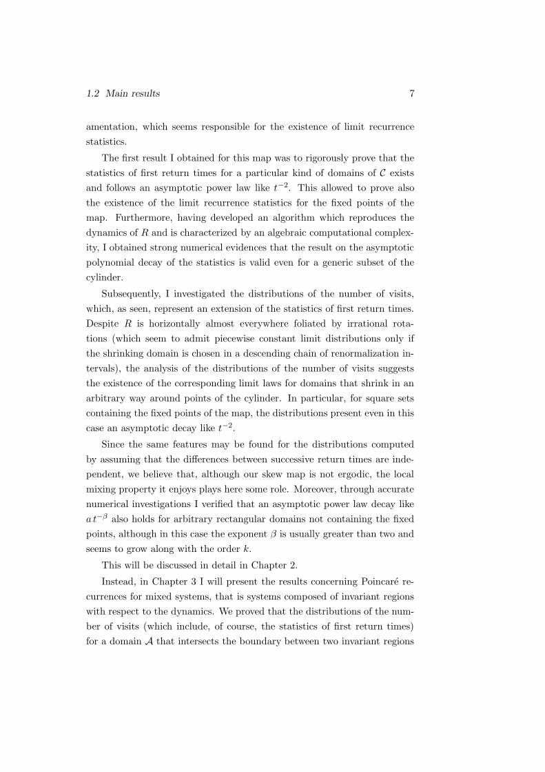
2.4 Distributions of the number of visits 23
10-8
10-6
10-4
10-2
100
10-1 100 101 102 103 104
F1(
t)
t
Figure 2.5: Distribution of the number of visits of order k = 1 computed
for the domain Aε = [0, ε]× [0, ε], with ε = 10−2. The dotted line represents
the function (2.22).
Numerical analysis
We compared the distributions Fk(t), computed under the assumption that
the differences of successive return times are asymptotically independent,
with the ones obtained through numerical investigations.
The qualitative features described above still seem to persist, although
there is some discrepancy between the two kind of distribution. In particular,
both show an initial plateau, even if the value of the actual one differs from
the expected. But, what is more interesting, all the numerical distributions
appear to decay like 1/2 t−2, at least after a transitory peak (see Figs. 2.5
and 2.6).
The discrepancy between the two kind of distribution is reasonably due
to the presence of some sort of weak correlation between the differences of
successive returns. Note that this could be in agreement with a result of
Z. Coelho and E. De Faria [24], showing that the limit joint distributions of
the differences of successive entry times are not given by the product of the
individual limit distributions.
I investigated also the behaviour of the distributions of the number of

24 Shear flow
10-8
10-6
10-4
10-2
100
10-1 100 101 102 103 104
F2(
t)
t
Figure 2.6: Distribution of the number of visits of order k = 2 computed
for the domain Aε = [0, ε]×[0, ε], with ε = 10−2. The dashed line represents
the function 1/2 t−2.
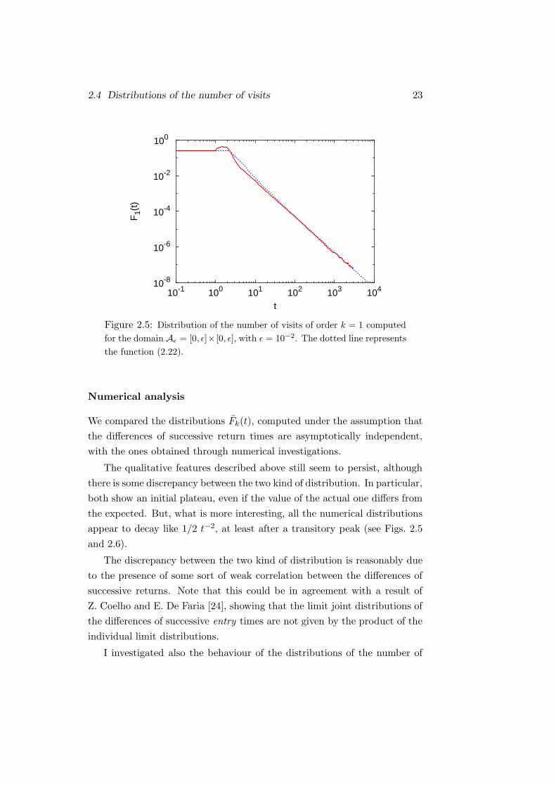
visits Fk,A(t) with A = [0, ε]×[y0, y0+ε] ⊂ C, y0 > 0, for several values of the
parameters y0 and ε. I found that an asymptotic power law decay preceded
by a peak seems to hold even for such domains, as shown in Fig. 2.7; note
how the peaks narrow and shift toward larger t when k increases, while their
height slightly decreases. So, in order to estimate the decay exponent β, I
used a least-squares method to fit the numerical distributions against the
function a t−β. In this more general case β is usually greater than 2, and
the mean value of its distribution appears to be positively correlated to the
order k (Fig. 2.8).
Even the distributions obtained for rectangular domains like A = [x0, x0+
ε] × [y0, y0 + δ] present similar features: in particular they decay following
a power law with an exponent greater, but near, to 2. Moreover, the mean
return time computed numerically is still 〈τA〉 = 1/ε.
In conclusion, the inverse square decay in t of the limit distributions,
whatever the order k, seems to be typical for the fixed points (which lie
along the x axis) of our skew map, while as soon as one considers other
points, the exponent β increases weakly with k. However, the difference
between the distributions of the number of visits for periodic and generic
2.4 Distributions of the number of visits 25
10-6
10-4
10-2
100
100 101 102 103
Fk(
t)
t
1 2 5 10 20
Figure 2.7: Distributions of the number of visits of order k = 1, 2, 5, 10
and 20, computed for the domain A = [0, ε] × [y0, y0 + ε], with y0 = 0.35
and ε = 10−2. The dashed line represents the function 1/2 t−2.
points appears to be a general fact of recurrences, as we will also see in the
next chapters.

26 Shear flow
1.95
2.00
2.05
2.10
2.15
k = 1 k = 2 k = 3
β
Figure 2.8: Distributions of the best-fit parameter β, obtained through a
least-squares method in the range 30 ≤ t ≤ 100 from the distributions of the
number of visits of order k = 1, 2 and 3. For each order k, the distributions
of the number of visits have been computed for twenty domains of side
ε = 10−2. The arrows show the position of the mean value of β.

Chapter 3
Mixed dynamical systems
In this chapter I will consider the following situation. Suppose to take a
subdomain A of a measurable phase space Ω, which intersects two regions
of Ω that are invariant with respect to a transformation T acting on Ω. Upon
these two regions, the map T is defined so that it behaves in two different
ways, for example it may be mixing on one of the components and simply
ergodic (or not ergodic at all) on the other one.
In this case, one could wonder about the existence of a limit recurrence
statistics — or, more generally, of limit distributions of the number of visits
— when A shrinks around a point which belongs to the common boundary of
the two regions, in such a way to still intersect the two invariant components.
3.1 Distributions of the number of visits
Let us consider a measurable space Ω and a map T acting on it. Moreover,
be µ a T -invariant measure; note that it can be taken as a generic invariant
measure, not necessarily a Lebesgue measure. Suppose now that the dynam-
ical system (Ω, T, µ) is such that it splits into two subsystems (Ω1, T1, µ) and
(Ω2, T2, µ), where
Ω = Ω1 ∪ Ω2, µ(Ω1 ∩ Ω2) = 0. (3.1)
The maps T1 and T2, defined over Ω1 and Ω2 respectively, satisfy the fol-
lowing conditions:
T1 = T|Ω1\(Ω1∩Ω2), T2 = T|Ω2\(Ω1∩Ω2), (3.2)
27

28 Mixed dynamical systems
that is, they coincide with T except possibly on the zero measure boundary
Ω1 ∩ Ω2 of the invariant regions.
In order to study the behaviour of the distributions of the number of
visits for neighborhoods of points which belong to this common boundary,
let us take a neighborhood A of a point x ∈ Ω1 ∩ Ω2, such that µ(A) > 0.
Then, denote with A1 and A2 the two different components of A, that is,
A1 = A∩ Ω1 and A2 = A∩ Ω2; of course A = A1 ∪A2.
The sequence of domains A shrinking around x is chosen in such a way
that the relative weights
w1(A) =µ(A1)
µ(A), w2(A) =
µ(A2)
µ(A), (3.3)
have a finite limit when µ(A) → 0, namely we will assume that the following
limits exist and are different from zero,
w1 = limµ(A)→0
w1(A), w2 = limµ(A)→0
w2(A). (3.4)
It is easy to prove that the mean return time into A is related to those
in A1 and A2 as follows:
〈τA〉 = w1(A) 〈τA1〉 + w2(A) 〈τA2
〉. (3.5)
In fact, from the definition of mean return time and of conditional measure,
it holds that
〈τA〉 =
∫
AτA(x) dµA
=1
µ(A)
∫
AτA(x) dµ
=µ(A1)
µ(A)
∫
A1
τA1(x) dµA1
+µ(A2)
µ(A)
∫
A2
τA2(x) dµA2
= w1(A) 〈τA1〉 + w2(A) 〈τA2
〉.
Furthermore, by calling Fk,A1(t) and Fk,A2
(t) the distributions of the
number of visits in A1 and A2 respectively, it is possible to show that
Fk,A(t) = w1(A)Fk,A1(w′
1(A) t) + w2(A)Fk,A2(w′
2(A) t), (3.6)

3.2 Coupling of mixing maps 29
where
w′1(A) =
〈τA〉〈τA1
〉 , w′2(A) =
〈τA〉〈τA2
〉 . (3.7)
Then, assuming that the limits
Fk,1(t) = limµ(A)→0
Fk,A1(t), Fk,2(t) = lim
µ(A)→0Fk,A2
(t), (3.8)
and
w′1 = lim
µ(A)→0w′
1(A), w′2 = lim
µ(A)→0w′
2(A), (3.9)
are well defined, we proved the following theorem.
Proposition 3.1 Under the existence of the limits (3.4), (3.8) and (3.9),
the limit distributions of the number of visits, for points on the boundary
Ω1 ∩ Ω2, exist and are given by
Fk(t) = w1 Fk,1(w′1 t) + w2 Fk,2(w
′2 t), (k ≥ 0) (3.10)
at the points of continuity of both Fk,1 and Fk,2.
In other words, when the conditions of Proposition 3.1 are satisfied, the limit
distributions Fk(t) are a linear superposition of the limit distributions Fk,i
corresponding to the invariant components Ai of the shrinking neighborhood
A, weighted by the relative size of such components.
As an application of these results, I first studied a one-dimensional sys-
tem whose phase space is parted into two mixing invariant regions, and then
a more remarkable two-dimensional system obtained by coupling the skew
map (2.1) with the so-called Arnold’s “cat map”.
3.2 Coupling of mixing maps
In order to check Eq. (3.10), I considered the following one-dimensional,
sawtooth-like map defined over the interval Ω = [−1, 1],
T (x) =
T1(x), if − 1 ≤ x < 0,
T2(x), if 0 ≤ x ≤ 1,
(3.11)

30 Mixed dynamical systems
where
T1(x) =
−3x − 3, if − 1 ≤ x < − 23 ,
3x + 1, if − 23 ≤ x < −1
3 ,
−3x − 1, if − 13 ≤ x ≤ 0,
(3.12)
and
T2(x) =
3x, if 0 ≤ x < 13 ,
2 − 3x, if 13 ≤ x < 2
3 ,
3x − 2, if 23 ≤ x ≤ 1.
(3.13)
Note that the two subsets Ω1 = [−1, 0] and Ω2 = [0, 1] are invariant as
regards T1 and T2, respectively.
The map T is piecewise linear and preserves the Lebesgue measure.
Moreover, it is continuous except at the point x = 0, which is a periodic
point of period two for T1 and a fixed point for T2. Thus, whenever we take
a ball of radius ε around x = 0, the statistics of first returns on the left and
on the right of x will follow, respectively, those around a periodic point of
period 2 and a fixed point; in this situation, the limit statistics for ε → 0
will not follow the exponential 1-law e−t as for generic points. Instead, it is
possible to use a result due to M. Hirata [15], according to which for one-
dimensional Markov maps, like T1 and T2, the statistics of first return times
in a ball of radius ε around a periodic point x of period P is given, in the
limit ε → 0, by the following formula:
F (t) = ρx e−ρxt, (3.14)
where
ρx = 1 − eu(x) + u(T (x)) + ...+u(T P−1(x)). (3.15)
Here u(x) is the potential associated to the invariant Gibbs measure; in the
present case, in which µ is a Lebesgue measure, it holds that
u(x) = ln1
|T ′1|
= ln1
|T ′2|
= ln(1/3) (3.16)
and, therefore, ρx is 8/9 for T1 and 2/3 for T2, consistently with the fact
that, in general, we expect ρx to approach 1 for periodic points of increasing
period.

3.2 Coupling of mixing maps 31
-4
-3
-2
-1
0
0 2 4 6 8 10 12
log 1
0 F
(t)
t
Figure 3.1: Statistics of first return times FA(t) obtained for the set A =
[−10−3, 10−3]. The dashed line represents the law (3.17).
Then, by using Proposition 3.1, the limit statistics of first return times
in x = 0 reads as
F0(t) = w1 F0,1(w′1 t) + w2 F0,2(w
′2 t) (3.17)
= w18
9e−
8
9w′
1t + w22
3e−
2
3w′
2t.
Since the maps T1 and T2 are mixing, one may immediately see, thanks to
Kac’s theorem, that 〈τAi〉 = µ(Ωi)/µ(Ai), i = 1, 2. So, under the existence
of the limits (3.4) and (3.9), we have w′i = [µ(Ω)/µ(Ωi)]wi. The prescribed
choice of the set A as a symmetric interval around the boundary point x
thus implies w1 = w2 = 1/2 and w′1 = w′
2 = 1. Replacing these values into
Eq. (3.17) gives a result which is well confirmed by the numerical computa-
tions, as shown, for example, in Fig. 3.1.
A similar situation occurs if we want to apply Proposition 3.1 to compute
the distributions of the number of visits, of order k > 0, in x = 0. That
is, we need to know which are the distributions around periodic points. In
this respect, since the two mixing maps T1 and T2 are conjugated with a
Bernoulli shift on three symbols with equal weights, it is possible to use
a general formula recently proved by N. Haydn and S. Vaienti which gives
the limit distribution of order k for cylinders Cn around periodic points of

32 Mixed dynamical systems
100
10-1
10-2
10-3
10-4
10-5
10-6
0 5 10 15 20 25
Fk(
t)
t
1
2
Figure 3.2: Distributions of the number of visits of order k = 1
and 2, computed for the map given by Eq. (3.11) in the interval
A = [−ε, ε], with ε = 5 × 10⁻⁴. The dotted lines represent the
theoretical predictions; in particular the one for k = 1 corresponds
to formula (3.20).
period P ,
Fk(t) ≡ limn→∞
µCn
(
x ∈ Cn : ξCn(t;x) = k
)
= (1 − pP ) e−(1−pP )tk∑
j=0
(k
j
)pP (k−j) (1 − pP )2j
j!tj , (3.18)
where p = µ(Cn+1)/µ(Cn). Note that for k = 0 this formula coincides with
the one found by M. Hirata, since then it reads as
F0(t) = (1 − pP ) e−(1−pP ) t. (3.19)
I would like to note that the distributions (3.18) can be obtained, under the
assumption that the differences of successive return times are asymptotically
independent, by convoluting F0(t) according to the procedure described in
Sec. 2.4.2.
Considering, for example, a sequence of shrinking cylinders Cn centered
around the point x = 0 (so that w1 = w2 = 1/2 and, by Kac’s theorem,

3.3 Coupling of a regular and of a mixing map 33
w′1 = w′
2 = 1), the distribution of the number of visits for k = 1 should be
well described by the following function:
F1(t) =1
2e−(1−p2)t (1 − p2)
[p2 + (1 − p2)2 t
]+
+1
2e−(1−p)t (1 − p)
[p + (1 − p)2 t
], (3.20)
where p = 1/3 in the present case. As Fig. 3.2 shows, the agreement of
the numerically computed distributions with the theoretical expectations is
really good.
3.3 Coupling of a regular and of a mixing map
It is particularly interesting to study the behaviour of the distributions of
the number of visits for a dynamical system in which the dynamics of one of
the invariant regions is given by our skew map, while the other is a generic
strongly mixing map, like, for example, the hyperbolic automorphism of the
torus (also known as Arnold’s “cat map”).
So, following the notation introduced in Sec. 3.1, let us construct a trans-
formation T defined over the two-dimensional space Ω = Ω1 ∪ Ω2, with
Ω1 = T × [0, 1] and Ω2 = T × [−1, 0[. In this way Ω is obtained by gluing
together the cylinder Ω1 with the torus Ω2. Then, the map T1 = T|Ω1be
represented by our skew map, while T2 = T|Ω2by the hyperbolic automor-
phism:
T2 :
x′ = 2x + y mod 1,
y′ = (x + y mod 1) − 1.(3.21)
Like in the previous example, µ is taken as the usual Lebesgue measure.
3.3.1 Recurrences for domains of finite size
In order to investigate the distributions of the number of visits, let us start
by considering an arbitrary point x = (x, 0) along the boundary (y = 0)
of the two invariant subspaces Ω1 and Ω2. Then, let us take a measurable
neighborhood A of x, in such a way that w1(A) = λ, with 0 < λ < 1. Of
course, by definition, it follows immediately that w2(A) = 1 − λ. Since the
domain A intersects the boundary, the distributions Fk,A(t) are given by
Eq. (3.6).

34 Mixed dynamical systems
Now, being T1 the skew map, we may use Eq. (2.4) to express the mean
return time into A1 like 〈τA1〉 = µy(IA1
)/µ(A1). Similarly, since T2 is
a strongly mixing map, we may apply Kac’s theorem, obtaining 〈τA2〉 =
1/µ(A2). So, the quantities w′1(A) and w′
2(A) read as
w′1(A) = λ
[
1 +1
µy(IA1)
]
, (3.22)
and
w′2(A) = (1 + λ) [1 + µy(IA1
)] , (3.23)
respectively.
Although we do not exactly know the distributions of the number of
visits Fk,A1(t) for the skew map when A1 is arbitrarily chosen, nevertheless
we may still understand the asymptotic behaviour of the limit distributions.
In fact, it is sensible to suppose, at least for large values of the normalized
time t and if A is sufficiently small, that Fk,A1(t) ' a t−β, with β very near
to 2, for k = 0, and slightly greater than 2 for k > 0, while a is a constant
positive number. This assumption is strongly suggested by the numerical
computations presented in Chapter 2 and supported also by the heuristic
explanations discussed there. Moreover, since the cat map, which is an
Anosov diffeomorphism, enjoys the Poisson distribution if we take balls or
cylinders converging around µ-almost all points, it is reasonable to expect
that the distributions Fk,A2(t) will approach the function e−t tk/k! when
µ(A) 1. Thus, using Eq. (3.6), we can write for t sufficiently large,
Fk,A(t) =λa
[w′1(A) t]β
+ (1 − λ)[w′
2(A) t]k
k!e−w′
2(A) t, (β ' 2). (3.24)
I verified that this formula, despite the approximations employed in or-
der to obtain it, describes quite well the asymptotic behaviour of the dis-
tributions of the number of visits computed for domains that intersect the
boundary, as shown in Figs. 3.3 and 3.4.
Note in particular that a power law tail appears as soon as the first
term in Eq. (3.24) gives the main contribution. Furthermore, the value
of the normalized time t for which the polynomial decay begins to prevail
increases as the measure of A decreases (but is still different from zero).
This means that if we compute numerically the distributions of the number
3.3 Coupling of a regular and of a mixing map 35
-7
-6
-5
-4
-3
-2
-1
0
0 10 20 30 40 50
log 1
0 F
(t)
t
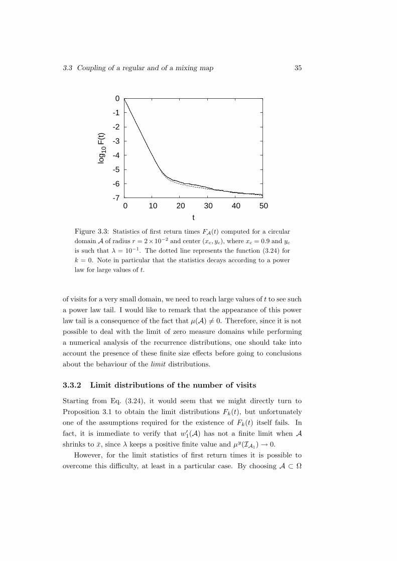
Figure 3.3: Statistics of first return times FA(t) computed for a circular
domain A of radius r = 2×10⁻² and center (xc, yc), where xc = 0.9 and yc
is such that λ = 10−1. The dotted line represents the function (3.24) for
k = 0. Note in particular that the statistics decays according to a power
law for large values of t.
of visits for a very small domain, we need to reach large values of t to see such
a power law tail. I would like to remark that the appearance of this power
law tail is a consequence of the fact that µ(A) 6= 0. Therefore, since it is not
possible to deal with the limit of zero measure domains while performing
a numerical analysis of the recurrence distributions, one should take into
account the presence of these finite size effects before going to conclusions
about the behaviour of the limit distributions.
3.3.2 Limit distributions of the number of visits
Starting from Eq. (3.24), it would seem that we might directly turn to
Proposition 3.1 to obtain the limit distributions Fk(t), but unfortunately
one of the assumptions required for the existence of Fk(t) itself fails. In
fact, it is immediate to verify that w′1(A) has not a finite limit when A
shrinks to x, since λ keeps a positive finite value and µy(IA1) → 0.
However, for the limit statistics of first return times it is possible to
overcome this difficulty, at least in a particular case. By choosing A ⊂ Ω
36 Mixed dynamical systems
10-8
10-6
10-4
10-2
100
100 101 102 103
F1(
t)
t
a
b
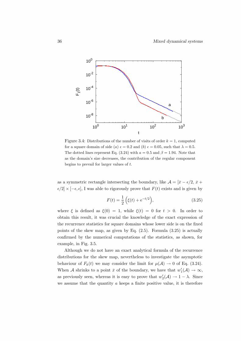
Figure 3.4: Distributions of the number of visits of order k = 1, computed
for a square domain of side (a) ε = 0.2 and (b) ε = 0.05, such that λ = 0.5.
The dotted lines represent Eq. (3.24) with a = 0.5 and β = 1.94. Note that
as the domain’s size decreases, the contribution of the regular component
begins to prevail for larger values of t.
as a symmetric rectangle intersecting the boundary, like A = [x − ε/2, x +
ε/2]× [−ε, ε], I was able to rigorously prove that F (t) exists and is given by
F (t) =1
2
(
ξ(t) + e−t/2)
, (3.25)
where ξ is defined as ξ(0) = 1, while ξ(t) = 0 for t > 0. In order to
obtain this result, it was crucial the knowledge of the exact expression of
the recurrence statistics for square domains whose lower side is on the fixed
points of the skew map, as given by Eq. (2.5). Formula (3.25) is actually
confirmed by the numerical computations of the statistics, as shown, for
example, in Fig. 3.5.
Although we do not have an exact analytical formula of the recurrence
distributions for the skew map, nevertheless to investigate the asymptotic
behaviour of Fk(t) we may consider the limit for µ(A) → 0 of Eq. (3.24).
When A shrinks to a point x of the boundary, we have that w ′1(A) → ∞,
as previously seen, whereas it is easy to prove that w ′2(A) → 1 − λ. Since
we assume that the quantity a keeps a finite positive value, it is therefore

3.3 Coupling of a regular and of a mixing map 37
-5
-4
-3
-2
-1
0
0 5 10 15 20
log 1
0 F
(t)
t
Figure 3.5: Statistics of first return times FA(t) computed for the set
A = [x, x + ε] × [−ε, ε], with x = 0.3 and ε = 10−2. The dashed line
represents the law (3.25).
immediate to verify that, for µ(A) → 0, only the second term survives in
Eq. (3.24), which thus becomes:
Fk(t) = (1 − λ)[(1 − λ)t]k
k!e−(1−λ) t. (3.26)
This result is actually confirmed by the numerical computations performed;
in particular, varying the fraction λ of the regular component of A, I checked
that the exponent is given by 1 − λ as expected (see Figs. 3.6 and 3.7).
Note that even if, in the limit of zero measure domains, the power law
contribution disappears from the distributions of the number of visits, which
thus follow, for sufficiently large t, a Poisson law as in the pure mixing case,
nevertheless the presence of the regular component of A is still revealed by
the fact that the quantity 1 − λ is different from one.
To conclude, the distributions of the number of visits appear able to
capture both the different qualitative properties of the regular and mixing
regions, and to provide some information about the relative measures of
these components.
As a final remark, I would like to stress that although the two-dimensional
model just considered is rather simple, the distributions of the number of

38 Mixed dynamical systems
-3
-2.5
-2
-1.5
-1
-0.5
0
0 1 2 3 4 5 6 7
log 1
0 F
(t)
t
1
2
3
45
Figure 3.6: Recurrence statistics FA(t) computed for circular domains Aof radius r = 10−2 and center (xc, yc), where xc = 0.9 and yc is such that
(1) λ = 0, (2) λ = 0.2, (3) λ = 0.4, (4) λ = 0.6 and (5) λ = 0.8.
visits exhibit some features that are found in dynamical systems having an
higher interest from a physical point of view, as we will see in the next
section.
3.4 Recurrences for the standard map
In this section I present the results obtained by investigating the distribu-
tions of the number of visits for the so-called “standard map,”
y′ = y − η2π sin(2πx)
x′ = x + y′mod 1. (3.27)
I chose the value of the coupling parameter as η = 3. In this way,
the phase space presents a structure where regular orbits are surrounded
by a chaotic “sea” (Fig. 3.8). Moreover, for such value of η the stochastic
layer, separating the regular orbits from the chaotic sea, is sufficiently sharp
compared to the size of the sets used to compute the distributions.
I considered three different cases: domains wholly contained in the regu-
lar region, domains lying on the chaotic sea, and domains that overlap both

3.4 Recurrences for the standard map 39
0
0.2
0.4
0.6
0.8
1
0 0.2 0.4 0.6 0.8 1
α(λ)
λ
Figure 3.7: Slopes α(λ) obtained by fitting the statistics of first return
times FA(t) against the function A e−α(λ) t, for 3 < t < 6. The domains
A are like the ones considered in Fig. 3.6. The dashed line represents the
function 1 − λ.
regions.
3.4.1 Domains on the regular region
The numerical distributions Fk,A(t) obtained for domains A wholly con-
tained in the regular region appear to follow asymptotically a power law
decay like a t−β, as shown in Fig. 3.9. The least-squares fit estimate of the
exponent β gives a value near 2, usually between 1.90 and 2.05. There is
furthermore some evidence suggesting that β slightly increases along with
the order k. It is interesting to note that the distributions computed for this
kind of sets behave in a very similar way as the ones got for the skew map.
3.4.2 Domains on the chaotic sea
The behaviour of the distributions of the number of visits for domains lying
on the chaotic component of the phase space appears, at first, surprising.

40 Mixed dynamical systems
0 0.30
0.3
x
y
Figure 3.8: Plot of the standard map (3.27) with coupling parameter
η = 3.
In fact, the computed mean return time is given, with a very good approx-
imation, by the ratio of the measure of the chaotic region (which is about
0.88 with the choice η = 3 for the coupling parameter) and the measure of
the considered domain, thus being in agreement with the value that would
be provided by Kac’s theorem (which holds for ergodic systems) if it could
be applicable here. On the other hand, for sufficiently large values of t the
distributions obtained reveal a departure from the expected Poisson law,
showing a polynomial decay with an exponent near 2 (see Fig. 3.10).
The reasons for such a rather unexpected feature could sensibly be due
to the fact that orbits originating even from points far away from the regular
region usually approach it. In this way, the overall chaotic motion would be
appreciably influenced by the regular component, leading to the appearance,
in the distributions of the number of visits, of the observed power law decay.
In this regard it is interesting to note that Poincare recurrences seem to
provide a tool capable to capture some of the properties of the dynamics in
a more “sensitive” way with respect to other quantities that could be used

3.4 Recurrences for the standard map 41
10-6
10-4
10-2
100
100 101 102 103
Fk(
t)
t
Figure 3.9: Distributions of the number of visits of order k = 1 (lower
curve), k = 2 (middle curve) and k = 3 (higher curve), computed for a
square domain of side ε = 2.5 × 10⁻² centered at (0.15, 0.25), which is
wholly contained in the regular region. The distributions appear to follow
asymptotically a power law decay like a t−β, where the least-square fit
estimate of β, performed for t in the range [10, 500], is 1.91 for k = 1, 1.95
for k = 2 and 1.97 for k = 3.
for the same purpose, like the mean return time into a given domain seen
above.
3.4.3 Domains intersecting the stochastic layer
Considering the results of Sec. 3.1, it is reasonable to expect that the asymp-
totic behaviour of the distributions of the number of visits for domains that
intersect the boundary between the regular and the chaotic regions should
be given by a linear superposition of a power law (the contribution, above
all, of the integrable orbits) and of a Poisson distribution (from the chaotic
sea).
In order to test this conjecture, I tried to fit the distributions Fk,A(t),
computed for a given domain A, against the following function, which should
sensibly represent their behaviour (from now on, to simplify the notation I
42 Mixed dynamical systems
10-8
10-6
10-4
10-2
100
100 101 102 103
Fk(
t)
t
12
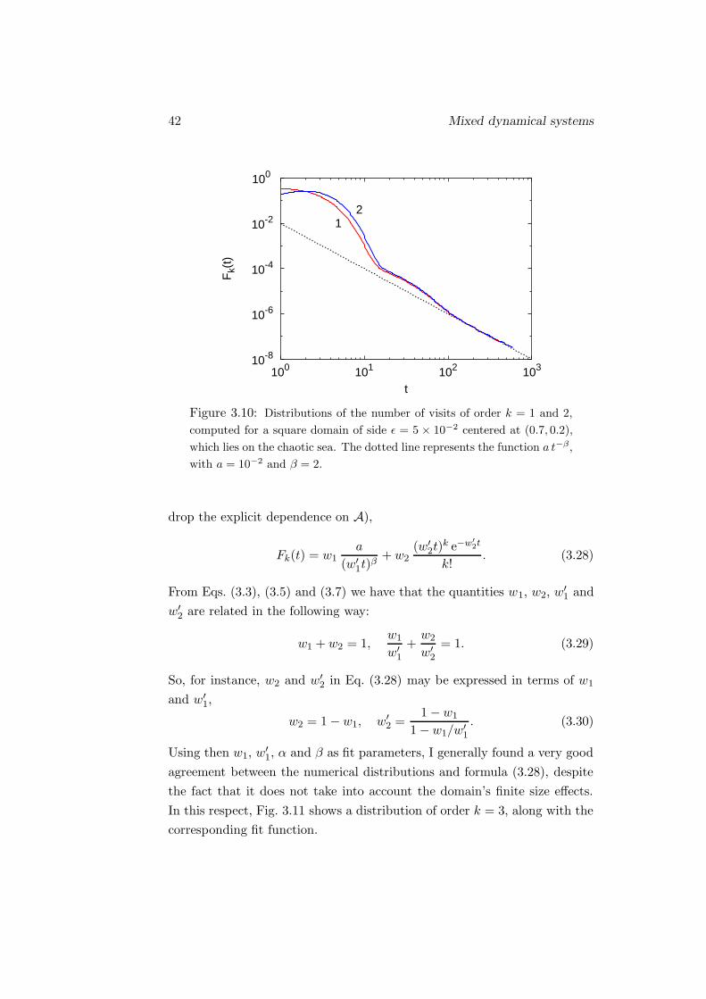
Figure 3.10: Distributions of the number of visits of order k = 1 and 2,
computed for a square domain of side ε = 5 × 10⁻² centered at (0.7, 0.2),
which lies on the chaotic sea. The dotted line represents the function a t−β,
with a = 10−2 and β = 2.
drop the explicit dependence on A),
Fk(t) = w1a
(w′1t)
β+ w2
(w′2t)
k e−w′2t
k!. (3.28)
From Eqs. (3.3), (3.5) and (3.7) we have that the quantities w1, w2, w′1 and
w′2 are related in the following way:
w1 + w2 = 1,w1
w′1
+w2
w′2
= 1. (3.29)
So, for instance, w2 and w′2 in Eq. (3.28) may be expressed in terms of w1
and w′1,
w2 = 1 − w1, w′2 =
1 − w1
1 − w1/w′1
. (3.30)
Using then w1, w′1, α and β as fit parameters, I generally found a very good
agreement between the numerical distributions and formula (3.28), despite
the fact that it does not take into account the domain’s finite size effects.
In this respect, Fig. 3.11 shows a distribution of order k = 3, along with the
corresponding fit function.

3.5 Dissipative Henon map 43
10-6
10-4
10-2
100
100 101 102 103
F3(
t)
t
Figure 3.11: Distribution of the number of visits of order k = 3 computed
for a square domain of side ε = 0.1 and centered at (0.03, 0.3), which
intersects the boundary between the regular and the chaotic regions. The
dotted line represents Eq. (3.28) with β = 2.04.
It is worthwhile to mention that, for a given domain A, usually the
value w1 obtained from the fit procedure is greater than the geometrical
estimate of the relative measure of the regular share of A. This discrepancy
seems reasonably due to the fact that besides the points belonging to the
regular share, which are responsible for the power law decay, there is a
further contribution from the chaotic component of A, whose dynamics is
influenced in some way by the regular orbits (as seen above), so that the
effective relative size of the regular component appears to be greater than
expected.
3.5 Dissipative Henon map
I would like to conclude this chapter by presenting some results, mainly
obtained by E. Lunedei [34], concerning the distributions of the number of
visits for generic and periodic points of the following map, that was intro-

44 Mixed dynamical systems
10-6
10-4
10-2
100
0 5 10 15
Fk(
t)
t
0
1
2
Figure 3.12: Distributions of the number of visits of order k = 0, 1 and 2,
computed for a circular domain of radius 5× 10⁻³ around a generic point.
The dotted lines represent the corresponding Poisson laws.
duced by Henon [35], defined on R2:
x′ = 1 + y − ax2,
y′ = bx,(3.31)
where a = 1.4 and b = 0.3.
In order to investigate the distributions of the number of visits Fk,A(t),
Lunedei used the so-called physical measure (also known as SBR measure)
supposing it is well defined, despite the fact that no rigorous proof about
its existence and its statistical properties has been given until now. The
numerical analysis was performed by taking the domain A as a little ball
centered both around generic and periodic points.
In the case of generic points, the distributions appear to agree in a very
good way with the Poisson law, as Fig. 3.12 shows. Since the Henon map is
not uniformly hyperbolic, we could not have taken for granted this result.
To study the distributions of the number of visits for periodic points he
computed, by a bisection method [36], the periodic orbits of the Henon map
with period P from one to ten. The investigation was limited up to points of
period ten because the lower periods are the ones with a stronger influence

3.5 Dissipative Henon map 45
10-8
10-6
10-4
10-2
100
0 2 4 6 8 10 12 14 16
F0(
t)
t
a
b
Figure 3.13: Distribution of the number of visits of order k = 0 computed
for a circular domain of radius 5 × 10⁻³ centered around a periodic point
of period two. The dotted line (a) corresponds to the exponential function
e−t, while the line (b) represents the function α e−αt, with α ' 0.66.
on return times. As expected, when A is a little ball centered around a
periodic point, the Poisson law does not fit anymore the numerical results,
as it is clear from Fig. 3.13, which shows the distribution F0,A(t) obtained
for a point of period two. Instead, for every periodic point considered, the
distributions of order k = 0 are well described by the function [compare it
to Eq. (3.19)],
F0(t) = α e−αt, (3.32)
where the coefficient α seems to depend on the period P in the following
way:
α(P ) = 1 − A%P , (3.33)
with A ' 0.96 and % ' 0.59 (see Fig. 3.14). Then, by making the assump-
tion of independence of the differences of successive return times, we used
a procedure similar to the one employed in Sec. 2.4.2 to obtain the limit
distributions of the number of visits of any order,
Fk(t) = α e−αtk∑
j=0
(k
j
)(1 − α)k−j α2j
j!tj. (3.34)

46 Mixed dynamical systems
0.4
0.5
0.6
0.7
0.8
0.9
1.0
1.1
0 2 4 6 8 10 12
α(P
)
P
Figure 3.14: Values of the coefficient α of the distributions F0(t) com-
puted for periodic points of period P . The dotted line represents the fit
function (3.33).
As Fig. 3.15 shows, the numerical distributions computed for periodic points
agree very well with this expression, which, under the identification α →(1 − pP ), coincides exactly with Eq. (3.18); like in that case, it would be
interesting here to explicitly relate α to the period. Moreover, we can note
that Eq. (3.34) is reduced to the Poisson function e−t tk/k! when α → 1.
Since α approaches 1 as the period increases, this means that the distribu-
tions for high periods are practically indistinguishable from those concerning
generic points, which are just described by the Poisson distribution. This
is self-consistent, because an aperiodic orbit can be thought like a periodic
orbit with an infinite period.
Summarizing this work on the Henon map, we may observe the following
facts. First, the distributions of the number of visits computed for generic
points agree with the Poisson law, as usually happens for systems with strong
mixing properties (see Ref. [8]). Second, periodic points exercise a real effect
on return times, and this effect decreases as the period grows. Furthermore,
the distributions computed for periodic points follow in a very good way the
behaviour predicted by assuming that the differences of successive return
times are independent.
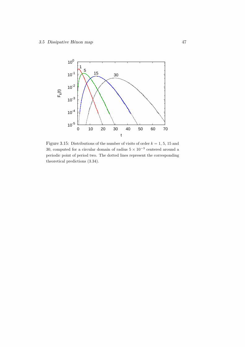
3.5 Dissipative Henon map 47
10-5
10-4
10-3
10-2
10-1
100
0 10 20 30 40 50 60 70
Fk(
t)
t
15
15 30
Figure 3.15: Distributions of the number of visits of order k = 1, 5, 15 and
30, computed for a circular domain of radius 5 × 10⁻³ centered around a
periodic point of period two. The dotted lines represent the corresponding
theoretical predictions (3.34).

48 Mixed dynamical systems

Chapter 4
Poincare recurrences and genomic
sequences
During the last years, we have assisted to a growing development of disci-
plines related to biology. In particular, the studies addressed to the inves-
tigation of genomes have attracted more and more attention. Surely, this
has been favoured, among other things, by the availability and easy access
to huge archives of genomic sequences.
Interestingly, the role of a part of the genome — the so-called noncoding
regions — is still substantially unknown. Understanding the function of
such noncoding regions appears even more important considering that they
usually represent, for eukaryotes, the widest portion of the genome, and
this part is generally larger in organisms placed at higher positions in the
evolutionary scale. For instance, in humans more than 95% of the genome
is represented by noncoding sequences.
Recently, many studies have been performed on genomic sequences us-
ing statistical methods (see for example Refs. [37]–[41]). In this respect,
G. Turchetti and I thought it could have been of some interest to explore the
possibility to apply the techniques developed for the analysis of dynamical
systems by means of Poincare recurrences. This idea was based essentially
on the observation that Poincare recurrences seem able to capture some
of the fundamental features of the dynamics of the underlying systems, as
shown in the previous chapter. So, I tried to investigate whether the re-
currence statistics may represent a tool capable to distinguish the coding
regions from the noncoding ones.
49
50 Poincare recurrences and genomic sequences
Unfortunately, the statistics of first return times does not appear suitable
for this purpose. Nonetheless the results obtained supply some information
that could be meaningful, I believe, in the discussion about the statistical
properties of genomic sequences.
4.1 Genome and genetic information
The deoxyribonucleic acid (DNA) is a macromolecule composed of funda-
mental units called nucleotides. In each nucleotide there is a phosphate
group, a sugar, and one of the following four bases: adenine (A), guanine
(G), cytosine (C) and thymine (T).
Several nucleotides bind themselves to form a chain-like molecule known
as polymer, which tends to assume an helical shape. Two of these helices,
linked together by hydrogen bindings between complementary bases, form
the DNA molecule. Usually, each helix is said to be a DNA strand.
The biological role of such a DNA molecule is fundamental: it represents
the so-called genome which contains the hereditary information own by every
living being. Its size differs from species to species; in humans it is made of
about 3.2 billion nucleotides.
The concept of gene was introduced by Mendel during his studies on
heredity to indicate the basic unit responsible for the transmission of a
single hereditary character. Modern biochemistry has revealed that a gene
is a specific sequence of nucleotides whose main function is, most of times,
to hold the information needed in the building of proteins. These latter are
macromolecules composed of aminoacids, and are essential for most of the
cellular activities.
A sequence of nucleotides determines an aminoacidic sequence (that is a
protein) in the following way: to every combination of three nucleotides is
associated one among twenty different aminoacid, according to the so-called
genetic code. The regions of a gene that concur to the formation of a protein
are named coding sequences.
What is surprising, is that usually only a small fraction of the whole
genome of eukaryotes is coding. In human beings, for example, more than
95% of DNA is represented by noncoding sequences, whose meaning is still
today widely unknown.
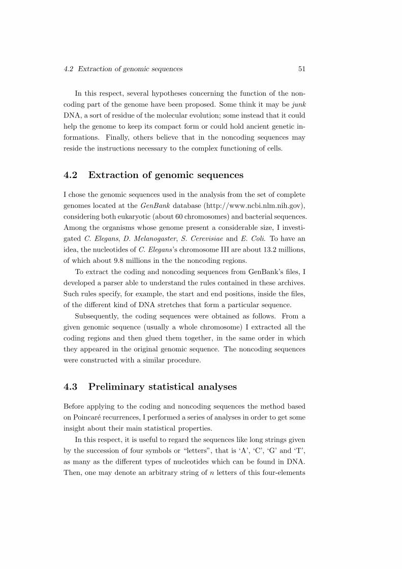
4.2 Extraction of genomic sequences 51
In this respect, several hypotheses concerning the function of the non-
coding part of the genome have been proposed. Some think it may be junk
DNA, a sort of residue of the molecular evolution; some instead that it could
help the genome to keep its compact form or could hold ancient genetic in-
formations. Finally, others believe that in the noncoding sequences may
reside the instructions necessary to the complex functioning of cells.
4.2 Extraction of genomic sequences
I chose the genomic sequences used in the analysis from the set of complete
genomes located at the GenBank database (http://www.ncbi.nlm.nih.gov),
considering both eukaryotic (about 60 chromosomes) and bacterial sequences.
Among the organisms whose genome present a considerable size, I investi-
gated C. Elegans, D. Melanogaster, S. Cerevisiae and E. Coli. To have an
idea, the nucleotides of C. Elegans’s chromosome III are about 13.2 millions,
of which about 9.8 millions in the the noncoding regions.
To extract the coding and noncoding sequences from GenBank’s files, I
developed a parser able to understand the rules contained in these archives.
Such rules specify, for example, the start and end positions, inside the files,
of the different kind of DNA stretches that form a particular sequence.
Subsequently, the coding sequences were obtained as follows. From a
given genomic sequence (usually a whole chromosome) I extracted all the
coding regions and then glued them together, in the same order in which
they appeared in the original genomic sequence. The noncoding sequences
were constructed with a similar procedure.
4.3 Preliminary statistical analyses
Before applying to the coding and noncoding sequences the method based
on Poincare recurrences, I performed a series of analyses in order to get some
insight about their main statistical properties.
In this respect, it is useful to regard the sequences like long strings given
by the succession of four symbols or “letters”, that is ‘A’, ‘C’, ‘G’ and ‘T’,
as many as the different types of nucleotides which can be found in DNA.
Then, one may denote an arbitrary string of n letters of this four-elements

52 Poincare recurrences and genomic sequences
0
0.05
0.1
0.15
0.2
0 0.2 0.4 0.6 0.8 1
f 2(x
)
x (word label)
actualproduct
Figure 4.1: Frequency distribution f2(x) of words two nucleotides long,
referring to the coding sequences from the chromosome III of C. Elegans.
alphabet with the term “word” (of length n). Of course, the total number
M of all the possible words of length n is M = 4n.
To each of these words it is possible to associate a number 0 ≤ x < 1, in
the following way. We can substitute the symbols ‘A’, ‘C’, ‘G’ and ‘T’ present
in given a word, with the digits 0, 1, 2 and 3, respectively. Thus, after such
a translation, a word may be reinterpreted as the base-four representation
of a whole number m. The number x associated to the word considered is
then simply obtained as x = m/M .
In this way, a sequence may be considered as the succession of contiguous
and non overlapping words of length n (each word, as said, representing a
group of n adjacent nucleotides in the sequence) or, equivalently, of points
belonging to the segment [0, 1[ whose coordinate is x.
4.3.1 Frequency distributions
In the beginning, I tried to analyze the presence of correlations among the
different types of letters (nucleotides), for both coding and noncoding se-
quences. For this purpose, I computed the normalized frequency distribu-
tion f1(x) of occurrence of single letters in a sequence, and the normalized
frequency distribution f2(x) of occurrence, in the same sequence, of two
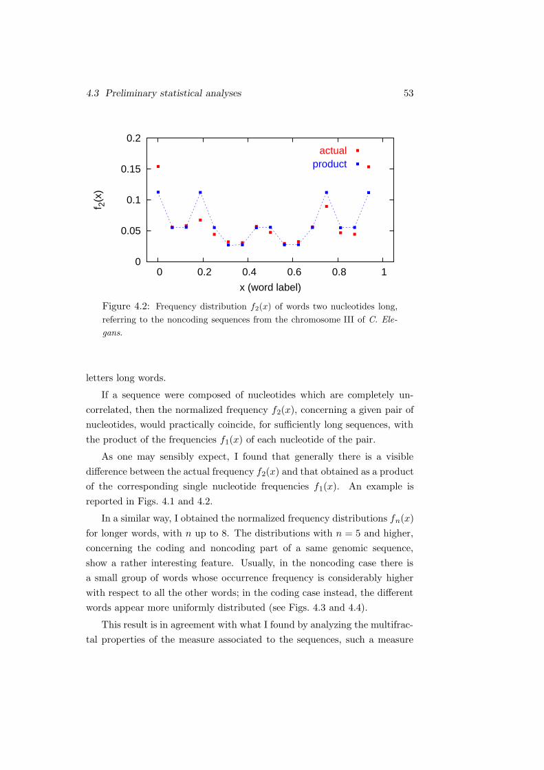
4.3 Preliminary statistical analyses 53
0
0.05
0.1
0.15
0.2
0 0.2 0.4 0.6 0.8 1
f 2(x
)
x (word label)
actualproduct
Figure 4.2: Frequency distribution f2(x) of words two nucleotides long,
referring to the noncoding sequences from the chromosome III of C. Ele-
gans.
letters long words.
If a sequence were composed of nucleotides which are completely un-
correlated, then the normalized frequency f2(x), concerning a given pair of
nucleotides, would practically coincide, for sufficiently long sequences, with
the product of the frequencies f1(x) of each nucleotide of the pair.
As one may sensibly expect, I found that generally there is a visible
difference between the actual frequency f2(x) and that obtained as a product
of the corresponding single nucleotide frequencies f1(x). An example is
reported in Figs. 4.1 and 4.2.
In a similar way, I obtained the normalized frequency distributions fn(x)
for longer words, with n up to 8. The distributions with n = 5 and higher,
concerning the coding and noncoding part of a same genomic sequence,
show a rather interesting feature. Usually, in the noncoding case there is
a small group of words whose occurrence frequency is considerably higher
with respect to all the other words; in the coding case instead, the different
words appear more uniformly distributed (see Figs. 4.3 and 4.4).
This result is in agreement with what I found by analyzing the multifrac-
tal properties of the measure associated to the sequences, such a measure
54 Poincare recurrences and genomic sequences
0
0.0005
0.001
0.0015
0.002
0.0025
0.003
0.0035
0 0.2 0.4 0.6 0.8 1
f 5(x
)
x (word label)
Figure 4.3: Frequency distribution f5(x) of words five nucleotides long,
referring to the coding sequences from the chromosome III of C. Elegans.
being constructed through the frequency distribution of occurrence of the
words.
4.3.2 Multifractal analysis
To perform the multifractal analysis of the coding and noncoding part of the
different genomic sequences, I considered uniform partitions of the segment
I = [0, 1). I recall that we are representing all the possible M = 22n words n
nucleotides long as points whose coordinate x is given by a number between
0 and 1, as explained above.
So, subdividing I into 2k subintervals Ij (1 ≤ j ≤ 2k), each subinterval
will contain 22n−k words, and it is possible to associate to each of them
a measure µ such that µ(Ij) is the sum of the normalized frequencies of
occurrence of the words belonging to Ij.
Now it is easy to compute the following quantity:
Nq(k) =
2k
∑
j=1
µ q(Ij), q ∈ R, (4.1)
where in the sum are considered only the subintervals Ij whose measure is
greater than zero. In order to obtain the multifractal spectrum f(α), we

4.3 Preliminary statistical analyses 55
0
0.005
0.01
0.015
0.02
0 0.2 0.4 0.6 0.8 1
f 5(x
)
x (word label)
Figure 4.4: Frequency distribution f5(x) of words five nucleotides long,
referring to the noncoding sequences from the chromosome III of C. Ele-
gans.
need to compute the function τ(q) that is defined as
τ(q) = limk→∞
−1
klog2 Nq(k). (4.2)
Of course, since the maximum order k which makes sense in the present case
is 2n, we can not deal with the limit operation in Eq. (4.2). Nonetheless, we
may obtain an estimate of τ(q) through a least-squares fit procedure; usually
the values get in this way are good for the analysis of sequences. Finally,
the multifractal spectrum is given by the Legendre transform of τ(q):
f(α) = minq
(αq − τ(q)). (4.3)
An important feature of the parabolic-shaped function f(α) is the following:
when the measure µ tends to be uniform, the corresponding f(α) is “nar-
row”, while it becomes “broader” as the measure gets more inhomogeneous.
Using the frequency of occurrence distributions fn(x), with n from 5 to
8, I found that the multifractal spectrum of the coding regions of a given
genomic sequence is usually narrower than that of the noncoding ones of the
same sequence, the difference being more evident for eukaryotic organisms.

56 Poincare recurrences and genomic sequences
-0.2
0
0.2
0.4
0.6
0.8
1
0.2 0.4 0.6 0.8 1 1.2 1.4 1.6 1.8
f(α)
α
codingnoncoding
Figure 4.5: Multifractal spectra of the coding and noncoding sequences
from the chromosome III of C. Elegans, obtained for words seven nu-
cleotides long.
This means that the coding part is composed of words more uniformly dis-
tributed, as suggested also by the functions fn(x) themselves. An example
of such a different behaviour is shown in Fig. 4.5, in which are reported
the multifractal spectra of the coding and noncoding regions concerning the
chromosome III of C. Elegans.
The results obtained could induce to think that if some information is
contained in the noncoding regions of the genome, then it may be coded
through a sort of “language”, meaning that there is a limited number of
words (representing the vocabulary of this language) which are used to con-
struct the “sentences” expressing such information.
To check this hypothesis I computed the Shannon entropy, which is pro-
portional to the compressibility degree (and thus to the informative content)
of a string, for the coding and noncoding sequences. Given an alphabet of
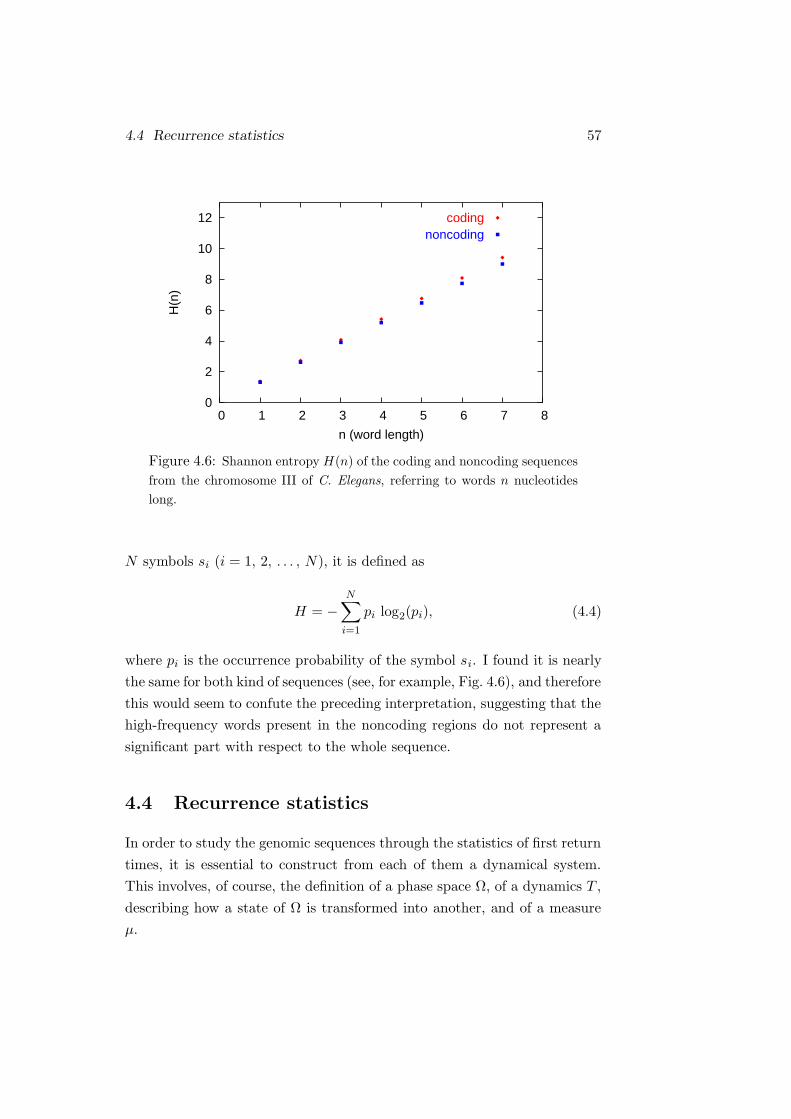
4.4 Recurrence statistics 57
0
2
4
6
8
10
12
0 1 2 3 4 5 6 7 8
H(n
)
n (word length)
codingnoncoding
Figure 4.6: Shannon entropy H(n) of the coding and noncoding sequences
from the chromosome III of C. Elegans, referring to words n nucleotides
long.
N symbols si (i = 1, 2, . . . , N), it is defined as
H = −N∑
i=1
pi log2(pi), (4.4)
where pi is the occurrence probability of the symbol si. I found it is nearly
the same for both kind of sequences (see, for example, Fig. 4.6), and therefore
this would seem to confute the preceding interpretation, suggesting that the
high-frequency words present in the noncoding regions do not represent a
significant part with respect to the whole sequence.
4.4 Recurrence statistics
In order to study the genomic sequences through the statistics of first return
times, it is essential to construct from each of them a dynamical system.
This involves, of course, the definition of a phase space Ω, of a dynamics T ,
describing how a state of Ω is transformed into another, and of a measure
µ.

58 Poincare recurrences and genomic sequences
-1.8
-1.6
-1.4
-1.2
-1
-0.8
-0.6
-0.4
-0.2
0
0 0.5 1 1.5 2 2.5 3 3.5 4
log 1
0 F
(t)
t
Y. Pestis CO92C. Elegans (III)
S. Cerevisiae (IV)D. Melanogaster (IV)
Figure 4.7: Statistics of return times referring to the coding sequences of
some organisms, for words seven nucleotides long. The dotted line repre-
sents the function e−t.
In this respect, many are the possible choices. Regarding the sequences
as given by the succession of words of length n, with n fixed, I decided to
consider the phase space Ω as the collection of all the possible words made
of n nucleotides. Then, I chose the dynamics T in such a way it associates
to a word x ∈ Ω, the word which immediately follows the first occurrence of
x in the sequence; if x does not occur in the sequence, it is simply ignored.
However, the sequences used are sufficiently long so that the words ignored
are generally very few, and therefore this does not constitute a problem at
all. I would like to remark that other definitions for the dynamics could
equally be considered. Finally, the measure µ of a subset A ⊆ Ω is given by
the ratio between the number of words belonging to A and the number of
those in the whole phase space.
Now, choosing two words x1 and x2, such that 0 ≤ x1 < x2 < 1, it is
possible to compute the recurrence statistics FA(t), with
A = x ∈ Ω : x1 ≤ x ≤ x2. (4.5)
The main result I obtained is that, regardless of the word’s length consid-

4.4 Recurrence statistics 59
-1.8
-1.6
-1.4
-1.2
-1
-0.8
-0.6
-0.4
-0.2
0
0 0.5 1 1.5 2 2.5 3 3.5 4
log 1
0 F
(t)
t
Y. Pestis CO92C. Elegans (III)
S. Cerevisiae (IV)D. Melanogaster (IV)
Figure 4.8: Statistics of return times referring to the noncoding sequences
of some organisms, for words seven nucleotides long. The dotted line rep-
resents the function e−t.
ered for the computation of the statistics of first return times, the recurrence
statistics is essentially the same for both kind of sequences. Moreover, FA(t)
seems to follow, with a very good accuracy, the exponential law:
fA(t) = exp
ln[1 − µ(A)] t
µ(A)
. (4.6)
Some of the statistics of first return times computed for words seven nu-
cleotides long in the coding and the noncoding case are reported in Figs. 4.7
and 4.8, respectively.
What appears surprising, is that a recurrence statistics as given by
Eq. (4.6) corresponds to a dynamical system whose dynamics loose “mem-
ory” of the past after one iteration only, and therefore this results suggests
that the words present in both kind of sequences are completely uncorre-
lated.
Thus, it seems sensible to conclude that, from the point of view of
Poincare recurrences, the coding and noncoding regions behave as they were
strongly mixing dynamical systems, which are characterized by a really rapid
decay of the correlations, and that the weight of the long-range correlations

60 Poincare recurrences and genomic sequences
is scarce, at least compared to the one concerning the short-range correla-
tions.

Bibliography
[1] H. Hu, A. Rampioni, L. Rossi, G. Turchetti and S. Vaienti, Statistics of
Poincare recurrences for maps with integrable and ergodic components,
Chaos 14, 160 (2004).
[2] L. Rossi and G. Turchetti, Poincare recurrences and multifractal prop-
erties of genomic sequences, Physica A 338, 267 (2004).
[3] L. Rossi, G. Turchetti and S. Vaienti, Poincare recurrences as a tool
to investigate the statistical properties of dynamical systems with inte-
grable and mixing components, J. Phys. Conf. Ser. 7, 94 (2005).
[4] N. Haydn, E. Lunedei, L. Rossi, G. Turchetti and S. Vaienti, Multiple
returns for some regular and mixing maps, Chaos 15, 033109 (2005).
[5] H. Poincare, Sur le probleme des trois corps et les equations de la
dynamique, Acta Math. 13, 1 (1890).
[6] J. D. Meiss, Symplectic maps, variational principles, and transport,
Rev. Mod. Phys. 64, 795 (1992).
[7] J. D. Meiss, Average exit times in volume preserving maps, Chaos 7,
139 (1997).
[8] M. Hirata, B. Saussol and S. Vaienti, Statistics of return times: a gen-
eral framework and new applications, Comm. Math. Phys. 206, 33
(1999).
[9] B. V. Chirikov and D. I. Shepelyansky, Asymptotic statistics of Poincare
recurrences in Hamiltonian systems with divided phase space, Phys.
Rev. Lett. 82, 528 (1999).
61

62 Bibliography
[10] G. M. Zaslavsky and M. K. Tippet, Connection between recurrence-
time statistics and anomalous transport, Phys. Rev. Lett. 67, 3251
(1991).
[11] G. M. Zaslavsky and M. Edelman, Weak mixing and anomalous kinetics
along filamented surfaces, Chaos 11, 295 (2001).
[12] S. Ornstein and B. Weiss, Entropy and data compression, IEEE Trans.
Inf. Theory 39, 78 (1993).
[13] V. Afraimovich, Pesin’s dimension for Poincare recurrences, Chaos 7,
12 (1997).
[14] B. Pitskel, Poisson law for Markov chains, Ergod. Theory Dyn. Syst. 11,
501 (1991).
[15] M. Hirata, Poisson law for Axiom-A diffeomorphisms, Ergod. Theory
Dyn. Syst. 13, 533 (1993).
[16] A. Galves and B. Schmitt, Inequalities for hitting time in mixing dy-
namical systems, Random Comput. Dyn. 5, 337 (1997).
[17] N. Haydn, Statistical properties of equilibrium states for rational maps,
Ergod. Theory Dyn. Syst. 20, 1371 (2000).
[18] M. Abadi, Exponential approximation for hitting times in mixing pro-
cesses, Math. Phys. Electron. J. 7, 2 (2001).
[19] M. Abadi and A. Galves, Inequalities for the occurrence times of rare
events in mixing processes. The state of the art, Markov Proc. Relat.
Fields 7, 97 (2001).
[20] H. Bruin and S. Vaienti, Return time statistics for unimodal maps,
Forum Math. 176, 77 (2003).
[21] N. Haydn and S. Vaienti, The limiting distribution and error terms for
return time of dynamical systems, Discrete Contin. Dyn. Syst. 3, 589
(2004).
[22] N. B. Slater, Gaps and steps for the sequence nθ mod 1, Proc. Cam-
bridge Phylos. Soc. 63, 1115 (1967).

Bibliography 63
[23] P. Alessandri and V. Berthe, Three distance theorems and combina-
torics of words, Enseignement Mathematique 44, 103 (1998).
[24] Z. Coelho and E. De Faria, Limit laws of entrance times for homeomor-
phisms of the circle, Isr. J. Math. 93, 93 (1996).
[25] N. Buric, A. Rampioni and G. Turchetti, Statistics of Poincare recur-
rences for a class of smooth circle maps, Chaos Solitons Fractals 23,
1829 (2005).
[26] Y. Lacroix, Possible limit laws for entrance times of an ergodic aperiodic
dynamical systems, Isr. J. Math. 132, 253 (2002).
[27] E. Floriani and R. Lima, Statistics of return times in a self-similar
model, Chaos 9, 715 (1999).
[28] V. Afraimovich and G. M. Zaslavsky, Fractal and multifractal prop-
erties of exit times and Poincare recurrences, Phys. Rev. E 55, 5418
(1997).
[29] V. Afraimovich and G. M. Zaslavsky, Sticky orbits of chaotic Hamilto-
nian dynamics, Lect. Notes Phys. 511, 59 (1998).
[30] V. Afraimovich, A. Maas and J. Urias, Symbolic dynamics for sticky
sets in Hamiltonian systems, Nonlinearity 13, 617 (2000).
[31] C. F. F. Karney, Long-time correlations in the stochastic regime, Phys-
ica D 8, 360 (1983).
[32] S. Tabachnikov, Billiards, Panoramas et Synthese (Society of Math.
Paris, France, 1995), Vol. 1.
[33] N. Haydn, Y. Lacroix and S. Vaienti, Hitting and return times in ergodic
dynamical systems, Ann. Prob. 5, 2043 (2005).
[34] E. Lunedei, Ricorrenze di Poincare in sistemi dinamici a bassa dimen-
sionalita, Ph.D. thesis, University of Bologna, Bologna, Italy, 2006.
[35] M. Henon, A two-dimensional mapping with a strange attractor, Com-
mun. Math. Phys. 50, 69 (1976).

64 Bibliography
[36] C. Polymilis, G. Servizi, Ch. Skokos, G. Turchetti and M. N. Vrahatis,
Local analysis of area preserving maps by topological degree theory,
Chaos 13, 94 (2003).
[37] R. N. Mantegna, S. V. Buldyrev, A. L. Goldberger, S. Havlin, C.-K.
Peng, M. Simons and H. E. Stanley, Systematic analysis of coding and
noncoding DNA sequences using methods of statistical linguistics, Phys.
Rev. E 52, 2939 (1995).
[38] A. Provata and Y. Almirantis, Scaling properties of coding and non-
coding DNA sequences, Physica A 247, 482 (1997).
[39] L. Luo, W. Lee, L. Jia, F. Ji and L. Tsai, Statistical correlation of
nucleotides in a DNA sequence, Phys. Rev. E 58, 861 (1998).
[40] H. E. Stanley, S. V. Buldyrev, A. L. Goldberger, S. Havlin, C.-K. Peng
and M. Simons, Scaling features of noncoding DNA, Physica A 273, 1
(1999).
[41] A. Som, S. Chattopadhyay, J. Chakrabarti and D. Bandyopadhyay,
Codon distribution in DNA, Phys. Rev. E 63, 051908 (2001).


