1
UNIVERSITY OF CALGARY
Numerical Modeling of Pipe-Soil Interaction
under Transverse Direction
by
Bahar Farhadi Hikooei
A THESIS
SUBMITTED TO THE FACULTY OF GRADUATE STUDIES
IN PARTIAL FULFILMENT OF THE REQUIREMENTS FOR THE
DEGREE OF MASTER OF ENGINEERING
DEPARTMENT OF CIVIL ENGINEERING
CALGARY, ALBERTA
AUGUST, 2013
©Bahar Farhadi Hikooei 2013

ii
Abstract
Based on Winkler method, pipe can be simplified as a beam, while pipe-soil interaction
can be represented by soil springs in the axial, horizontal and vertical direction. Pipe
deflection and resultant forces are related to each other by coefficient K in the equation
F=Kδ, where F is the resultant force and δ is the pipe displacement. This project studies
pipe-soil interaction for pipelines buried in clay and sand subjected to pipeline
displacement in oblique direction. The objective is to quantify the effect of soil
parameters on coefficient K and maximum soil resistance. Pipe-soil behavior has been
studied using the finite element software ABAQUS/CAE. There were totally 48 models
with varying soil parameters, pipe burial depth and pipe-soil interaction friction to
investigate the effect of each variable on pipe-soil behavior. The results have been
presented in normalized force-displacement plots to identify the parameters which
affect the soil resistance most. In addition they have been compared to the analytical
results from ALA (2001) and proposed failure envelopes in previous studies. The
results show that the maximum normal force per unit length depends on the type of soil
surrounding the pipe. By comparing all the results pipe burial depth, soil cohesion,
friction and dilation angles were found to have a significant effect on pipe-soil
interaction and can considerably increase the maximum soil resistance.
iii
Acknowledgements
I wish to express my sincere thanks to my supervisor Dr. R.C. Wong for his guidance
throughout this research. I am really grateful to Dr. Wong for all his patience, guidance and
suggestions during my master program.
I would like to extend my appreciations to my professors at University of Calgary during
my master program. That was a great chance for me to attend their classes.
Finally, I would like to thank my husband who was always with me in all hard times, my
parents who always supported me by their words, I owe all my life to you, and my parents
in-law who were by me in my loneliness.
iv
Table of Contents
Abstract.....................................................................................................................................ii
Acknowledgements ................................................................................................................iii
Table of Contents.....................................................................................................................iv
List of Tables............................................................................................................................vi
List of Figures and Illustrations ..............................................................................................vii
Chapter 1: Introduction to Pipeline Modeling.................................................................... 1
1.1 Introduction..................................................................................................................... 1
1.2 Literature review............................................................................................................. 3
1.3 Winkler method.............................................................................................................. 6
1.4 ALA guideline................................................................................................................ 7
1.5 Failure criteria.............................................................................................................. 10
Chapter 2: Finite Element Modeling.................................................................................. 13
2.1 Numerical modeling procedure................................................................................ 13
2.2 Pipe modeling........................................................................................................... 15
2.3 Soil modeling............................................................................................................ 15
2.4 Interface.................................................................................................................... 16
2.5 Modeling steps.......................................................................................................... 17
2.6 Modeling cohesive materials (clay).......................................................................... 19
2.7 Modeling frictional material (sand).......................................................................... 19
Chapter 3: Results and Discussions.................................................................................... 25
3.1 Behavior in cohesive material (clay)........................................................................ 25
3.2 Behavior in frictional material (sand)....................................................................... 29
3.2.1 Effect of pipe burial depth............................................................................ 30
3.2.2 Effect of inclination angles........................................................................... 31
3.2.3 Effect of sand friction angle......................................................................... 33
3.2.4 Effect of sand dilation angle......................................................................... 35
3.2.5 Effect of pipe-soil friction angle................................................................... 37 .
3.2.6 Effect of in-situ stress coefficient................................................................. 37
3.2.7 Linear elastic case versus elasto-plastic case............................................... 38
v
3.2.8 Superimposition of effects............................................................................ 39
3.2.9 Yield surface and Failure envelope.............................................................. 40
3.3 Surface heave........................................................................................................... 43
Chapter 4: Conclusion......................................................................................................... 65
4.1 Conclusion................................................................................................................ 65
4.2 Recommendation for future studies.......................................................................... 66
References .............................................................................................................................. 67
Appendices A: Symbols ......................................................................................................... 69
Appendices B: Lateral Bearing Capacity Factor of Soil (ALA2001)................................... 71
vi
List of Tables
Table 1. Input parameters in modeled cases:…………….…………………………………….21
Table 2. Effect of pipe displacement angle (α) on clay maximum resistance (Cu=35 kPa,
H/D=3.03)……………………………………………………...………………………………45
Table 3. Comparison of vertical and horizontal bearing capacity factors estimated from ALA
(2001) and finite Element modeling (Cu=45 kPa, H/D=3.03, α=0°)………………...…..…….45
Table 4.Comparison of vertical and horizontal soil resistance estimated from ALA(2001) and
finite element modeling (Cu=45 kPa, H/D=3.03, α=0°)………..……………….……….….….45
Table 5. Effect of pipe displacement angle (α) on sand maximum resistance (H/D=3.03, φ=35°
and Ψ=10°)…………..…………………………………………………………..………..……46
Table 6. Effect of friction angle on plastic deformation (H/D=3.03, Ψ=10°and α=0°)…..……46
Table 7.Maximum sand resistance for varying Ko (H/D=3.03, φ =35°, Ψ=10°, α=0°)…….…46
Table 8. Sand surface Heave for varying Ko (H/D=3.03, φ =35°, Ψ=10°, α=0°)…….....….…46
Table 9. Comparison between the effect of dilation angle and pipe displacement angle on
maximum resistance in sand for H/D=3.03 and φ =35°………………………………….….…47
Table 10. Comparison between the effect of friction angle and pipe burial depth on maximum
resistance in sand for pipe vertical displacement (α=0°) and Ψ=10°……………………..……47
Table 11.Comparing effect of different displacement angle on horizontal and vertical maximum
resistance in sand for H/D=3.03, φ =35° and Ψ=10°……………………....….……47
Table 12. Comparing the effect of different displacement angles and pipe burial ratio on
maximum resistance in sand for φ =35° and ψ =0° ……………………..….…………………47
Table 13.Comparing the effect of pipe-soil friction coefficient on maximum resistance in sand
for H/D=3.03, φ =35° and ψ=10°………………………………………..…..…………………48
Table 14.Comparision between bearing capacity factors and soil maximum resistance estimated
ALA(2001) and finite element modeling in sand………………………………………...……48
vii
List of Figures and Illustrations
Figure 1.Springs in BNWF model representing soil resistance (ALA, 2001) ............................................ 12
Figure 2 Schematic showing pipe-soil interaction, boundary conditions, and displacement angle ............ 23
Figure 3 Finite element mesh for pipe-soil interaction: a) Base model with 1996 elements for soil, and b)
Refined finite element mesh with 2453 elements for soil ........................................................................... 23
Figure 4 Mesh convergence study .............................................................................................................. 24
Figure 5 Dependency of force-displacement responses on pipe displacement angle for H/D=3.03, Cu=45
kPa, for total soil resistance, a) FEM results, and b) Guo (2005) ............................................................... 49
Figure 6 Dependency of force-displacement responses on pipe displacement angle for H/D=3.03, Cu=45
kPa, for the horizontal component of soil resistance a) FEM results, and b) Guo (2005) .......................... 50
Figure 7 Dependency of force-displacement responses on pipe displacement angle for H/D=3.03, Cu=45
kPa, for the vertical component of soil resistance a) FEM results, and b) Guo (2005) .............................. 51
Figure 8. Deformed finite element mesh as a result of pipe vertical displacement of δ/D=0.3, α=0⁰,
(Cu=45 kPa, H/D=3.03), Displacement contours (m) ................................................................................. 52
Figure 9. Deformed finite element mesh as a result of pipe oblique displacement of δ/D=0.3, α=45⁰,
(Cu=45 kPa, H/D=3.03), Displacement contours (m) ................................................................................. 52
Figure 10 Mobilization of vertical and horizontal resistances in clay for pipe displacement of δ/D=0.2 in
different displacement angles (α), H/D=3.03, Cu=35 kPa .......................................................................... 53
Figure 11. Normalized force-displacement curves for clay with different cohesion for H/D=3.03 and α=0
.................................................................................................................................................................... 53
Figure 12.Effect of pipe burial depth on force-displacement response in sand for φ=35°, Ψ=10°and α=0 54
Figure 13. Deformed finite element mesh as a result of pipe vertical displacement of δ/D=0.5, α=0°,
H/D=1.5, φ=35°, and Ψ=10°; Total displacement contours (m) ................................................................. 54
Figure 14. Deformed finite element mesh as a result of pipe vertical displacement of δ/D=0.5, α=0°,
H/D=6, φ=35°and Ψ=10°; Displacement contours (m) .............................................................................. 55
Figure 15. Deformed finite element mesh showing the plastic zone developed in sand as a result of pipe
vertical displacement of δ/D=0.5, H/D= 1.5, φ=35°and Ψ=10°. Plastic strain contours (%). ................... 55
Figure 16. Deformed finite element mesh showing the plastic zone developed in sand as a result of pipe
vertical displacement of δ/D=0.5, H/D= 6, φ=35°and Ψ=10°. Plastic strain contours (%) ........................ 56
Figure 17. Effect of pipe displacement angle on force-displacement response in sand for H/D=3.03,
φ=35°and Ψ=10° ......................................................................................................................................... 56
Figure 18. Effect of displacement angle on sand horizontal force-displacement response in sand for
H/D=3.03, φ=35°and Ψ=10° ....................................................................................................................... 57
Figure 19.Effect of loading angle on sand vertical force-displacement response in sand for H/D=3.03,
φ=35°and Ψ=10° ......................................................................................................................................... 57
Figure 20. Sand vertical resistances versus horizontal resistance, H/D=3.03, φ=35°, Ψ=10° .................... 58
Figure 21. Effect of friction angle on force-displacement response in sand for H/D=3.03, Ψ=10°and α=0°
.................................................................................................................................................................... 58
Figure 22. Effect of soil dilation angle on force-displacement response in sand for H/D=3.03, φ=35°and
α=0°............................................................................................................................................................. 59

viii
Figure 23. Effect of pipe-soil interface friction on force-displacement response in sand for H/D=3.03,
φ=35°, Ψ=10°and α=0° ............................................................................................................................... 59
Figure 24. Effect of Ko on sand force-displacement response, H/D=3.03, φ=35⁰, Ψ=20⁰, α=0⁰ ............... 60
Figure 25. Force-displacement response in elastic and elasto-plastic models, H/D=3.03, α=0° ................ 60
Figure 26. Failure envelope obtained from FEM analysis for different burial depth, compared to the
proposed model by Guo (2005a) for φ=35⁰, Ψ=10⁰ ................................................................................... 61
Figure 27. Failure envelope obtained from finite element normalized results for different burial depth,
compared to the proposed model by Guo (2005a) for φ=35⁰, Ψ=10⁰ ........................................................ 61
Figure 28. Yield surfaces obtained from FEM analysis for different loading surfaces, compared to the
proposed model by Guo (2005a), H/D=3.03, φ=35⁰, Ψ=10⁰ ..................................................................... 62
Figure 29. Effect of dilation angle and pipe burial depth on surface heave in sand for pipe vertical
displacement (α=0°) and φ= 35° ................................................................................................................. 62
Figure 30. Effect of dilation angle and pipe burial depth on surface heave in sand for pipe 45º
displacement (α=45°) and φ= 35° ............................................................................................................... 63
Figure 31.Effect of dilation angle and pipe burial depth on surface heave in sand for horizontal pipe
displacement (α=90°) and, φ= 35° .............................................................................................................. 63
Figure 32. Effect of dilation angle and pipe burial depth on surface horizontal displacement in sand for
pipe displacement of 45º (α=45°), and φ= 35° ............................................................................................ 63
Figure 33. Effect of dilation angle and pipe burial depth on surface horizontal displacement in sand for
pipe horizontal displacement (α=90°), and φ= 35° ..................................................................................... 63
1
Chapter One: Introduction to Pipeline Modeling
1.1 Introduction
Pipelines are safe and economical means of transporting gas, water, sewage and other
fluids. To provide a better protection and support, buried pipelines are used widely in
industry. Many of the existing pipelines are located at shallow depths beneath roads in
urban areas and are subjected to a variety of external loads. Failure of an oil and gas
pipeline can cause serious economic and environmental consequences, and in some
circumstances may lead to gas explosions resulting in loss of human life. Also, large
amount of money are being spent annually in repair and replacement of pipelines. In
terms of property damage PHMSA (Pipeline and Hazardous material safety
administration) records indicate that the 20-year average (1993-2012) cost of significant
pipeline incidents is over 318 million dollars, the 10-year average (2003-2012) cost is
over 494 million dollars, the 5-year average (2008-2012) cost is over 545 million dollars,
and the 3-year average (2010-2012) cost is over 662 million dollars.
In general, significant numbers of pipe damages are a result of induced loads in pipeline
that can happen as a consequence of permanent ground deformation, such as earthquakes,
slope failure, landslides and liquefaction.
Based on the annual report published by National Energy Board (NEB), 6% of the NEB-
regulated pipeline ruptures since 1991, due to geotechnical causes. (NEB, 2009)
To minimize the risk of any accident, injury and material loss and also to prevent the
damages that cause a great hazard to the environment, the pipeline industry has been
interested in predicting soil and pipe behavior when the pipeline is subjected to external
2
loadings. Owing to the highly nonlinear behavior of soil material, pipe-soil interface
phenomena, and the possibility of pipe distortion, buried pipe-soil system has a relatively
complex behavior.
3
1.2 Literature Review
Audibert & Nyman (1977) used an analytical method to determine the load-displacement
curve for buried pipes with different diameters. The analytical results were compared to
series of experiments on a small scale pipe model. Later, Nyman (1984) proposed an
analytical approach to accommodate the effect of oblique movement of pipes. Using the
similarity between the restraint of buried inclined anchor plates and restraint of pipelines
subjected to motion in the oblique direction, Nyman (1984) extended the behavior of soil
restraint in inclined anchors to buried pipes.
Based on Nyman’s equations (Nyman, 1984), the four principal directions of buried
pipeline restraint are vertical-uplift, horizontal-lateral, vertical-bearing, and longitudinal-
axial. The remaining soil restraint categories out-of-plane with the primary directions are
associated with oblique pipe motion. An analogy is made between restraint of buried
inclined anchor plates and restraint of pipelines subjected to motion in the horizontal-
vertical (lateral-uplift) direction. He proposed design procedures to develop bilinear load-
displacement relationship for soil restraint of pipelines subjected to oblique displacement.
Trautmann & O’Rourke (1985) studied the results of an experimental program to assess
the response of buried pipes to lateral ground movements considering the effect of pipe
depth, pipe diameter, and pipe roughness. A detailed research on buried pipeline
published by Guo & Stolle (2005a) studied the pipe-soil interaction for pipes buried in
frictional soil when subjected to lateral ground movement. In this study the effect of pipe
size and burial depth on pipe-soil peak strength was investigated by introducing a failure
surface in the force (or load) space to define the ultimate states of pipe–soil interaction.
The process of pipe movements is described by a set of loading surfaces and a plastic

4
displacement potential that defines the direction of incremental plastic pipe
displacements. The evolution of the loading surface, both the dimension and the shape,
depends on both pipe displacements and the burial depth ratio. Good agreement is
obtained between model predictions and the results of finite element analyses. The
proposed failure envelope has been discussed in section 1.5.
Following this study, Guo (2005b) published a study on the behavior of buried pipe in
clay under oblique loading. In this publication, the pipe-soil interaction for pipelines
subjected to combined horizontal and vertical movements in the oblique direction was
studied using finite element modeling. The study reproduced the key features of force-
displacement responses obtained from continuum finite element analyses for pipes of
different sizes and various burial depth ratios in clay. Another publication by Merifield et
al. (2008) focused on the results of finite element analyses of partially buried pipelines
under vertical and horizontal load. The results have been compared to the collapse loads
calculated using the upper-bound theorem of plasticity. In particular, these analyses
examine the influence of separation between the pipe and the soil when tension is
applied. Separate yield envelopes are derived for the cases involving separation (no
tension) and full bonding (full adhesion / unlimited
tension) at the pipe-soil interface.
Daiyan et al. (2010) studied the effect of displacement angle on the pipe-soil behavior in
the horizontal plane. In this experimental study the axial/lateral interaction of pipes in dry
sand has been investigated using a series of centrifuged tests of pipelines being displaced
5
in a horizontal plane. This experimental study shows that using discrete springs system in
structural modeling of pipe/soil interaction during axial/lateral pipe/soil movements
required coupled soil-spring formulations. Also, Badv & Daryani (2010) studied the
effect of pipe burial depth and pipe diameter on the upward and lateral soil-pipeline
interaction using finite difference method. Their study results showed that the transverse
soil restraint decreases for larger diameter pipes in the horizontal direction, and there is
no effect in the vertical direction. The transverse soil restraint increases with increasing
burial depth ratio but it becomes constant at deeper soil profiles.
With respect to the role of pipelines in industry and the importance of predicting pipeline
behavior, the American Lifelines Alliance (ALA) was formed with the purpose of
developing design provisions to evaluate the integrity of buried pipe for a range of
applied loads. According to ALA (2001) guideline, soil loading on the pipeline is
represented by discrete nonlinear springs (Winkler method), and several equations have
been proposed for the maximum soil resistance for buried pipeline in homogenous soil
condition. These expressions for the maximum soil spring force are based on laboratory
and field experimental investigations on pipeline responses, as well as general
geotechnical approaches for related structures, such as piles, embedded anchor plates, and
strip footings (ALA, 2001).
Another method used to predict the pipe-soil interaction behavior is the finite element
(FE) method, which provides a comprehensive tool for predicting the detailed
performance of buried structures. It can take into account the non-linear soil behavior,
bedding details, interaction between soil and pipe, and any geometric shape.
6
In this project the pipe-soil behavior under pipe displacement has been studied using
ALA equations, proposed failure criterion and finite element modeling.
The principal objectives of the present project are:
To study the interaction between pipe and soil under different oblique loading and
to identify the parameters that govern the interaction. By modeling pipe-soil
interaction using finite element method, the effect of soil parameters on the soil
maximum resistance and foundation coefficients in the Winkler model has been
studied.
To validate the existing predictive models developed by ALA (2001) and the
proposed failure criteria by Guo (2005). The pipe-soil behavior in different cases
has been compared to the force-displacement equations in ALA guidelines and
the proposed failure envelopes by varying pipe burial depth, soil cohesion, soil in-
situ stress coefficient, pipe-soil interface friction coefficient and soil dilation and
friction angles.
1.3 Winkler model
The beam on nonlinear Winkler foundation (BNWF), named as Winkler model is an
improved linear spring model and is used for predicting the nonlinear static response of
pipe-soil system. (Allotey & El Naggar, 2008)
In the Winkler model the soil-pipe interaction is modeled as a pipe resting on nonlinear
soil springs. In 2D modeling, the pipe can be modeled as a beam element and the soil
resistance along the pipe as nonlinear springs; there are four groups of springs to model
soil and pipe displacements and rotations:
7
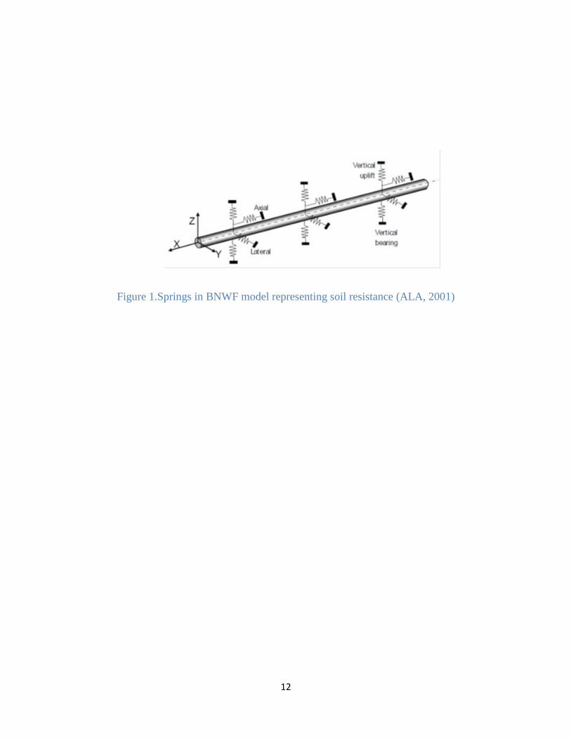
a) Axial soil spring: representing the soil resistance along the pipeline axis.
b) Lateral soil spring: representing the lateral resistance of soil to the pipe transverse
movement.
c, d) Vertical bearing spring and vertical uplift spring: representing the vertical resistance
of soil at the bottom and at the top of the pipe, respectively.
Figure 1 demonstrates these four groups of springs in Winkler method.
Based on Hooke’s law, a linear relationship between the force on the spring foundation
(F) and the deflection δ is assumed:
F=K.δ (1.1)
The modulus of subgrade reaction, K [F/L], is the ratio between the soil pressure per unit
length of pipe, P [F/L], and the displacement produced by the load application at that
point, δ.
In this project, since the 2D behavior of pipe-soil interaction has been modeled, the axial
soil spring is neglected and the modeling is based on the lateral springs and vertical uplift
and bearing springs.
1.4 ALA guideline
The limit theorems are powerful tools for analyzing stability problems in soil mechanics.
Limit analysis is a structural analysis field which is dedicated to the development of
efficient methods to directly determine estimates of the collapse load of a given structural
8
model without resorting to iterative or incremental analysis. The limit analysis is based
on two limit theorems: Lower and upper bound theorem:
In the lower bound theorem (Static Theorem) an external load computed on the basis of
an assumed distribution of internal forces, in which the forces are bounded by limit
values, and the forces are in equilibrium, is less than or equal to the true collapse load.
On the other hand in the upper bound theorem (Kinematic Theorem) an external load
computed on the basis of an assumed mechanism, in which the forces are in equilibrium,
is always greater than or equal to the true collapse load.
With respect to the limit analysis theorems, The American lifeline alliance (ALA)
guideline suggests the following equations to estimate the maximum lateral resistance of
soil per unit length of pipe:
(1.2)
where Cu is soil cohesion, D is the pipe diameter, H is the burial depth of the pipeline, and
is the effective unit weight of soil. Also, Nch and Nqh are the horizontal bearing capacity
factors for clay and sandy soils, respectively. They are given as:
( )
( ) (1.3)
(1.4)
where, x is the pipe burial depth ratio, which is the ratio of depth of the pipeline to the
pipe diameter (
).
9
The values for a, b, c, d and e can be found in design guidelines tables based on friction
angle (ALA, 2001). The table for capacity factors is attached in Appendix A.
With respect to equations (1.2) to (1.4), in ALA guidelines, the soil maximum lateral
resistance is a function of soil friction angle, cohesion and unit weight and also it is
highly related to the pipe burial depth ratio (
).
Furthermore, the maximum soil resistance per unit length of the pipeline in the vertical
uplift can be calculated:
(1.5)
where: (
) (1.6)
(
) (1.7)
By factoring the depth ratio from the above equations
{
} (1.8)
With respect to the equations above, same as the lateral resistance, the soil resistance in
the vertical uplift is a function of friction angle, cohesion, and effective unit weight of
soil. Also, it is linearly related to the pipe burial depth ratio.
In these equations when the pipes locates on soil surface, x=0, the maximu lateral soil
resistance will only have an cohesive component and will become:
10
And the maximum vertical soil resistance will become zero.
1.5 Proposed failure criteria
Nyman (1982) proposed an analytical approach to study the effect of oblique pipe
movement on the vertical and horizontal resistance of the soil:
(
)
(1.9)
with Fuh0 and Fuv0 being the maximum horizontal and vertical forces corresponding to
purely horizontal and vertical (upward) pipe movements, respectively. Fh and Fv are the
maximum horizontal and vertical soil resistances for a given pipe displacement. These
maximum horizontal and vertical forces resulted from pipe purely horizontal or vertical
displacement, Fuh0 and Fuv0, have been referenced to as Pu and Qu in ALA guideline,
respectively.
Later, Guo (2005), by comparing the experimental data of Das (1985) and Meyerhof and
Hanna (1978), used a modified form of failure criterion for cohesive soil:
(
) (
) (1.10)
He normalized Fuh0 and Fuv0 by undrained shear strength of clay and pipe diameter:
and
, (1.11)
where with respect to equations (1.2) and (1.5), Nch0 and Nch0 are the horizontal and
vertical bearing capacity factors for clay, respectively. For normalizing Fh0 and Fv0 in
sand, using equations (1.2) and (1.5), we can write:
11
and
. (1.12)
Furthermore, Guo (2005a) assumed the yield surface under induced oblique loading to
have the same functional form as the failure envelope:
(
)
(1.13)
Where the coefficient β is:
(1.14)
where Fho and Fvo are the horizontal and the vertical forces when the pipe undergoes
purely horizontal and vertical movement at a given pipe displacement, respectively.
(Note that Fuho and Fuvo are the maximum forces in the horizontal and vertical directions,
respectively.)
In this project the application of this failure criterion for sand has been studied. Also, the
results from finite element have been compared to those estimated from ALA (2001).
To distinguish between the results from different methods and avoid confusion, in this
project the horizontal and the vertical bearing capacity factors calculated from ALA
(2001), equations (1.4) and (1.7), are symbolized by Nqh and Nqv, and the horizontal and
the vertical bearing capacity factors from finite element modeling are represented by,
and
.
12
Figure 1.Springs in BNWF model representing soil resistance (ALA, 2001)
13
Chapter Two: Finite Element Modeling
In modeling the pipe-soil interaction, a number of aspects need to be considered:
The mechanical behavior of pipeline
The behavior of the soil surrounding the pipeline
The interaction between the soil and the buried pipeline.
The geometry and orientation of the pipeline
Proper elements for modeling pipe, soil and interface condition
In this project, the soil-pipe behavior has been modeled with a 2D numerical model using
finite element software, ABAQUS.
2.1 Modeling procedure
For selecting an appropriate element type for pipe-soil model, several element parameters
should be considered:
Family (continuum, shell, beam, rigid elements,…)
Degrees of freedom (directly related to the element family)
Number of nodes
Formulation
Integration
A family of finite elements is the broadest category used to classify elements and an
example of commonly used element families are: continuum, shell, beam, rigid,
membrane and etc. Elements in the same family share many basic features. One of the
14
major distinctions between different element families is the geometry type that each
family assumes.
Among different element families that ABAQUS provides, continuum or solid elements
can model the widest variety of components. They simply model small blocks of material
in a component and because of their shape they can be connected to other elements on
any of their faces and they can be subjected to any loading.
Continuum elements can be used for both linear analysis and also for complex nonlinear
analysis, which includes contact, plasticity, and large deformations.
In finite element methods for each element, displacement, rotations, pressure and other
degrees of freedom are only calculated at the nodes of the element and they are
interpolated between nodes for any other point in the element. This interpolation order
depends on the number of nodes on that element.
The elements with nodes only at their corners, use linear or first-order interpolations in
each direction and are often called linear elements or first-order elements while elements
with mid-side nodes, use quadratic interpolation (second-order interpolation). Second-
order elements provide a higher accuracy than first-order elements.
Since first-order elements are stiff and have a small rate of convergence and for using
them a very fine mesh is needed, which is not beneficial, they should be avoided as much
as possible in stress analysis problems. Consequently second-order elements, which
capture stress concentration more effectively, are better choices for modeling geometric
features.
15
The ABAQUS element library includes linear and quadratic interpolation elements in
one, two and three dimensions in various shapes. Triangles and quadrilaterals are
available in two dimensions while tetrahedrals and hexahedrals (bricks) are provided in
three dimensions.
Triangular and tetrahedral elements are geometrically adaptable, especially for complex
shapes and they are appropriate for large deformation problems. Although the
quadrilaterals and hexahedra elements have a better convergence rate than triangles and
tetrahedrals, they will become less accurate when their initial shape is distorted while
second-order triangles and tetrahedrals are less sensitive to the initial element shape
comparing to other elements. Based on the above fact the second-order triangle has been
chosen for modeling soil. Based on these elements behavior, the soil and pipe are
modeled as a 2D plane strain model with triangular elements.
2.2 Pipe modeling
In this project, pipe has been discretized with a 6-node quadratic plane strain triangle
(CPE6). Pipe is considered as a solid steel pipe with an inner diameter of 0.95 m and
thickness of 0.05 m. Since the rigid pipe is stiffer than the surrounding soil, the plastic
behavior of pipe is not a matter of interest and the pipe has been modeled with a linear
elastic material behavior with Young’s modulus of 200 GPa and Poisson’s ratio of 0.3.
The steel density is assumed to be 7850 kg/m3.
2.3 Soil modeling
Soil was modeled by a 6-node modified quadratic plane strain triangle (CPE6M).
Modified triangular or tetrahedral elements with mid-side nodes use a modified second-

16
order interpolation and are often called modified elements or modified second-order
elements. The most important concern in pipe-soil interaction numerical modeling is the
simulation of the soil’s stress-strain behavior. In finite element modeling, an elasto-
plastic material law with Mohr-Coulomb failure criterion and a non-associated flow rule
were considered to describe the behavior of clay and medium dense fine sand.
Mohr-Coulomb plasticity includes a yield function, f, which governs the onset of plastic
behavior and the plastic potential function, g, which governs the plastic flow.
(2.1)
(2.2)
where is the soil shear strength, σ is the soil stress, C is the soil cohesion, φ is the soil
friction angle and ψ is the soil dilation angle. Material parameters used in the model are
given in Table.1.
2.4 Interfaces
Among varieties of contacts models available in ABAQUS, surface to surface
interaction has been used for modeling the interface between soil and pipe. Surface-to-
surface contact interactions describe contact between two deformable surfaces or
between a deformable surface and a rigid surface.
The interaction between pipe and soil surface consists of two force components. One is
perpendicular to the interaction surface, which is the normal behavior, and the other one,
tangent to the surface, which is the tangential behavior and consists of sliding between
two surfaces and possibly frictional shear stresses. While modeling clay, the pipe-soil
17
interaction is assumed to be an adhesive friction and no sliding occurs before the shear
stress on the surface reaches to its maximum shear stress. This is numerically achieved
by assuming a large friction coefficient in Coulomb friction model in the soil-pipe
interface. In general, the maximum shear stress τmax along the pipe-soil interface can be
assumed to be 1/2Cu, where Cu is the cohesion of the soil.
In sand the friction coefficient between soil and pipe has a small value. The skin friction
angle between soil and steel pipe is about 20-30 , that will give a friction coefficient
between 0.3 - 0.5. In this study sand-steel friction coefficient for the base model has
assumed to be about 0.44. (Canadian foundation engineering manual, 1992)
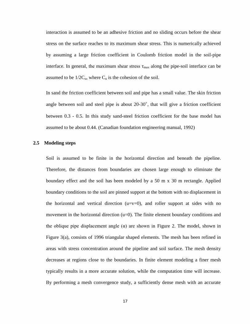
2.5 Modeling steps
Soil is assumed to be finite in the horizontal direction and beneath the pipeline.
Therefore, the distances from boundaries are chosen large enough to eliminate the
boundary effect and the soil has been modeled by a 50 m x 30 m rectangle. Applied
boundary conditions to the soil are pinned support at the bottom with no displacement in
the horizontal and vertical direction (u=v=0), and roller support at sides with no
movement in the horizontal direction (u=0). The finite element boundary conditions and
the oblique pipe displacement angle (α) are shown in Figure 2. The model, shown in
Figure 3(a), consists of 1996 triangular shaped elements. The mesh has been refined in
areas with stress concentration around the pipeline and soil surface. The mesh density
decreases at regions close to the boundaries. In finite element modeling a finer mesh
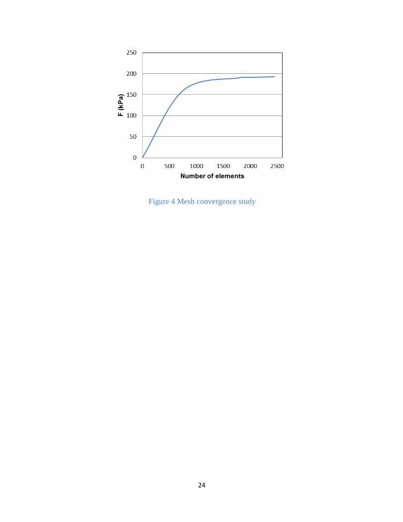
typically results in a more accurate solution, while the computation time will increase.
By performing a mesh convergence study, a sufficiently dense mesh with an accurate
18
solution can be obtained. To determine the most appropriate element number, other
models have been created in which the mesh has been refined by adding a denser mesh
at the top of the pipeline, using the biased meshing in soil surface. Figure 4 displays the
mesh convergence study. The models consist of 763, 1996 and 2453 elements,
respectively. Figure 3(b) displays a refined mesh model with 2453 elements as an
example. All three models have been subjected to a 0.5D pipe horizontal, vertical and
45° displacements. The difference between the soil maximum resistance between the
base model with 1996 elements and the model with 763 elements was about 12% and
the difference between the base model and the refined model with 2453 elements was
around 1%. As a result, since the base model is less time consuming and is as accurate
as the refined mesh, the first mesh has been chosen for this study.
The model has been created in three steps. In the initial step, the pipe and soil initial
conditions, like the boundary conditions and the interfaces between soil and pipe, has
been defined.
In the next step, a geostatic analysis is first performed to establish the initial stress state
in the soil. During this step, the gravity loads are applied and the pipe is allowed to
move without rotation. ABAQUS checks for equilibrium during this step using the
Mohr-Coulomb soil model to establish a stress field which balances the gravity load and
satisfies the boundary condition.
After the geostatic step, the loading step is applied in which the pipe displacement in a
given direction will be imposed to the pipe gradually.
19
2.6 Modeling cohesive material (clay)
To validate the models, buried pipeline in clay soil has been modeled under oblique
displacement, α, where α is the inclination angle of pipe movement with respect to the
vertical direction. Figure 2 presents the displacement angle, α. The model is a pipe in
clay where the clay has undrained shear strength of Cu= 45 kPa, and the pipe burial
depth ratio (H/D) is 3.03. (Undrained strength is typically defined by Tresca theory,
based on Mohr's circle as: σ1 - σ3 = 2 Cu , Where σ1 is the major principal stress and σ3
is the minor principal stress.)
The results have been validated by comparing them to the results in previous studies
(Guo, 2005a).
After validating the model, the effect of changes in the soil cohesion on Winkler
foundation modulus (K) has been plotted and also the maximum soil resistances in the
horizontal and vertical direction have been compared to the ALA soil resistance. The
results are discussed in Chapter 3.
2.7 Modeling frictional material (sand)
The next series of modeling is focused on the behavior of buried pipe in frictional
material. Based on the equations from ALA discussed above, there are several
parameters, such as pipe burial depth and soil friction angle that have high effect on soil
behavior. Also, there are some other parameters that have not been considered in ALA
equations, such as pipe-soil friction coefficient, soil dilation angle, and initial in-situ
stress. In this study the effect of these parameters on the soil-pipe behavior has been
studied. These behaviors have been modeled in 48 different cases, by varying
20
displacement angles (0°, 30°, 45°, 60°, and 90°), different pipe burial depth ratio (1.5, 3,
4.5, and 6), dilation angles (5°, 10°, 20°, and 30°) and also varying friction angles (25°,
30°, and 35°)
Three more cases have been selected to study the effect of friction coefficient on pipe-
soil interaction by varying the soil-pipe friction coefficient of 0.25, 0.44 and 0.8.
Also, the effect of initial in-situ stress on the pipe-soil behavior has been studied with
initial in-situ stress coefficients of 0.5, 0.75, and 1.
The results are discussed in two parts. In the first part, there will be a discussion about
the normalized force-displacement plots and maximum soil resistance in each case. In
the second part, there is a discussion on the effect of varying soil parameters on surface
heave.
The input parameters for each finite element model are summarized in Table 1.
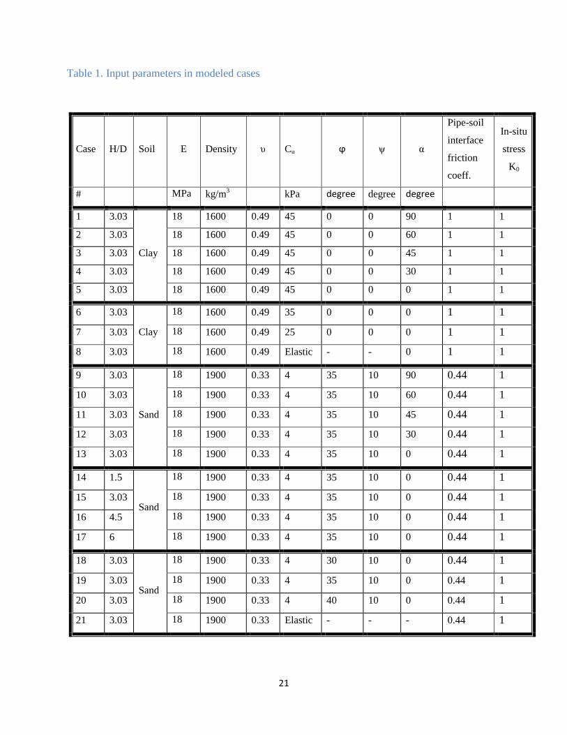
21
Table 1. Input parameters in modeled cases
Case H/D Soil E Density υ Cu ϕ ψ α
Pipe-soil
interface
friction
coeff.
In-situ
stress
K0
# MPa kg/m3 kPa degree degree degree
1 3.03
Clay
18 1600 0.49 45 0 0 90 1 1
2 3.03 18 1600 0.49 45 0 0 60 1 1
3 3.03 18 1600 0.49 45 0 0 45 1 1
4 3.03 18 1600 0.49 45 0 0 30 1 1
5 3.03 18 1600 0.49 45 0 0 0 1 1
6 3.03
Clay
18 1600 0.49 35 0 0 0 1 1
7 3.03 18 1600 0.49 25 0 0 0 1 1
8 3.03 18 1600 0.49 Elastic - - 0 1 1
9 3.03
Sand
18 1900 0.33 4 35 10 90 0.44 1
10 3.03 18 1900 0.33 4 35 10 60 0.44 1
11 3.03 18 1900 0.33 4 35 10 45 0.44 1
12 3.03 18 1900 0.33 4 35 10 30 0.44 1
13 3.03 18 1900 0.33 4 35 10 0 0.44 1
14 1.5
Sand
18 1900 0.33 4 35 10 0 0.44 1
15 3.03 18 1900 0.33 4 35 10 0 0.44 1
16 4.5 18 1900 0.33 4 35 10 0 0.44 1
17 6 18 1900 0.33 4 35 10 0 0.44 1
18 3.03
Sand
18 1900 0.33 4 30 10 0 0.44 1
19 3.03 18 1900 0.33 4 35 10 0 0.44 1
20 3.03 18 1900 0.33 4 40 10 0 0.44 1
21 3.03 18 1900 0.33 Elastic - - - 0.44 1

22
Case H/D Soil E Density υ Cu ϕ ψ α
Pipe-soil
friction
coefficient
In-situ
stress
K0
# MPa kg/m3 kPa degree degree degree -
22 3.03
Sand
18 1900 0.33 4 35 0 0 0.44 1
23 3.03 18 1900 0.33 4 35 5 0 0.44 1
24 3.03 18 1900 0.33 4 35 10 0 0.44 1
25 3.03 18 1900 0.33 4 35 20 0 0.44 1
26 3.03 18 1900 0.33 4 35 30 0 0.44 1
27 3.03
Sand
18 1900 0.33 4 35 10 0 0.25 1
28 3.03 18 1900 0.33 4 35 10 0 0.44 1
29 3.03 18 1900 0.33 4 35 10 0 0.8 1
30 3.03
Sand
18 1900 0.33 4 35 20 45 0.44 0.5
31 3.03 18 1900 0.33 4 35 20 45 0.44 0.75
32 3.03 18 1900 0.33 4 35 20 45 0.44 1
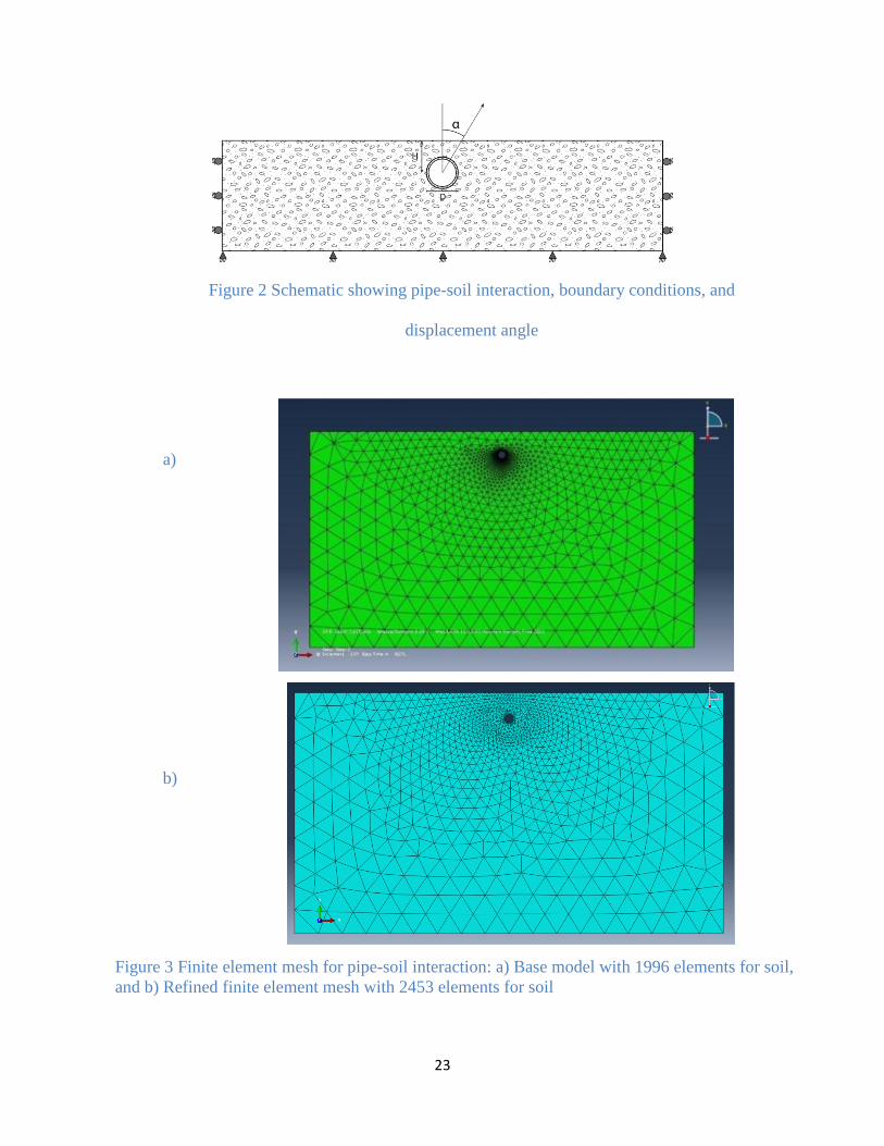
23
Figure 2 Schematic showing pipe-soil interaction, boundary conditions, and
displacement angle
a)
b)
Figure 3 Finite element mesh for pipe-soil interaction: a) Base model with 1996 elements for soil,
and b) Refined finite element mesh with 2453 elements for soil
24
Figure 4 Mesh convergence study
25
Chapter Three: Results and Discussions
In this chapter the results from finite element modeling has been compared to those
predicted by the ALA equations and the proposed failure criterion, using force-
displacement curves. In addition, the effect of soil parameters on pipe-soil interaction
has been studied using several cases with various soil parameters.
3.1 Behavior in cohesive material (clay)
As discussed before, to validate the model by comparing the results to those from the
previous studies (Guo, 2005), the buried pipe in clay has been modeled under varying
pipe displacement angles. In this model the burial depth ratio (H/D) is 3, with clay of Cu
= 45kPa and the pipe is subjected to different displacement angles (α). Using the finite
element results, the total resultant force and its horizontal and vertical components for a
given pipe displacement have been calculated and the relevant force-displacement
curves have been plotted. Figure 5(a) demonstrates the plot for the normalized total
induced force versus the normalized pipe displacement in various displacement
directions. Figure 6(a) shows the horizontal component of the induced force versus pipe
displacement in the horizontal direction. Figure 7(a) defines the plot for the vertical
component of the induced force versus the displacement in the vertical direction. Figures
5(b), 6(b), and 7(b) present the normalized force-displacement plots from Guo (2005),
where Nh and Nv are the normalized horizontal and vertical soil resistances for a given
displacement (Fh/CuD and Fv/CuD), respectively.
General agreement is achieved between the finite element results and those presented by
Guo (2005). The main difference between the plots is the slope in the elastic zone of the

26
model, which may be a result of differences in assumed Young modulus. This is due to
lack of information about the presumed Young modulus in Guo’s modeling.
Furthermore, there is a difference between the consequences of the soil resistances in
various pipe displacement between Figures 5(a) and 5(b). This difference rises from a
discrepancy between the discussion of the text and Figure 5(b) of Guo’s paper. As
discussed in his paper, the case with the pipe horizontal displacement (α=90°) should
have the highest soil resistance. However, the figure shows a different result, which may
be a misprint in the figure.
Based on Figures 5(a), 6(a) and 7(a), the elastic behavior of the pipe is limited to
relatively low load levels (F/CuD ≈ 2.0). Further loading produces a significantly non-
linear deformation. It is clear that by increasing the displacement angle, there will be an
increase in the maximum normalized horizontal force component and a decrease in the
maximum normalized vertical force component. The horizontal or vertical components
of the mobilized soil resistance in the oblique direction are smaller than that when the
pipe undergoes purely horizontal or vertical movement (α=90° and α=0°). Figures 8 and
9 display displacement contours for two cases: α=0° and α=45°. In the case of α= 45°,
the displacements in the vertical direction are higher than those in the horizontal
direction, which is due to the small vertical overburden that results in lower induced
forces in the vertical direction.
Figure 10 displays the vertical soil resistance versus the horizontal soil resistance in clay
with Cu = 35 kPa when subjected to a normalized δ/D of 0.2. Also, the yield surfaces for
δ/D of 0.01, 0.02 and 0.05 have been plotted using Fh0 of 107.4 kPa, 168.7 kPa,
211.8kPa, and Fv0 of 98.9kPa, 157.7 kPa, and 187.8 kPa, respectively. The calculated β
27
for each yield surface would be 1.08, 1.07 and 1.12. Also the failure surface has been
plotted using Fuh0 and Fuvo of 220.9 kPa and 191.6 kPa, respectively. Based on the plots,
in displacements smaller than δ/D=0.02, there is a linear relation between the soil
vertical and horizontal resistance components. Material yields and hardens as it passes
through states on successive yield curves. The mobilization of soil resistance can be
reflected by the evolution of yield surfaces with pipe displacements and the resistance
force will grow toward the maximum resistance force.
Table 2 gives the maximum soil resistance for different pipe displacement angles. Based
on the results, by increasing pipe displacement angles, the maximum soil resistance will
increase, and consequently the maximum soil resistance in the horizontal direction is
15% higher than the maximum soil resistance in the vertical direction.
Cohesion:
In natural soils, cohesion results from electrostatic bonds between clay particles and the
strength of a soil is a combination of the cohesive and frictional contributions. Thus by
increasing soil cohesion, the soil maximum resistance will increase.
To study the effect of soil cohesion on the pipe-soil interaction, three cases has been
model with different cohesion values of Cu=25, 35 and 45 kPa for a pipe burial depth
ratio (H/D) of 3.03. The force-displacement results for these cases have been plotted in
Figure 11. Also, an elastic case has been modeled to compare the elastic model to the
elasto-plastic model. In all these four cases, the pipe has been subjected to an upward
displacement (α=0).
28
Since the main objective of this section is to investigate the effect of soil cohesion on the
maximum soil resistance, the results in Figure 11 are displayed as total force versus
normalized displacement. Based on the results, soil with a higher cohesion, shows a
higher maximum soil resistance. The results indicate that by increasing soil cohesion
from 25 kPa to 35 kPa and then from 35 kPa to 45 kPa, the maximum soil resistance will
increase 26% and 21%, respectively. Tables 3 and 4 compare the results from finite
element modeling with those from ALA guideline. In Table 3, the ALA horizontal and
vertical upward soil bearing capacity factor, Nch and Ncv has been compared to the
horizontal and the vertical upward capacity factor, Fh/CuD and Fv/CuD from the finite
element analysis. According to the ALA (2001), Nch and Ncv are independent on soil
cohesions. Varying the soil cohesion will not affect their values, while the horizontal
and vertical upward bearing capacity factors from finite element modeling are highly
affected by the cohesion factor. Although they have been normalized by the cohesion
factor, the bearing capacity factor will decrease with increasing soil cohesion. For the
clay with cohesion of 25 kPa the ALA upward bearing capacity factor (Ncv) and the
upward bearing capacity factor calculated from finite element modeling (Fv/CuD), are
both 6.37. For clay with a larger cohesion, ALA predicts a lower upward capacity factor
than finite element modeling. Since the ALA has considered the soil cohesion effect on
the soil maximum resistance (Pu), and not the bearing capacity factor (Ncv), Table 4
compares the horizontal and upward maximum resistances from ALA (2001) and finite
element modeling.
With respect to Table 4, in both ALA and finite element modeling with increase in soil
cohesion, the maximum horizontal and vertical soil resistance (Fv and Fh) will increase,
29
which is a reasonable behavior based on the equations (1.2) and (1.5). The ALA (2001)
predicts the maximum vertical resistance (Qu) for soil with cohesion 25, 35 and 45 kPa
about 1%, 9% and 15% higher than the finite element modeling. On the other hand, for
the maximum horizontal resistance (Pu), the ALA (2001) gives a more conservative
value. For clay with 25 and 35 kPa cohesive strength the ALA horizontal maximum
resistances are 7% and 4 % lower than those from the finite element modeling.
Figure 11 compares the results from the elastic analysis and the elasto-plastic analysis.
All cases will follow the linear elastic behavior in pipe small displacement and the
induced force is proportional to the displacement. By increasing pipe displacement, in the
elasto-plastic cases the plastic deformation will be developed according to the yield and
plastic potential function, while in the elastic case the elastic deformation will grow
linearly. In the elastic model the soil resistance is overestimated, as a result of not
considering material plastic deformation.
3.2. Behavior in frictional material (sand)
To study the frictional material behavior, several pipe-sand cases have been modeled
with ABAQUS using modeling parameters shown in Table 1. The base case is a sand
model with a friction angle of 35⁰ and a dilation angle of 10⁰. Also, to avoid the model
convergence in the geostatic step, a small cohesion of 4 kPa has been assigned to the
sand model. Sand parameters have been varied to analyze the effect of each parameter
on the pipe-sand interaction behavior.
30
3.2.1. Effect of pipe burial depth
To design a buried pipeline, the minimum depth of soil cover that can provide sufficient
uplift resistance is a matter of concern. Since the capability of the soil to resist the
pipeline movement can affect the occurrence of upheaval buckling, pipeline burial depth
can highly affect the construction costs and it is important to find the safe and shallow
burial depth for the pipeline.
To find the most effective pipe burial depth, different values of burial depth, H, have
been modeled with a constant pipe diameter of 0.95 m. The modeled burial depth ratios
are: H/D=1.5, 3, 4.5 and 6. To study the effect of burial depth on the soil maximum
uplift resistance, the results are plotted as a normalized force-displacement graph for
each case, in Figure 12. The soil normalized maximum resistance per unit length of pipe
is highly affected by the pipe burial depth ratio (H/D) and by increasing the burial depth
ratio, the soil normalized maximum resistance increases. As observed in the curves for
the shallower pipelines the normalized maximum resistance develops at a small
displacement while for pipelines with a higher H/D, a larger pipe displacement is
required to mobilize the maximum soil resistance.
Figures 13 and 14 compare the surface heave using displacement contours for two cases
with H/D of 1.5 and 6 for the same amount of pipe displacement. Both cases have the
same soil parameters (E, υ, and ϕ,…) and only the pipe burial depth differs. Based on
these figures it is clear that the pipe with a lower H/D has a higher surface heave. For the
pipe with H/D of 6, the surface heave is less than half of the surface heave for the case
with H/D of 1.5. The surface heave will be discussed on section 3.3.

31
Furthermore, ABAQUS calculates the plastic strain by decomposing the total strain
values into the elastic and plastic strain components. The plastic strain is obtained by
subtracting the elastic strain from the value of total strain:
(3.1)
Figures 15 and 16 compare the plastic strain contours for pipelines with burial depth
ratios of 1.5 and 6, respectively. In the case with burial depth ratio of 6, the plastic zone
has not reached to the surface while for the case with depth ratio of 1.5 there is a small
plastic strain beneath the soil surface which will result in an earlier failure in smaller
burial depth.
3.2.2. Effect of pipe displacement angle
To study the effect of pipe displacement angle on the pipe-soil interaction, the pipe-
sand interaction has been modeled with different displacement angles, α. In all cases,
the burial depth ratio (H/D) is 3.03 with a sand friction angle of φ=35° and a dilation
angle of ψ=10°. Pipe displaces along different angles α of 0°, 30°, 45°, 60° and 90°,
with respect to the vertical direction.
Figure 17 compares the normalized force-displacement curves for different pipe
displacement angles when the pipe is subjected to a normalized displacement of
δ/D=0.4. Similar to the behavior in clay, the elastic response is limited to a very small
pipe displacement, and the plastic region will grow with a larger displacement. Also, by
increasing the displacement angle, the maximum soil resistance will increase. The
normalized horizontal and vertical force components versus the normalized horizontal
and vertical pipe displacement components have been plotted in Figures 18 and 19,

32
respectively. An increase in pipe displacement angle, α, will result in an increase in the
normalized maximum horizontal resistance, while by increasing the displacement
angle, the normalized maximum vertical soil resistance will decrease. Also, with an
increase of α, a smaller displacement is required to mobilize the maximum soil
horizontal resistance, while the maximum soil vertical resistance will develop at a
larger displacement.
Table 5 gives the maximum resistance force for different pipe displacement angles.
Based on the results in Table 5 and Figure 17, by increasing the pipe displacement
angle from the vertical direction (α=0⁰) to the horizontal direction (α=90⁰), the soil
maximum resistance will increase.
Figure 20 displays the vertical soil resistance component versus the horizontal soil
resistance component in sand when the pipe is subjected to a displacement of δ/D=0.3.
Also, the yield surfaces for δ/D of 0.01, 0.02, and 0.05 have been plotted using Fh0 of
89.5 kPa, 161.2 kPa, 292.3.8kPa, and Fv0 of 75.7 kPa, 104.7 kPa, and 149.1 kPa,
respectively. The calculated β for each yield surface would be 1.18, 1.54 and 1.96. Also
the failure surface has been plotted using Fuh0 and Fuvo of 313.6 kPa and 156 kPa,
respectively. In small pipe displacements less than δ/D=0.01, there is a linear relation
between the soil vertical and horizontal resistance components, while by increasing pipe
displacement, the material yields and hardens as it passes through the states on the
successive yield surfaces and the soil resistance will grow toward the maximum
resistance force. There is a general agreement between the proposed yield surfaces of
equation (1.13) and the results from the finite element modeling. While comparing the
FEM results with the proposed failure envelope of equation (1.10), the induced forces

33
plots do not reach to the proposed failure envelope and the proposed failure envelope
overestimates the induced forces at failure.
Furthermore, based on Figure 20, by increasing the pipe displacement, the rate of
increase in the soil maximum resistance in the vertical direction is smaller than that in
the horizontal direction.
3.2.3. Effect of sand friction angle
Based on equations (1.3) and (1.4), the coefficients a, b, c, d and e are highly affected
by the friction angle that can emphasize the high effect of friction angle on the
maximum soil horizontal resistance predicted by ALA (2001). Also, in ALA (2001)
equations the friction angle has a direct relationship with the maximum vertical
resistance of soil. To study these relations in sand, several cases have been modeled
using sands with friction angles of 30⁰, 35⁰ and 40⁰ and a constant dilation angle of
10⁰. In all these four cases the pipe burial depth ratio (H/D) is 3.03 and the pipeline has
been subjected to a vertical displacement (α=0⁰).
Figure 21 displays the normalized force-displacement plot for each case. Based on the
plots, an increase in the friction angle will result in an increase in the maximum soil
resistance and increase in the mobilized δ/D.
Based on Mohr-Coulomb yield function, the plastic failure develops if the shear stress
τn on a plane exceeds a constant fraction of the normal stress σn:
| | (3.2)
where tan(φ) is the coefficient of friction and C is soil cohesion.
34
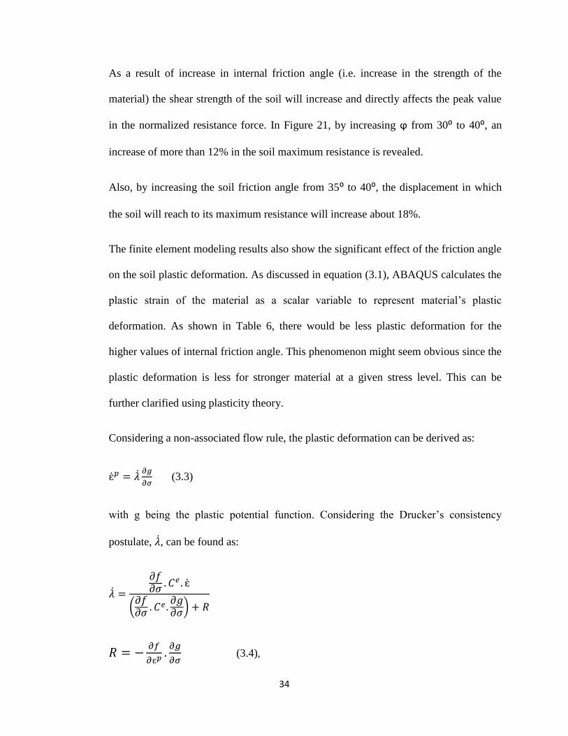
As a result of increase in internal friction angle (i.e. increase in the strength of the
material) the shear strength of the soil will increase and directly affects the peak value
in the normalized resistance force. In Figure 21, by increasing ϕ from 30⁰ to 40⁰, an
increase of more than 12% in the soil maximum resistance is revealed.
Also, by increasing the soil friction angle from 35⁰ to 40⁰, the displacement in which
the soil will reach to its maximum resistance will increase about 18%.
The finite element modeling results also show the significant effect of the friction angle
on the soil plastic deformation. As discussed in equation (3.1), ABAQUS calculates the
plastic strain of the material as a scalar variable to represent material’s plastic
deformation. As shown in Table 6, there would be less plastic deformation for the
higher values of internal friction angle. This phenomenon might seem obvious since the
plastic deformation is less for stronger material at a given stress level. This can be
further clarified using plasticity theory.
Considering a non-associated flow rule, the plastic deformation can be derived as:
(3.3)
with g being the plastic potential function. Considering the Drucker’s consistency
postulate, , can be found as:
(
)
(3.4),

35
where:
f: yield function
g: plastic potential function
: plastic multiplier
Ce: total Stress increment tensor
: total stress increment tensor
If we consider the normal forces, for example, the term
is equal to the mobilized
friction angle which is a direct function of the ultimate internal friction angle at failure.
If we assume that
, then the change in λ due to the change in mobilized
friction angle can be calculated as follows:
[(
) ]
(3.5)
Since R is a negative parameter in the equation above, we can imply that decreases
with increase in the mobilized friction angle; hence the plastic deformation decreases as
the friction angle increases.
3.2.4. Effect of sand dilation angle
Based on Taylor (1948) stress-dilatancy rule:
(
) (3.6)
36
The peak shear stress ratio (
) consists of components of interlocking (dy/dx),
which shows rate of dilation, and sliding friction between grains, μ. Therefore, the peak
shear stress ratio directly depends on the dilation angle.
In frictional soils the angle of dilation controls the amount of plastic strain developed
during shearing and it is assumed to be constant during plastic yielding.
(3.7)
It is obvious that for a dilation angle greater than zero the plastic volumetric strain rate
will be negative and therefore lead to dilation.
Besides, as discussed before, in the non-associated flow rule the plastic strain rates are
written as:
(3.8)
where is the plastic strain-rate, λ is a non-negative multiplier, σ is the Cauchy stress
tensor and g is the plastic potential function which depends on the stress and on the
instantaneous dilation angle ψ.
The effect of dilation angle has been studied using the base case, sand with friction
angle of 35⁰ and cohesion of 4 kPa with pipe burial depth ratio of 3.03, and varying
dilation angles of ψ= 0°, 5°, 10°, 20°, and 30⁰.
Based on the plotted results on Figure 22, by increasing the dilation angle, the soil
stiffness does not change significantly and the maximum resistance achieved will be
37
around the same displacement as it happens in other cases, which is about 0.05D. While
by increasing the dilation angle the maximum soil resistance will increase considerably.
3.2.5. Effect of pipe-soil friction coefficients
The effect of pipe and soil friction coefficient on pipe-soil interaction has been studied
with varying friction coefficients of 0.25, 0.44, and 0.8. In all cases the pipe burial depth
ratio (H/D) is 3.03, the friction angle is ϕ = 35⁰ and the dilation angle is Ψ=10 ⁰. The
pipe is subjected to a vertical displacement, α=0⁰.
Figure 23 indicates that the decrease in the soil-pipe interface friction does not
significantly affect the soil maximum resistance. Among these three cases, the case with
pipe-soil friction coefficient of 0.44 has the highest soil maximum resistance compared
to the other cases. The maximum soil resistance for this case is about 1% higher than the
other coefficient that is negligible.
Cases with a friction coefficient smaller than 0.2, will fail at the first step of loading
while subjecting to the pipe displacement.
3.2.6. Effect of in situ stress coefficient
The in situ stresses represent an important initial condition for geotechnical analysis. It
controls the distribution of stresses under soil surface. Typically, the horizontal stress is
computed from the vertical stress using the coefficient of earth pressure at rest, Ko,
which depends on micro-structure of the soil, geometry of the soil, stress history and
relative density of soil.
In this project, the effect of coefficient of earth pressure at-rest on the maximum soil
resistance has been verified by modeling three sand samples with the cohesion of 4 kPa,

38
the dilation angle of 20⁰ and H/D= 3.03, using different Ko of 0.5, 0.75, and 1 and pipe
displacement of α=45°.
Based on the results in Figure 24 and also Table 7, by increasing the coefficient of earth
pressure at-rest from 0.5 to 1, the soil maximum resistance increases about 1.5%.
Although the coefficient of earth pressure at-rest has a small effect on the soil
maximum resistance, it has a higher effect on the soil maximum horizontal resistance.
This is due to the dependency of the stress distribution to the coefficient of earth
pressure at-rest
Also, in Table 8 the surface heave results display that by increasing the coefficient of
earth pressure at-rest from 0.5 to 1, the surface heave will increase about 0.57%.
3.2.7. Linear elastic case versus elasto-plastic case.
Based on theory of plasticity, the strains and strain rates are decomposed into an elastic
part and a plastic part, where:
ε =εe+ε
p and έ=έ
e+έ
p
Figure 25 compares the force-displacement curve for an elastic case and a plastic case
with friction angle of 35⁰, dilation angle of 10⁰ and soil cohesion of 4 kPa. The pipe
burial depth ratio for both cases is H/D=3.03. The models behave the same up to the
yield point and then the plastic case behaves based on the assigned failure envelope.
Based on the plot, the elastic case overestimates the soil maximum resistance.
It is obvious that the linear elastic model is usually inappropriate to model the highly
non-linear behavior of soil, unless the modeling is for very small elastic displacements.

39
3.2.8. Superimposition of effects
Different cases with varying soil parameters were studied to define the effect of each
parameter on the soil maximum resistance and the surface heave. The effect of each
parameter on the surface heave will be discussed on section 3.3. The maximum soil
resistance from the finite element analysis for some parameters has been summarized in
Tables 9 to 13. Based on Table 9 with the pipe displacement in any direction, by
increasing the dilation angle, the soil maximum resistance will increase. Also, as the
pipe displacement goes from the vertical direction to the horizontal, soil will have a
higher total maximum resistance. In the vertical pipe displacement, by increasing soil
dilation angle from 0° to 20° the soil maximum resistance will increase 26%, while in
the horizontal pipe displacement, it will increase 33%.
In Table 10, the effect of the friction angle and pipe burial depth ratio on the soil
maximum resistance has been compared. An increase in the friction angle has a higher
effect on the maximum resistance of soil in deeper pipelines comparing to shallow
pipelines.
Table 11 compares the vertical and horizontal soil maximum resistance components for
different pipe displacement angles, α. Table 12 compares the effect of the pipe burial
ratio (H/D) on the soil maximum resistance, while the pipe is subjected to different
displacement angles. As discussed before by increasing the pipe burial ratio from 1.03 to
3.03, the soil maximum resistance will increase 230%, 250% and 300% for the
horizontal, 45º and the vertical pipe displacement, respectively.
40
Based on the previous discussions and Table 13 for a pipe-soil friction coefficient of
0.25, soil fails with very small displacement, and by increasing friction in pipe-soil
interface, pipe-soil strength increases significantly up to a friction coefficient of 0.35 and
then it will increase with a very low rate.
3.2.9. Yield surface and Failure envelope
Based on the results presented on Figures 26 to 28, the proposed failure envelope has
been plotted for pipe in frictional soil. Figure 26 compares Guo’s proposed failure
envelope of equation (1.10) in pipes with different burial depth ratios of H/D for soil
friction angle of 35⁰ and dilation angle of Ψ=10 ⁰. There is a general agreement between
the results from the proposed failure envelope and finite element simulation. By
increasing pipe burial depth, the soil maximum horizontal and vertical resistance will
increase.
Figure 27 displays normalized values of Fh and Fv with Fh0 and Fv0, and compares them
to equation (1.10).
Also, using the results from the sand case with the pipe burial depth ratio of H/D=3.03,
ϕ=35⁰, and Ψ=10⁰, the yield envelope has been constructed to compare the results from
finite element modeling and the proposed yield surface by Guo (2005). Figure 28 studies
soil behavior with varying pipe displacement magnitude, δ/D during soil hardening,
using both Guo’s proposed model and finite element analysis. General agreements are
achieved between the results obtained from the proposed model and the finite element
simulation.
41
Furthermore, Table 14 compares the soil bearing capacity factors predicted by ALA
(2001) guideline to the results from finite element modeling. The soil bearing capacity
factors and soil maximum resistance have been compared for the parameters that affect
the soil maximum resistance most.
In models with different friction angles, by increasing soil friction angle, the soil bearing
capacity factor will increase in both ALA and FEM. For sand with friction angles of 30⁰
and 35⁰, ALA guideline gives soil bearing capacity factors lower than the finite element
model which will be more conservative, while for a soil with a friction angle of 45º, the
maximum bearing capacity factor predicted from the ALA is 2% higher than those
calculated by the finite element model.
Since the dilation angle is not considered in the maximum soil resistance calculations in
ALA (2001) guideline, for the models with dilation angles of 0⁰, 5⁰, 10⁰, 20⁰ and 30⁰,
the predicted maximum bearing capacity factor from ALA is a constant value, while the
FEM model shows that an increase in the dilation angle will result in an increase in the
soil maximum bearing capacity factor. The ALA overestimates the maximum soil
resistance only for dilation angles of 0° and 5°, while by increasing the dilation angle to
30⁰, the maximum soil resistance predicted from ALA is about 12% lower than the FEM
results, consequently giving conservative results.
In cases with different pipe burial depth ratio, by increasing pipe burial depth the soil
maximum resistance will increase in both ALA and finite element method. The ALA
guideline overestimates the maximum soil resistance in the model with pipe burial depth
42
ratio of 1.5, while for the higher depth ratios the soil maximum resistances predicted by
ALA are around 4% to 45% smaller than the FEM results.
In overall, with respect to the results in Tables 14 the results predicted from the ALA
guideline are more conservatives in most cases, except in the cases with shallow
pipelines, soil with a high friction angle, or soil with a zero dilation angle. By applying a
coefficient of 0.8 to the ALA guidelines will result in predicting a conservative soil
maximum resistance.

43
3.3 Surface heave
The induced loads to the pipeline may cause displacement in the pipeline which can
result in ground movement, soil settlement or surface heave. Ground movements are a
major concern when the pipeline is displaced in close proximity to other utilities. The
magnitude of ground movement needs to be estimated to manage the risk of damage to
other infrastructure. Empirical guidelines are often used to prevent disturbance to
adjacent infrastructure during pipeline displacement.
In this project, the finite element analysis has been used to examine the surface heave
caused by pipeline displacement in frictional soil with a friction angle of 35⁰ and varying
dilation angles of 10⁰, 20⁰, and 40⁰.
The effect of dilation angle and loading angle on the surface heave was plotted in Figures
29, 29, and 30 for the vertical, 45º and the horizontal pipe displacement, respectively. The
results have been normalized by plotting the surface heave over the pipe displacement
(u/δ), versus the pipe displacement over the pipe diameter (δ/D). Based on the plots the
smallest surface heave happens for the horizontal pipe displacement. Comparing the
vertical and the horizontal pipe displacements (Figures 29 and 31), when the pipe is
subjected to a horizontal displacement, the resultant surface heave will be about 25% of
the surface heave that a vertical pipe displacement can cause.
Comparing among various pipe burial depths in the Figures 29, 30, and 31, for the case
with a pipe burial ratio of 1.5, an increase in the dilation angle has the highest effect on
the surface heave. By increasing the pipe burial depth ratio from 1.5 to 6, the effect of
changes in the dilation angle on the surface heave will be less. Also, the soil model with a
44
dilation angle of 40⁰ has a higher surface heave comparing to the soil with lower dilation
angles.
Furthermore, to examine the surface horizontal displacement, the horizontal displacement
for the point with the maximum surface heave has been plotted versus pipe burial depth
ratio. The horizontal displacement has been normalized with pipe diameter. The results
are shown in Figures 32 and 33 for pipe displacement in the 45° direction and the
horizontal direction. In these figures the soil horizontal displacement is symbolized by
“u”. Based on these figures, the dilation angle does not affect the surface horizontal
displacement significantly. While by increasing pipe burial depth, the surface horizontal
displacement will decrease.
In the pipe horizontal displacement (α=0°), by increasing the soil dilation angle, the
surface horizontal displacement would remain almost the same. In Figure 32 the
displacement for the pipe burial ratio of 1.5 has a smaller amount as compared to the
displacement for the pipe burial ratio of 3. That is because of the earlier failure in the
shallow buried pipe models. Since the soil fails sooner in shallower pipes comparing to
the deeper pipes, in pipe burial ratio of 1.5 the pipe cannot be modeled under higher pipe
displacement.

45
Displacement angle
0⁰ 30⁰ 45⁰ 60⁰ 90⁰
Fmaximum (kPa) 191 194 200 208 220
δ/D 0.077 0.111 0.075 0.095 0.081
Table 2. Effect of pipe displacement angle (α) on clay maximum resistance
(H/D=3.03, Cu=35 kPa)
Soil cohesion
(kPa)
Ncv
(ALA)
Fv/CuD
(FEM)
Nch
(ALA)
Fh/CuD
(FEM)
25 6.37 6.37 6.37 7.26
35 6.37 5.76 6.37 6.65
45 6.37 5.38 6.37 6.36
Table 3. Comparison of vertical and horizontal bearing capacity factors estimated from
ALA (2001) and finite element modeling (Cu=45 kPa, H/D=3.03, α=0)
Soil cohesion
(kPa)
Qu (kPa)
(ALA)
Fv (kPa)
(FEM)
Pu (kPa)
(ALA)
Fh (kPa)
(FEM)
25 151.2 151.3 151.4 172.4
35 212.1 191.5 212.0 221.1
45 272.7 230.3 272.5 271.8
Table 4.Comparison of vertical and horizontal soil resistance estimated from ALA(2001)
and finite element modeling (Cu=45 kPa, H/D=3.03, α=0)
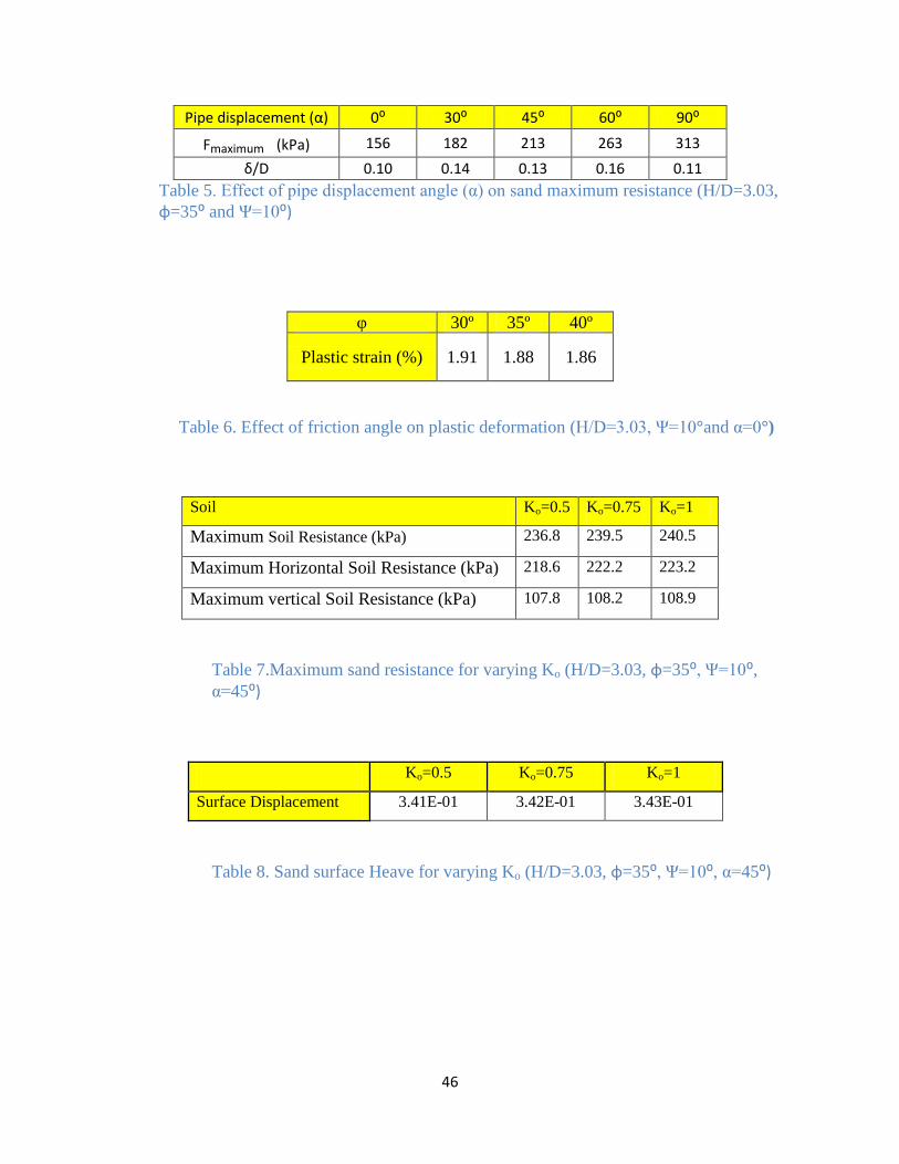
46
Pipe displacement (α) 0⁰ 30⁰ 45⁰ 60⁰ 90⁰
Fmaximum (kPa) 156 182 213 263 313
δ/D 0.10 0.14 0.13 0.16 0.11
Table 5. Effect of pipe displacement angle (α) on sand maximum resistance (H/D=3.03,
φ=35⁰ and Ψ=10⁰)
φ 30º 35º 40º
Plastic strain (%) 1.91 1.88 1.86
Table 6. Effect of friction angle on plastic deformation (H/D=3.03, Ψ=10°and α=0°)
Soil Ko=0.5 Ko=0.75 Ko=1
Maximum Soil Resistance (kPa) 236.8 239.5 240.5
Maximum Horizontal Soil Resistance (kPa) 218.6 222.2 223.2
Maximum vertical Soil Resistance (kPa) 107.8 108.2 108.9
Table 7.Maximum sand resistance for varying Ko (H/D=3.03, φ=35⁰, Ψ=10⁰, α=45⁰)
Ko=0.5 Ko=0.75 Ko=1
Surface Displacement 3.41E-01 3.42E-01 3.43E-01
Table 8. Sand surface Heave for varying Ko (H/D=3.03, φ=35⁰, Ψ=10⁰, α=45⁰)
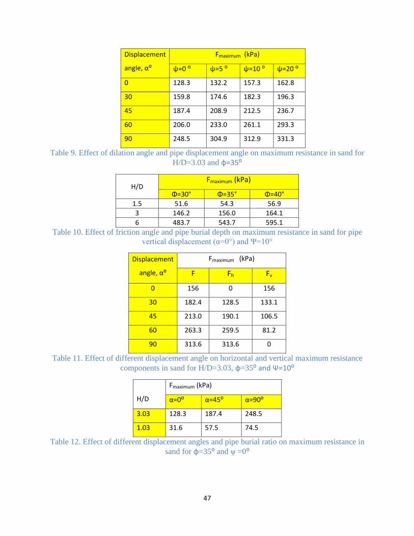
47
Displacement
angle, α⁰
Fmaximum (kPa)
ψ=0 ⁰ ψ=5 ⁰ ψ=10 ⁰ ψ=20 ⁰
0 128.3 132.2 157.3 162.8
30 159.8 174.6 182.3 196.3
45 187.4 208.9 212.5 236.7
60 206.0 233.0 261.1 293.3
90 248.5 304.9 312.9 331.3
Table 9. Effect of dilation angle and pipe displacement angle on maximum resistance in sand for
H/D=3.03 and φ=35⁰
H/D Fmaximum (kPa)
Φ=30° Φ=35° Φ=40°
1.5 51.6 54.3 56.9
3 146.2 156.0 164.1
6 483.7 543.7 595.1
Table 10. Effect of friction angle and pipe burial depth on maximum resistance in sand for pipe
vertical displacement (α=0°) and Ψ=10°
Displacement
angle, α⁰
Fmaximum (kPa)
F Fh Fv
0 156 0 156
30 182.4 128.5 133.1
45 213.0 190.1 106.5
60 263.3 259.5 81.2
90 313.6 313.6 0
Table 11. Effect of different displacement angle on horizontal and vertical maximum resistance
components in sand for H/D=3.03, φ=35⁰ and Ψ=10⁰
H/D
Fmaximum (kPa)
α=0⁰ α=45⁰ α=90⁰
3.03 128.3 187.4 248.5
1.03 31.6 57.5 74.5
Table 12. Effect of different displacement angles and pipe burial ratio on maximum resistance in
sand for φ=35⁰ and ψ =0⁰

48
Table 13. Effect of pipe-soil friction coefficient on maximum resistance in sand for H/D=3.03,
φ=35⁰ and ψ=10⁰
φ ⁰ ψ ⁰ H/D Nqv
(ALA)
Fv/ϒHD
(FEM)
Qu (kPa)
(ALA)
Fv (kPa)
(FEM)
⁰ ⁰ kPa kPa
30 10 3 2. 2.8 131.5 146.2
35 10 3 2.4 3.0 149.4 156.0
40 10 3 2.7 3.1 167.3 164.1
35 0 3 2.4 2.8 149.4 146.6
35 5 3 2.4 2.9 149.4 150.7
35 10 3 2.4 3.0 149.4 156.0
35 20 3 2.4 3.1 149.4 162.9
35 30 3 2.4 3.2 149.4 170.2
35 10 1.5 2.4 2.0 61.9 54.2
35 10 3 2.4 2.9 149.4 155.8
35 10 4.5 2.4 3.6 221.9 289.6
35 10 6 2.4
5.1 295.9 543.7
Table 14.Comparision between bearing capacity factors and soil maximum
resistances estimated from ALA (2001) and finite element modeling in sand
α⁰
Fmaximum (kPa)
Friction
Coeff.=0.25
Friction
Coeff.=0.44
Friction
Coeff.=1
0 155.8 155.8 155.8
45 212.5 212.5 212.5
90 312.6 312.7 312.6
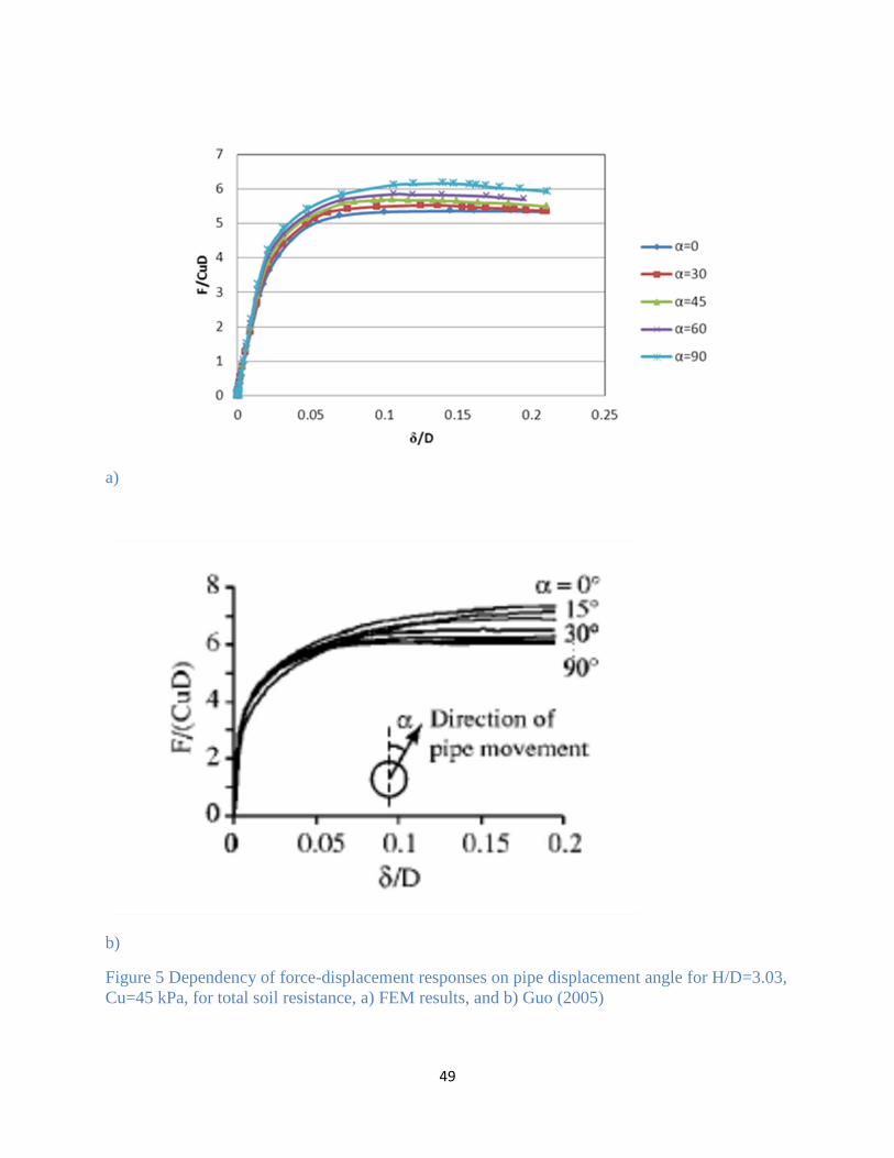
49
a)
b)
Figure 5 Dependency of force-displacement responses on pipe displacement angle for H/D=3.03,
Cu=45 kPa, for total soil resistance, a) FEM results, and b) Guo (2005)

50
a)
b)
Figure 6 Dependency of force-displacement responses on pipe displacement angle for
H/D=3.03, Cu=45 kPa, for the horizontal component of soil resistance a) FEM results,
and b) Guo (2005)
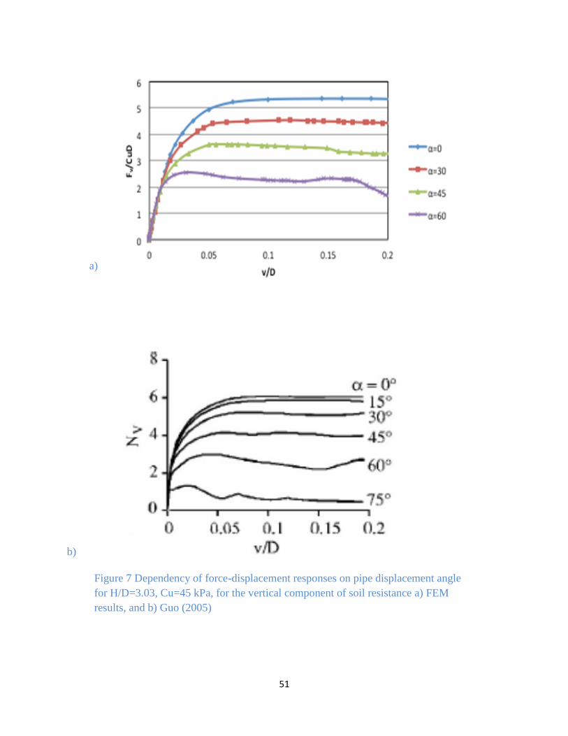
51
a)
b)
Figure 7 Dependency of force-displacement responses on pipe displacement angle
for H/D=3.03, Cu=45 kPa, for the vertical component of soil resistance a) FEM
results, and b) Guo (2005)

52
Figure 8. Deformed finite element mesh as a result of pipe vertical displacement of
δ/D=0.3, α=0⁰, (Cu=45 kPa, H/D=3.03), Displacement contours (m)
Figure 9. Deformed finite element mesh as a result of pipe oblique displacement of
δ/D=0.3, α=45⁰, (Cu=45 kPa, H/D=3.03), Displacement contours (m)
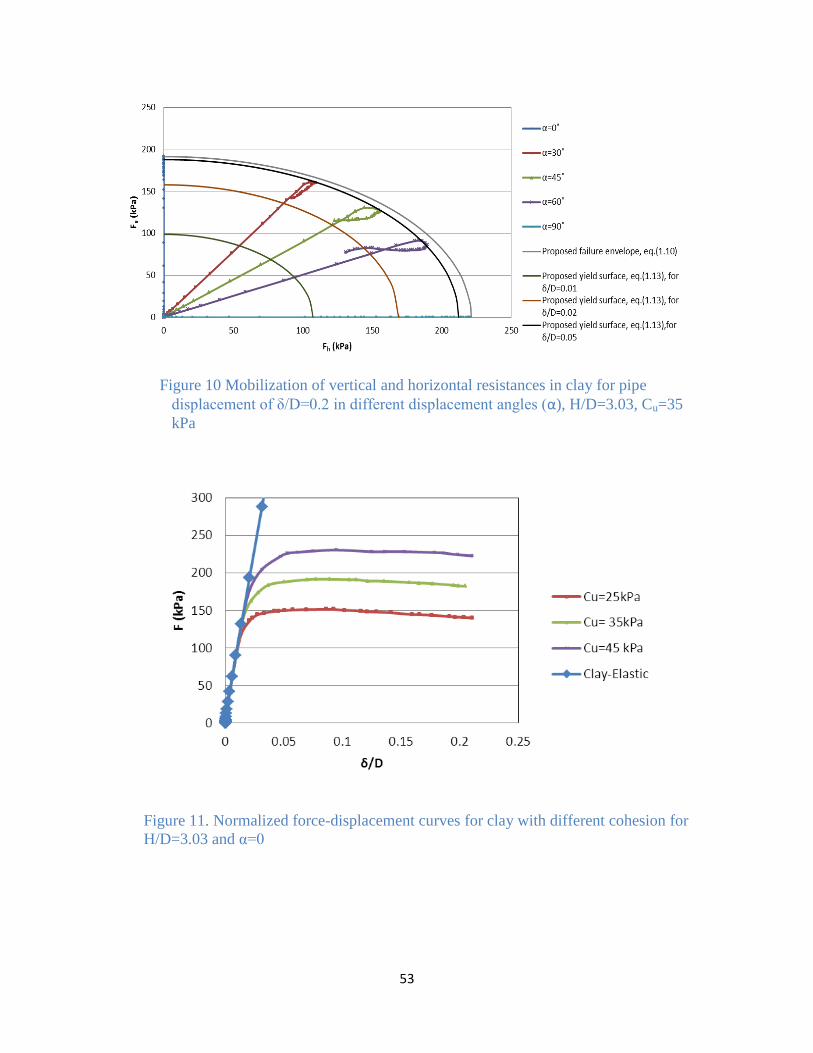
53
Figure 11. Normalized force-displacement curves for clay with different cohesion for
H/D=3.03 and α=0
Figure 10 Mobilization of vertical and horizontal resistances in clay for pipe
displacement of δ/D=0.2 in different displacement angles (α), H/D=3.03, Cu=35
kPa
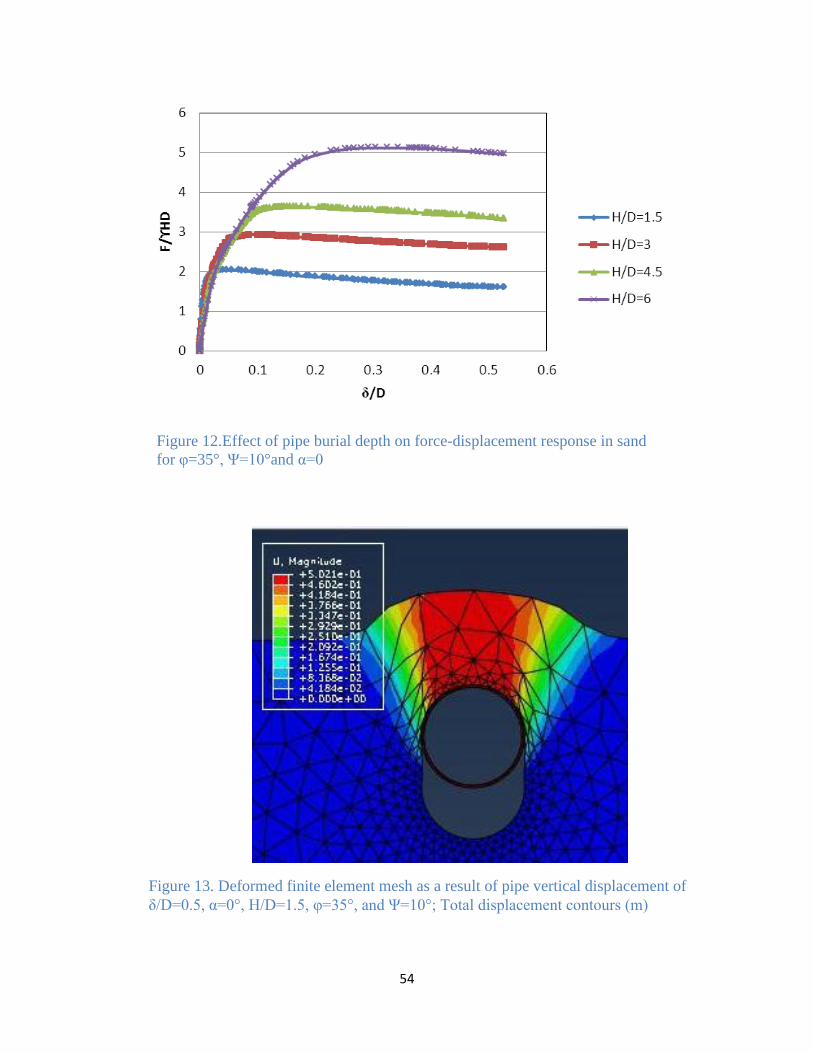
54
Figure 12.Effect of pipe burial depth on force-displacement response in sand
for φ=35°, Ψ=10°and α=0
Figure 13. Deformed finite element mesh as a result of pipe vertical displacement of
δ/D=0.5, α=0°, H/D=1.5, φ=35°, and Ψ=10°; Total displacement contours (m)

55
Figure 14. Deformed finite element mesh as a result of pipe vertical displacement
of δ/D=0.5, α=0°, H/D=6, φ=35°and Ψ=10°; Displacement contours (m)
Figure 15. Deformed finite element mesh showing the plastic zone developed in
sand as a result of pipe vertical displacement of δ/D=0.5, H/D= 1.5, φ=35°and
Ψ=10°. Plastic strain contours (%).
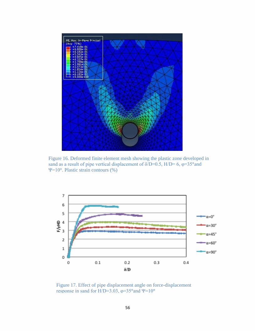
56
Figure 16. Deformed finite element mesh showing the plastic zone developed in
sand as a result of pipe vertical displacement of δ/D=0.5, H/D= 6, φ=35°and
Ψ=10°. Plastic strain contours (%)
Figure 17. Effect of pipe displacement angle on force-displacement
response in sand for H/D=3.03, φ=35°and Ψ=10°
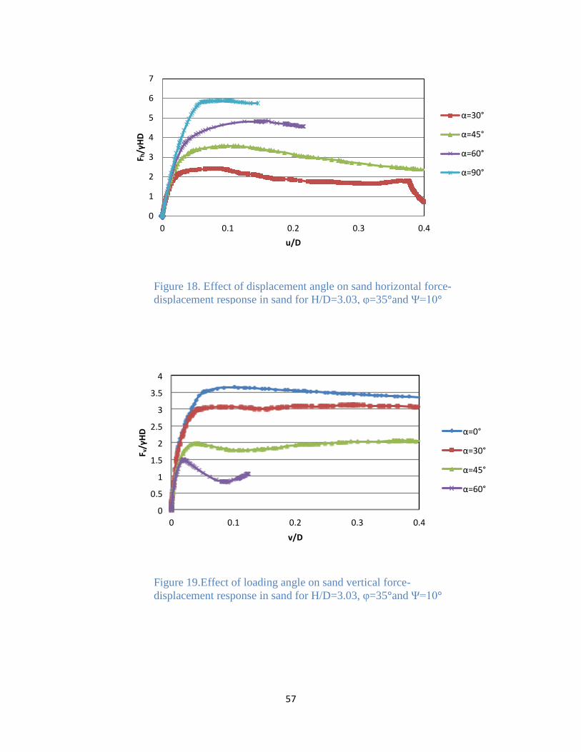
57
0
1
2
3
4
5
6
7
0 0.1 0.2 0.3 0.4
F h/γ
HD
u/D
α=30°
α=45°
α=60°
α=90°
0
0.5
1
1.5
2
2.5
3
3.5
4
0 0.1 0.2 0.3 0.4
F v/γHD
v/D
α=0°
α=30°
α=45°
α=60°
Figure 18. Effect of displacement angle on sand horizontal force-
displacement response in sand for H/D=3.03, φ=35°and Ψ=10°
Figure 19.Effect of loading angle on sand vertical force-
displacement response in sand for H/D=3.03, φ=35°and Ψ=10°
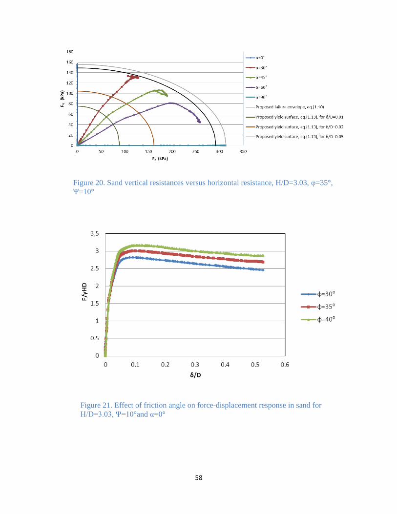
58
Figure 21. Effect of friction angle on force-displacement response in sand for
H/D=3.03, Ψ=10°and α=0°
Figure 20. Sand vertical resistances versus horizontal resistance, H/D=3.03, φ=35°,
Ψ=10°
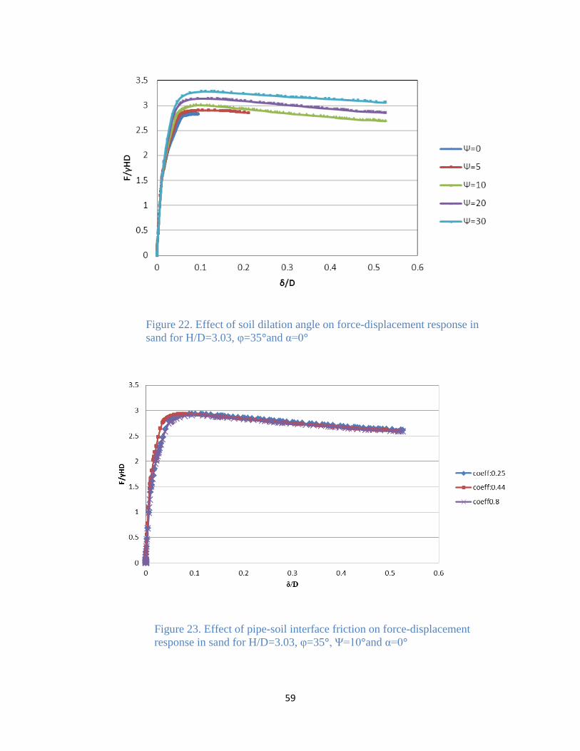
59
Figure 22. Effect of soil dilation angle on force-displacement response in
sand for H/D=3.03, φ=35°and α=0°
Figure 23. Effect of pipe-soil interface friction on force-displacement
response in sand for H/D=3.03, φ=35°, Ψ=10°and α=0°
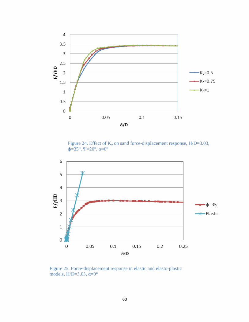
60
Figure 24. Effect of Ko on sand force-displacement response, H/D=3.03,
φ=35⁰, Ψ=20⁰, α=0⁰
Figure 25. Force-displacement response in elastic and elasto-plastic
models, H/D=3.03, α=0°
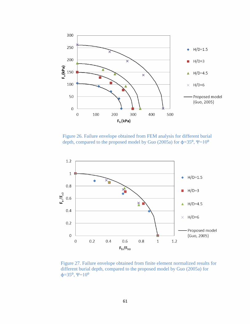
61
Figure 26. Failure envelope obtained from FEM analysis for different burial
depth, compared to the proposed model by Guo (2005a) for φ=35⁰, Ψ=10⁰
Figure 27. Failure envelope obtained from finite element normalized results for
different burial depth, compared to the proposed model by Guo (2005a) for
φ=35⁰, Ψ=10⁰
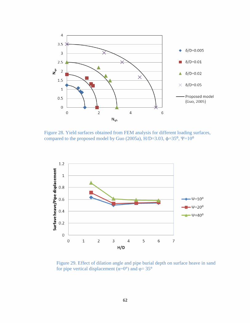
62
Figure 28. Yield surfaces obtained from FEM analysis for different loading surfaces,
compared to the proposed model by Guo (2005a), H/D=3.03, φ=35⁰, Ψ=10⁰
Figure 29. Effect of dilation angle and pipe burial depth on surface heave in sand
for pipe vertical displacement (α=0°) and φ= 35°
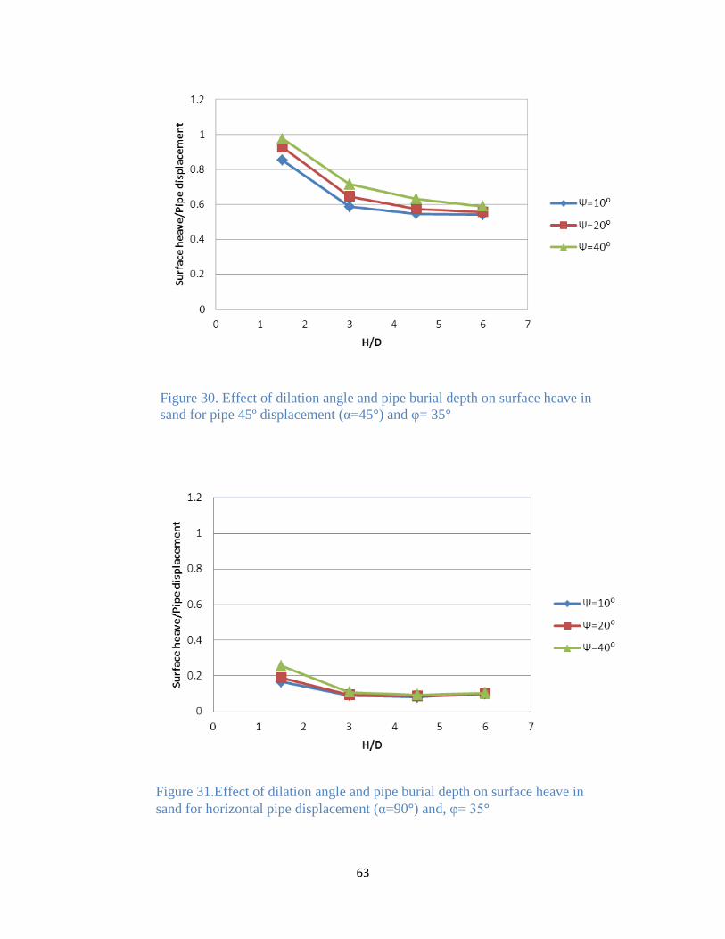
63
Figure 31.Effect of dilation angle and pipe burial depth on surface heave in
sand for horizontal pipe displacement (α=90°) and, φ= 35°
Figure 30. Effect of dilation angle and pipe burial depth on surface heave in
sand for pipe 45º displacement (α=45°) and φ= 35°
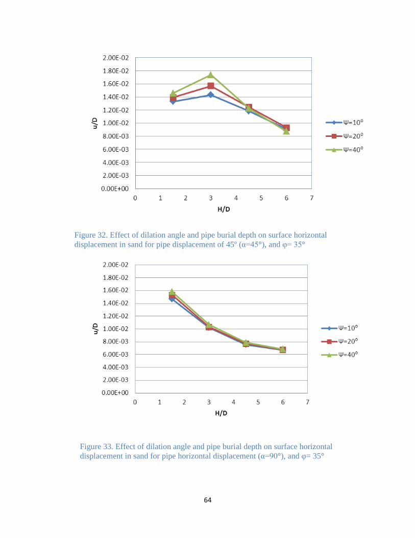
64
Figure 33. Effect of dilation angle and pipe burial depth on surface horizontal
displacement in sand for pipe horizontal displacement (α=90°), and φ= 35°
Figure 32. Effect of dilation angle and pipe burial depth on surface horizontal
displacement in sand for pipe displacement of 45º (α=45°), and φ= 35°
65
Chapter four: Conclusion
4.1 Conclusion
In this project, the effect of soil parameters on the soil maximum resistance has been
studied using finite element modeling, while the pipe is subjected to varying
displacement angles.
The proposed failure envelope (Guo, 2005a) has been compared to the results from the
finite element model. The comparison indicates agreement between the finite element
model and the proposed failure envelope for both cohesive and frictional soils.
Also, the maximum soil resistances calculated from the finite element modeling have
been compared to those predicted from ALA guideline. In general the results are in the
same range obtained from the finite element analysis. In most conditions the results
estimated from ALA (2001) are more conservative comparing to those calculated from
the finite element modeling, except for the shallow pipes (H/D<2), zero dilation angle
and high friction angles where the finite element modeling provides more conservative
results. Since the dilation angle, pipe-soil interaction and in-situ stress have not been
considered in ALA equations, for using the guideline a safety factor is needed. Based
on the results from finite element modeling, a safety factor needs to be applied to the
results predicted by ALA to have accurate and conservative results in pipe-soil design.
At the end, the effects of soil parameters such as dilatancy, friction angle, in-situ stress
coefficient, the pipe-soil friction coefficient, and the pipe burial depth ratio on the soil
maximum resistance have been investigated. The results show that the maximum
normal force per unit length depends on the type of soil surrounding the pipe. By

66
comparing all the results pipe burial depth, soil cohesion, friction and dilation angles
were found to have a significant effect on pipe-soil interaction and can considerably
increase the maximum soil resistance.
The effects of the in-situ stress coefficient and pipe-soil friction coefficient on the soil
maximum resistance are of less importance. By changing the pipe-soil friction
coefficient, the maximum soil resistance changes less than 1%, which indicates the
negligible effect of pipe roughness on the soil maximum resistance with any pipe
displacement angle. Also by increasing the in-situ stress coefficient of soil from 0.5 to
1, the maximum soil resistance increases 1.5% which can be negligible.
In addition, results indicate that the larger pipe displacement angle (α) will result in a
higher soil maximum resistance and as a result a pipe-soil interaction subjected to a
horizontal pipe displacement (α=90°) exhibit higher collapse loads.
The FEM results also indicate that by increasing the pipe burial depth, the surface
heave and pipe horizontal displacement become independent of soil dilation angle.
4.2 Recommendation for further studies
There are several more parameters affecting pipe-soil interaction which was not
considered in this project, such as soil porosity, water content, and soil creep behavior.
It is recommended to consider the effect of pore water pressure on pipe-soil interaction
in future studies.
Also, further studies are required to validate the model using data from experiments on
pipe-soil interactions under pipe oblique displacement.
67
References
Achmus, A., Abdel-Rahman, Kh. (2005). Numerical modeling of vertical piles in clay under inclined
compression loading. Frontiers in Offshore Geotechnics (pp. 391-396). Perth, Australia: Taylor &
Francis.
Allotey, N., & El Naggar, M. (2008). Generalized dynamic Winkler model for nonlinear soil-structure
interaction analysis. Canadian Geotechnical Journal, 45(4), 560-573.
Al-Mhaidib, A. (2005). Shearing rate effect on interfacial friction between sand and steel. The fifteenth
International Offshore and Polar Engineering Conference. 2, pp. 633-640. Seoul, Korea: The
Internation Society of Offshore and Polar Engineers (ISOPE).
Audibert, J.M.E, Nyman, K.J. (1977). Soil restraint against horizontal motion of pipes. ASCE Journal of
Geotechnical Engineering Division, 103(10), 1119-1142.
Badv, K., Daryani, K.E. (2010). An investigation into the upward and lateral soil-pipeline interaction in
sand using finite difference method. Iranian Journal of Science amd Technology,Transaction B:
Engineering, 34(4), 433-445.
Cai, G., Liu, S., Puppal, A., Tong, L. (2011). Assessment of the coefficient of lateral earth pressure at rest
(Ko) from in situ seismic tests. ASTM Geotechnical Testing Journal, 34(4), 310-320.
Canadian Geotechnical Society. (1992). Canadian Foundation Engineering Manual. Vancouver: The
Canadian Geotechnical Society.
Carrier, W. (2005). Pipeline supported on a nonuniform Winkler soil model. Geotechncial and
Geoenvironmental Engineering, 131(10), 1301-1304.
Daiyan, N., Kenny, S., Phillips, R., Popescu, R. (2011). Investigating pipeline-soil interaction under axial-
lateral relative movements in sand. Canadian Geotechncial Journal, 48(11), 1683-1695.
Daiyan, N., Kenny, S., Phillips, R., Popsecu, R. (2010). Investigation of axial/lateral interacion of pipes in
dense sand. Physical modeling in Geotechnics. 1, pp. 619-624. Zurich, Switzerland: CRC Press.
Das, B. (1985). Resistance of shallow inclined anchors in clay. Uplift behavior of anchor foundations in
soil. ASCE. 1, pp. 86-101. New York: S. M. Clemence, ed.
Debasis, D. (2006). Fintie element method: concepts and applications in geomechanics. New Dehli:
Prentice-Hall of India Private Limited.
Guo, P. (2005a). Numerical modeling of pipe-soil interaction under oblique loading. Journal of
Geotechnical and Geoenvironmental Engineering, 131(2), 260-268.
Guo, P., Stolle, D. (2005b). Lateral pipe-soil inetraction in sand with reference to scale effect. Journal of
Geotechnical and Geoenvironmental Engineering, 131(3), 338-349.
68
Hobbs, B.E, Ord, A., Marone, C. (1990). Dynamic behavior of rock joints. International Society of Rock
Mechanics. 1, pp. 435-445. Leon, Norway: A.A.Balkema.
Leonards, G. (1965). Experimental study of static and dynamic friction between soil and typical
construction materials. New Mexico: Air force weapons laboratory.
Liu, R., Li,B., Wang, H., Zhang, J., Xu, Y. (2011). Studies of soil resistance for buried pipeline uplift in sand.
Rock and Soil Mechanics, 32(1), 27-32.
Merifield, R., White, D.J, Randolph, M.F. (2008). The ultimate undrained resistance of the partially
embedded pipelines. Geotechnique, 58(6), 461-470.
Merifield, R.S, White, D.J, Randolph, M.F. (2009). The effect of pipe-soil interface conditions on the
undrained breakout resistance of partially-embedded pipelines. Journal of Geotechnical and
Geoenvironmental Engineering, 136(6), 819-829.
Meyerhof, G. G., Hanna, A. M. (1978). Ultimate bearing capacity of foundation on layered soil under
inclined load. Canadian Geotechnical Journal, 15(4), 565–572.
National Energy Board. (2009). Focus on safety and environment, a comparative analysis of pipeline
performance. Canada: The Publication Office, National Energy Board.
Nyman, K. (1984). Soil response against the oblique motion of pipes. ASCE Journal of Transportation
Engineering, 110(2), 190-202.
Pipeline&Hazardous Materials Safety Administration. (2013). Significant pipeline incidents. Retrieved
from U.S. Department of Transportation:
http://primis.phmsa.dot.gov/comm/reports/safety/SigPSI.html?nocache=4790#_all
Rizkalla, M., Trigg, A., Simmonds, G. (1996). Recent advances in the modeling of longitudinal
pipeline/soil interaction for cohesive soils. 15th International Conference on Offshore Mechanics
and Arctic Engineering. 1, pp. 325-332. ASME.
Rowe, R.K, Davis, H. (1982). The behavior of anchor plate in sand. Geotechnique, 32(1), 25-41.
Taylor, D. (1948). Fundamentals of Soil mechanics. New York: Wiley.
Trautmann, C.H, O'Rourke, T.D. (1985). Lateral force‐displacement response of buried pipe. Geotech
Engineering, 111(9), 1077-1092.
Winkler, E. (1867). Die lehre von elastizitat und festigkeit (Teaching on elasticity and stiffness). Prague,
Czechoslovakia.
Yu, H.-S. (2006). Plasticity and geotechncis. Springer Science.
Zhand, X., Han, A., Wu, Z. (2011). Research on pipe-soil displacement transefr coefficient for buried
pipeline. Advanced Materials Research, 201, 201-203.
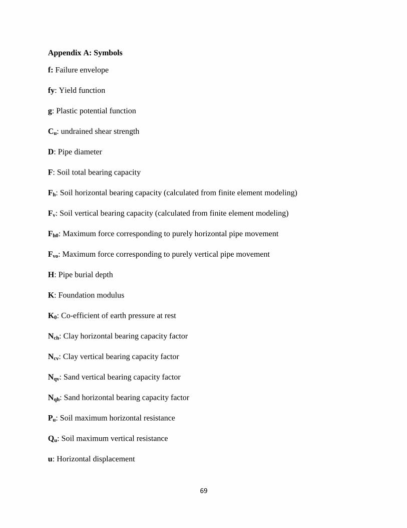
69
Appendix A: Symbols
f: Failure envelope
fy: Yield function
g: Plastic potential function
Cu: undrained shear strength
D: Pipe diameter
F: Soil total bearing capacity
Fh: Soil horizontal bearing capacity (calculated from finite element modeling)
Fv: Soil vertical bearing capacity (calculated from finite element modeling)
Fh0: Maximum force corresponding to purely horizontal pipe movement
Fvo: Maximum force corresponding to purely vertical pipe movement
H: Pipe burial depth
K: Foundation modulus
K0: Co-efficient of earth pressure at rest
Nch: Clay horizontal bearing capacity factor
Ncv: Clay vertical bearing capacity factor
Nqv: Sand vertical bearing capacity factor
Nqh: Sand horizontal bearing capacity factor
Pu: Soil maximum horizontal resistance
Qu: Soil maximum vertical resistance
u: Horizontal displacement
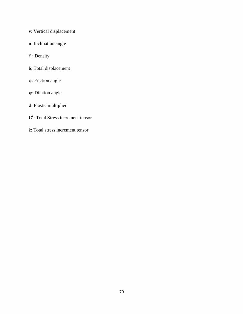
70
v: Vertical displacement
α: Inclination angle
ϒ : Density
δ: Total displacement
φ: Friction angle
ψ: Dilation angle
: Plastic multiplier
Ce: Total Stress increment tensor
: Total stress increment tensor
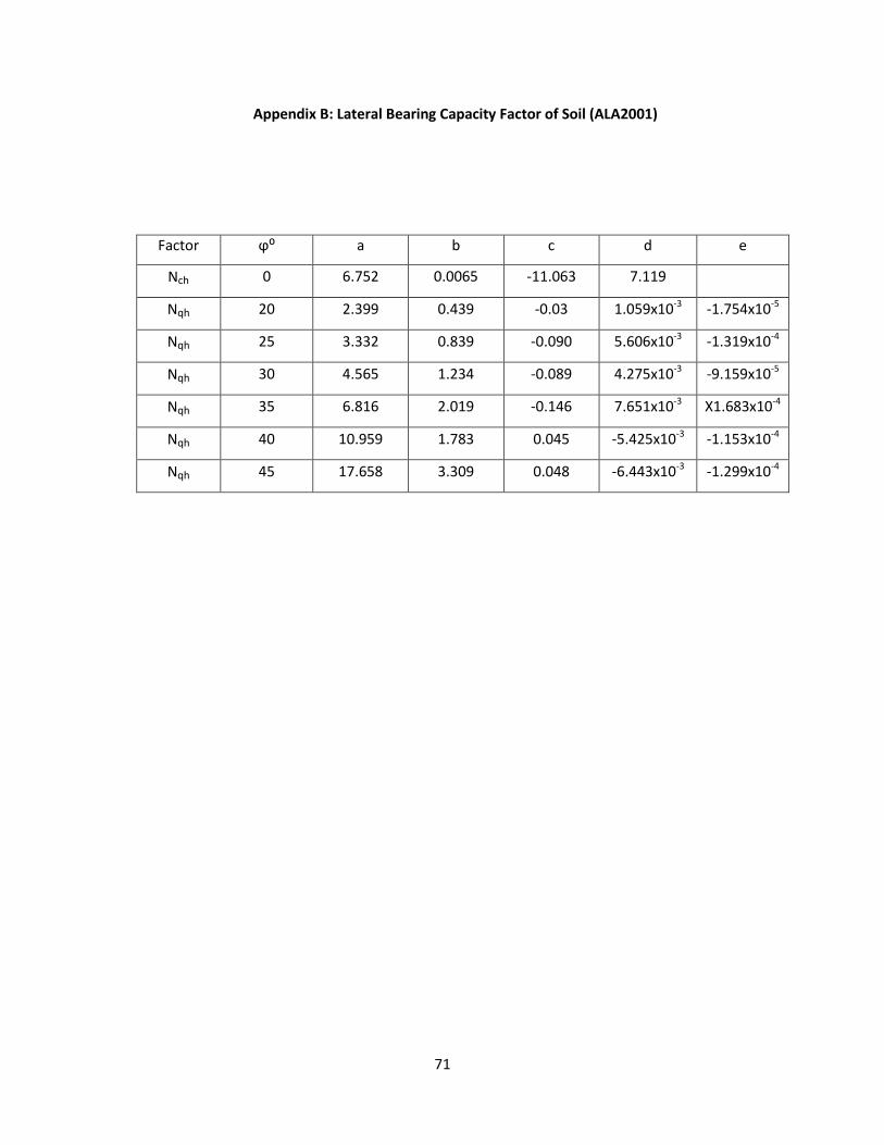
71
Appendix B: Lateral Bearing Capacity Factor of Soil (ALA2001)
Factor ϕ⁰ a b c d e
Nch 0 6.752 0.0065 -11.063 7.119
Nqh 20 2.399 0.439 -0.03 1.059x10⁻³ -1.754x10⁻⁵
Nqh 25 3.332 0.839 -0.090 5.606x10⁻³ -1.319x10⁻⁴
Nqh 30 4.565 1.234 -0.089 4.275x10⁻³ -9.159x10⁻⁵
Nqh 35 6.816 2.019 -0.146 7.651x10-3 X1.683x10-4
Nqh 40 10.959 1.783 0.045 -5.425x10⁻³ -1.153x10⁻⁴
Nqh 45 17.658 3.309 0.048 -6.443x10⁻³ -1.299x10⁻⁴


