
1
U.S. recession forecasting using probit models with asset index
predictor variables
Thomas Hsu
Economics Department
The University of Maryland Baltimore County
Professor Chunming Yuan, Advisor
Professor David Mitch, Graduate Director
Professor Thomas Gindling, Graduate Director
November, 2016

2
Abstract
A considerable amount of research exists using probit models to predict a binary
recession indicator variable. The single predictor variable which has demonstrated the greatest
predictive potential to date is the yield spread, the difference between the yields on long-term
and short-term Treasury securities. The most recent two recessions (2001 and 2008) were
preceded by historic asset bubbles, the first due to inflated stock prices and the second due
primarily to inflated home prices. Two metrics of asset bubbles in combination were found to be
remarkably good indicators of these latest recessions with an out-of-sample predictive power
exceeding that of the yield spread. The Cyclically Adjusted Price Earnings Ratio (CAPE) was
found to give both a better in-sample fit and better predictive power than then S&P 500.

3
“All models are wrong. Some are useful.”
Attributed to George Box
“The only function of economic forecasting is to make astrology look respecta-
ble.”
Attributed to John Kenneth Galbraith
“I don’t even know what a bubble means. These words have become popular. I
don’t think they have any meaning.”
Eugene Fama (2010)
“In the garden, growth has it seasons. First comes spring and summer, but then
we have fall and winter. And then we get spring and summer again.”
Chance, the gardener, Being There (film, 1979)

1
Introduction
Predicting Business cycles presents the greatest forecasting problem in macroeconomics
in term of both its importance and its challenge. Recessionary periods can bring considerable
hardship to many, especially the unemployed and their dependents. Advanced notice of
impending recession is of interest to households, firms and investors. Given that business cycle
stabilization policy is generally seen as a responsibility of government, accurate forecasts of
business cycle peaks and troughs are of particular interest to central bankers and policy makers.
Incorrectly timed counter cyclical policy actions may be ineffective or even aggravate
fluctuations.
The National Bureau of Economic Research (NBER) is commonly accepted as the
official arbiter of recession dates in the United States and started publishing business cycle dates
in 1929. Determining business cycle turning points is now the responsibility of the Business
Cycle Dating Committee of the NBER, started in 1978. The NBER developed a methodology for
the empirical analysis of business cycles using the definition suggested by Burns and Mitchell
(1946): “business cycles are co-movements of several macroeconomic variables which determine
the turning points, peaks and troughs, in aggregate economic activity.” Recessions start just
following a peak and end at a trough, representing the period of broadly declining economic
activity, and expansions follow a trough and end at a peak. These cycles are reoccurring but not
periodic. The NBER states that “[a] recession is a significant decline in economic activity spread
across the economy, lasting more than a few months, normally visible in production,
employment, real income, and other indicators.” It is “marked by widespread contraction in
many sectors of the economy …, normally visible in real GDP, real income, employment,
industrial production, and wholesale-retail sales.”

2
It is popular in the financial press to define a recession as beginning with two consecutive
quarters of decline in GDP. While the NBER considers GDP the single best measure of aggregate
economic activity, it considers the GDP definition to be too narrow a measure of economic
activity to reliably date recessions. So for example, the 2001 recession did not include two
consecutive quarters of negative growth. Nevertheless, declines in GDP are closely correlated to
recession periods (see graph). Since GDP estimates by the Bureau of Economic Analysis (BEA)
of the Department of Commerce are only available quarterly, the BCDC uses monthly estimates
of GDP by the private forecasting firm of Macroeconomic Advisers.
Figure 1
GDP growth and recessions for the period of this study, 1955Q1 to 2016Q2. Note that not
all recessions begin with two quarters of negative growth.
-15
-10
-5
0
5
10
15
20
0
1
55 60 65 70 75 80 85 90 95 00 05 10 15
Recession
GDP growth rate (percent)
BCDC uses a variety of monthly indicators with particular emphasis on personal income
less transfer payment (in real terms) and employment. Also there are two indicators with
coverage primarily of manufacturing and goods: industrial production and the volume of sales

3
and the manufacturing and wholesale-retails sectors (adjusted for price changes). The NBER
employs “no fixed rule about which other measures contribute information to the process.”
(NBER)
The BCDC approach is retrospective. They wait until sufficient data are available to
avoid major revisions. In determining the onsets of recessions they wait until they are confident
that “even in the event that activity begins to rise again immediately, it has declined enough to
meet the criterion of depth. As a result, we tend to wait to identify a peak until many months
after it actually occurs.”(NBER)
Typically, the BCDC declares the start of recessions after the fact anywhere from 6 to 18
months, “long enough so that the existence of a recession is not at all in doubt.” (NBER)
Likewise, for the troughs: 6 to 18 months. Peak and trough months are determined and the
BCDC takes no stand on the date within the month. (This lag in reporting is relevant in the real-
time application of dynamic probit models, not to be confused with autoregressive probit models,
both discussed later in this paper, where a lagged value of the recession indicator is used as a
predictor variable). NBER announced the December 2007 peak a year later. Over the past 30
years, NBER announcement have been made from 6 to 20 months after a corresponding peak or
trough.
Table 1
NBER recession dates for the sample period
Peak Trough
August 1957 April 1958
April 1960 February 1961
December 1969 November 1970
November 1973 March 1975
January 1980 July 1980
July 1981 November 1982
July 1990 March 1991
March 2001 November 2001
December 2007 June 2009

4
Earlier attempts at forecasting economic cycles examined continuous or interval
dependent variables such as GDP, consumption and employment (Stock and Watson, 2003).
Much recent research has focused on predicting recessions as discrete states rather that making
quantitative estimations of future economic activity. Predicting recessions with a binary
recession indicator dates back at least to the 1990’s. Stock and Watson (1991) focused on
recessions as discrete events and thus predicted whether the economy was in a recession state or
not rather than forecasting continuous or interval variables such as GDP growth. Estrella and
Hardouvelis (1991) used a static probit model (discussed later in this paper) and many studies in
recent decades have used a binary indicator models for forecasting recessions (Dueker, 1997;
Estraella and Mishkin, 1997; Chauvet and Potter, 2005; Wright, 2006; Kauppi and Saikkonen,
2008; Nyberg, 2010; Ng, 2011; Fossati, 2015). An advantage of a binary recession indicator
variable is that it isolates the start and duration of recessions. On the other hand, studies of
continuous or interval dependent variables such as economic growth, mix information on the
magnitudes with that of the timing of the onset and duration of the economic cycles in their
measures-of-fit. Estrella and Mishkin (1998) point out that “[t]he discrete dependent variable
also sidesteps the problem of spurious accuracy associated with quantitative point estimates of,
for example, future real gross domestic product (GDP) growth” and that models forecasting
continuous economic variables suffer more from endogeneity problems than those giving
probabilities. Hamilton (1989) presents an empirical analysis that suggests that the economy
evolves differently within distinct discrete states, some corresponding to recessionary and
expansion periods.
Many recession leading indicators have been considered by researchers over recent
decades. One in particular has been repeatedly validated as perhaps the best predictor variable,

5
the difference between the yield on short and long-term U.S. Treasury securities, called the yield
spread, yield curve or term spread (Estrella and Trubin 2006). “Yield curve” refers to the plot of
yields versus maturity time span, which typically slopes upward depicting lower yield on short-
term securities and increasing yields as the maturities increase. A flattening or inversion of the
slope signals the onset of a recession anywhere from two to six quarters ahead. I will not discuss
the mechanisms connecting the yield curve to recessions other than to say that they are spooky
and mysterious.
Figure 2
A recent and typical yield curve from July, 2016 and a partially inverted yield curve from
March, 2007, prior to the January 2008 recession.
The literature on information in the yield spread related to forecasting recessions goes at
least as far back as Kessel, 1956. Fama (1984) discusses the relationship between the term
structure and business cycles. Stock and Watson (1991) use a version of the yield spread as well
as a number of other leading indicators including housing permits, manufacturing orders, indices
of exchange rates, employment and financial variables other that the yield spread. They suggest
that important omitted variables such stock prices and consumer sentiment might improve the
models. Estrella and Hardouvelis (1991) discuss the power of the yield curve as a predictor of

6
economic activity, and specifically that the yield curve flattened and then inverted in 1989 in
advance of the 1990 recession. In addition to the term spread, Estrella and Mishkin (1997)
consider interest rates spreads, stock prices, monetary aggregates, macro indicators, and leading
indices of the Commerce Department and use a novel measure of predictive power, Estrella’s
pseudo R2, which is used in subsequent literature (Kauppi, 2008; Nyberg, 2010; Fossati, 2012;
Ng, 2012). As with much of the literature, they note that the 1990 recession seemed uniquely
difficult to forecast. They find that overfitting is a serious problem in macroeconomic prediction
and that the in-sample and out-of-sample performance can differ greatly. The yield curve again
shines as a forecasting variable. Dueker (1997) uses a dynamic probit model in which a lag of the
depended indicator is used as a predictor variable in the model, a “probit analogue of adding a
lagged dependent variable to a linear regression model” and used a probit model with Markov
switching as well. His predictors included the Commerce Department’s index of leading
indicators, M2 money growth, and change in Standard and Poor’s 500 index of stock prices.
Moneta (2003) shows the effectiveness of yield spreads in the Euro Zone and that the yield curve
outperforms the OECD Composite Leading Indicator for the Euro Area, the quarterly growth rate
of the stock price index, and GDP growth especially beyond one quarter. Chauvet and Potter
(2005) use a model that takes into account the predictive instability of the yield curve, using
breakpoints across business cycles.
Wright (2006) finds the federal funds rate in addition to the term spread improves the
predictive power of the probit models (but ruins out-of-sample result in my experience). Wright
uses the RMSE to measure out-of-sample fit. Kauppi and Saikkonen (2008) used dynamic
models and iterated forecasting and again relied on the interest rate spread “as the driving
predictor.” Katayama (2010) uses a combination of 33 macroeconomic indicators with a 6-month

7
horizon including a combination of the term spread, change in the S&P 500 index and the growth
rate of non-farm employment. Katayama compares several cumulative probability distribution
functions in place of the cumulative normal function of the probit model, preferring the Laplace
CDF. Nyberg (2011) includes domestic and foreign yields spread and stock market returns in a
dynamic probit model. He also uses a dynamic autoregressive model using a lagged value of the
latent variable and the recession indicator dependent variable as predictors as well as an
interactive term of the lagged dependent variable and the spread variable. His out-of-sample
period includes the 2001 and 2008 recessions. He examines German recessions as well as U.S.
recession and confirm the domestic term spread as an important predictor.
Eric Ng (2011) incorporates various recession risk factors, including financial market
expectations, credit or liquidity risks, asset price variables (as in this paper) and macroeconomic
fundamentals in addition to the term spread in advanced dynamic probit models. He finds that
while dynamic models outperformed static models, and dynamic autoregression models were
only marginally better still. Static models did as good a job at forecasting the onset of recessions.
Serena Ng and Wright (2013) focus on the Great Recession which they say is unlike most
postwar recession in “being driven by deleveraging and financial market factors” and how it
differs from those driven by supply and monetary policy shocks. To this they attribute the failure
of economic models and predictors, such as the term spread, that work well otherwise, to predict
this most recent recession. Fossati (2015) also found that “models that use only financial
indicators exhibit a large deterioration in fit after 2005.” He obtains substantial improvements
over Estrella and Mishkin (1998), Wright (2006) and Katayama (2010). He finds as well that
models using macro factors are more robust to revisions in indicator values ex post compared to
vintage data.

8
Data
Both of the two most recent recessions were preceded by unsustainable asset bubbles
much greater than any others in the sample period 1955 to 2016 (see Figure 5 and Figure 7).
Some previous literature (Ng, 2011; Fossati,2012; Christiansen et al, 2013) considered asset
effects as precedents of recessions in their models. Part of the contribution of this paper is to test
whether pre-2000 recession data can be used to estimate a model forecasting this century’s
recessions. The special character of the 2001 and 2008 recessions puts into question whether
information from prior history can be used to forecast these two recent recessions. This objective
motivates my choice of variables to include an equity index and a home price index, and of my
choice of the in-sample period to include approximately the last four and a half decades of the
20th century, and an out-of-sample to start from 2000q1. Ng (2011) uses an inflation adjusted
S&P equity index and a Case-Shiller Home Price Index. But to the best of my knowledge, these
two effects were not considered in isolation or jointly in comparison to the yield spread or in
combination with the yield spread alone as I do in this study. Furthermore, the equity price
indices used in previous literature (Ng, 2011; Fossati,2012; Christiansen et al, 2013) are not a
measures of the general price level as compared to historical earnings and so do not necessarily
reflect market overvaluation as does the Cyclically Adjusted Price Earnings ratio (also known as
the Shiller PE Ratio), which I use here. I chose only the yield spread and two asset measures as
predictors so as to determine the relative effectiveness of the information in the term spreads as
compared to that in the asset indices and to specifically focus on these variables alone in the
general interests of parsimony. Our principle interest is the out-of-sample performance. In-
sample fit can always be improved by adding more variables but this does not necessarily lead to
better out-of-sample performance, and in fact, frequently makes it worse. A contribution of this

9
paper is to compare the predictive power of the asset variables to the benchmark yield spread.
As mentioned, for equity assets, the specific variable I chose is the Cyclically Adjusted
Price Earnings ratio (CAPE). It is the ratio of the S&P index level to the ten-year inflation
adjusted earnings of the index. Since the intrinsic value is the present value of the long-run
returns, the CAPE can thus be seen as an indicator of an overpriced market or “bubble”. The
CAPE reflects deviations of equity prices from their fundamental values. A change in the CAPE
would reflect market a deviation away from, or return toward and theoretical steady state of
“correct” valuation and it is the changes in the CAPE that in theory would be reflected in
changes in the state of the overall macroeconomy. Hence, I use the first difference of the CAPE
in the model. A plausible mechanism of action of the CAPE on the recession state is that the
wealth effect of inflated equity prices creates high aggregate demand which abruptly sinks when
the market quickly corrects. The reduced aggregate demand is accompanied by general economic
doldrums which constitute the recession. The CAPE may as well be a reflection of economic
conditions antecedent to recession. The actual CAPE variable used in the calculations in this
study is normalized by dividing by the average over the sample period.
Instead of the CAPE, other authors (Ng, 2011; Fossati,2012; Christiansen et al, 2013) use
market indices such as the S&P 500 or PE ratio. However, the CAPE’s use of a longer run
earnings average smooths the volatility of short-term earnings and medium term general
economic cycles and hence better reflects the market’s long-term earnings in comparison to
current prices. The CAPE is a better metric of overvaluation of stocks since it is a ratio of
contemporary price to long-term historical returns. A comparison of the two variables as to their
effectiveness in the model is made below in the section on model selection. Figure 3 CAPEd1
and change in S&P 500., below, compares the percent change in the S&P 500 to the first

10
difference of the CAPE variable, hereafter designated CAPEd1. The two variables generally
track each other closely, as would be expected, but at times one may deviate more severely than
the other. Note in particular, that the swings of the CAPE in 2000, prior to the 2001 recession,
are more extreme than those of the changes in the S&P 500.
Figure 3 CAPEd1 and change in S&P 500.
-.3
-.2
-.1
.0
.1
.2
.3
55 60 65 70 75 80 85 90 95 00 05 10 15
CAPE d1 SP500 percent change/100
The variable I chose as metric of housing bubble is the Case-Shiller Home Price Index
(CS). It is available with a two-month lag and is frequently subject to revision. The sizes of the
revisions are of little consequence to this study and my results are robust to these ex-post
alterations in the CS. Many other economic indicators are determined and announced with
considerable delay and are often revised after the fact as well. For example, GDP figures are
available about three months after the end of a quarter, and as mentioned, announcements of the
beginning of recessions are, at best, available 6 months after the fact. Both the CAPE and the
variable reflecting the term spread are available in real time, are precise, and generally are not

11
subject to ex-post revisions as is typical of macroeconomic indicators. The variable CS used in
this study is normalize by dividing by the average value over the sample period.
Robert Shiller (2013) found that “[h]ome prices look remarkably stable when corrected
for inflation. Over the 100 years ending in 1990 — before the recent housing boom — real home
prices rose only 0.2 percent a year, on average” yet house prices rose by about 90% between
1996 and 2007 (Shiller 2007). By contrast real rent increased by only about 5% in the same peri-
od. Hence the “dramatic price increase [of house prices] is hard to explain, since economic fun-
damentals do not match up with the price increases.” (Shiller, 2007) On the basis of this, one
might say that the CS reflects home price deviations from some theoretical intrinsic values since
it compares general market prices to their historic prices. It compares current prices to a sort of
long-term average using repeat sale prices and so reflects whether the market is in a normal or
abnormal price state. Like the equity market, the market for houses is not efficient but subject to
animal spirits sometimes resulting in irrational exuberance. As in the case of the CAPE, a high
CS produces a wealth effect and a sudden drop in the CS can foretell an economic slowdown.
My dynamic model uses the quarter t-2 recession state, which is not known in real-time.
However, for forecasting the start of a recession on an ongoing basis, one might assume that the
current and last quarters are non-recession ones. It is generally recognized that the economy is in
a recession a quarter or two into one. Nonetheless, the dynamic model here assumes
unrealistically, that the current recession state and previous ones are known. If the dynamic
model does not show a distinct advantage over the static models, even given this unrealistically
perfect information up to date, then under realistic circumstances it could only fare worse.
I use quarterly data of recession states and follow Kauppi and Saikkonen (2006) in
defining a quarter as the first quarter of a recession if its first month or the proceeding quarter’s

12
second or third moth is classified as the NBER business cycle peak and classify a given quarter
as the last quarter of a recession period if its second or third month or the subsequent quarter’s
first month is classified as the NBER business cycle trough. For reasons mentioned, the in-
sample period is from 1955q1 to 1999q4.
For a term spread variable, market analysts often use the difference between the ten-year
and two-year Treasury rates. Some academic researchers have used the spread between the ten-
year Treasury and federal funds rate. Most common in the literature using probit models to
predict recessions is the spread between the 10-year bond yield and the 3-month Treasury bill
rate which I adopted here, in part to be able to make comparison between our findings here and
those in the literature. I will call this variable spread. Advantages and disadvantages of different
rates are discussed in Estrella and Trubin (2006). The data for the Treasury securities are readily
available at the Federal Reserve Economic Data website or the U.S. Treasury Department
website.
A glance at the graphs of each of the three variables I use shows information each
contains with respect to recessions. In the graph for spread, note small or negative spread prior to
all the recessions in the sample.
Figure 4
The yield spread
-2
-1
0
1
2
3
4
0
1
55 60 65 70 75 80 85 90 95 00 05 10 15
Recession
Yield spread (10 year less 3 month yield)

13
A graph of CAPE and recessions over the data set is given below. Note distinct peak prior
to 2001 recession as well as smaller peaks before the 1970, 1973, and 2008 recessions.
Figure 5
Cyclically
Adjusted Price
Earnings Ratio
(CAPE)
Figure 6
First-differences
of the Cyclically
Adjusted Price
Earnings Ratio
5
10
15
20
25
30
35
40
45
0
1
55 60 65 70 75 80 85 90 95 00 05 10 15
Recession
Cyclically adjusted price-to-earnings ratio
-.3
-.2
-.1
.0
.1
.2
.3
0
1
55 60 65 70 75 80 85 90 95 00 05 10 15
recession CAPE first differences
14
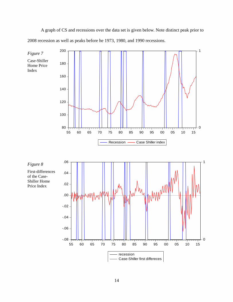
A graph of CS and recessions over the data set is given below. Note distinct peak prior to
2008 recession as well as peaks before he 1973, 1980, and 1990 recessions.
Figure 7
Case-Shiller
Home Price
Index
Figure 8
First-differences
of the Case-
Shiller Home
Price Index
80
100
120
140
160
180
200
0
1
55 60 65 70 75 80 85 90 95 00 05 10 15
Recession Case Shiller index
-.08
-.06
-.04
-.02
.00
.02
.04
.06
0
1
55 60 65 70 75 80 85 90 95 00 05 10 15
recession
Case-Shiller first differeces

15
Econometric model
In consideration of models, let ty be the binary indicator variable which equals one at
time t if and only if the economy in a recession state at time t. We wish to forecast the time
series 1{ }T
t ty
where
1, the economy is in a NBER determined recession at time
0, the economy is not in a recession at time t
ty
t
.
We will let r be the recession recognition lag, the number of time periods that pass before
the recession state of the economy is known, and s be the data availability lag for the explanatory
variable x.
Conditional on the information set
1 - - -1{ , ,..., , ,...}t h t j t j t k t ky y x x where j h r k h s , available at time t h , ty has a
Bernoulli distribution
( )t t h ty B p
where ( 1)t t h tp P y , the conditional probability. Because ty takes values 0 or 1, its expected
value is ( )t h t tE y p . If -t kx is the vector of explanatory variables in the static probit model, a
linear function of the exogenous explanatory variables gives the value of an unobserved variable
t t kx
from which the probability is determined from the cumulative normal distribution function
2 21( 1) ( )
2
t u
t h t tP y e du
.
Katayama (2010) considered other cumulative distribution functions in place of and found

16
that some right-skewed distributions increased the proportion correctly predicted. Lowing the
threshold of a “correct” prediction from 50% can have a similar effect.
The parameters of the model are estimated by the criteria of a maximum likelihood
function
1
1
( , ) ( ) [1 ( )]t t
Ty y
t t t
t
L y
,
or equivalently a maximum log likelihood function
1
( , ) { log ( ) (1 ) log[1 ( )]}T
t t t t t
t
y y y
L .
Because the static model neglects the serial dependence of the recession variable it may
produce misleading or implausible recession probability forecasts. If the previous state of the
economy is not included in the model, it does not take into account the autocorrelative structure
of the binary time series. The solution proposed by Dueker (1997) is to remove the serial
correlation by using a lag of the recession indicator, thus using information in the autocorrelative
structure of the dependent variable, a probit analogue of adding a lagged dependent variable to a
linear regression model. This so-called dynamic probit model uses past values of the recession
variable as a predictor variable on the right-hand-side of the equation for the latent variable
function.
t t k t lx y
for a single lag of y and
q
t t k l t l
l h r
x y
for multiple lags. In application, it is only feasible to include t jy for j h r , where r is the
number of periods of the delay in recognition of a recession state.

17
Kauppi and Saikkonen (2008) consider the autoregressive probit model where the latent
variable is given as
1t t k tx
having a lag of itself as a predictor. Combined with the dynamic model this gives the dynamic
autoregressive specification
1t t k t l tx y .
Ng (2011) finds that the dynamic autoregressive specification adds little to the fit and predictive
power of the dynamic model alone. We will not consider autoregressive models further in this
study.
The effects of predictors may take many periods to be felt and may not work their way
through the economy for many periods still. A change in independent variable tx may affect
multiple subsequent values of the outcome ty ,1ty ,… This can be accounted for in an infinite
distributed lag probit model
0
t k t k
k
x
wherein all previous lags of the predictor variable are included in the specification, or a finite
distributed lag model
0
q
t k t k
k
x
.
The general form for the latent variable specification in the dynamic finite distributed lag model
is thus
11 2
1, 1, 2, 2, , ,
0 0 0 0
...n nq qq q
t k t h k k t h k n k n t h k k t h k
k k k k
x x x y
.
The coefficients of the various lags give both the dynamic marginal effects and the cumulative

18
effects of the explanatory variable on the outcomes over time as well as how patterns in the lags
effect subsequent values of the outcome variable.
Once a model specification is decided and the parameters estimated, the fit and
explanatory power of the model is measured in a variety of ways. The McFadden Pseudo R2
(hereafter simply pseudo R2) corresponds to the coefficient of determination in standard linear
regression and likewise reflects the degree to which a model explains the variation in the
response variable.
2 logpseudo R 1
log
u
r
L
L ,
where uL is the likelihood function for the unrestricted model and rL that for the restricted
model.
For model comparison and model selection, the Akaike Information Criterion (AIC) and
the Schwarz, or Bayesian, Information Criterion (BIC) are used, where smaller values reflect
more efficient models in the sense of providing greater explanatory power but not at the expense
of parsimony of explanatory variables.
BIC 2
log 2logk T LT
,
AIC 2
logk LT
,
where k is the number of parameters to be estimated, T the number of in-sample observations,
and L is the likelihood as a function of the estimated parameters. Note that the effect of k in the
expressions penalizes for additional parameters.
For measures of out-of-sample fit, I use the root-mean-square-error (RMSE), mean-
absolute-error (MAE), and Theil inequality coefficient as well as the percent of correct

19
predictions, of true positives, of false positives, of true negatives and of false negatives.
RMSE 2
1
1( )
T
t t
t T
p yr
,
MAE 1
1 T
t t
t T
p yr
,
and
Theil inequality coefficient =
2
1
2
1
( )T
t t
t T
T
t
t T
p y
y
,
where r is the number of out-of-sample periods.
Results
For the forecast horizon I chose a lags of two quarters, since that would be a minimum
amount of time for corrective monetary or fiscal policy to start taking effect. Static models with
single variables and their various lags were considered first. For a two quarter ahead forecast for
variables spread and CAPEd1 I started with lag -2 alone and successively added lags -3, -4 and
so forth while using the AIC, BIC and the significance of the last lag coefficient to decide how
many lags of each variable to use. Likewise, for CSd1, but starting at lag -3 since there is a two-
month delay in the release of the Case-Shiller index. The increase in the pseudo R2 as lags are
added was also considered in selecting the number of lags. If the increase in the R2 is not very
large compared to previous increases, this suggests that little explanatory power is added by the
additional lag. Finally, the joint significance of a variable and its lags in the model combining the
variables is considered as well to check for the overall significance of a variable and its lags.
For the variable spread, lags -2 to -5 were chosen on the basis of the lowest AIC and BIC
and the longest sequence of lags with the last lag’s coefficient being significant and for the fact
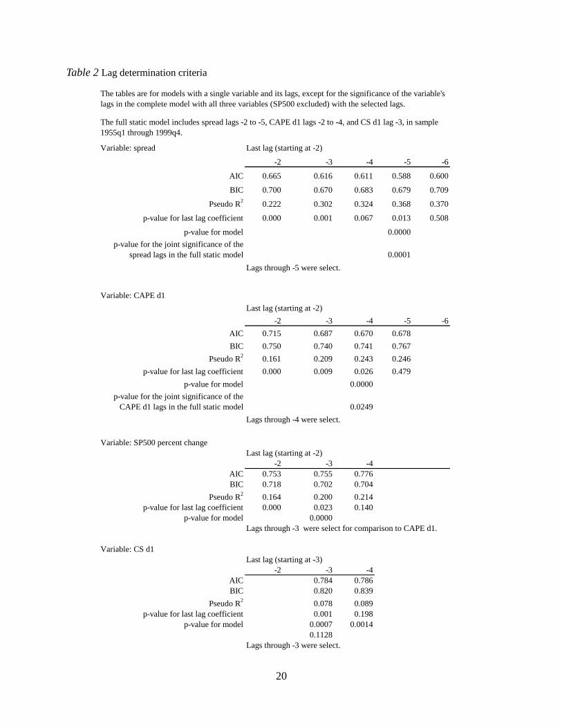
20
Table 2 Lag determination criteria
Variable: spread Last lag (starting at -2)
-2 -3 -4 -5 -6
AIC 0.665 0.616 0.611 0.588 0.600
BIC 0.700 0.670 0.683 0.679 0.709
Pseudo R2
0.222 0.302 0.324 0.368 0.370
p-value for last lag coefficient 0.000 0.001 0.067 0.013 0.508
p-value for model 0.0000
p-value for the joint significance of the
spread lags in the full static model 0.0001
Lags through -5 were select.
Variable: CAPE d1
Last lag (starting at -2)
-2 -3 -4 -5 -6
AIC 0.715 0.687 0.670 0.678
BIC 0.750 0.740 0.741 0.767
Pseudo R2
0.161 0.209 0.243 0.246
p-value for last lag coefficient 0.000 0.009 0.026 0.479
p-value for model 0.0000
p-value for the joint significance of the
CAPE d1 lags in the full static model 0.0249
Lags through -4 were select.
Variable: SP500 percent change
Last lag (starting at -2)
-2 -3 -4
AIC 0.753 0.755 0.776
BIC 0.718 0.702 0.704
Pseudo R2
0.164 0.200 0.214
p-value for last lag coefficient 0.000 0.023 0.140
p-value for model 0.0000
Lags through -3 were select for comparison to CAPE d1.
Variable: CS d1
Last lag (starting at -3)
-2 -3 -4
AIC 0.784 0.786
BIC 0.820 0.839
Pseudo R2
0.078 0.089
p-value for last lag coefficient 0.001 0.198
p-value for model 0.0007 0.0014
0.1128
Lags through -3 were select.
The full static model includes spread lags -2 to -5, CAPE d1 lags -2 to -4, and CS d1 lag -3, in sample
1955q1 through 1999q4.
The tables are for models with a single variable and its lags, except for the significance of the variable's
lags in the complete model with all three variables (SP500 excluded) with the selected lags.

21
that adding another lag barely increases the pseudo R2. For the variable CAPEd1, lags -2 to -4
were chosen on the basis of the lowest AIC, the very nearly the lowest BIC (no lag combination
has both lowest AIC and BIC) and longest lag sequence with the last lag’s coefficient being
significant. Also, an additional lag adds almost nothing to the Pseudo R2. Similar criteria were
used to select lag -3 alone for the CSd1 variable (see table 1). The percent change in the S&P 500
was similarly considered to compare its performance to the CAPE.
Figure 9, below, gives the probability of a recession state based on models with the CAPE
first difference and the percent change in the S&P 500 and their lags as the sole predictor
variables. A visual comparison of the predictive power of the S&P 500 variable and the CAPEd1
shows that the CAPEd1 produces a dramatically stronger and better timed forecast of the 2001
recession. Even for the in-sample, the pseudo R2 and the information criteria show the CAPEd1
and its optimal lags produce a better model than the S&P 500 percent change and its best lags.
Hence the CAPE has advantages that lead me to use it rather than the S&P 500 index as in for
example Ng 2011. Note that a strong, well timed signal of the onset of a recession is more useful
planners and central bankers than signal of the conclusion of a recession since the effect of
stimulatory policy extending beyond the conclusion of a recession seldom is as much cause for
much concern as a delay initiating stimulatory policy in advance of the onset of a recession.

22
Figure 9
Recession probabilities
based on the CAPE and
based on the S&P 500
Graphs of the probabilities of recession based solely on single variables and their lags
show that each contains valuable information on the timing of recession and furthermore
suggests that each variable contains information the others do not. The graph for the probability
computed using only spread (Figure 10) shows the information in the spread alone has predictive
power in signaling the beginnings of both the 2001 and 2008 recessions though the signals are
rather weak. The graph using the CAPEd1 variable alone (Figure 11) is remarkable for its
pronounced signals for both of the out-of-sample recessions but especially for the 2001 recession.
This is what one might expect given that that recession was associated with a stock bubble. It
predicts the onset of the 2001 recession precisely and with a very strong signal while its timing
on the 2008 recession is late. The CSd1 based graph (Figure 12) is remarkable as well. While it
fails to signal the 2001 recession it gives both a well-timed and very strong signal of the 2008
recession. Again, this is as we might expect for reasons analogous to those for the 2001 recession
being forecasted by stocks prices, the 2008 recession was signaled by home prices. The CAPE
0.0
0.2
0.4
0.6
0.8
1.0
55 60 65 70 75 80 85 90 95 00 05 10 15
Recession
CAPE d1 lags -2 to -4
SP500 percent change lags -2 to -3

23
and CS variables give complementary information. Each of the immediately following graphs
are for the estimated model given bellow the graph.
Figure 10
Recession probabilities based
on the spread
2 2 2 1 3 2 4 3 5 4( 1) ( ) ( )t t t t t t t tP y E y spread spread spread spread
Note the weaker signal of the two recent recessions but fewer false positive spikes than the model based on
asset variables alone.
Figure 11
Recession probabilities
based on the CAPE
2 2 2 1 3 2 4 3( 1) ( ) ( 1 1 1 )t t t t t t tP y E y CAPEd CAPEd CAPEd
Note the strong and timely signal for the 2001 recession. The 2008 is forecasted as well but late.
0.0
0.2
0.4
0.6
0.8
1.0
55 60 65 70 75 80 85 90 95 00 05 10 15
Recession
Probability based spread lags -2 to -5
0.0
0.2
0.4
0.6
0.8
1.0
55 60 65 70 75 80 85 90 95 00 05 10 15
Recession
Probability based CAPE 1st difference lags -2 to -4

24
Figure 12
Recession
probabilities based on
the CS
2 2 3 1( 1) ( ) ( 1 )t t t t tP y E y CSd
Note the failure to signal the 2001 recession but the strong signal and moderately good timing for the 2008
recession and several false positive peaks following.
Figure 13
Recession
probabilities based
on the CAPE and
the CS jointly
2 2 1 3 2 4 3 3 1( ) ( 1 1 1 1 )t t t t t tE y CAPEd CAPEd CAPEd CSd
The predictive power of the two asset variables together, static model (dynamic model, not shown, is very similar).
0.0
0.2
0.4
0.6
0.8
1.0
55 60 65 70 75 80 85 90 95 00 05 10 15
Recession
Probability based on CS first difference lag -3
0.0
0.2
0.4
0.6
0.8
1.0
55 60 65 70 75 80 85 90 95 00 05 10 15
recession
Probability based on CAPE d1 lags -2 to -4 and CS d1 lag -3.

25
The model with the combined asset variables and their lags
2 2 1 3 2 4 3 3 1( ) ( 1 1 1 1 )t t t t t tE y CAPEd CAPEd CAPEd CSd Equation 1
has a lager pseudo R2 than the one above for the spread lags alone and outperforms it on every
measure of out-of-sample fit except false positives/true negatives and the MAE. The response to
the asset variables for the out-of-sample recessions (Figure 13) is visually striking in the timing
and the strength of the signal, but does give considerably more false positives than the spread
variable and its lags give. More useful and actionable information is given by the asset variables
than the spread variable. and its lags. Table 2 below compares the performance measures of the
model with spread lags alone to that with only the asset variable lags alone.
Table 3
In sample factors
spread alone,
lags -2 to -5
CAPE d1 lags
-2 to -4 and
CS d1 lag -3
AIC 0.589 0.648
BIC 0.679 0.738
Pseudo R2
0.368 0.294
p-value for last lag
coefficient of the lags 0.013 0.027 and 0.005
Out of sample factors
RMSE 0.314 0.302
MAE 0.149 0.159
Theil Coef 0.584 0.378
false positive 1 6
false negative 9 1
true positve 0 8
true negative 56 51
Out-of-sample at 50% threshold.
9 recession and 57 non-recession quarters.
Distributed lags not only describe the persisting effect of changes in predictor variables,
but also capture information on how the relationship among the lags effects the dependent
variable. I use an unstructured distributed lag, not forcing any pre-specified relationship between

26
the lag coefficients. The collinearity of the lags, however, makes for very large standard errors
for the coefficient estimate and hence very large p-values for the individual lags. Our concern
however, is with the joint significance of the lags, the fit of the in-sample forecast, and most
importa
ntly, the predictive power in the out-of-sample forecast. As it turns out, the model fares
very well on all of these accounts. Information is captured by the model despite the uncertainty
of in estimates of the individual coefficients and that the predictive power of the model is stark
and impressive despite the very wide confidence intervals for the coefficient. The excellent fit of
the model both in and out-of-sample gives me confidence in the model as a whole. The
additional lags, however, add little to the predictive power and accuracy of the model out-of-
sample. Thus I adopt the following static and dynamic specifications which I will refer to as the
“full” or “complete” models.
2 2 1 3 2 4 3 5 4
2 1 3 2 4 3 3 1
( ) (
)
t t t t t t
t t t t
E y spread spread spread spread
CAPE CAPE CAPE CS
Equation 2
2 2 2 1 3 2 4 3 5 4
2 1 3 2 4 3 3 1
( ) (
)
t t t t t t t
t t t t
E y y spread spread spread spread
CAPE CAPE CAPE CS
Equation 3
Once the model with the combination of the variables and their lags was estimated, each
variable and its lags were tested for joint significance. Only the significance of the lag of CSd1
was poor with a p-value of 0.11 (Table 1 above). A comparison of the graphs of the restricted and
unrestricted model (Figure 15) for in-sample show very little difference. However, with the
benefit of foresight, estimating the model with an in-sample of 1955q1 through 2016q2 gives
similar coefficient (-38.6) but a p-value of 0.001 for CSd1 lag. Furthermore, it is our objective to
test the hypothesis that the 2008 recession would be forecast by a house price index. Thus for the

27
combined reasons, I chose to keep CSd1. As it turns out, the unrestricted model does much better
out-of-sample, especially so for the 2008 recession, again as we might expect.
Figure 14
Recession
probabilities based
on the spread, CS
and CAPE and
distributed lags
versus without
distributed lags
2 3 2 3( ) ( )t t t t tE y spread CAPE CS
2 2 1 3 2 4 3 5 4
2 1 3 2 4 3 3 1
( ) (
)
t t t t t t
t t t t
E y spread spread spread spread
CAPE CAPE CAPE CS
Distributed lags are found to add little to the predictive power of the model. The model without distributed
lags incorporates the best single lags.
0.0
0.2
0.4
0.6
0.8
1.0
55 60 65 70 75 80 85 90 95 00 05 10 15
recession
1st difs of CAPE and CS w/o dist lags
1st difs of CAPE and CS w/ dist lags

28
Figure 15
Recession probabilities
based on complete model
versus the complete model
less the CSd1 variable
2 2 1 3 2 4 3 5 4
2 1 3 2 4 3 3 1
( ) (
)
t t t t t t
t t t t
E y spread spread spread spread
CAPE CAPE CAPE CS
The CSd1 enhances the out-of-sample fit considerably, particularly with respect to strong, well-timed
forecasts of the onset of the 2008 recession.
Figure 16
Recession probabilities
based complete model
0.0
0.2
0.4
0.6
0.8
1.0
55 60 65 70 75 80 85 90 95 00 05 10 15
recession
Full static model less CSd1 variable
Full static model
0.0
0.2
0.4
0.6
0.8
1.0
55 60 65 70 75 80 85 90 95 00 05 10 15
Recession Full static model

29
2 2 1 3 2 4 3 5 4
2 1 3 2 4 3 2 1 3 2
( ) (
)
t t t t t t
t t t t t
E y spread spread spread spread
CAPE CAPE CAPE CS CS
Note the strong false positive in 1967 corresponding to a quarter with < 0.1% growth.
While it is not realistic to assume the forecaster will know the recession state of the
economy in real-time, for forecasting the onset of recession, one might assume that the current
quarter is in non-recession. Typically, after one or two quarters into a recession, it is apparent that
the general economy is in decline. We will assume for the dynamic model, unrealistically, that
we know the state of the economy in the quarter from which the forecast is made, that is, two
quarters in advance of the quarter to be forecasted. If even this model does not produce
substantial improvements of the static model, then it seems unlikely that a dynamic model, using
realistically obtainable data, would produce much of an improvement. More sophisticated
models, such as a dynamic autoregressive models and ones using iterated forecasting give
marginal improvements (cf. Kauppi and Saikkonen, 2008; Ng, 2011).
The dynamic model
2 2 2 1 3 2 4 3 5 4
2 1 3 2 4 3 3 1
( ) (
)
t t t t t t t
t t t t
E y y spread spread spread spread
CAPE CAPE CAPE CS
Equation 4
was estimated and compared to the static model. The static model does better on every criteria of
both in and out-of-sample fit, except of course, the pseudo R2.
What improvements to the model would we expect by adding lags of the outcome
variable? If a give quarter is not a recession quarter, the probability of the following quarter not
being a recession is quite high given that most quarters are not recessions quarters. If the current
quarter is a recession quarter, the following quarter is now much more likely to still be a
recession. Estimating the model 2 2( ) ( )t t tE y y , as seen from the graph below (Figure
18) of the probability, no practical predictive power is given by this simple dynamic model. If the

30
current quarter is a recession quarter, it gives the probability of two quarters ahead as being 0.46
and if the current quarter is not a recession then it gives the probability two quarters ahead as
being 0.09. Hence, we would not expect much of an improvement of the predictive power of the
dynamic over the static model. The lagged dependent variable may give us a better idea of the
duration of a recession but no useful information as to the onset of a recession. This is consistent
with the findings of Ng (2011).
Table 4 Comparison of the in-sample and out-of-sample performance of the models
In-sample 1955q1 through 1999q4
Factors
Static
model
Standard
errors*
Static
model
Standard
errors
Dynamic
model
Standard
errors*
constant -0.464 0.254 -0.609 0.205 -0.620 0.277
spread t-2 -0.211 0.248 -0.430 0.292
spread t-3 -0.527 0.363 -0.720 0.174 -0.470 0.370
spread t-4 0.232 0.364 0.242 0.381
spread t-5 -0.490 0.273 -0.328 0.299
CAPE d1 t-2 -8.912 3.710 -9.472 3.177 -7.447 3.850
CAPE d1 t-3 -0.480 3.807 0.376 3.899
CAPEd1 t-4 -5.550 3.996 -4.380 4.184
CS d1 -3 -34.043 21.702 -36.865 19.399 -29.761 21.676
y t-2 0.773 1.513
AIC 0.562 0.549 0.560
BIC 0.725 0.620 0.741
Pseudo R2
0.453 0.397 0.469
% correct in-sample
Out of sample 2000q1 to 2016q2
RMSE 0.156 0.150 0.173
MAE 0.074 0.075 0.083
Theil Ineq Coef 0.224 0.229 0.260
false positive 1 1 1
false negative 0 1 1
true positve 9 8 8
true negative 56 56 56
% correct 98.4 97.0 97.0
*See discussion on large standard errors
Out-of-sample at 50% threshold.
9 recession and 57 non-recession quarters.
Without distributed lags

31
Figure 17
Probabilities based
on the complete
static and complete
dynamic models
Figure 18
The simple
dynamic model
gives no practical
predictive power
as to the onset of
recessions.
2 2( ) ( )t t tE y y
Table 4 below gives the forecasted recession probabilities in the quarters leading up to the
two out-of-sample recessions. Recession quarters highlighted. The tables in the third column
0.0
0.2
0.4
0.6
0.8
1.0
55 60 65 70 75 80 85 90 95 00 05 10 15
Recession
Full static model
Full dynamic model
0.0
0.2
0.4
0.6
0.8
1.0
55 60 65 70 75 80 85 90 95 00 05 10 15
recession Dynamic model

32
give the estimated probabilities with the S&P 500 variable substituted for the CAPE variable.
The tables in the last column show the forecasted probabilities with the model parameters re-
estimated each successive quarter based on actual data from preceding quarters as so using all
available data at the time of the prediction.
Table 4 Forecasted recession probabilities.
Quarter Probability Actual Quarter Probability Actual Quarter Probability Actual Quarter Probability Actual
2000Q2 0.0037 0 2000Q2 0.0040 0 2000Q2 0.0229 0 2000Q2 0.0040 0
2000Q3 0.0246 0 2000Q3 0.0275 0 2000Q3 0.0269 0 2000Q3 0.0278 0
2000Q4 0.0664 0 2000Q4 0.0614 0 2000Q4 0.0473 0 2000Q4 0.0618 0
2001Q1 0.0662 0 2001Q1 0.0480 0 2001Q1 0.0531 0 2001Q1 0.0471 0
2001Q2 0.6801 1 2001Q2 0.7329 1 2001Q2 0.3226 1 2001Q2 0.7253 1
2001Q3 0.5969 1 2001Q3 0.7886 1 2001Q3 0.5343 1 2001Q3 0.7778 1
2001Q4 0.7735 1 2001Q4 0.8455 1 2001Q4 0.3366 1 2001Q4 0.8697 1
2002Q1 0.5834 0 2002Q1 0.6579 0 2002Q1 0.1912 0 2002Q1 0.7370 0
2002Q2 0.0459 0 2002Q2 0.0497 0 2002Q2 0.0226 0 2002Q2 0.0800 0
2002Q3 0.0004 0 2002Q3 0.0027 0 2002Q3 0.0003 0 2002Q3 0.0012 0
2002Q4 0.0022 0 2002Q4 0.0105 0 2002Q4 0.0013 0 2002Q4 0.0062 0
Quarter Probability Actual Quarter Probability Actual Quarter Probability Actual Quarter Probability Actual
2007Q1 0.2051 0 2007Q1 0.2273 0 2007Q1 0.2708 0 2007Q1 0.2454 0
2007Q2 0.2205 0 2007Q2 0.2289 0 2007Q2 0.2662 0 2007Q2 0.2250 0
2007Q3 0.2840 0 2007Q3 0.2709 0 2007Q3 0.2047 0 2007Q3 0.2486 0
2007Q4 0.3521 0 2007Q4 0.4195 0 2007Q4 0.5568 0 2007Q4 0.4794 0
2008Q1 0.6557 1 2008Q1 0.8060 1 2008Q1 0.7323 1 2008Q1 0.8244 1
2008Q2 0.3254 1 2008Q2 0.5124 1 2008Q2 0.5319 1 2008Q2 0.4922 1
2008Q3 0.9683 1 2008Q3 0.9780 1 2008Q3 0.8903 1 2008Q3 0.7807 1
2008Q4 0.7057 1 2008Q4 0.7589 1 2008Q4 0.6430 1 2008Q4 0.8661 1
2009Q1 0.8810 1 2009Q1 0.9144 1 2009Q1 0.5050 1 2009Q1 0.9476 1
2009Q2 0.8303 1 2009Q2 0.8929 1 2009Q2 0.8582 1 2009Q2 0.9745 1
2009Q3 0.2456 0 2009Q3 0.2383 0 2009Q3 0.2652 0 2009Q3 0.3684 0
2009Q4 0.4481 0 2009Q4 0.4613 0 2009Q4 0.0351 0 2009Q4 0.6575 0
2010Q1 0.0000 0 2010Q1 0.0000 0 2010Q1 0.0000 0 2010Q1 0.0000 0
2010Q2 0.0000 0 2010Q2 0.0000 0 2010Q2 0.0000 0 2010Q2 0.0000 0
Static model ongoing reestimation
Static model ongoing reestimation
Dynamic model Static model
Dynamic model Static model
Static model (S&P500)
Static model (S&P500)
The following graphs allow us to visually evaluated the robustness of the model to the
change of in-sample periods, that last using the period 1990-2016 to retrodict recessions in the
period 1955-1989.
Figure 19
0.0
0.2
0.4
0.6
0.8
1.0
55 60 65 70 75 80 85 90 95 00 05 10 15
In sample 1955q1 to 1984q4
33
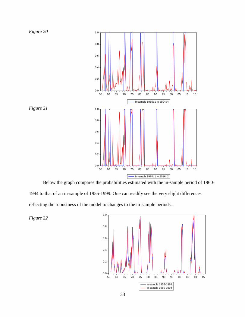
Figure 20
Figure 21
Below the graph compares the probabilities estimated with the in-sample period of 1960-
1994 to that of an in-sample of 1955-1999. One can readily see the very slight differences
reflecting the robustness of the model to changes to the in-sample periods.
Figure 22
0.0
0.2
0.4
0.6
0.8
1.0
55 60 65 70 75 80 85 90 95 00 05 10 15
In sample 1955q1 to 1994q4
0.0
0.2
0.4
0.6
0.8
1.0
55 60 65 70 75 80 85 90 95 00 05 10 15
In sample 1990q1 to 2016q2
0.0
0.2
0.4
0.6
0.8
1.0
55 60 65 70 75 80 85 90 95 00 05 10 15
In-sample 1955-1999
In-sample 1960-1994

34
Conclusion
To summarize, the major contributions and findings of this study are:
1) While the yield spread has for decades been recognized as the benchmark predictor of
recessions, the two asset variables together have predictive power, in terms of actionable
information, that exceeds that of the yield curve for the in and out-of-sample of this study.
2) This is so even though the in-sample is for a period wherein the recessions were not so
markedly characterized as being preceded by asset bubbles as the 2001 and 2008 recession were.
The in-sample period consisting of the last four and a half decades of the 20th century contains
information on the relationship between the two asset index variables and the recession indicator
that is captured by the estimated model and expressed in the two out-of-sample recessions. So
while the last two recessions may have had particularly pronounced antecedent causes in
historically large asset bubbles, the results here suggest they are not qualitatively different in this
regard from those of the previous four decades.
3) The CAPE produces both a better in-sample fit and substantially superior out-of-
sample forecasts than the standard indices as used in previous studies (cf. Ng, 2011; Fossati,
2012; Christiansen et al, 2013).
4) The complete model (Eq. 2) estimated here provides truly actionable information for
central bankers and policy makers concerned with counter-cyclical interventions.

35
References
Akerlof, George A. and Shiller, Robert J. Animal Spirits: How Human Psychology Drives the
Economy, and Why It Matters for Global Capitalism. Princeton University Press (2009).
Almon, Shirley. "The Distributed Lag Between Capital Appropriations and Expenditures."
Econometrics 33.1 (1965): 178. Web.
Beckers, Benjamin. "The Real-Time Predictive Content of Asset Price Bubbles for Macro
Forecasts." German Institute for Economic Research (2015): n. pag. Web.
Burns, A. F., and W. C. Mitchell. "Measuring Business Cycles." National Bureau of Economic
Research (n.d.): n. pag. Web.
Business Cycle Dating Committee. "The NBER's Recession Dating Procedure." National Bureau
of Economic Research (2008): n. pag. Web.
Cassidy, John. “Interview with Eugene Fama.” The New Yorker, January 13, 2010 .
Chauvet, Marcelle, and Simon Potter. "Forecasting Recessions Using the Yield Curve." SSRN
Electronic Journal SSRN Journal (2005): n. pag. Web.
Christiansen, Charlotte, Jonas Nygaard Eriksen, and Stig Vinther Møller. "Forecasting US
Recessions: The Role of Sentiments." SSRN Electronic Journal SSRN Journal (2013-14): n. pag.
Web.
Diebold, Francis X., and Glenn D. Rudebusch. "Scoring the Leading Indicators." The Journal of
Business J BUS 62.3 (1989): 369. Web.
Dueker, Michael J. "Strengthening the Case for the Yield Curve as a Predictor of United States
Recessions." Federal Reserve Bank of St.Louis Review 79 (1997): n. pag. Web.
Estrella, Arturo, and Gikas A. Hardouvelis. "The Term Structure as a Predictor of Real Economic
Activity." The Journal of Finance 46.2 (1991): 555. Web.
Estrella, Arturo. "A New Measure of Fit for Equations with Dichotomous Dependent Variables."
Journal of Business & Economic Statistics 16.2 (1998): 198. Web.
Estrella, Arturo, and Frederic S. Mishkin. "Predicting U.S. Recessions: Financial Variables as
Leading Indicators." Review of Economics and Statistics 80.1 (1998): 45-61. Web.
Estrella, Arturo, and Frederic S. Mishkin. "The Yield Curve as a Predictor of U.S. Recessions."
Current Issues in Economics and Finance (1996): n. pag. Web.
Estrella, A., and Mary R. Trubin. "The Yield Curve as a Leading Indicator: Some Practical
Issues." Current Issues in Economics and Finance 12.5 (2006): n. pag. Web.

36
Estrella, Arturo. "Why Does the Yield Curve Predict Output and Inflation?" The Economic
Journal 115.505 (2005): 722-44. Web.
Estrella, Arturo. "The Yield Curve as a Leading Indicator: Frequently Asked Questions." Federal
Reserve Bank of New York (2009): n. pag. Web.
Fama, Eugene F., 1984, “The information in the term structure” Journal for Financial Economics
13, 509-528.
Haubrich, Joseph G., Sara Millington, and Brendan Costello. “Comparing Price-to-Earnings Ra-
tios: The S&P 500 Forward P/E and the CAPE”. Economic Trends, Federal Reserve Bank of
Cleveland, August 10, 2014.
Jackman, Simon. “Time Series Models for Discrete Data: solutions to a problem with quantita-
tive studies of international conflict.” Working paper. July 21, 1998. Web.
Kessel, Reuben A., 1956, “The cyclical behavior of the term structure of interest rates”
Occasional paper 91, National Bureau of Economic Research, New York
Filardo, Andrew J. "How Reliable Are Recession Prediction Models?" Federal Reserve Bank of
Kansas City (1999): n. pag. Web.
Fossati, Sebastian. "Forecasting US Recessions with Macro Factors." Applied Economics 47.53
(2015): 5726-738. Web.
Gerlach, Stefan, and Henri Bernard. "Does the Term Structure Predict Recessions? The
International Evidence." SSRN Electronic Journal SSRN Journal (n.d.): n. pag. Web.
Greene, William H. Econometric Analysis. 7th ed. Boston, Mass.: Pearson, 2012. Print.
Haltmaier, Jane. "Predicting Cycles in Economic Activity." SSRN Electronic Journal SSRN
Journal (2008): n. pag. Web.
Hamilton, James D. “A New Approach to the Economic Analysis of Non-
stationary Time Series and the Business Cycle." Econometrica, 57(1989), 357-84.
Hamilton, James D. "Calling Recessions in Real Time." International Journal of Forecasting
27.4 (2011): 1006-026. Web.
Hao, Lili, and Eric C. Y. Ng. "Predicting Canadian Recessions Using Dynamic Probit Modelling
Approaches." Canadian Journal of Economics/Revue Canadienne D'économique 44.4 (2011):
1297-330. Web.
Jong, Robert M. De, and Tiemen Woutersen. "Dynamic Time Series Binary Choice."
Econometric Theory 27.04 (2011): 673-702. Web.

37
Katayama, M. "Improving Recession Probability Forecasts in the U.S. Economy (unpublished)."
Louisiana State University (2009): n. pag. Web.
Kauppi, H. "Yield-curve Based Probit Models for Forecasting U.S. Recessions: Stability and
Dynamics." Helsinki Center of Economic Research (2008): 221. Web.
Kauppi, Heikki, and Pentti Saikkonen. "Predicting U.S. Recessions with Dynamic Binary
Response Models." Review of Economics and Statistics 90.4 (2008): 777-91. Web.
Marcellino, Massimiliano. "Chapter 16 Leading Indicators." Handbook of Economic Forecasting
(2006): 879-960. Web.
Levanon, Gad. "Evaluating and Comparing Leading and Coincident Economic Indicators." Bus
Econ Business Economics 45.1 (2010): 16-27. Web.
Mariano, Roberto S., and Yasutomo Murasawa. "A New Coincident Index of Business Cycles
Based on Monthly and Quarterly Series." J. Appl. Econ. Journal of Applied Econometrics 18.4
(2003): 427-43. Web.
Moneta, Fabio. "Does the Yield Spread Predict Recessions in the Euro Area?*." European
Central Bank: Working Paper Series 294 (2003): 263-301. Web.
National Bureau of Economic Research. “The NBER's Business Cycle Dating Procedure:
Frequently Asked Questions.” http://www.nber.org/cycles/recessions_faq.html November 2,
2016
Ng, Serena, and Jonathan H. Wright. "Facts and Challenges from the Great Recession for
Forecasting and Macroeconomic Modeling." Journal of Economic Literature 51.4 (2013): 1120-
154. Web.
Nyberg, Henri. "Dynamic Probit Models and Financial Variables in Recession Forecasting."
Journal of Forecasting J. Forecast. 29.1-2 (2010): 215-30. Web.
Proano, C. R. "Recession Forecasting with Dynamic Probit Model under Real Time Conditions."
Macroeconomic Policy Institute (IMK) (2010): n. pag. Web.
Rudebusch, Glenn D., and John C. Williams. "Forecasting Recessions: The Puzzle of the
Enduring Power of the Yield Curve." Journal of Business & Economic Statistics 27.4 (2009):
492-503. Web.
Shiller, Robert J. “Understanding Recent Trends in House Prices and Home Ownership”,
National Bureau of Economic Research working paper. October 2007.
Shiller, Robert J. “Why Home Prices Change (or Don’t).” New York Times. April 13, 2013.

38
Silvia, John, Sam Bullard, and Huiwen Lai. "Forecasting U.S. Recessions with Probit Stepwise
Regression Models." Bus Econ Business Economics 43.1 (2008): 7-18. Web.
Stock, James H., and Mark W. Watson. "New Indexes of Coincident and Leading Economic
Indicators." NBER Macroeconomics Annual 4 (1989): 351-94. Web.
Stock, James H., and Mark W. Watson. "Predicting recessions." Manuscript, Northwestern
University, 1991.
Watson.Mark W. "Using econometric models to Predicting recessions." Economic Perspectives,
November/December 1991.
Wright, Jonathan H. "The Yield Curve and Predicting Recessions." Finance and Economics
Discussion Series 7 (2006): n. pag. Web.


