
VISUAL OTTHYMO
USER’S MANUAL
VERSION 5.0
Civica Infrastructure Inc. August 2017


iii
CONTENTS
1 INTRODUCTION 1
1.1 Welcome 1
1.2 What’s New in Version 5.0 1
1.3 About the User’s Manual 2
1.4 VO Help Support 2
1.4.1 Documentation 3
1.4.2 Program Help File 3
1.4.3 Help Search 3
1.4.4 Context-Sensitive Help (F1) 3
1.4.5 Seminars and Workshops 3
1.5 Customer Support 3
1.6 Software License Agreement 4
1.7 Installing Visual OTTHYMO 7
1.7.1 Hardware and Software Requirements 7
1.7.2 Licensing System 8
1.7.3 Installation VO 8
1.7.4 Running VO 11
1.7.5 Uninstall VO 12
2 QUICK START TUTORIAL 13
2.1 Example Study Area 13
2.2 Project Setup for Sigle-event Model 13
2.3 Creating Drainage Network on Canvas 14
2.4 Setting Hydrologic Object Properties 16
2.5 Adding Design Storm 17
2.6 Running Single-event Simulations 19
2.7 Viewing Single-event Simulation Outputs 20
2.8 Converting to Continuous OTTHYMO Model 22
iv
2.9 Adding Long-term Precipitation and Temperature 23
2.10 Running Continuous Simulations 23
2.11 Viewing Continuous Simulation Outputs 24
3 CONCEPTUAL MODEL 28
3.1 Introduction 28
3.2 Visual OTTHYMO Hydrologic Objects Overview 29
3.3 Common Parameters 31
3.4 Flow Generation Hydrologic Objects 32
3.4.1 StandHyd 32
3.4.2 NasHyd 34
3.4.3 WilHyd 35
3.4.4 ScsHyd 36
3.5 Flow Routing Hydrologic Objects 37
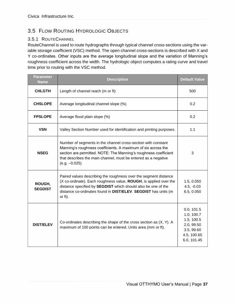
3.5.1 RouteChannel 37
3.5.2 MuskingumCunge 38
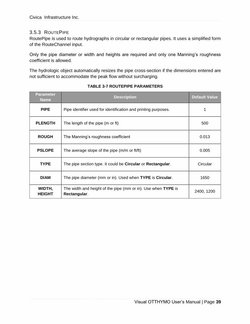
3.5.3 RoutePipe 39
3.5.4 RouteReservoir 40
3.5.5 ShiftHyd 40
3.6 Flow Separation Hydrologic Objects 41
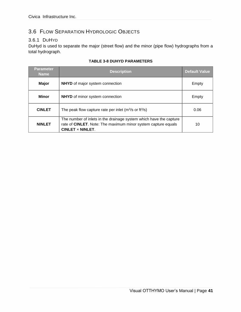
3.6.1 DuHyd 41
3.6.2 DivertHyd 42
3.7 Flow Merging Hydrologic Objects 43
3.8 Other Hydrological Objects 43
3.8.1 ReadHyd 43
3.8.2 StoreHyd 43
4 VISUAL OTTHYMO MAIN WINDOW 44
4.1 Overview 44
4.2 Toolbox 45
4.3 Toolbar 46
4.4 Project Manager 51
v
4.5 Properties 53
4.5.1 Editing Simple Property 54
4.5.2 Editing Collection Data 55
4.5.3 Editing LOSS Routine of StandHyd 56
4.5.4 CN* Flag 57
4.6 Parameter Tables 57
4.7 Hydrograph Results / Water Balance Results 59
4.8 Error List 60
5 WORKING WITH PROJECTS AND SCENARIOS 61
5.1 Projects 61
5.1.1 Project Types 61
5.1.2 Creating a New Project 61
5.1.3 Opening an Existing Project 62
5.1.4 Saving a Project 62
5.2 Scenarios 62
5.2.1 Creating a New Scenario 63
5.2.2 Duplicating an Existing Scenario 63
5.2.3 Opening an Existing Scenario 64
5.2.4 Setting Default Scenario 64
5.2.5 Scenario Settings 64
5.3 Importing Scenarios From Model Data Files 65
5.3.1 Model Data Files Supported 65
5.3.2 Importing SWMM5 65
5.3.3 Importing Visual OTTHYMO v2.4 and Later 66
5.3.4 Importing Visual OTTHYMO v2.0 - v2.3 Data Files 66
5.3.5 Importing Classic OTTHYMO Data Files 67
6 WORKING WITH CANVAS 69
6.1 Adding Background 69
6.2 Adding Hydrologic Objects 70
6.3 Selecting Hydrologic Objects 71
6.4 Changing the location of Hydrologic Objects 73

vi
6.5 Linking Hydrologic Objects 74
6.6 Navigating Canvas 75
6.7 Creating Labels 75
6.8 Printing Model Schematic 77
7 WORKING WITH THE MAP 78
7.1 Map View Layout 79
7.2 Default Coordinate System 80
7.3 Using Layers 80
7.3.1 Layer Types 80
7.3.2 Hydrologic Object Layers 81
7.3.3 Support Layers 82
7.3.4 Layer Context Menu 82
7.3.5 Adding a Layer 83
7.3.6 Moving Layers 84
7.3.7 Removing Layers 84
7.3.8 Defining Layer Visibility 84
7.3.9 Defining Layer Symbol 85
7.3.10 Labelling Layer 87
7.4 Using the Map 88
7.4.1 Navigating the Map 88
7.4.2 Selecting Features on Map 89
7.4.3 Creating Hydrologic Objects Manually 90
7.4.4 Creating Hydrologic Objects with GIS Data 92
7.4.5 Linking Hydrologic objects 93
7.4.6 Assigning Geometry to Existing Hydrological Objects 95
7.4.7 Moving, Editing and Deleting Hydrologic objects 96
7.4.8 Cutting Polygon-hydrologic objects 98
7.5 Updating Hydrologic objects Location in Schematic View 99
7.6 Using GIS Tools 100
7.6.1 Calculating CN 100
7.6.2 Calculating Area Weighted 102
7.6.3 Distributed Rainfall Modeling Technique (DRMT) 103
vii
7.7 Turning Off Map Functions 106
8 WORKING WITH CLIMATE LIBRARY 108
8.1 Opening Climate Library 108
8.2 Toolbar 109
8.3 Library Explorer 109
8.3.1 Oder of Items 109
8.3.2 Icons 111
8.3.3 Context Menu 111
8.3.4 Drag and Drop 111
8.4 Main View 112
8.5 Adding New Items 112
8.5.1 Adding Group 113
8.5.2 Adding IDF Group 113
8.5.3 Adding IDF Curve 115
8.5.4 Adding Design Storm 115
8.5.5 Adding Rain Gauge, Temperature Gauge and Evaporation Gauge 118
8.5.6 Adding Precipitation, Temperature and Evaporation Data 119
8.6 Assigning IDF to Chicago Design Storm 120
8.6.1 Coping and Pasting A, B, C 120
8.6.2 Dragging and Dropping IDF Curve to Chicago Design Storm 121
8.7 Sharing 121
8.7.1 Exporting 122
8.7.2 Importing 122
8.8 Adding Climate Data to Model 123
9 RUNING A SIMULATION 126
9.1 Overview 126
9.2 Single-event Simulation 126
9.3 Continuous Simulation 127
9.3.1 Setting Simulation Engine 127
9.3.2 Creating and Running Simulations 130
viii
10 WORKING WITH OUTPUT 132
10.1 Overview of Output Features 132
10.2 Single-event Simulation Outputs 133
10.2.1 Summary Data 133
10.2.2 Hydrograph Data 135
10.2.3 Hydrograph Plot 136
10.2.4 Traditional Detailed and Summary Output 140
10.2.5 Reviewing Output 142
10.3 Continuous Simulation Outputs 143
10.3.1 Summary Data 143
10.3.2 Time Series Plot 145
11 VISUAL OTTHYMO FILES 149
11.1 Project Files 149
11.2 Climate Data Files 149
11.3 Calibration Files 151
11.4 Hydrograph Files 152
12 TROUBLESHOOTING 154
12.1 Error and Warning Messages 154
12.1.1 Interface File Messages 154
12.1.2 Output File Messages 154
12.2 Program Quits During Run Simulation 156
Appendix A Parameter Edit Tools 157
A.1 Convert to CN* 157
A.2 Batch Assign 158
A.3 Calibrate Commands 160

Civica Infrastructure Inc.
Visual OTTHYMO User’s Manual | Page 1
1 INTRODUCTION
1.1 WELCOME
Welcome to Visual OTTHYMO v5.0 (VO5), the fifth version of the INTERHYMO-OTTHYMO hy-
drologic model simulation software package designed for Microsoft Windows OS.
OTTHYMO is a successful hydrologic management model that has been used for various simu-
lation analyses such as: Watershed Studies, Sub-watershed Studies, Master Drainage Plans,
Functional Stormwater Management Plans, Site Plans, and Stormwater Management Pond De-
signs.
1.2 WHAT’S NEW IN VERSION 5.0
With version 5.0, Visual OTTHYMO is extended from single-event simulation to continuous sim-
ulation to enable water balance analysis, erosion analysis and flow forecasting. Changes have
been made to adapt to continuous simulations as summarized below.
1. A new project type is added for continuous simulation. Existing single-event project could
be easily converted to a continuous project. With current version, the continuous model
supports five (5) hydrologic objects (NasHyd, StandHyd, AddHyd, RouteChannel and
RouteReservoir). Others will be added in later versions.
2. The Storm Library is extended to Climate Library. Long-term precipitation, temperature
and evaporation data could be added for continuous simulation.
3. The Project Manager is also extended to add temperature and evaporation data. Same
as the rainfall data, it’s added from the Climate Library and used in the simulation.
4. A Simulation Engine window is added for continuous simulation to change global settings
for the simulation run, e.g. snow melt base temperature. The simulate time step is also a
global parameter.
5. A new Batch Run window is created for continuous simulation. A simulation run will have
a name, a precipitation, the starting and ending time and optionally the temperature and
evaporation data.
6. The Hydrograph Results window is changed to Water Balance Results window for con-
tinuous simulation. The water balance components and peak flow is shown in the table.
7. The Water Balance menu is added to the canvas context menu to show the yearly and
monthly water balance summary.
8. The water balance summary results are available for labels in canvas.
9. The Plot Results button is added to Simulation tab to view the various time series data
with given time intervals.
10. Several single-event output tools, e.g. Summary Output, Detail Output, Cross Scenario
Plot, Hydrograph Result and Flow Data is removed for continuous simulation.

Civica Infrastructure Inc.
Visual OTTHYMO User’s Manual | Page 2
1.3 ABOUT THE USER’S MANUAL
The manual is divided into chapters and does not necessarily have to be read from start to finish.
Users that are familiar with previous releases of Visual OTTHYMO can probably learn how to
navigate around the model on their own and need only refer to the guide for new additional fea-
tures. The User’s Manual is organized as follows:
TABLE 1-1: USER’S MANUAL OUTLINE
Chapter Description
Chapter 1 - Introduction
This chapter gives an introduction to the model including new fea-
tures and how the Help System and documentation is organized,
how to install and uninstall the program.
Chapter 1 – Quick Start Tuto-
rial
This chapter provides a tutorial to help new users to understand the
basin steps to create and run a model.
Chapter 3 – Conceptual Model This chapter explains the conceptual model used in Visual OT-
THYMO and describes all hydrologic objects.
Chapter 4 – Visual OTTHYMO
Main Window
This chapter introduces the layout of the main interface and de-
scribes some of the windows.
Chapter 5 – Working with Pro-
jects and Scenarios
This chapter introduces the concept of project and scenario and de-
scribes how to manage them in Visual OTTHYMO.
Chapter 6 - Working with Can-
vas
This chapter describes the usage of the canvas to create a model in
Schematic View.
Chapter 7 – Working with the
Map
This chapter describes the usage of the map to create a model in
Map View.
Chapter 8 – Working with Cli-
mate Library
This chapter describes the concept and usage of Climate Library. It’s
the hub for climate data.
Chapter 9 – Running a Simu-
lation
This chapter guides users to change simulation engine parameter
and then create and run simulations.
Chapter 10 – Working with
Output
This chapter guides users to view simulation outputs with various
tools.
Chapter 11 – Visual OT-
THYMO Files
This chapter covers all the files used in Visual OTTHYMO including
importing from previous versions.
Chapter 12 - Troubleshooting This chapter guides users through some common troubleshooting sit-
uations.
1.4 VO HELP SUPPORT
VO has a comprehensive Help System and supporting documentation that will assist both begin-
ners as well as advanced users. One of the main goals in designing this Help System was to
empower the user with the tools and information so that almost every question could be answered
in a timely manner, without having to call for technical support. Should a question arise that is not
addressed in the user manual, please contact technical support at [email protected].
Civica Infrastructure Inc.
Visual OTTHYMO User’s Manual | Page 3
1.4.1 DOCUMENTATION
Two separate documents are accessible for VO, which include a User’s Manual and a Reference
Manual. This current document, the User’s Manual contains information on how to use the pro-
gram with a complete description of all the features. This manual does not concern the back-
ground theory. An online copy of the User’s Manual can be accessed online at http://visu-
alotthymo.com/downloads/v5.0_usermanual.pdf. The Reference Manual contains all of the hy-
drologic theory behind the program and gives guidance for users on how to select or measure
object parameter. The history of the development of the model is also addressed for advanced
users who need to know “why” and from “where”.
1.4.2 PROGRAM HELP FILE
To access the program’s help files, click the Help button at the top right corner or press F1.
You can use the Contents tab to jump to topics that tell you how to use VO, or to get quick access
to key reference topics.
1.4.3 HELP SEARCH
The fastest way to find a particular topic in Help is to use the Search dialog box (Index Tab). To
display the Search dialog box choose the Help Topics button on any Help topic screen and
choose the Index tab. To begin a search of the available topics (Index tab), type the first few
letters of the topic you are looking for, or make a selection from the list by scrolling up or down,
and then click Display. Alternatively, to search for a specific word in the Help topics, use the
Search tab. To begin a search for a specific word, type the first few letters of the word you are
looking for, or select matching words to narrow your search, and then choose one of the topics
where the word was found and click Display.
1.4.4 CONTEXT-SENSITIVE HELP (F1)
Many parts of VO are context-sensitive. Context-sensitive means you can get Help on these parts
directly without having to go through the Help menu. For example, to get Help on Climate Library
in VO, press F1 while Climate Library is opend. You can press F1 from any context-sensitive
part of the VO interface to display Help information about that part.
1.4.5 SEMINARS AND WORKSHOPS
Civica infrastructure Inc. (Civica Infrastructure) hosts seminars and workshops that allow the user
an opportunity to learn the basics of VO and to learn to use all its features to its full potential.
Seminars and workshops are organized by need. You can find more information from our website.
1.5 CUSTOMER SUPPORT
Users requiring support should first consult the User’s Manual and Reference Manual to try to
answer their question. Should a question not be addressed or further assistance is required, users
should contact Civica Infrastructure’s VO Technical Support [email protected] or +1 (905) 417-
9792. Live technical support is also available for all registered users regarding program installa-
tion and troubleshooting. Users requiring technical support pertaining to the use of the model in
an engineering application will be charged a nominal fee.
Civica Infrastructure Inc.
Visual OTTHYMO User’s Manual | Page 4
1.6 SOFTWARE LICENSE AGREEMENT
Before continuing with the installation and use of the Visual OTTHYMO™ software for stormwater
management, we suggest you read the following Software License Agreement and the inclusive
terms and conditions.
BY INSTALLING THE SOFTWARE, YOU ARE AGREEING TO BE BOUND BY THE TERMS
AND CONDITIONS OF THIS LICENSE. IF YOU DO NOT AGREE, DO NOT ACCEPT OR USE
THE SOFTWARE.
This End User License Agreement (“EULA”) is a legal agreement between you (either an individ-
ual or a single entity) and Civica Infrastructure Inc. (“Civica”) for access to the CIVICA software
application (“Software”) that accompanies this EULA, which may include associated media,
printed materials, “online” or electronic documentation, and Internet-based services.
GENERAL: CIVICA grants the user a license to use the Software under the terms and conditions
set forth in this EULA, provided that you comply with all such terms and conditions. The Software
is protected by copyright and other intellectual property laws and treaties. CIVICA owns the title,
copyright, and other intellectual property rights to the Software. CIVICA reserves all rights not
expressly granted to you in this EULA. The Software is licensed, not sold.
LICENSE: The software and the related documentation are licensed to you by Civica Infrastruc-
ture Inc. ("LICENSOR") as owner and also as distributor ("DISTRIBUTOR"). You will own the
media on which the Software is stored and provided to you herewith, but LICENSOR retains all
rights, including the copyright, in the Software and the related documentation. You may install
and maintain the Software (the "Installed Copy") on either a: (i) single computer for use by one
person at a time (without sharing); or (ii) network server for use on an internal network, provided
that the number of users concurrently using or sharing the Software does not exceed the number
of valid licenses of the Software you have purchased from the LICENSOR. You may not assign
or otherwise transfer any of your rights under this License to any third party. YOU AGREE TO
ENSURE THAT ANYONE WHO USES THE SOFTWARE DOES SO ONLY FOR YOUR AU-
THORIZED USE AND COMPLIES WITH THE TERMS OF THIS AGREEMENT.
TERM: This License is effective until terminated. You may terminate this License at any time by
destroying all copies (in any format and including the Installed Copy) of the Software and related
documentation. This License will terminate immediately, without notice from the LICENSOR, if
you fail to comply with any provision of this License. Upon termination, you must destroy all
copies (in any format and including the Installed Copy) of the Software and related documentation,
and you must notify LICENSOR in writing that all such copies have been destroyed.
RESTRICTIONS: The Software contains copyrighted material, trade secrets and other proprie-
tary material. Accordingly, YOU MUST NOT TRANSLATE, DECOMPILE, REVERSE ENGI-
NEER, DISASSEMBLE, MODIFY, ENHANCE, UPDATE, OR CREATE DERIVATIVE WORKS
BASED UPON OR INCORPORATING, THE SOFTWARE, IN WHOLE OR IN PART, UNLESS
AUTHORIZED IN WRITING BY LICENSOR. OTHER THAN AS EXPRESSLY PERMITTED
HEREIN, YOU MUST NOT USE OR COPY THE SOFTWARE OR RELATED DOCUMENTA-

Civica Infrastructure Inc.
Visual OTTHYMO User’s Manual | Page 5
TION. YOU MUST NOT NETWORK, RENT, LEASE, LOAN, OR DISTRIBUTE, THE SOFT-
WARE, IN WHOLE OR IN PART.
DISCLAIMER OF WARRANTY: You expressly acknowledge and agree that use of the Software
is at your sole risk. Although the SOFTWARE has been thoroughly tested and LICENSOR has
endeavored to make this program error free, the SOFTWARE is not and cannot be warranted as
infallible, and there remains the possibility of program errors. Further, the SOFTWARE is com-
plex, requiring professional engineering expertise and professional engineering judgment to input
information into the SOFTWARE and to interpret the information generated thereby. Therefore,
LICENSOR and DISTRIBUTOR can make no warranty either implicit or explicit as to the correct
performance or accuracy of the SOFTWARE to process or implement the information required.
THE SOFTWARE AND RELATED DOCUMENTATION ARE PROVIDED "AS IS" AND WITHOUT
WARRANTY OF ANY KIND, EXPRESSED OR IMPLIED, INCLUDING, BUT NOT LIMITED TO,
ANY IMPLIED WARRANTIES OF MERCHANTABILITY AND FITNESS FOR A PARTICULAR
PURPOSE. LICENSOR AND DISTRIBUTOR DO NOT WARRANT THAT THE SOFTWARE
WILL MEET YOUR REQUIREMENTS, OR THAT THE OPERATION OF THE SOFTWARE WILL
BE INTERRUPTED OR ERROR-FREE, OR THAT DEFECTS IN THE SOFTWARE WILL BE
CORRECTED. Furthermore, LICENSOR and DISTRIBUTOR do not warrant or make any repre-
sentations regarding the use or the results of the use of the Software or related materials in terms
of their correctness, accuracy, reliability or otherwise.
No oral or written information or advice given by LICENSOR or DISTRIBUTOR shall create a
warranty or in any way increase the scope of the warranty contained in this License.
CONFIDENTIALITY: “Confidential Information” means any information or data (including without
limitation any formula, pattern, compilation, program, device, method, technique, or process) that
is disclosed by one party (a “disclosing party”) to the other party (a “receiving party”) pursuant to
this Agreement. Confidential Information of CIVICA includes, but is not limited to, the terms of this
Agreement; the Software, as well as the structure, organization, design, algorithms, methods,
templates, data models, data structures, flow charts, logic flow, and screen displays associated
with such Software. Confidential Information does not include information that: (a) is or becomes
publicly known or available without breach of this Agreement; (b) is received by a receiving party
from a third party without breach of any obligation of confidentiality; or (c) was previously known
by the receiving party as shown by its written records.
A receiving party agrees: (a) to hold the disclosing party’s Confidential Information in strict confi-
dence; and (b) except as expressly authorized by this Agreement, not to, directly or indirectly,
use, disclose, copy, transfer or allow access to the Confidential Information. In addition, without
limiting the foregoing, CIVICA agrees to use, and to require its contractors to use, reasonable
procedures and mechanisms to maintain the security of and to prevent the unauthorized access
to the computer systems on which End User’s Confidential Information resides. Notwithstanding
the foregoing, a receiving party may disclose Confidential Information of the disclosing party as
required by law or court order; in such event, such party shall use its best efforts to inform the
other party prior to any such required disclosure.
Civica Infrastructure Inc.
Visual OTTHYMO User’s Manual | Page 6
SUBSCRIPTION: Upon the expiration of the initial one year subscription period, Licensee may
continue to receive access to the SOFTWARE and maintenance support for successive twelve
(12) month periods. The charge for such continual subscription fees shall be the LICENSOR’s
regular list price for the SOFTWARE as published from time to time by LICENSOR. Licensee shall
notify LICENSOR in writing its intent to receive optional maintenance. If Licensee fails to renew
optional maintenance and later elects to receive it, LICENSOR reserves the right to charge Licen-
see its subscription fees for the period(s) of the lapsed maintenance. Should the Licensee allow
a lapse in maintenance, the Licensee forfeits access to technical support, updates and upgrades
that may be available for the SOFTWARE. LICENSOR may elect to discontinue maintenance at
any time upon written notice to Licensee.
MEDIA WARRANTY: LICENSOR warrants that the software provided to you by LICENSOR on
which the Software is stored, shall be free from defects in materials and workmanship under nor-
mal use for ninety (90) days from the date of delivery to you.
LIMITATION OF LIABILITY: UNDER NO CIRCUMSTANCES, INCLUDING NEGLIGENCE,
SHALL LICENSOR OR DISTRIBUTOR BE LIABLE TO YOU OR ANY OTHER PARTY FOR ANY
INCIDENTAL, SPECIAL OR CONSEQUENTIAL DAMAGES THAT RESULT FROM THE USE
OR INABILITY TO USE THE SOFTWARE OR RELATED DOCUMENTATION, EVEN IF LICEN-
SOR OR DISTRIBUTOR HAVE BEEN ADVISED OF THE POSSIBILITY OF SUCH DAMAGES.
IN NO EVENT SHALL LICENSOR'S OR DISTRIBUTOR'S TOTAL LIABILITY TO YOU FOR ALL
DAMAGES, LOSSES, AND CAUSES OF ACTION (WHETHER IN CONTRACT, TORT (INCLUD-
ING NEGLIGENCE) OR OTHERWISE) EXCEED THE AMOUNT PAID TO LICENSOR OR DIS-
TRIBUTOR TO LICENSE THE SOFTWARE HEREUNDER.
CONTROLLING LAW AND SEVERABILITY: This License shall be governed by and construed
in accordance with the laws of the province of Ontario and adjudicated in a court of that province.
If, for any reason, a court of competent jurisdiction finds any provision of the License, or portion
thereof, to be unenforceable, that provision of the License shall be enforced to the maximum
extent permissible in order to affect the intention of the parties, and the remainder of this License
shall continue in full force and effect.
INDEMNIFICATION: If a claim of copyright, patent, trade secret, or other intellectual property
rights violation is made against End User relating to the Software, End User agrees to immediately
notify CIVICA, allow CIVICA to control the litigation or settlement of such claim, and cooperate
with CIVICA in the investigation, defense, and/or settlement thereof. CIVICA agrees to take con-
trol of the litigation and indemnify the End User by paying any settlement approved by CIVICA, or
any judgment, costs, or attorneys’ fees finally awarded against the End User for such claim. End
User may participate at End User’s own expense. This indemnification obligation does not apply
to the extent the claim is based on a combination of Software with other software, or any modifi-
cation to the Software, if such claim would not have been made but for the combination or modi-
fication. If such a claim is made or, in CIVICA’s opinion, is likely to be made, CIVICA, at its sole
discretion, may modify the Software, obtain rights for the End User to continue using the Software,
or terminate the agreement for the Software.
THIRD PARTY SOFTWARE: Visual OTTHYMO Software may include software under license
Civica Infrastructure Inc.
Visual OTTHYMO User’s Manual | Page 7
from third parties (“Third Party Software” and “Third Party License”). Any Third-Party Software is
licensed to you is subject to the terms and conditions of the corresponding Third-Party License.
The Third-Party License(s) is located in the license.txt file. Please contact Visual OTTHYMO sup-
port if you cannot find a Third-Party License.
MISCELLANEOUS: Neither party shall be liable for any failure or delay in the performance of its
obligations due to causes beyond the reasonable control of the party affected, including but not
limited to war, sabotage, insurrection, riot or other act of civil disobedience, strikes or other labor
shortages, act of any government affecting the terms hereof, accident, fire, explosion, flood, hur-
ricane, severe weather or other act of God.
TECHNICAL SUPPORT: CIVICA shall provide e-mail technical and phone support to the End
User. CIVICA will attempt to respond to e-mail requests for technical support within one business
day (24 hours); phone response within working hours, 9am to 5pm. Monday thru Friday (excluding
public Canadian Holidays) Eastern Standard Time (EST).
PRIVACY POLICY: CIVICA protects your data. View CIVICA’s Privacy Policy online at this link
COMPLETE AGREEMENT: This License constitutes the entire agreement between the parties
with respect to the use of the Software and related materials, and supersedes all prior or contem-
poraneous understandings or agreements, written or oral, regarding such subject matter.
ACCEPTANCE: Acceptance of this license is deemed to have occurred by the instillation and
use of the software.
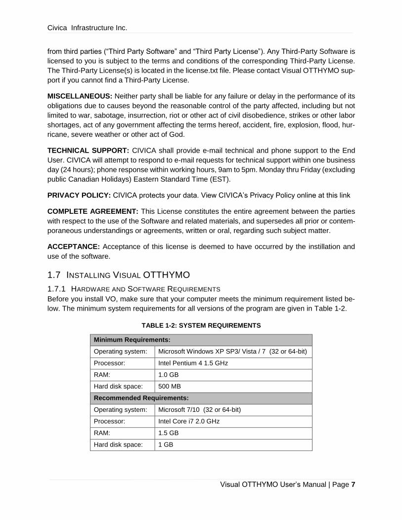
1.7 INSTALLING VISUAL OTTHYMO
1.7.1 HARDWARE AND SOFTWARE REQUIREMENTS
Before you install VO, make sure that your computer meets the minimum requirement listed be-
low. The minimum system requirements for all versions of the program are given in Table 1-2.
TABLE 1-2: SYSTEM REQUIREMENTS
Minimum Requirements:
Operating system: Microsoft Windows XP SP3/ Vista / 7 (32 or 64-bit)
Processor: Intel Pentium 4 1.5 GHz
RAM: 1.0 GB
Hard disk space: 500 MB
Recommended Requirements:
Operating system: Microsoft 7/10 (32 or 64-bit)
Processor: Intel Core i7 2.0 GHz
RAM: 1.5 GB
Hard disk space: 1 GB

Civica Infrastructure Inc.
Visual OTTHYMO User’s Manual | Page 8
1.7.2 LICENSING SYSTEM
VO has a simple yet effective cloud-based licensing protection system to ensure that users com-
ply with the terms of their license agreement. As set out in the license agreement, VO may be
installed in multiple computers, but only the computer securing an license from cloud will be able
to run the application.
A customer portal is provided to track the usage of all licenses. For more information, please refer
to Customer Portal for Cloud-based Licensing.
1.7.3 INSTALLATION VO
Before installing VO, make sure that you have closed all other programs and that any virus pro-
tection software is disabled. To install VO on your computer, please follow the directions below.
Step 1: Download the installation file from VO Download page. The download link is updated
once a new version is available.
Step 2: Click on the installation file and follow the instructions in the installation wizard as
seen below.
Step 3: Accept the License Agreement

Civica Infrastructure Inc.
Visual OTTHYMO User’s Manual | Page 9
Step 4: By default, VO5 is installed on C:\Program Files (x86)\Visual OTTHYMO 5.0
Step 5: Setup will create a shortcut in the Start Menu folder
Step 6: Choose to Create a Desktop Icon AND UNCHECK USB Key License driver as we
now utilize a cloud based licensing system.
Civica Infrastructure Inc.
Visual OTTHYMO User’s Manual | Page 10
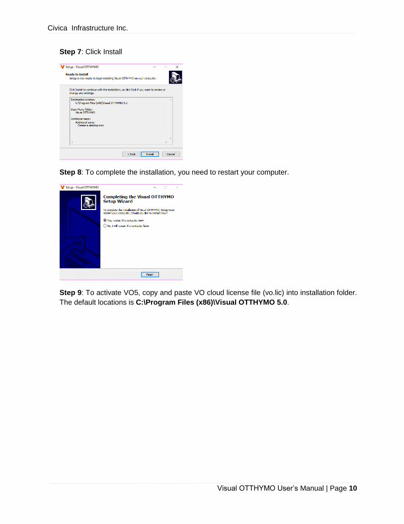
Step 7: Click Install
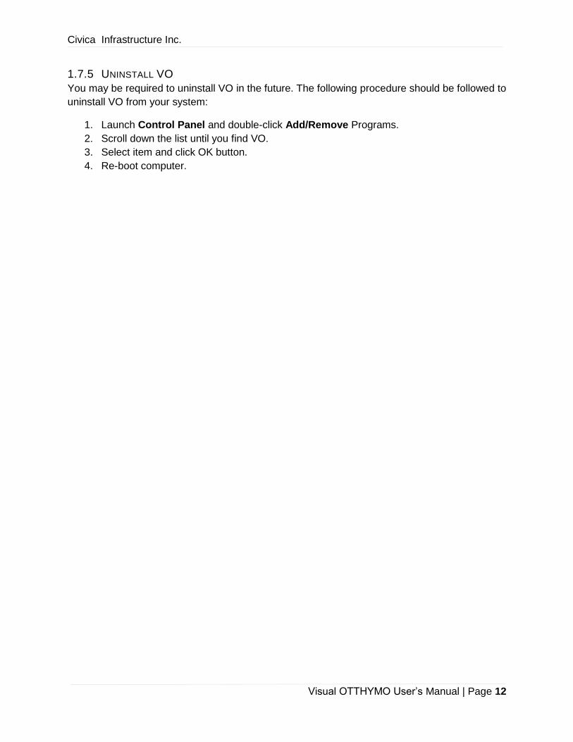
Step 8: To complete the installation, you need to restart your computer.
Step 9: To activate VO5, copy and paste VO cloud license file (vo.lic) into installation folder.
The default locations is C:\Program Files (x86)\Visual OTTHYMO 5.0.

Civica Infrastructure Inc.
Visual OTTHYMO User’s Manual | Page 11
1.7.4 RUNNING VO
To start VO, simply double-click on the VO desktop icon or find the VO item from your Start
menu. Once VO starts, you will first see the splash screen (Figure 1-1) and then the main window
(Figure 1-2).
FIGURE 1-1 VISUAL OTTHYMO SPLASH SCREEN
FIGURE 1-2 VISUAL OTTHYMO MAIN WINDOW
Civica Infrastructure Inc.
Visual OTTHYMO User’s Manual | Page 12
1.7.5 UNINSTALL VO
You may be required to uninstall VO in the future. The following procedure should be followed to
uninstall VO from your system:
1. Launch Control Panel and double-click Add/Remove Programs.
2. Scroll down the list until you find VO.
3. Select item and click OK button.
4. Re-boot computer.

Civica Infrastructure Inc.
Visual OTTHYMO User’s Manual | Page 13
2 QUICK START TUTORIAL
This Chapter provides a tutorial on how to use Visual OTTHYMO. By following along with this
chapter, you can quickly learn about the steps involved in building a model.
2.1 EXAMPLE STUDY AREA
In this tutorial, we will create a single-event VO model for the watershed shown below. It has two
urban catchments (1003 and 1005) and three rural catchments (1001, 1002 and 1004). Then we
will run the simulation with 2-100yr design storms. The model is then converted to a continuous
model and run the simulation with 10-year precipitation and temperature data.
FIGURE 2-1 EXAMPLE STUDY AREA
2.2 PROJECT SETUP FOR SIGLE-EVENT MODEL
To create a single-event OTTHYMO project, select File -> New Project -> New Otthymo Pro-
ject.
FIGURE 2-2 NEW OTTHYMO PROJECT MENU
To have a reference to place the hydrologic objects, a background picture could be added to the
canvas. To add the background, switch to Schematic View and choose Background -> Change
Background… from the context menu. Change the position of the background with mouse.

Civica Infrastructure Inc.
Visual OTTHYMO User’s Manual | Page 14
FIGURE 2-3 BACKGROUND IN CANVAS
2.3 CREATING DRAINAGE NETWORK ON CANVAS
All available hydrologic objects are list in Tool Box on the left. To add one hydrologic object on
canvas in Schematic View, drag and drop it on canvas. Then it can be moved to any location.
FIGURE 2-4 ADDING HYDROLOGIC OBJECTS TO CANVA
The study area has two urban catchments, three rural catchments, three channels and two con-
fluence points. They could be modeled with StandHyd , NasHyd , RouteChannel and
AddHyd respectively. Drag and drop them from Tool Box to Canvas and move them to the
proper location based on the background. At this point your canvas should look like the one shown

Civica Infrastructure Inc.
Visual OTTHYMO User’s Manual | Page 15
below. Note that the ID of each command is labeled at the bottom and few hydrologic object icons
have red outlines indicating errors.
FIGURE 2-5 SINGLE-EVENT MODEL BEFORE ALL HYDROLOGIC OBJECTS ARE CONNECTED
Then the drainage system components (hydrologic objects) will be connected to form a connected
system. The connection between hydrologic objects tells where the flow come from and where
the flow will go. On canvas. it’s represented by an arrow line pointing from the source to the
destination.
In the example study area, the flow generated at catchment 1003 flows to channel 2002. The
relationship is represented by a connection (or link) from StandHyd 1003 to RouteChannel 2002.
To create this connection, move the cursor on top of the 1003. Notice that the curve changes to
a cross. Then hold the left mouse button, move to 2002 and release the left mouse button.
The connection between other hydrologic objects could also be created. At this point your canvas
should look like that shown below. Note that the red outline disappears
Civica Infrastructure Inc.
Visual OTTHYMO User’s Manual | Page 16
FIGURE 2-6 SAMPLE SINGLE-EVENT MODEL
2.4 SETTING HYDROLOGIC OBJECT PROPERTIES
Default parameter values are used for newly created hydrologic objects, which may need to be
changed to represent the working project. Parameters could be edited with the Properties win-
dow or the Parameters Tables window.
The Properties window is used to edit the parameters of selected objects. If more than one ob-
jects are selected, only the common parameters are editable and changes will be applied to all
selected objects.
The Parameter Tables windows shows all parameters of each type of objects in a table. The
table could be sorted by any columns. Besides editing single parameter value, data could be
copied from a spreadsheet software as along as the columns are in the same order.
To edit the value for a property, select the hydrologic object(s) on the canvas and find the property
in Properties window or Parameter Tables window. Type in the new value in the text box or
select proper options from the combo box.

Civica Infrastructure Inc.
Visual OTTHYMO User’s Manual | Page 17
FIGURE 2-7 PARAMETER TABLES AND PROPERTIES WINDOW
2.5 ADDING DESIGN STORM
The design storm is added from Climate Library to Project Manager and then used in the sim-
ulation.
Climate Library
The Climate Library is a library of climate data including design storm and long-term measured
precipitation data. The climate data for the model simulation should be first added to the Climate
Library before it could be used in model simulation.
To open the Climate Library, click Climate Library button in Simulation tab. Some design
storms and reginal storms used in TRCA are shipped with VO, which could be good starting point.
If the required climate data is not available in the library, it could be added from different sources.
Properties
Parameter Tables
Civica Infrastructure Inc.
Visual OTTHYMO User’s Manual | Page 18
FIGURE 2-8 CLIMATE LIBRARY WITH DESIGN STORM
Project Manager
Project Manager is where the scenarios and climate data is managed. It’s located at the right
side of the main window.
FIGURE 2-9 PROJECT MANAGER FOR SINGLE-EVENT MODEL
Adding Design Storm from Climate Library to Project Manager
To add a design storm to the project, drag and drop the design storm node from Library Explorer
to the Rain Data section in Project Manager. A new rain group will be added in Project Manager.
Design storms for other return period could be added with the same method. Note that design
storms of different return periods should be added to different rain groups.
Civica Infrastructure Inc.
Visual OTTHYMO User’s Manual | Page 19
FIGURE 2-10 ADDING DESIGN STROM FROM CLIMATE LIBRARY TO PROJECT MANAGER
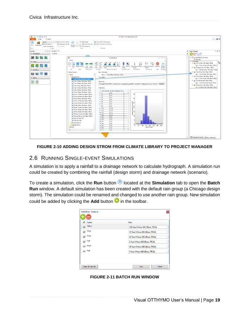
2.6 RUNNING SINGLE-EVENT SIMULATIONS
A simulation is to apply a rainfall to a drainage network to calculate hydrograph. A simulation run
could be created by combining the rainfall (design storm) and drainage network (scenario).
To create a simulation, click the Run button located at the Simulation tab to open the Batch
Run window. A default simulation has been created with the default rain group (a Chicago design
storm). The simulation could be renamed and changed to use another rain group. New simulation
could be added by clicking the Add button in the toolbar.
FIGURE 2-11 BATCH RUN WINDOW

Civica Infrastructure Inc.
Visual OTTHYMO User’s Manual | Page 20
To run simulations, check the simulations in the first column and then click the Run button at the
bottom. A window will appear to show the simulation run progress. The Batch Run window will
be closed after the simulation run is finished.
2.7 VIEWING SINGLE-EVENT SIMULATION OUTPUTS
The main output from a single-event simulation is hydrograph. The hydrographs could be dis-
played in graph, table and summary.
Graph
To plot hydrographs with rainfall, select the hydrologic objects and then click the Hydrograph
button in Simulation tab. The Hydrograph window will appear. The appearance of the plot
could be changed using the control panel on the left.
FIGURE 2-12 HDYROGRAPH WINDOW
Table
To view the hydrograph data in a table, click the Flow Data button in Simulation tab. The data
could be exported to a file.
FIGURE 2-13 HYDROGRAPH FLOW DATA

Civica Infrastructure Inc.
Visual OTTHYMO User’s Manual | Page 21
Summary
The summary of a hydrograph includes drainage area (AREA), peak flow (PKFW), time to peak
(TP), runoff volume (RV) and dry weather flow (DWF). To view the summary of all hydrographs,
use the Hydrograph Result window located at the bottom.
FIGURE 2-14 HYDROGRAPH RESULTS WINDOW
The summaries could be labeled on canvas besides the hydrologic objects as shown in Figure
2-15.
FIGURE 2-15 HYDROGRAPH SUMMARY LABEL
Text
The classic OTTHYMO detail and summary output is available through the Detail Output and
Summary Output button.
FIGURE 2-16 DETAIL OUTPUT (TEXT)

Civica Infrastructure Inc.
Visual OTTHYMO User’s Manual | Page 22
FIGURE 2-17 SUMMARY OUTPUT (TEXT)
2.8 CONVERTING TO CONTINUOUS OTTHYMO MODEL
The single-event OTTHYMO model could be convert to continuous OTTHYMO model to run con-
tinuous simulation. To do this, first create a Continuous OTTHYMO project using menu File ->
New Project -> New Continuous Otthymo Project.
FIGURE 2-18 NEW CONTINUOUS OTTHYMO PROJECT MENU
Then the single-event model could be imported to the Continuous project using the menu File ->
Import -> Import VH Scenario (Current Project). Extra parameters (e.g. land cover and soil
parameters) are added to hydrologic objects to enable continuous simulation.
FIGURE 2-19 IMPORT VH SCENARIO (CURRENT PROJECT) MENU

Civica Infrastructure Inc.
Visual OTTHYMO User’s Manual | Page 23
2.9 ADDING LONG-TERM PRECIPITATION AND TEMPERATURE
Same as design storm, long-term precipitation and temperature could be added from Climate
Library to Project Manager by drag-and-drop.
FIGURE 2-20 ADDING TEMPERATURE DATA FROM CLIMATE LIBRARY TO PROJECT MANAGER
2.10 RUNNING CONTINUOUS SIMULATIONS
Besides rainfall data, a continuous simulation could also use temperature and evaporation data.
It’s also required to setup the starting and ending date.
To create a continuous simulation, click the Run button located at the Simulation tab to open
the Batch Run window. And then click the Add button in the toolbar to create a simulation. If
precipitation and/or temperature is available in Project Manager, it will be automatically selected
in the new simulation. The starting and ending date is also automatically based on the precipita-
tion and temperature data.
To run simulations, check the simulations in the first column and then click the Run button at the
bottom. A window will appear to show the simulation run progress. The Batch Run window will
be closed after the simulation run is finished.

Civica Infrastructure Inc.
Visual OTTHYMO User’s Manual | Page 24
FIGURE 2-21 BATCH RUN WINDOW FOR CONTINUOUS SIMULATION
Note that the default time step for a continuous simulation is 5 minutes. The simulation run may
take a while when the climate data covers long time period. To use a longer time step, change it
in the Simulation Engine window (Engine Options button in Simulation tab).
FIGURE 2-22 SIMULATION TIME STEP SETTING IN SIMULATING ENGINE WINDOW
2.11 VIEWING CONTINUOUS SIMULATION OUTPUTS
The continuous simulation models the water balance in snow pack and active soil zone. All the
water balance components are available as time-series data from the outputs. Similar with hydro-
graph summary, these water balance components are also summarized to help get the big pic-
ture.
Time Series
There are two days to plot the time series data. The Hydrograph button is similar with the one
for single-event simulation, which will open the Hydrograph window plotting flow versus precipi-
tation.

Civica Infrastructure Inc.
Visual OTTHYMO User’s Manual | Page 25
FIGURE 2-23 HYDROGRAPH WINDOW FOR CONTINUOUS SIMULATION
Another tool is Plot Results , which will plot all available water balance components from a
hydrological object. The time series data could be plotted with the original time interval or with
higher ones (year, month and week).
FIGURE 2-24 PLOT RESULT WINDOW FRO CONTINUOUS SIMULATION

Civica Infrastructure Inc.
Visual OTTHYMO User’s Manual | Page 26
Summary
The average annual summary of the water balance components is shown in the Water Balance
Results window located at the bottom.
FIGURE 2-25 WATER BALANCE RESULTS FOR CONTINUES SIMULATION
To view the yearly and monthly summary for each catchment, choose Water Balance from the
canvas context menu. The Water Balance window will appear.
FIGURE 2-26 WATER BALANCE WINDOW FOR CONTINUOUS SIMULATION

Civica Infrastructure Inc.
Visual OTTHYMO User’s Manual | Page 27
The average annual summaries could also be labeled on canvas.
FIGURE 2-27 WATER BALANCE SUMMARY LABEL

Civica Infrastructure Inc.
Visual OTTHYMO User’s Manual | Page 28
3 CONCEPTUAL MODEL
3.1 INTRODUCTION
Visual OTTHYMO models flows generated from rainfall (or snow melt) on a drainage system. The
drainage system first receive water from rainfall or snow melt and transform it to flow. The flow is
then routed from upstream to the outlet. Structures may exist to 1) merge multiple flows together
or 2) split one single flow to multiple parts.
Visual OTTHYMO conceptualized the drainage system as a collection of hydrologic processes. A
hydrologic process is a unit process to 1) generate flow from rainfall, 2) route flow, 3) merge flow
or 4) split flow. Each hydrologic process is modeled with a Hydrologic Object, a visual object
represented with an icon on canvas or a feature on map. The hydrologic objects are then con-
nected to simulate the sequence of hydrologic processes to simulate the whole drainage system.
FIGURE 3-1 THE CONCEPTUAL MODEL OF VISUAL OTTHYMO
An example of the conceptual model is given in Figure 3-1. The drainage system consists of five
(5) catchments, three (3) channels and two (2) confluence points. The system could be broken
(1) (2)
(3) (4)

Civica Infrastructure Inc.
Visual OTTHYMO User’s Manual | Page 29
down to five catchments, three channels and two confluence points where catchments transform
the rainfall to flow, channels route flow and confluence points merge flow. Each of the components
is a hydrologic process and could be represented with a Hydrologic Object (the icon at the right
bottom corner of each component). The drainage system could be simulated with these hydrologic
objects in Visual OTTHYMO by creating the hydrologic objects first and then linking them as a
connected system.
The behavior of a hydrologic process (e.g. flow generation) may be different. The behavior could
be characterized with parameters (e.g. area and slope) and algorithms (e.g. different unit hydro-
graph). Visual OTTHYMO use a different Hydrologic Object for different algorithms of same
hydrologic process. For example, the flow from a catchment could be calculated using the Nash
unit hydrograph or William unit hydrograph. So two different types of hydrologic objects, NasHyd
and WilHyd, are provided in Visual OTTHYMO. As different algorithms may require different pa-
rameters, the parameters of different hydrologic objects will also be different.
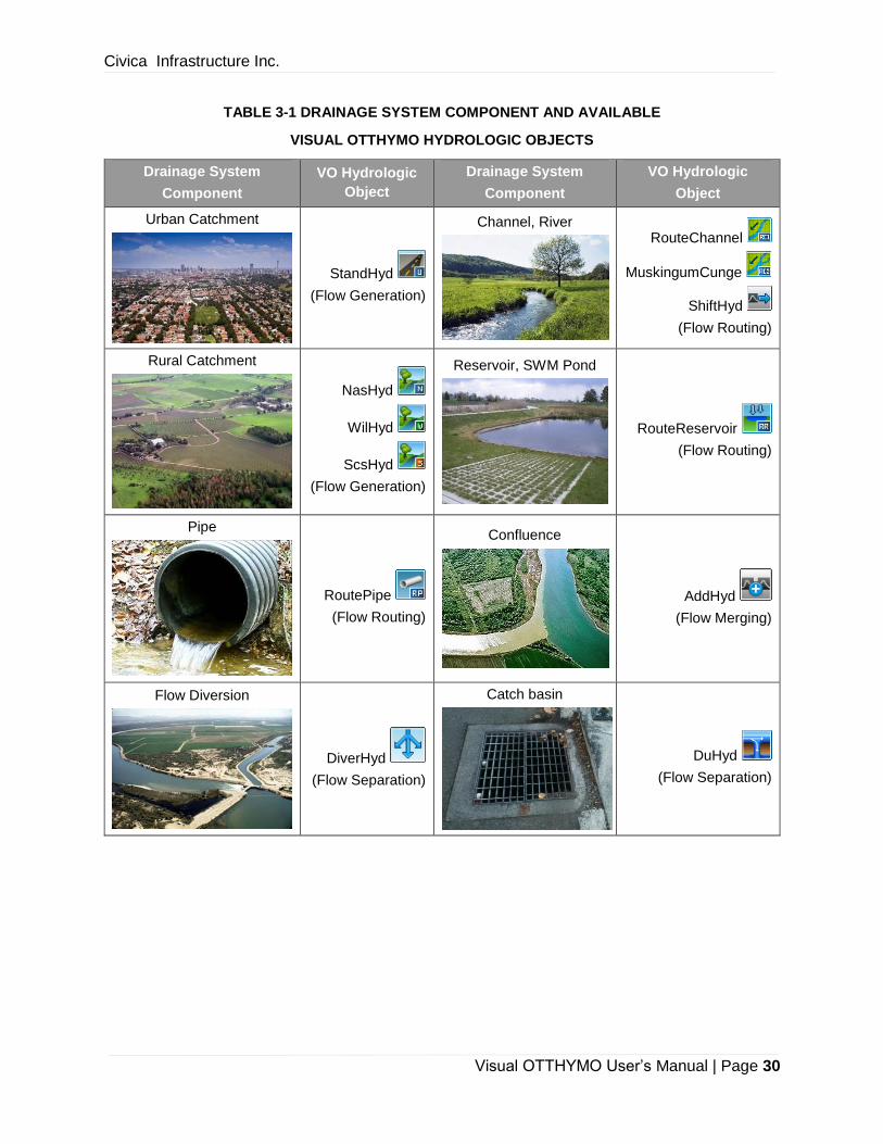
3.2 VISUAL OTTHYMO HYDROLOGIC OBJECTS OVERVIEW
The drainage system component and the corresponding Visual OTTHYMO hydrologic objects are
list in Table 3-1. The hydrologic process modelled is also given below each hydrologic object,
which are 1) flow generation, 2) flow routing, 3) flow separation and 4) flow merging. Each hydro-
logic object is represented with an unique icon.
Flow generation process generates flow from rainfall or snow melt. It happens on catchments.
Flow from a rural catchment and an urban catchment is quite different due to decreased infiltration
caused by urbanization. With same amount of rainfall, the hydrograph from an urban catchment
has larger and earlier peak flow and more runoff volume. Visual OTTHYMO provides one hydro-
logic object for urban catchments and three hydrologic objects for rural catchments. Often rural
hydrologic objects in existing condition needs to be converted to urban hydrologic objects for post-
development condition.
Flow routing process route flow through a certain structure. The hydrograph is usually changed
(delay and attenuation). The structures supported are channels, reservoirs (ponds) and pipes.
Ponds are important as it’s usually required for a new development to control the flow to the
allowable rates. Visual OTTHYMO can help size the ponds by determining the rating curve (stor-
age-discharge relationship).
Flow separation separates flow to multiple receiving structures. It happens at flow diversion or
catch basins. The latter is commonly used in new developments to have part of the runoff flow
into the sewer system. In planning stage, the number of catch basins could be estimated and
Visual OTTHYMO can model it with minimal parameters.
Flow merging merges flow from different sources to one single flow. It usually happens at the
confluence points. The outlet of the study area is usually a confluence point.
Civica Infrastructure Inc.
Visual OTTHYMO User’s Manual | Page 30
TABLE 3-1 DRAINAGE SYSTEM COMPONENT AND AVAILABLE
VISUAL OTTHYMO HYDROLOGIC OBJECTS
Drainage System
Component
VO Hydrologic
Object
Drainage System
Component
VO Hydrologic
Object
Urban Catchment
StandHyd
(Flow Generation)
Channel, River
RouteChannel
MuskingumCunge
ShiftHyd
(Flow Routing)
Rural Catchment
NasHyd
WilHyd
ScsHyd
(Flow Generation)
Reservoir, SWM Pond
RouteReservoir
(Flow Routing)
Pipe
RoutePipe
(Flow Routing)
Confluence
AddHyd
(Flow Merging)
Flow Diversion
DiverHyd
(Flow Separation)
Catch basin
DuHyd
(Flow Separation)
Civica Infrastructure Inc.
Visual OTTHYMO User’s Manual | Page 31
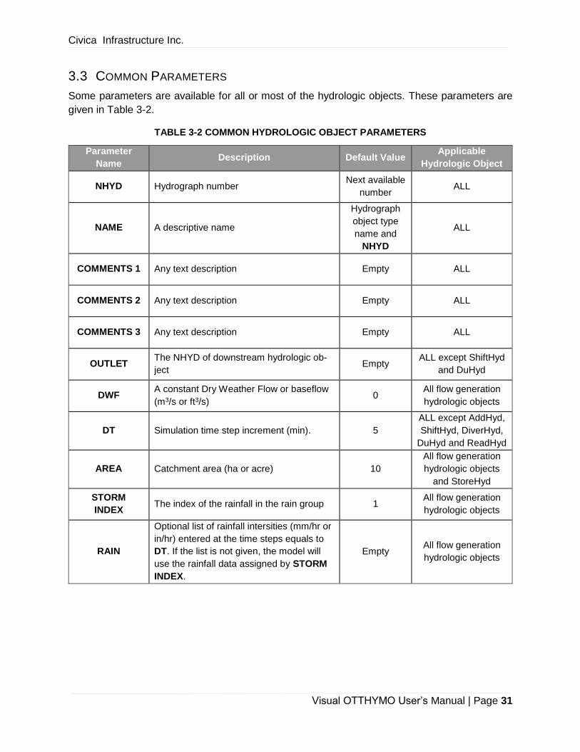
3.3 COMMON PARAMETERS
Some parameters are available for all or most of the hydrologic objects. These parameters are
given in Table 3-2.
TABLE 3-2 COMMON HYDROLOGIC OBJECT PARAMETERS
Parameter
Name Description Default Value
Applicable
Hydrologic Object
NHYD Hydrograph number Next available
number ALL
NAME A descriptive name
Hydrograph
object type
name and
NHYD
ALL
COMMENTS 1 Any text description Empty ALL
COMMENTS 2 Any text description Empty ALL
COMMENTS 3 Any text description Empty ALL
OUTLET The NHYD of downstream hydrologic ob-
ject Empty
ALL except ShiftHyd
and DuHyd
DWF A constant Dry Weather Flow or baseflow
(m3/s or ft3/s) 0
All flow generation
hydrologic objects
DT Simulation time step increment (min). 5
ALL except AddHyd,
ShiftHyd, DiverHyd,
DuHyd and ReadHyd
AREA Catchment area (ha or acre) 10
All flow generation
hydrologic objects
and StoreHyd
STORM
INDEX The index of the rainfall in the rain group 1
All flow generation
hydrologic objects
RAIN
Optional list of rainfall intersities (mm/hr or
in/hr) entered at the time steps equals to
DT. If the list is not given, the model will
use the rainfall data assigned by STORM
INDEX.
Empty All flow generation
hydrologic objects
Civica Infrastructure Inc.
Visual OTTHYMO User’s Manual | Page 32
3.4 FLOW GENERATION HYDROLOGIC OBJECTS
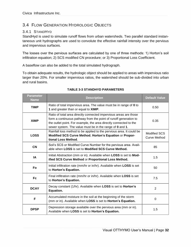
3.4.1 STANDHYD
StandHyd is used to simulate runoff flows from urban watersheds. Two parallel standard instan-
taneous unit hydrographs are used to convolute the effective rainfall intensity over the pervious
and impervious surfaces.
The losses over the pervious surfaces are calculated by one of three methods: 1) Horton’s soil
infiltration equation; 2) SCS modified CN procedure; or 3) Proportional Loss Coefficient.
A baseflow can also be added to the total simulated hydrograph.
To obtain adequate results, the hydrologic object should be applied to areas with impervious ratio
larger than 20%. For smaller impervious ratios, the watershed should be sub-divided into urban
and rural basins.
TABLE 3-3 STANDHYD PARAMETERS
Parameter
Name Description Default Value
TIMP Ratio of total impervious area. The value must be in range of 0 to
1 and greater than or equal to XIMP. 0.50
XIMP
Ratio of total area directly connected impervious areas are those
form a continuous pathway from the point of runoff generation to
the outlet point. For example, the area directly connected to the
sewer system. The value must be in the range of 0 and 1.
0.35
LOSS
Rainfall loss method to be applied to the pervious area. It could be
Modified SCS Curve Method, Horton’s Equation or Propor-
tional Loss Method.
Modified SCS
Curve Method
CN Soil’s SCS or Modified Curve Number for the pervious area. Avail-
able when LOSS is set to Modified SCS Curve Method. 85
IA Initial Abstraction (mm or in). Available when LOSS is set to Mod-
ified SCS Curve Method or Proportional Loss Method. 1.5
Fo Initial infiltration rate (mm/hr or in/hr). Available when LOSS is set
to Horton’s Equation. 50
Fc Final infiltration rate (mm/hr or in/hr). Available when LOSS is set
to Horton’s Equation. 7.5
DCAY Decay constant (1/hr). Available when LOSS is set to Horton’s
Equation. 2
F Accumulated moisture in the soil at the beginning of the storm
(mm or in). Available when LOSS is set to Horton’s Equation. 0
DPSP Depression storage available over the pervious area (mm or in).
Available when LOSS is set to Horton’s Equation. 1.5

Civica Infrastructure Inc.
Visual OTTHYMO User’s Manual | Page 33
Parameter
Name Description Default Value
C Proportional loss coefficient ration (between 0 and 1). Available
when LOSS is set to Proportional Loss Method. 0.5
SLPP Average slope of the pervious area (%). Value must be greater
than 0.0. 2
LGP Overland flow length of the pervious area (m or ft) 40
MNP
Manning’s roughness coefficient for pervious surfaces. Note that
coefficient should be selected based on sheet flow, not channel
flow.
0.25
SCP Storage coefficient for the linear reservoir of the pervious area
(hr). Enter 0 to allow the program to internally select the value. 0
DPSI Available depression storage over the impervious area (mm or in). 1
SLPI Average slope of impervious area (%) 1
LGI Type
LGI calculation method. It could be Auto and Manual. Auto will
calculate the LGI from AREA assuming AREA = 1.5(LGI)2. Man-
ual will read the LGI value from user input.
Auto
LGI The overland flow length of impervious area (m or ft) Calculated from
AREA
MNI
Manning’s roughness coefficient for pervious surfaces. Note that
coefficient should be selected based on channel flow (i.e. sewer
and/or road flow).
0.013
SCI Storage coefficient for the linear reservoir of the impervious area
(hr). Enter 0 to allow the program to internally select the value. 0

Civica Infrastructure Inc.
Visual OTTHYMO User’s Manual | Page 34
3.4.2 NASHYD
NasHyd is used to simulate runoff flows with Nash instantaneous unit hydrograph. This hydro-
graph is made of cascade of “N” linear reservoirs. The command is mainly used for rural areas
but can also be used for very large urban watersheds and to simulate the effects of infiltration/in-
flow in sanitary sewers. Rainfall losses can be computed by a SCS modified CN procedure or
Proportional Loss Coefficient.
TABLE 3-4 NASHYD PARAMETERS
Parameter
Name Description
Default
Value
CN SCS Modified Curve Number or Proportional Loss Coefficient (if
negative value between 0 and -1 entered). 80
IA
Initial abstraction (mm or in). If IA is negative, the program uses the
SCS method where IA = 0.2 × S and S is a function of Curve Num-
ber.
5
N Number of linear reservoir used for the derivations of Nash Unit Hy-
drograph. 3
TP Unit Hydrograph time to peak (hr). It is approximately equal to (N-
1)/N × TC where TC is the Time of Concentration. 0.2

Civica Infrastructure Inc.
Visual OTTHYMO User’s Manual | Page 35
3.4.3 WILHYD
WilHyd is used to Simulate hydrographs from rural watersheds with long recession periods. The
program uses the Williams and Hann’s unit hydrographs developed in the original HYMO program
and the modified SCS Curve Number procedure to calculate the rainfall losses.
TABLE 3-5 WILHYD PARAMETERS
Parameter
Name Description
Default
Value
AA/DWF
Printout parameter or if less than 0, to enter a constant Dry Weather
Flow or baseflow (m3/s or ft3/s). If AA is positive, the unit hydrograph
will be printed. If AA is 0, neither happens.
0
BB Printout parameter. If BB is positive the rainfall excess ordinates will
be printed. If BB is 0, excess ordinates will not be printed. 3
CN SCS Modified Curve Number 80
IA
Initial abstraction (mm or in). If IA is negative, the program uses the
SCS method where IA = 0.2 × S and S is a function of Curve Num-
ber.
5
K Recession constant in the William and Hann unit hydrograph equa-
tion (hr) 4
TP Unit hydrograph time to peak (hr). The time step DT should be
smaller than TP. 0.2

Civica Infrastructure Inc.
Visual OTTHYMO User’s Manual | Page 36
3.4.4 SCSHYD
ScsHyd is essentially the same as the NasHyd with exception that it uses parameters for the SCS
procedure (i.e. initial abstraction is a function of the SCS Curve Number and the number of linear
reservoir “N” is set to 5). This command can be used when the SCS procedure is required by
agencies or for comparison with other options.
TABLE 3-6 SCSHYD PARAMETERS
Parameter
Name Description
Default
Value
CN SCS Modified Curve Number. The initial abstraction is calculated as
0.2 × S, and S is a function of Curve Number. 80
TP
Unit Hydrograph time to peak (hr). It is approximately equal to (N-
1)/N × TC where TC is the Time of Concentration. DT should be
smaller than TP.
0.2
Civica Infrastructure Inc.
Visual OTTHYMO User’s Manual | Page 37
3.5 FLOW ROUTING HYDROLOGIC OBJECTS
3.5.1 ROUTECHANNEL
RouteChannel is used to route hydrographs through typical channel cross-sections using the var-
iable storage coefficient (VSC) method. The open channel cross-sections is described with X and
Y co-ordinates. Other inputs are the average longitudinal slope and the variation of Manning’s
roughness coefficient across the width. The hydrologic object computes a rating curve and travel
time prior to routing with the VSC method.
Parameter
Name Description Default Value
CHLGTH Length of channel reach (m or ft) 500
CHSLOPE Average longitudinal channel slope (%) 0.2
FPSLOPE Average flood plain slope (%) 0.2
VSN Valley Section Number used for identification and printing purposes. 1.1
NSEG
Number of segments in the channel cross-section with constant
Manning’s roughness coefficients. A maximum of six across the
section are permitted. NOTE: The Manning’s roughness coefficient
that describes the main channel, must be entered as a negative
(e.g. –0.025)
3
ROUGH,
SEGDIST
Paired values describing the roughness over the segment distance
(X co-ordinate). Each roughness value, ROUGH, is applied over the
distance specified by SEGDIST which should also be one of the
distance co-ordinates found in DIST/ELEV. SEGDIST has units (m
or ft).
1.5, 0.050
4.5, -0.03
6.5, 0.050
DIST/ELEV Co-ordinates describing the shape of the cross section as (X, Y). A
maximum of 100 points can be entered. Units area (mm or ft).
0.0, 101.5
1.0, 100.7
1.5, 100.5
2.0, 99.50
3.5, 99.60
4.5, 100.65
6.0, 101.45
Civica Infrastructure Inc.
Visual OTTHYMO User’s Manual | Page 38
3.5.2 MUSKINGUMCUNGE
MuskingumCunge is used to route hydrographs through typical channel cross-sections using the
Muskingum-Cunge routing method. This method is based on the continuity equation and he stor-
age-discharge relation. The open channel cross-sections is described with X and Y co-ordinates.
Other inputs are the average longitudinal slope, the variation of Manning’s roughness coefficient
across the width and a constant, Beta, of the stage-discharge curve and is also a function of the
kinematic wave celerity.
MuskingumCunge shares same parameters as RouteChannel except for BETA. BETA is a func-
tion of the kinematic wave celerity and is a constant of the stage-discharge curve. Beta is reflec-
tion of the channel shape. Beta has an upper limit of 1.67 and a lower limit of 1. Beta equals 1.67
for natural and wide rectangular channels, 1.5 for trapezoidal channels, 1.33 for triangular chan-
nels, 1.5 for rectangular channels.
Civica Infrastructure Inc.
Visual OTTHYMO User’s Manual | Page 39
3.5.3 ROUTEPIPE
RoutePipe is used to route hydrographs in circular or rectangular pipes. It uses a simplified form
of the RouteChannel input.
Only the pipe diameter or width and heights are required and only one Manning’s roughness
coefficient is allowed.
The hydrologic object automatically resizes the pipe cross-section if the dimensions entered are
not sufficient to accommodate the peak flow without surcharging.
TABLE 3-7 ROUTEPIPE PARAMETERS
Parameter
Name Description Default Value
PIPE Pipe identifier used for identification and printing purposes. 1
PLENGTH The length of the pipe (m or ft) 500
ROUGH The Manning’s roughness coefficient 0.013
PSLOPE The average slope of the pipe (m/m or ft/ft) 0.005
TYPE The pipe section type. It could be Circular or Rectangular. Circular
DIAM The pipe diameter (mm or in). Used when TYPE is Circular. 1650
WIDTH,
HEIGHT
The width and height of the pipe (mm or in). Use when TYPE is
Rectangular. 2400, 1200

Civica Infrastructure Inc.
Visual OTTHYMO User’s Manual | Page 40
3.5.4 ROUTERESERVOIR
Routereservoir is used to route hydrographs through reservoirs using the storage-indication
method.
RouteReservoir has only one parameter: the discharge-storage curve (Rating Curve). It has pairs
of discharge-storage values to describe the Discharge-Storage relationship of the reservoir (m3/s
& ha.m. or ft3/s & ac.ft.). A maximum of 20 co-ordinates can be entered.
3.5.5 SHIFTHYD
ShiftHyd is used as an alternate routing method when the peak flow attenuation expected is neg-
ligible. The command shifts the entire hydrograph forward to the nearest equal number of time
steps specified by user-entered time shift, TLAG (min).
Civica Infrastructure Inc.
Visual OTTHYMO User’s Manual | Page 41
3.6 FLOW SEPARATION HYDROLOGIC OBJECTS
3.6.1 DUHYD
DuHyd is used to separate the major (street flow) and the minor (pipe flow) hydrographs from a
total hydrograph.
TABLE 3-8 DUHYD PARAMETERS
Parameter
Name Description Default Value
Major NHYD of major system connection Empty
Minor NHYD of minor system connection Empty
CINLET The peak flow capture rate per inlet (m3/s or ft3/s) 0.06
NINLET
The number of inlets in the drainage system which have the capture
rate of CINLET. Note: The maximum minor system capture equals
CINLET × NINLET.
10
Civica Infrastructure Inc.
Visual OTTHYMO User’s Manual | Page 42
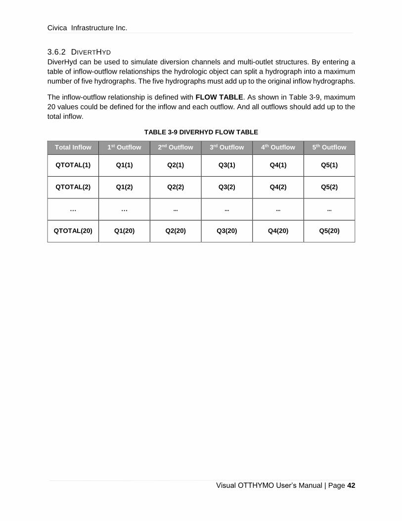
3.6.2 DIVERTHYD
DiverHyd can be used to simulate diversion channels and multi-outlet structures. By entering a
table of inflow-outflow relationships the hydrologic object can split a hydrograph into a maximum
number of five hydrographs. The five hydrographs must add up to the original inflow hydrographs.
The inflow-outflow relationship is defined with FLOW TABLE. As shown in Table 3-9, maximum
20 values could be defined for the inflow and each outflow. And all outflows should add up to the
total inflow.
TABLE 3-9 DIVERHYD FLOW TABLE
Total Inflow 1st Outflow 2nd Outflow 3rd Outflow 4th Outflow 5th Outflow
QTOTAL(1) Q1(1) Q2(1) Q3(1) Q4(1) Q5(1)
QTOTAL(2) Q1(2) Q2(2) Q3(2) Q4(2) Q5(2)
… … … … … …
QTOTAL(20) Q1(20) Q2(20) Q3(20) Q4(20) Q5(20)

Civica Infrastructure Inc.
Visual OTTHYMO User’s Manual | Page 43
3.7 FLOW MERGING HYDROLOGIC OBJECTS
AddHyd is used to add any number of hydrographs. There is no parameter associated with
AddHyd.
3.8 OTHER HYDROLOGICAL OBJECTS
3.8.1 READHYD
ReadHyd is used to read a previously saved hydrograph from a file. The parameter FILEPN is
the file name of the save hydrograph. For file format, see 11.4.
3.8.2 STOREHYD
StoreHyd is used to enter ordinates of a hydrograph directly.
TABLE 3-10 STOREHYD PARAMETERS
Parameter
Name Description Default Value
AREA The watershed area from which the hydrograph was derived (ha or
acre) 30
HYD POINTS A list of hydrograph ordinates, entered at time steps equals to DT.
Up to 2000 values can be entered (m3/s or ft3/s) Empty

Civica Infrastructure Inc.
Visual OTTHYMO User’s Manual | Page 44
4 VISUAL OTTHYMO MAIN WINDOW
4.1 OVERVIEW
The interface has been designed to provide plenty of working space for the schematic and map
model while maintaining easy access to the hydrologic objects and their associated parameters.
The layout consists of various regions as explained in the text below. Most of the windows are
dockable windows which could be docked to selected location. In case a window is closed, it could
be re-opened through the Windows drop-down list in Home tab.
FIGURE 4-1 LAYOUT OF MAIN INTERFACE
The Toolbox gives the user access to all the hydrologic objects (e.g. Hydrographs, Routing Rou-
tines) for the respective project type. Each object is categorized for ease of access, and repre-
sented by an icon in the Toolbox.
The Toolbar provides easy access to common program features found in all Windows programs
(e.g. New, Open, Save, etc) as well as the VO’s own program features (e.g. Climate Library,
Hydrograph, etc.). Here, there can be up to three ribbon tabs (Home, GIS and Simulation).
The Project Manager shows the user the names of all the hydrologic scenarios within the open
project. This window also provides a simple way of modifying those scenarios (e.g. Add, Delete).
It also holds the climate data used in the simulation.
The Properties window provides the user with the main form for inputting hydrologic object pa-
rameters (e.g. catchment area, slope, length). This window is where the bulk of the data entry
takes place.
Toolbox
Toolbar
Project Manager
Schematic View
Map View
Properties
Parameter Tables / Hydrograph Results / Error List

Civica Infrastructure Inc.
Visual OTTHYMO User’s Manual | Page 45
The Schematic View is where the user builds their model schematic from the hydrologic objects
in the Toolbox. Objects are dragged from the Toolbox and dropped on the Designer Canvas.
Links are generated by dragging the centre of a glyph to the centre of another. For more infor-
mation, please refer to Chapter 6.
The Map View is the geospatial representation of the same model. Each hydrological object is
assigned to a geometry either from manual drawing or from existing GIS data. Hydrological ob-
jects of different type are in different layers. For more information, please refer to Chapter 7.
The Parameter Tables lists all parameter values in tables. It provides a spreadsheet-like envi-
ronment for data editing.
The simulation results are summarized in Hydrograph Results / Water Balance Results. For
single-event simulation, it has peak flow and runoff volume. For continuous simulation, average
annual water balance components are summarized.
The model is checked against established rules. Violations are categorized to warnings and er-
rors, which will be shows in Error List window. Models with errors can’t run a simulation.
4.2 TOOLBOX
The following tables list the hydrologic objects from the Toolbox and their name. Hydrologic ob-
jects with bold font could be used in both single-event and continuous simulation. Users of previ-
ous versions of Visual OTTHYMO and OTTHYMO will recognize these commands. For a more
detailed description of each command, refer to Chapter 3.
TABLE 4-1 OTTHYMO COMMANDS
Generate Hydrograph Objects
STANDHYD SCSHYD
NASHYD WILHYD
Route Hydrograph Objects
ROUTE CHANNEL ROUTE MUSK-CUNGE
ROUTE PIPE ROUTE RESERVOIR
Flow Manipulation Hydrograph Objects
ADDHYD SHIFT HYD

Civica Infrastructure Inc.
Visual OTTHYMO User’s Manual | Page 46
DIVERT HYD DUHYD
Manual Input Hydrograph Objects
READ HYD STORE HYD
4.3 TOOLBAR
The following tables lists the icons from the Toolbar and their name. There are three (3) tabs in
total: Home, GIS and Simulation. A brief description of the contents of these tabs are given in to
Table 4-3 Table 4-5. For a more detailed description of each Toolbar item, please refer to the
Help System within the program.
TABLE 4-2 FILE MENU
Icon Command Icon Command
New Project
Creates a new project
Open Project
Opens an existing project
Save Project
Saves the current project
Save Project As
Saves the current project under a
different name
Import
Import scenarios
Export
Export the current scenario
Copy to Clipboard
Copy select objects to clipboard
Print the canvas

Civica Infrastructure Inc.
Visual OTTHYMO User’s Manual | Page 47
TABLE 4-3 HOME TAB
Icon Command Icon Command
New Project
Creates a new project
Delete
Deletes selection
Open Project
Opens an existing project
Undo
Removes the latest action
Save Project
Saves the current project
Redo
Repeats the last action
Save Project As
Saves the current project under
a different name
Edit History
Displays list of actions performed
by the modeler(s)
Copy
Copies the selection to the clip-
board
Find
Locates a specific object by ID or
name
Cut
Extracts the selection to the clip-
board
Windows
Provides dropdown for selection of
windows to be displayed
Paste
Pastes copied or cut hydrologic
objects
Options
Accesses window to define gen-
eral settings details such as Unit
and Precision, etc.
Civica Infrastructure Inc.
Visual OTTHYMO User’s Manual | Page 48
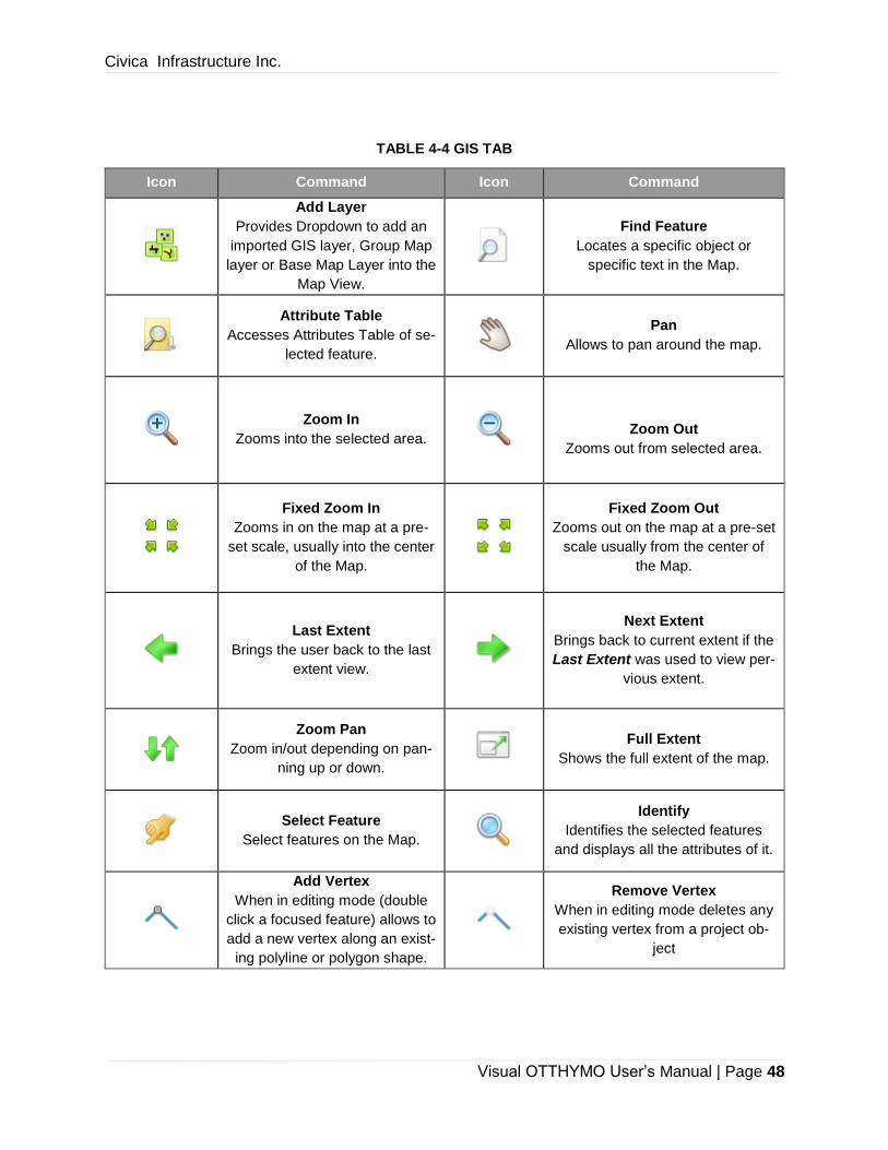
TABLE 4-4 GIS TAB
Icon Command Icon Command
Add Layer
Provides Dropdown to add an
imported GIS layer, Group Map
layer or Base Map Layer into the
Map View.
Find Feature
Locates a specific object or
specific text in the Map.
Attribute Table
Accesses Attributes Table of se-
lected feature.
Pan
Allows to pan around the map.
Zoom In
Zooms into the selected area.
Zoom Out
Zooms out from selected area.
Fixed Zoom In
Zooms in on the map at a pre-
set scale, usually into the center
of the Map.
Fixed Zoom Out
Zooms out on the map at a pre-set
scale usually from the center of
the Map.
Last Extent
Brings the user back to the last
extent view.
Next Extent
Brings back to current extent if the
Last Extent was used to view per-
vious extent.
Zoom Pan
Zoom in/out depending on pan-
ning up or down.
Full Extent
Shows the full extent of the map.
Select Feature
Select features on the Map.
Identify
Identifies the selected features
and displays all the attributes of it.
Add Vertex
When in editing mode (double
click a focused feature) allows to
add a new vertex along an exist-
ing polyline or polygon shape.
Remove Vertex
When in editing mode deletes any
existing vertex from a project ob-
ject

Civica Infrastructure Inc.
Visual OTTHYMO User’s Manual | Page 49
Icon Command Icon Command
Edit Tool
Select features on map to edit
Add Link
Create the link between two hydro-
logic objects on map
Point
Allows to snap to a point.
MidPoint
Allows to snap to a vertex when
required
Vertex
Allows to snap to the vertex.
Intersection
Allows to snap to the intersection
Edge
Allows to snap along the edge of
polyline or polygon.
EndPoint
Allows to snap to the end point of
polyline or polygon.
Assign Geometry
Assign geometry to hydrologic
objects
Calculate CN
Calculate CN based on soil and
landuse layer and assign to
NasHyd or StandHyd
Calculate Area Weighted
Calculate the parameter values
with given layer using area-
weighted method
Civica Infrastructure Inc.
Visual OTTHYMO User’s Manual | Page 50
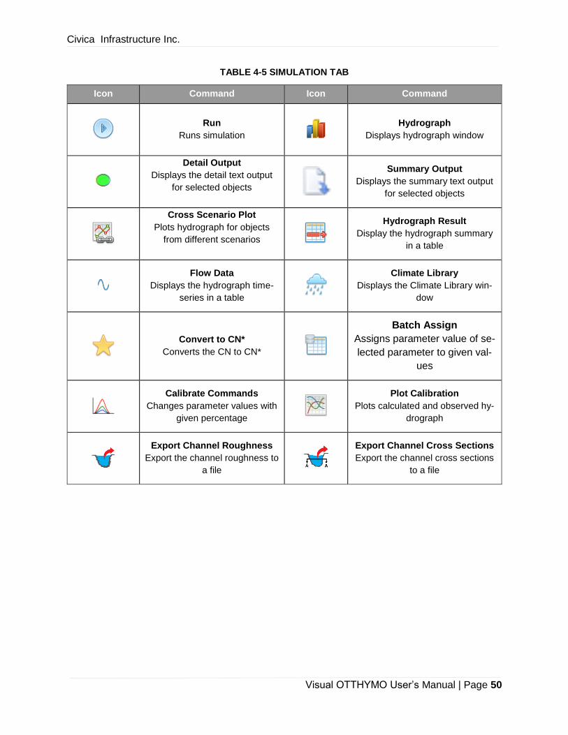
TABLE 4-5 SIMULATION TAB
Icon Command Icon Command
Run
Runs simulation
Hydrograph
Displays hydrograph window
Detail Output
Displays the detail text output
for selected objects
Summary Output
Displays the summary text output
for selected objects
Cross Scenario Plot
Plots hydrograph for objects
from different scenarios
Hydrograph Result
Display the hydrograph summary
in a table
Flow Data
Displays the hydrograph time-
series in a table
Climate Library
Displays the Climate Library win-
dow
Convert to CN*
Converts the CN to CN*
Batch Assign
Assigns parameter value of se-
lected parameter to given val-
ues
Calibrate Commands
Changes parameter values with
given percentage
Plot Calibration
Plots calculated and observed hy-
drograph
Export Channel Roughness
Export the channel roughness to
a file
Export Channel Cross Sections
Export the channel cross sections
to a file

Civica Infrastructure Inc.
Visual OTTHYMO User’s Manual | Page 51
4.4 PROJECT MANAGER
The Project Manager is to manage the scenarios and climate data in the project. By default, it’s
located on the right-hand side besides the Properties window.
The Project Manager in Continuous OTTHYMO project has two more sections (Temperature
Data and Evaporation Data) than the one in Single-event OTTHYMO project as shown in Figure
4-2. The two more sections enable to have long-term temperature and evaporation data for the
model simulation.
FIGURE 4-2 PROJEC MANAGER
On the top of Project Manager is the tool bar. The buttons are described in Table 4-6.
TABLE 4-6 PROJECT MANAGER TOOLBAR
Icon Command Icon Command
Add
Add Scenario or Open Climate
Library
Duplicate
Duplicate Selected Item
Delete
Delete Selected Item
Climate Library
Open Climate Library
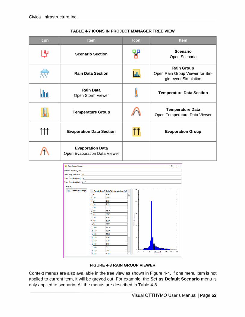
Below the toolbar is a tree view of scenarios and climate data. Items are represented with icons
described in Table 4-7. Some of the sections would open the detail information window by double-
click, which is also described in Table 4-7. For example, the Rain Group Viewer (Figure 4-3) will
be opened by double-clicking on Rain Group section.
Single-event Continuous
Civica Infrastructure Inc.
Visual OTTHYMO User’s Manual | Page 52
TABLE 4-7 ICONS IN PROJECT MANAGER TREE VIEW
Icon Item Icon Item
Scenario Section
Scenario
Open Scenario
Rain Data Section
Rain Group
Open Rain Group Viewer for Sin-
gle-event Simulation
Rain Data
Open Storm Viewer Temperature Data Section
Temperature Group
Temperature Data
Open Temperature Data Viewer
Evaporation Data Section
Evaporation Group
Evaporation Data
Open Evaporation Data Viewer
FIGURE 4-3 RAIN GROUP VIEWER
Context menus are also available in the tree view as shown in Figure 4-4. If one menu item is not
applied to current item, it will be greyed out. For example, the Set as Default Scenario menu is
only applied to scenario. All the menus are described in Table 4-8.

Civica Infrastructure Inc.
Visual OTTHYMO User’s Manual | Page 53
FIGURE 4-4 PROJECT MANAGER CONTEXT MENU
TABLE 4-8 CONTEXT MENU IN PROJECT MANAGER TREE VIEW
Menu Command Applicable Items
Set as Default Scenario Set selected scenario as default scenario
Add… Add Scenario or Open Climate Library
Edit… Open Scenario or Data Viewer
Rename Rename the selected item
Delete Delete Selected Item
Duplicate Duplicate Selected Item
4.5 PROPERTIES
Properties window (Figure 4-5) shows all properties of selected hydrologic object(s) or current
scenario. To use Properties window:
▪ Select single hydrologic object in Map View or Schematic View to view and edit all prop-
erties of the object;
▪ Select multiple hydrologic objects in Map View or Schematic View to view and edit com-
mon properties;
▪ Deselect all hydrologic objects to view and edit scenario properties.
Civica Infrastructure Inc.
Visual OTTHYMO User’s Manual | Page 54
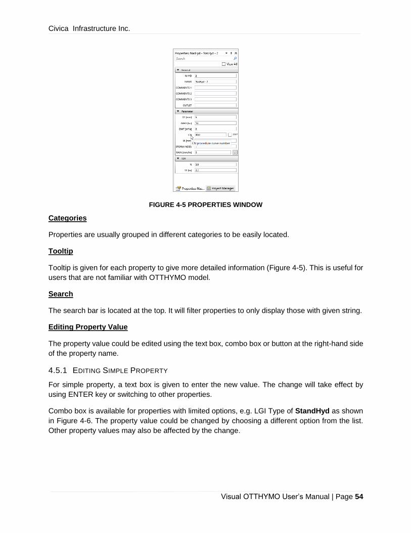
FIGURE 4-5 PROPERTIES WINDOW
Categories
Properties are usually grouped in different categories to be easily located.
Tooltip
Tooltip is given for each property to give more detailed information (Figure 4-5). This is useful for
users that are not familiar with OTTHYMO model.
Search
The search bar is located at the top. It will filter properties to only display those with given string.
Editing Property Value
The property value could be edited using the text box, combo box or button at the right-hand side
of the property name.
4.5.1 EDITING SIMPLE PROPERTY
For simple property, a text box is given to enter the new value. The change will take effect by
using ENTER key or switching to other properties.
Combo box is available for properties with limited options, e.g. LGI Type of StandHyd as shown
in Figure 4-6. The property value could be changed by choosing a different option from the list.
Other property values may also be affected by the change.
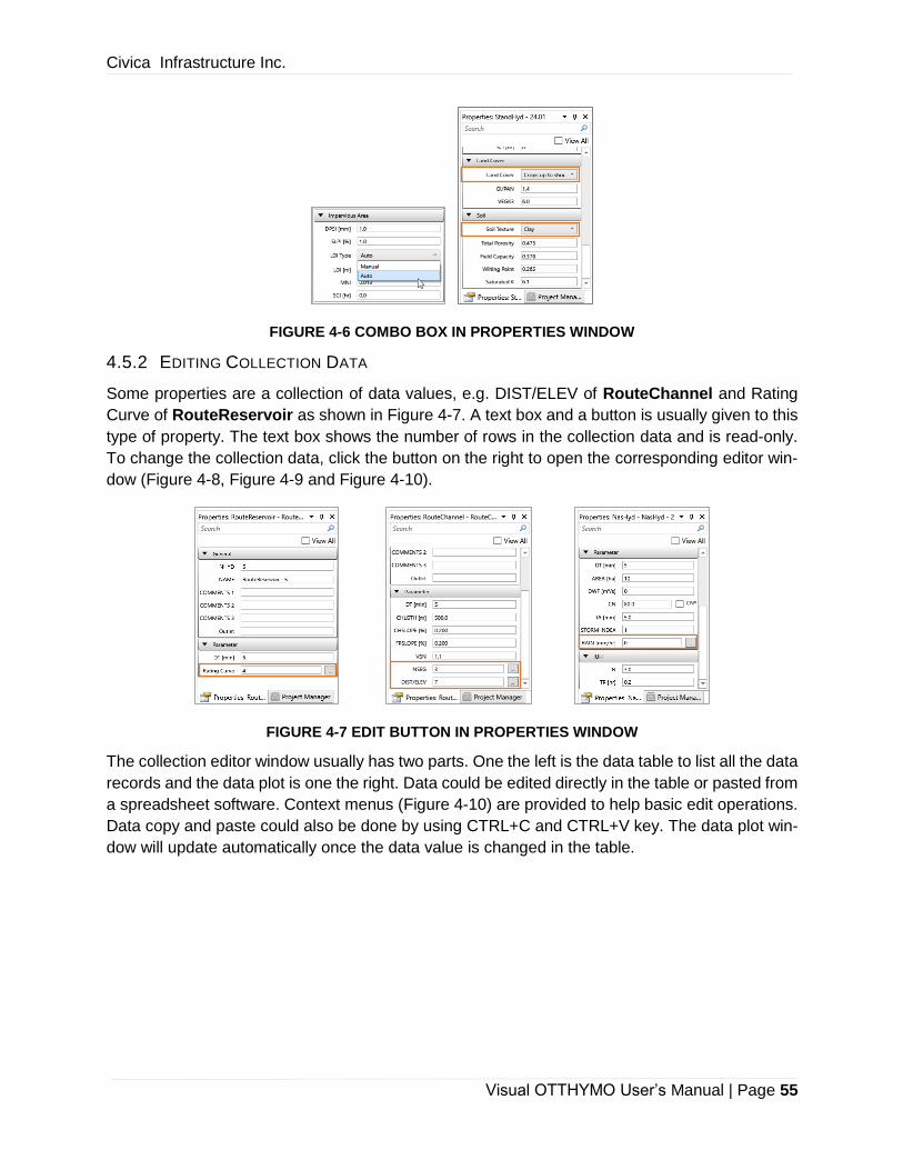
Civica Infrastructure Inc.
Visual OTTHYMO User’s Manual | Page 55
FIGURE 4-6 COMBO BOX IN PROPERTIES WINDOW
4.5.2 EDITING COLLECTION DATA
Some properties are a collection of data values, e.g. DIST/ELEV of RouteChannel and Rating
Curve of RouteReservoir as shown in Figure 4-7. A text box and a button is usually given to this
type of property. The text box shows the number of rows in the collection data and is read-only.
To change the collection data, click the button on the right to open the corresponding editor win-
dow (Figure 4-8, Figure 4-9 and Figure 4-10).
FIGURE 4-7 EDIT BUTTON IN PROPERTIES WINDOW
The collection editor window usually has two parts. One the left is the data table to list all the data
records and the data plot is one the right. Data could be edited directly in the table or pasted from
a spreadsheet software. Context menus (Figure 4-10) are provided to help basic edit operations.
Data copy and paste could also be done by using CTRL+C and CTRL+V key. The data plot win-
dow will update automatically once the data value is changed in the table.

Civica Infrastructure Inc.
Visual OTTHYMO User’s Manual | Page 56
FIGURE 4-8 CHANNEL ROUGHNESS SEGMENT AND RAINFALL EDITOR
FIGURE 4-9 CHANNEL DISTANCE ELEVATION EDITOR
FIGURE 4-10 RESERVOIR DISCHARGE STORAGE RATING CURVE EDITOR
4.5.3 EDITING LOSS ROUTINE OF STANDHYD
The LOSS property of StandHyd is to change the loss routine for pervious area. As different
parameters are used in these routines, it needs to be edited in a separate editor. To open this
editor, the LOSS property is similar with the one for collection data to have a text box and a button.
To edit the loss routine, click on the button to open the LOSS Editor where the loss routine type
and corresponding parameters could be changed.

Civica Infrastructure Inc.
Visual OTTHYMO User’s Manual | Page 57
FIGURE 4-11 LOSS PROPERTY AND LOSS EDITOR
4.5.4 CN* FLAG
When SCS equation is used to calculate the rainfall excess in pervious area, the Curve Number
(CN) is the most important parameter. From the early research of OTTHYMO, it has been recom-
mended to use the modified CN, i.e. CN*. VO has provided a tool (Convert to CN*) to convert
the CNII to CN*. To indicate the conversion has been conducted, a check box is given on the right
of the CN property as shown in Figure 4-12. The sole purpose of this check box is to tell the CNII
has been converted to CN* to avoid repeating the conversion. It’s not recommended to manually
uncheck or check it although it doesn’t affect the CN value.
FIGURE 4-12 CN* CHECK BOX IN PROPERTIES WINDOW
4.6 PARAMETER TABLES
Parameter Tables window provides a spreadsheet environment for parameter editing. By default,
it’s located at the bottom of the main interface.
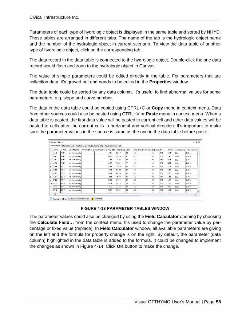
Civica Infrastructure Inc.
Visual OTTHYMO User’s Manual | Page 58
Parameters of each type of hydrologic object is displayed in the same table and sorted by NHYD.
These tables are arranged in different tabs. The name of the tab is the hydrologic object name
and the number of the hydrologic object in current scenario. To view the data table of another
type of hydrologic object, click on the corresponding tab.
The data record in the data table is connected to the hydrologic object. Double-click the one data
record would flash and zoon to the hydrologic object in Canvas.
The value of simple parameters could be edited directly in the table. For parameters that are
collection data, it’s greyed out and needs to be edited in the Properties window.
The data table could be sorted by any data column. It’s useful to find abnormal values for some
parameters, e.g. slope and curve number.
The data in the data table could be copied using CTRL+C or Copy menu in context menu. Data
from other sources could also be pasted using CTRL+V or Paste menu in context menu. When a
data table is pasted, the first data value will be pasted to current cell and other data values will be
pasted to cells after the current cells in horizontal and vertical direction. It’s important to make
sure the parameter values in the source is same as the one in the data table before paste.
FIGURE 4-13 PARAMETER TABLES WINDOW
The parameter values could also be changed by using the Field Calculator opening by choosing
the Calculate Field… from the context menu. It’s used to change the parameter value by per-
centage or fixed value (replace). In Field Calculator window, all available parameters are giving
on the left and the formula for property change is on the right. By default, the parameter (data
column) highlighted in the data table is added to the formula. It could be changed to implement
the changes as shown in Figure 4-14. Click OK button to make the change.

Civica Infrastructure Inc.
Visual OTTHYMO User’s Manual | Page 59
FIGURE 4-14 FIELD CALCULATOR WINDOW
4.7 HYDROGRAPH RESULTS / WATER BALANCE RESULTS
The Hydrograph Results and Water Balance Results window is the same window appearing
differently for single-event simulation and continuous simulation. By default, this window is at the
bottom of the main interface. It’s used to show the summary results of each hydrologic object.
FIGURE 4-15 HYDROGRAPH RESULTS WINDOW FOR SINGLE-EVENT SIMULATION
FIGURE 4-16 WATER BALANCE RESULTS WINDOW FOR CONTINUOUS SIMULATION
For single-event simulation, the summary is the peak flow and runoff volume of the hydrograph.
For continuous simulation, it’s the peak flow and average annual amount of each water balance
component. The summaries are shown in a data table for each available hydrological object. Data
could be sorted by any column.
In case there are multiple simulation runs, only summary results of select run (selected in scenario
property) is shown in the table. To switch to another run, select the run from the drop-down list

Civica Infrastructure Inc.
Visual OTTHYMO User’s Manual | Page 60
above the data table. It’s possible to show summary results of all runs by click the Show All Runs
button.
Same as Parameter Tables window, the hydrologic object could be zoomed to by double-clicking
on the data record.
4.8 ERROR LIST
The Error List window shows the errors and warnings in the model. By default, it’s located at the
bottom of the main interface.
Certain rules apply to an OTTHYMO model. If these rules are not met, a warning or an error will
show in the Error List window. A model with error can’t run. The error and warning information is
shown in a data table with the error type, hydrologic object ID and name, hydrologic object type
and error message. An error will be shown as and a warning will be . Same as Parameter
Tables window and Hydrograph Results window, the hydrologic object could be zoomed to by
double-clicking on the data record in the table. Note that, a read outline is added to the object
icon if an error is found. For example, a RouteChannel without source link will be shown as
in canvas.
FIGURE 4-17 ERROR LIST WINDOW
The data table could be filtered to only show errors or warnings. The three buttons on the top is
to switch each message on and off. By default, all errors and warning are shown in the table.
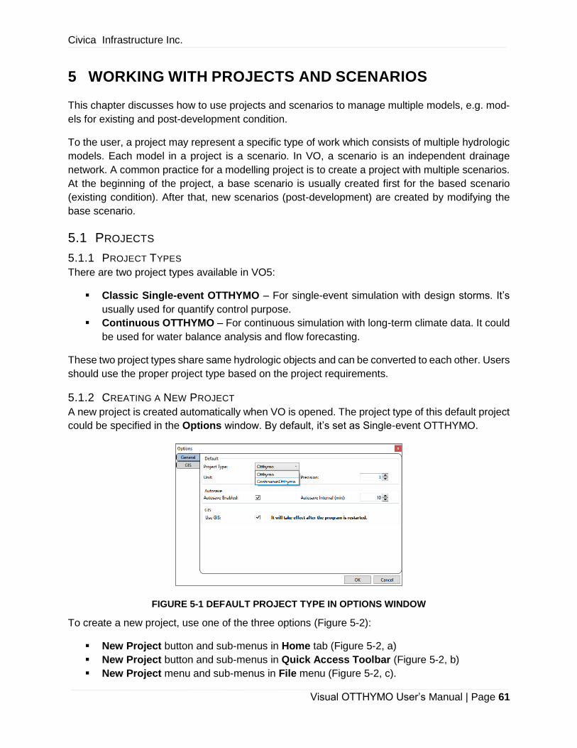
Civica Infrastructure Inc.
Visual OTTHYMO User’s Manual | Page 61
5 WORKING WITH PROJECTS AND SCENARIOS
This chapter discusses how to use projects and scenarios to manage multiple models, e.g. mod-
els for existing and post-development condition.
To the user, a project may represent a specific type of work which consists of multiple hydrologic
models. Each model in a project is a scenario. In VO, a scenario is an independent drainage
network. A common practice for a modelling project is to create a project with multiple scenarios.
At the beginning of the project, a base scenario is usually created first for the based scenario
(existing condition). After that, new scenarios (post-development) are created by modifying the
base scenario.
5.1 PROJECTS
5.1.1 PROJECT TYPES
There are two project types available in VO5:
▪ Classic Single-event OTTHYMO – For single-event simulation with design storms. It’s
usually used for quantify control purpose.
▪ Continuous OTTHYMO – For continuous simulation with long-term climate data. It could
be used for water balance analysis and flow forecasting.
These two project types share same hydrologic objects and can be converted to each other. Users
should use the proper project type based on the project requirements.
5.1.2 CREATING A NEW PROJECT
A new project is created automatically when VO is opened. The project type of this default project
could be specified in the Options window. By default, it’s set as Single-event OTTHYMO.
FIGURE 5-1 DEFAULT PROJECT TYPE IN OPTIONS WINDOW
To create a new project, use one of the three options (Figure 5-2):
▪ New Project button and sub-menus in Home tab (Figure 5-2, a)
▪ New Project button and sub-menus in Quick Access Toolbar (Figure 5-2, b)
▪ New Project menu and sub-menus in File menu (Figure 5-2, c).

Civica Infrastructure Inc.
Visual OTTHYMO User’s Manual | Page 62
FIGURE 5-2 THREE OPTIONS TO CREATE A NEW PROJECT
Similar options are also available for Open Project, Save Project and Save Project As.
5.1.3 OPENING AN EXISTING PROJECT
To open an existing project, click the Open Project button or menu in Home tab, Quick
Access Toolbar or File Menu. The Open window will appear to browse VO project files (*.voprj).
VO maintains a recent project file list. When a project is opened at the first time, it will be added
to the list. To open it again, simply select it from the Recent Files list in File Menu.
FIGURE 5-3 RECENT PROJECT FILE LIST
A project file could also be opened by double-clicking on the project file in File Explorer. The
project file (*.voprj) has been registered with VO and appears with icon in File Explorer.
5.1.4 SAVING A PROJECT
All changes made to a project is temporary until they are saved. To save changes to the project
file, click the Save Project button or menu in Home tab, Quick Access Toolbar or File Menu.
The working project could also be saved to another location with the Save Project As button
or menu in Home tab, Quick Access Toolbar or File Menu.
Note that the imported layers are not saved in the project file. You should make sure the file
sources are valid.
5.2 SCENARIOS
In VO, a scenario is an independent drainage network. It includes all hydrological objects and the
links between them. It could be displayed in Map View and Schematic View. All scenarios are
list in Project Manager.
(a) (b) (c)

Civica Infrastructure Inc.
Visual OTTHYMO User’s Manual | Page 63
FIGURE 5-4 SCENAIOS IN PROJECT MANAGER
5.2.1 CREATING A NEW SCENARIO
To create an empty scenario, click the Add button at the top of the Project Manager or select
Add menu from the context menu. The Scenario Create window will appear (Figure 5-5). Enter
the name and description and click OK button to create the scenario. The new scenario will be
opened immediately in Schematic View and/or Map View.
FIGURE 5-5 SCENARIO CREATE WINDOW
5.2.2 DUPLICATING AN EXISTING SCENARIO
In often cases, a new scenario is created by copying an existing scenario and then make changes.
To do this:
1. Select an existing scenario in Project Manager and then click the Duplicate button at
the top of the Project Manager or select Duplicate menu from the context menu.
2. The Duplicate Scenario window will appear (Figure 5-6)
3. Enter the name of the new scenario.
4. Options are available to duplicate both Commands and Runs. Always keep the Com-
mands checked. If different climate data will be used in the new scenario, uncheck the
Runs.
5. Click the Duplicate button at the bottom to create the new scenario.
FIGURE 5-6 DUPLICATE SCENARIO WINDOW
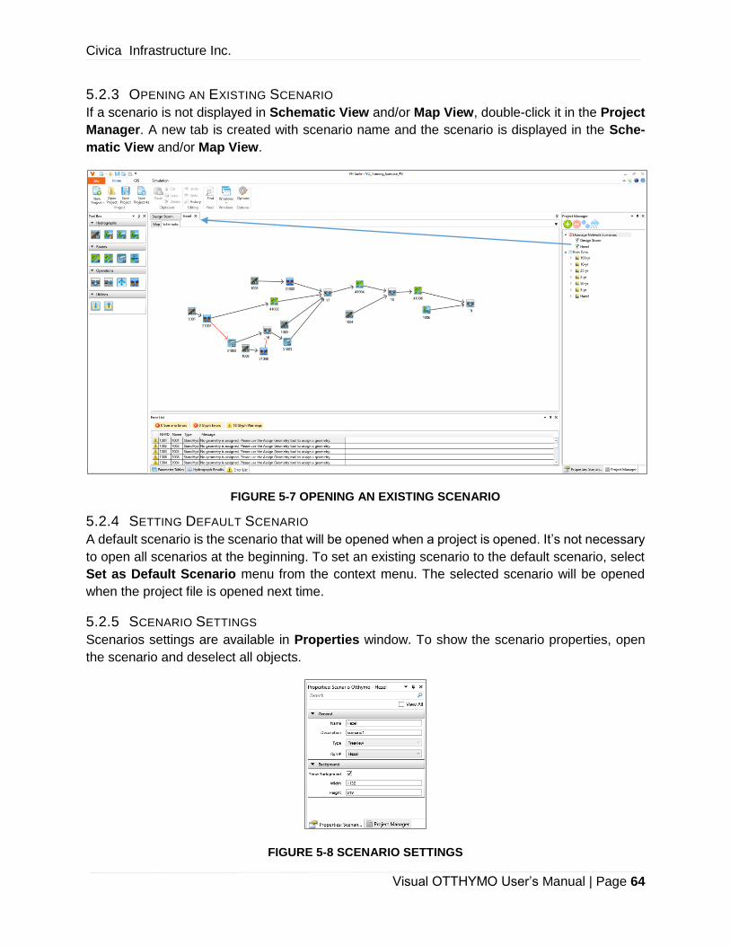
Civica Infrastructure Inc.
Visual OTTHYMO User’s Manual | Page 64
5.2.3 OPENING AN EXISTING SCENARIO
If a scenario is not displayed in Schematic View and/or Map View, double-click it in the Project
Manager. A new tab is created with scenario name and the scenario is displayed in the Sche-
matic View and/or Map View.
FIGURE 5-7 OPENING AN EXISTING SCENARIO
5.2.4 SETTING DEFAULT SCENARIO
A default scenario is the scenario that will be opened when a project is opened. It’s not necessary
to open all scenarios at the beginning. To set an existing scenario to the default scenario, select
Set as Default Scenario menu from the context menu. The selected scenario will be opened
when the project file is opened next time.
5.2.5 SCENARIO SETTINGS
Scenarios settings are available in Properties window. To show the scenario properties, open
the scenario and deselect all objects.
FIGURE 5-8 SCENARIO SETTINGS
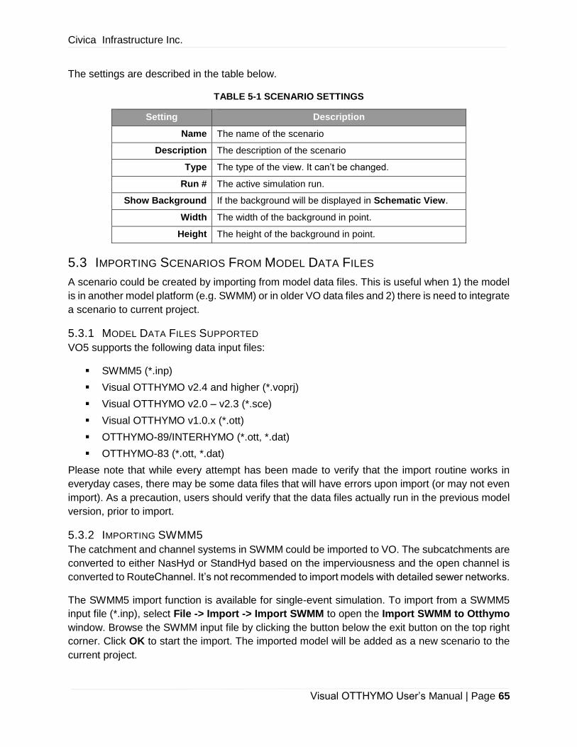
Civica Infrastructure Inc.
Visual OTTHYMO User’s Manual | Page 65
The settings are described in the table below.
TABLE 5-1 SCENARIO SETTINGS
Setting Description
Name The name of the scenario
Description The description of the scenario
Type The type of the view. It can’t be changed.
Run # The active simulation run.
Show Background If the background will be displayed in Schematic View.
Width The width of the background in point.
Height The height of the background in point.
5.3 IMPORTING SCENARIOS FROM MODEL DATA FILES
A scenario could be created by importing from model data files. This is useful when 1) the model
is in another model platform (e.g. SWMM) or in older VO data files and 2) there is need to integrate
a scenario to current project.
5.3.1 MODEL DATA FILES SUPPORTED
VO5 supports the following data input files:
▪ SWMM5 (*.inp)
▪ Visual OTTHYMO v2.4 and higher (*.voprj)
▪ Visual OTTHYMO v2.0 – v2.3 (*.sce)
▪ Visual OTTHYMO v1.0.x (*.ott)
▪ OTTHYMO-89/INTERHYMO (*.ott, *.dat)
▪ OTTHYMO-83 (*.ott, *.dat)
Please note that while every attempt has been made to verify that the import routine works in
everyday cases, there may be some data files that will have errors upon import (or may not even
import). As a precaution, users should verify that the data files actually run in the previous model
version, prior to import.
5.3.2 IMPORTING SWMM5
The catchment and channel systems in SWMM could be imported to VO. The subcatchments are
converted to either NasHyd or StandHyd based on the imperviousness and the open channel is
converted to RouteChannel. It’s not recommended to import models with detailed sewer networks.
The SWMM5 import function is available for single-event simulation. To import from a SWMM5
input file (*.inp), select File -> Import -> Import SWMM to open the Import SWMM to Otthymo
window. Browse the SWMM input file by clicking the button below the exit button on the top right
corner. Click OK to start the import. The imported model will be added as a new scenario to the
current project.

Civica Infrastructure Inc.
Visual OTTHYMO User’s Manual | Page 66
FIGURE 5-9 IMPORT SWMM TO OTTHYMO MODEL
5.3.3 IMPORTING VISUAL OTTHYMO V2.4 AND LATER
Importing a Visual OTTHYMO v2.4 and higher project file (*.voprj) is necessary when you want
to bring an existing scenario into your current project. This may be necessary if you are combining
projects or if you want to use an existing model scenario to build a new model.
Once you have your project open, select File -> Import -> Import VH Scenario (Current Project)
menu to browse the VO project file and open the Import Scenarios window as follows. All sce-
nario in the project is list in the window. You may want to only select the scenarios that you want
to import. Click Import Selected button at the bottom and the selected scenarios are added to
current project.
Before running your new scenario, you should check that the storm files and any external files
(e.g. READ HYD) are referenced to the proper location on your system.
FIGURE 5-10 IMPORT SCENARIO WINDOW
5.3.4 IMPORTING VISUAL OTTHYMO V2.0 - V2.3 DATA FILES
Scenarios in Visual OTTHYMO v2.0 – v2.3 are saved in separated files (*.sce). They could be
imported to current project with menu File -> Import -> Import VO2 Scenario (Current Project).
The scenario will be added to current project immediately after the import. Rain data will also be
imported.

Civica Infrastructure Inc.
Visual OTTHYMO User’s Manual | Page 67
FIGURE 5-11 IMPORTING VO2 SCENARIO FILE
5.3.5 IMPORTING CLASSIC OTTHYMO DATA FILES
The model file used in Visual OTTHYMO v1.0.x, OTTHYMO-89/INTERHYMO and OTTHYMO-
83 is in similar text file format. It may have the extension of ott, dat or txt. These files could be
imported as a new scenario to current project with menu File -> Import -> Import Scenario (Ot-
thymo 89). As the location of the hydrologic objects are not specified in the model file, the objects
will be arranged from top to bottom. The most upstream objects will be located on the top. Their
locations could be changed later to represent the shape of the drainage network.
Any commands that are not included in VO5 are ignored during the import. These commands
may include COMPUTE VOLUME, PRINT HYD, PLOT HYD, SAVE HYD and ERROR ANALY-
SIS.

Civica Infrastructure Inc.
Visual OTTHYMO User’s Manual | Page 68
FIGURE 5-12 IMPORTING CLASSIC OTTHYMO MODEL FILE

Civica Infrastructure Inc.
Visual OTTHYMO User’s Manual | Page 69
6 WORKING WITH CANVAS
Canvas is where the hydrologic objects could be visually created and connected with icons. Ini-
tially introduced in version 1, it has transformed the way to create a OTTHYMO model, from text
file editing to LEGO-like structure building. The time spent on model creation has been signifi-
cantly reduced. And the need to remember format of various commands has been removed.
Building a model with VO is enjoyable.
6.1 ADDING BACKGROUND
A background showing the study area helps the modelers to place the hydrologic objects and the
reviewers to quickly understand the model structure.
To add the background:
1. Select the Background -> Change Background… menu from the Canvas context menu.
2. Select the background picture file in the Select an Image window. It supports JPEG, PNG
and BMP format.
3. Click Open button to add the selected picture file as the Canvas background.
4. Use the navigation functions to Pan, Zoom In or Zoom Out the Canvas until the back-
ground is in desired location.
5. Change the width and height of the background in the scenario properties window if nec-
essary. Note that the aspect ratio is not locked.
FIGURE 6-1 ADDING BACKGROUND
To remove background, select the Background -> Remove Background menu in Canvas con-
text menu.

Civica Infrastructure Inc.
Visual OTTHYMO User’s Manual | Page 70
To hide background, uncheck the Show Background in the scenario properties window. Note
that this is different from removing background. The background is still in the scenario.
6.2 ADDING HYDROLOGIC OBJECTS
Hydrologic objects are added to the Canvas by dragging the hydrologic objects icons from the
Toolbox and then dropping on the canvas.
FIGURE 6-2 ADDING HYDROGLOC OBJECTS ON CANVAS
New hydrologic objects could also be created by copying existing objects. To do this:
1. Select the objects to be copied. Multiple objects could be copied at the same time.
2. Copy the selected objects with either of the three options:
a. Copy button in Home Tab
b. Copy menu in the context menu
c. CTRL + C keys.
3. Similarly, paste the copied objects with one of the three options:
a. Paste button in Home Table
b. Paste menu in the context menu
c. CTRL + V keys.

Civica Infrastructure Inc.
Visual OTTHYMO User’s Manual | Page 71
FIGURE 6-3 COPYING AND PASTING HYDROLOGIC OBJECT ON CANVAS
6.3 SELECTING HYDROLOGIC OBJECTS
An individual hydrologic object is selected by moving the mouse curse on top of the object icon
and press the left button. A blue outline will be added to the object icon.
FIGURE 6-4 INDIVIDUAL OBJECT SELECTION ON CANVAS
Multiple objects are selected by holding the CTRL or SHIFT key and then selecting each object.

Civica Infrastructure Inc.
Visual OTTHYMO User’s Manual | Page 72
FIGURE 6-5 MULTIPLE OBJECTS SELECTION ON CANVAS
Adjacent objects could also be selected by dragging a rectangle covering all the objects. There is
no difference on how the rectangle is created (e.g. from left top corner to right bottom corner).
FIGURE 6-6 MUTIPLE OBJETS SELECTION WITH RECTANGLE
FIGURE 6-7 SELECTION FUNCTIONS IN CANVAS CONTEXT MENU
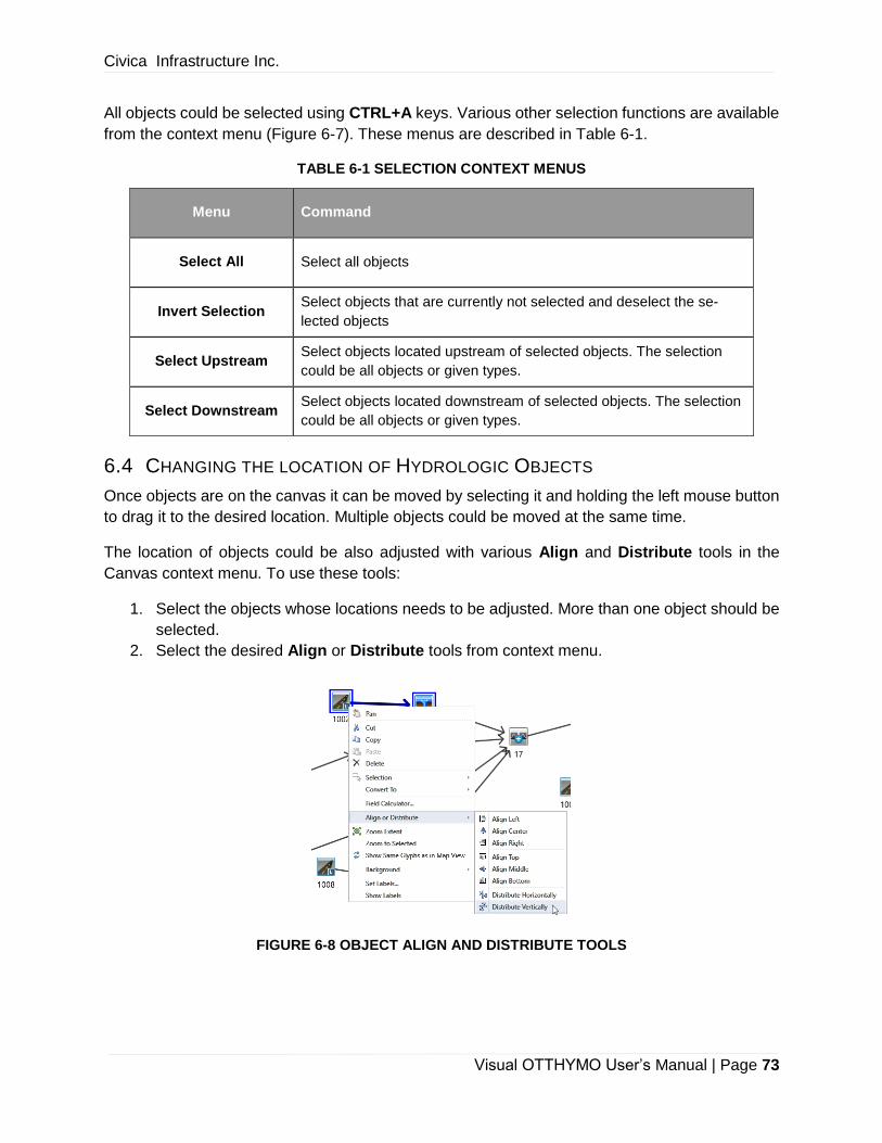
Civica Infrastructure Inc.
Visual OTTHYMO User’s Manual | Page 73
All objects could be selected using CTRL+A keys. Various other selection functions are available
from the context menu (Figure 6-7). These menus are described in Table 6-1.
TABLE 6-1 SELECTION CONTEXT MENUS
Menu Command
Select All Select all objects
Invert Selection Select objects that are currently not selected and deselect the se-
lected objects
Select Upstream Select objects located upstream of selected objects. The selection
could be all objects or given types.
Select Downstream Select objects located downstream of selected objects. The selection
could be all objects or given types.
6.4 CHANGING THE LOCATION OF HYDROLOGIC OBJECTS
Once objects are on the canvas it can be moved by selecting it and holding the left mouse button
to drag it to the desired location. Multiple objects could be moved at the same time.
The location of objects could be also adjusted with various Align and Distribute tools in the
Canvas context menu. To use these tools:
1. Select the objects whose locations needs to be adjusted. More than one object should be
selected.
2. Select the desired Align or Distribute tools from context menu.
FIGURE 6-8 OBJECT ALIGN AND DISTRIBUTE TOOLS

Civica Infrastructure Inc.
Visual OTTHYMO User’s Manual | Page 74
The available Align or Distribute tools are described in Table 6-2.
TABLE 6-2 OBJECT ALIGN AND DISTRIBUTE TOOLS
Icon Command Icon Command
Align Left
Align to the far left of all selected
objects
Align Top
Align to the top of all selected ob-
jects
Align Center
Align to the center (from far left
to far right) of all selected ob-
jects
Align Middle
Align to the middle (from top to
bottom) of all selected objects
Align Right
Align to the far right of all se-
lected objects
Align Bottom
Align to the bottom of all selected
objects
Distribute Horizontally
Distribute selected objects to
have same horizontal distance
Distribute Vertically
Distribute selected objects to have
same vertical distance
Note that the location change on canvas doesn’t has impact on its geospatial location in Map
View and vice versa.
6.5 LINKING HYDROLOGIC OBJECTS
The hydrologic objects and its immediate downstream objects are presented with an arrow point-
ing to the downstream objects. The arrow is called link in VO. To create a link on canvas:
1. Move the mouse cursor on top of the source object icon.
2. Keep left button pressed and move the mouse cursor on top of the downstream object
icon.
3. Release left button and the link will be created.
Some rules and guidelines for linking objects are given in Table 6-3. The link will not be added if
the number of input or output links reaches the limit.
Civica Infrastructure Inc.
Visual OTTHYMO User’s Manual | Page 75
TABLE 6-3 RULES FOR HYDROLOGIC OBJECT LINKS
Hydrologic Object # of Input Links # of Output Links Color
0 1 Black
1 1 Black
unlimited 1 Black
1 1 Black
1 5 Black
1 2
Minor: Red
Major: Black
0 1 Black
6.6 NAVIGATING CANVAS
The canvas could be easily navigated. Available navigation functions are described below.
1. Zoom In – Scroll the mouse wheel up.
2. Zoom Out – Scroll the mouse wheel down.
3. Pan – Move the canvas any direction. Available as the first context menu.
4. Zoom Extent – Zoom the canvas to show all object on the canvas (context menu).
5. Zoom to Selected – Zoom to selected objects (context menu).
6.7 CREATING LABELS
There are two type of labels on Canvas:
1. System label – The NHYD is label below each object icon which can’t be turned off.
2. Customized label – Certain properties and result summary could be labeled at the right
side of the object icon. The label content and content could be customized. It can also be
turned off.

Civica Infrastructure Inc.
Visual OTTHYMO User’s Manual | Page 76
FIGURE 6-9 TWO TYPES OF LABEL
To setup the customized label:
1. Select the objects you wish to create a label for.
2. Right-click and select the Set Labels from the context menu to open the Label Editor
window, which lists all available label items. Depending on the project and object type, the
available label items are different.
3. Drag and drop the label items from Available Properties list on the left to Selected Prop-
erties list on the right.
4. Change the label background color with the color picker at the bottom.
5. Click OK to create the label.
6. To show the labels on canvas, select Show Labels from the context menu.
Note that the result summary value is empty if the output is not available.
FIGURE 6-10 CREATING CUSTOMISED LABEL
Customized Label System Label

Civica Infrastructure Inc.
Visual OTTHYMO User’s Manual | Page 77
6.8 PRINTING MODEL SCHEMATIC
The mode schematic (including the background and labels) could be copied to clipboard or printed
directly. This is useful for project report.
To copy the schematic to clipboard, click the Copy to Clipboard button in File menu. Then it
could be pasted to a third-party software application. Note that only the selected objects will be
copied if the selection is not empty.
To print the mode schematic directly, click the Print button in File menu. The print preview
window will appear where it could be viewed and printed. The schematic was zoomed to have all
objects displayed and the selection doesn’t have impact.
FIGURE 6-11 PRINTE PREVIEW WINDOW

Civica Infrastructure Inc.
Visual OTTHYMO User’s Manual | Page 78
7 WORKING WITH THE MAP
Map is another way to create, parameterize and present an VO model. It adds geospatial location
information to each hydrological object and shows the model drainage network on the map. Sev-
eral benefits from using the map are:
1. Easier model creation with existing GIS data. For watershed and sub-watershed study,
various GIS data is usually available, which may include catchment, stream and output
layers. With Map View, the model drainage network could be created directly from these
layers without the need to create hydrologic objects one by one from scratch.
2. Reduced time for model parametrization. The geometry-based parameters (e.g. Area,
Length, etc.) are usually obtained from a third-party software and then entered in the
model. With geo-spatial location information, these parameters could be automatically cal-
culated. Tools are provided to calculate area weighted CN and Imperviousness.
3. Easier to understand. The model schematic may be difficult to understand without know-
ing the study area. This is improved with map by providing viewers the spatial context.
In VO, a scenario could be viewed in both the Schematic View (canvas) and the Map View
(Figure 7-1). By default, only one view is visible. To have them side-by-side (split view), drag Map
or Schematic tab to the desired location (Figure 7-2). Note that the Map View and GIS tab will
not be available if an ArcGIS license is not found.
FIGURE 7-1 DEFAULT LAYOUT OF MAP VIEW AND SCHEMATIC VIEW
Only Map View is visible

Civica Infrastructure Inc.
Visual OTTHYMO User’s Manual | Page 79
FIGURE 7-2 MAP VIEW AND SCHEMATIC VIEW SIDE-BY-SIDE
7.1 MAP VIEW LAYOUT
There are three components in the map view:
1. Table of Content – A tree view of all GIS layers. It controls the appearance of the layers.
2. Map – The main working space to display and edit hydrologic objects. The features could
be created, edited and selected.
3. Status Bar – Showing the coordinates.
FIGURE 7-3 MAP VIEW LAYOUT
Split View
Table of Content
Map
Status Bar
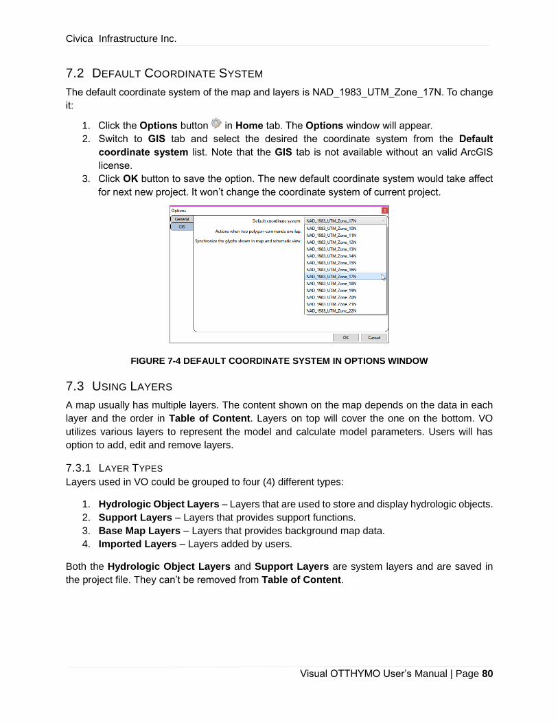
Civica Infrastructure Inc.
Visual OTTHYMO User’s Manual | Page 80
7.2 DEFAULT COORDINATE SYSTEM
The default coordinate system of the map and layers is NAD_1983_UTM_Zone_17N. To change
it:
1. Click the Options button in Home tab. The Options window will appear.
2. Switch to GIS tab and select the desired the coordinate system from the Default
coordinate system list. Note that the GIS tab is not available without an valid ArcGIS
license.
3. Click OK button to save the option. The new default coordinate system would take affect
for next new project. It won’t change the coordinate system of current project.
FIGURE 7-4 DEFAULT COORDINATE SYSTEM IN OPTIONS WINDOW
7.3 USING LAYERS
A map usually has multiple layers. The content shown on the map depends on the data in each
layer and the order in Table of Content. Layers on top will cover the one on the bottom. VO
utilizes various layers to represent the model and calculate model parameters. Users will has
option to add, edit and remove layers.
7.3.1 LAYER TYPES
Layers used in VO could be grouped to four (4) different types:
1. Hydrologic Object Layers – Layers that are used to store and display hydrologic objects.
2. Support Layers – Layers that provides support functions.
3. Base Map Layers – Layers that provides background map data.
4. Imported Layers – Layers added by users.
Both the Hydrologic Object Layers and Support Layers are system layers and are saved in
the project file. They can’t be removed from Table of Content.
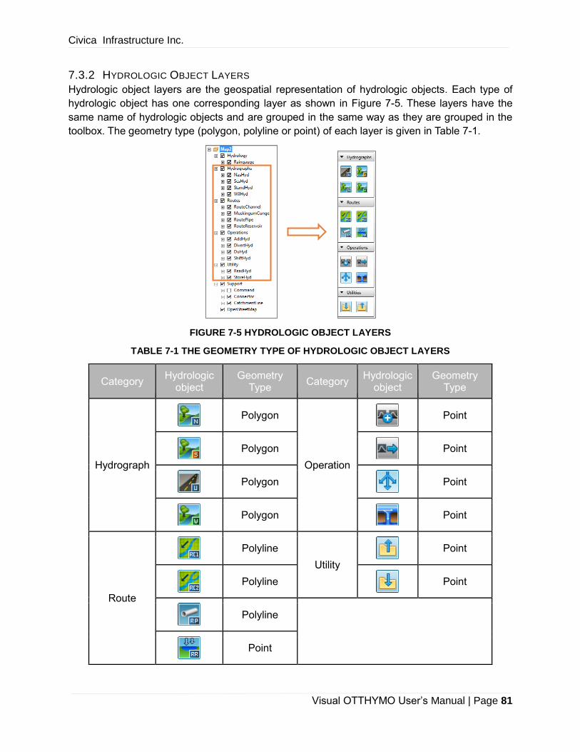
Civica Infrastructure Inc.
Visual OTTHYMO User’s Manual | Page 81
7.3.2 HYDROLOGIC OBJECT LAYERS
Hydrologic object layers are the geospatial representation of hydrologic objects. Each type of
hydrologic object has one corresponding layer as shown in Figure 7-5. These layers have the
same name of hydrologic objects and are grouped in the same way as they are grouped in the
toolbox. The geometry type (polygon, polyline or point) of each layer is given in Table 7-1.
FIGURE 7-5 HYDROLOGIC OBJECT LAYERS
TABLE 7-1 THE GEOMETRY TYPE OF HYDROLOGIC OBJECT LAYERS
Category Hydrologic
object Geometry
Type Category
Hydrologic object
Geometry Type
Hydrograph
Polygon
Operation
Point
Polygon
Point
Polygon
Point
Polygon
Point
Route
Polyline
Utility
Point
Polyline
Point
Polyline
Point
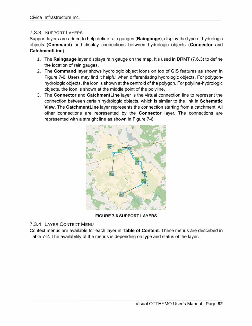
Civica Infrastructure Inc.
Visual OTTHYMO User’s Manual | Page 82
7.3.3 SUPPORT LAYERS
Support layers are added to help define rain gauges (Raingauge), display the type of hydrologic
objects (Command) and display connections between hydrologic objects (Connector and
CatchmentLine).
1. The Raingauge layer displays rain gauge on the map. It’s used in DRMT (7.6.3) to define
the location of rain gauges.
2. The Command layer shows hydrologic object icons on top of GIS features as shown in
Figure 7-6. Users may find it helpful when differentiating hydrologic objects. For polygon-
hydrologic objects, the icon is shown at the centroid of the polygon. For polyline-hydrologic
objects, the icon is shown at the middle point of the polyline.
3. The Connector and CatchmentLine layer is the virtual connection line to represent the
connection between certain hydrologic objects, which is similar to the link in Schematic
View. The CatchmentLine layer represents the connection starting from a catchment. All
other connections are represented by the Connector layer. The connections are
represented with a straight line as shown in Figure 7-6.
FIGURE 7-6 SUPPORT LAYERS
7.3.4 LAYER CONTEXT MENU
Context menus are available for each layer in Table of Content. These menus are described in
Table 7-2. The availability of the menus is depending on type and status of the layer.

Civica Infrastructure Inc.
Visual OTTHYMO User’s Manual | Page 83
TABLE 7-2 LAYER CONTEXT MENU
Menu Command
Attribute Table Open the attribute table of the layer
Remove Layer Remove the layer from map. Not available for hydrologic object layers and
support layers.
Move Layer Up Move the layer up one level
Move Layer Down Move the layer down one level
Layer Selectable Make the features selectable. Not available if it’s already selectable.
Layer Unselectable Make the feature un-selectable. Not available if it’s already un-selectable.
Zoom To Layer Change the map extent to show all features in the layer.
Deselect all but this Turn off all other layers but turn on current layer.
Select all but this Turn on all other layers but turn off current layer.
Show/Hide Arrows Show or hide arrows for polyline layer.
Export as Shape File Export current layer to shapefile
Export as CSV Export the attribute table to CSV file
File Source Display the file source.
Layer Properties Open the Layer Properties window.
7.3.5 ADDING A LAYER
To add a layer, using following button from Add Layer sub-menus in GIS tab:
▪ Feature Layer button to add any supported GIS data files.
▪ Group Layer button to add a new group layer.
▪ Basemap Layer button to add the base map layer.
The new layer will be added to the bottom of Table of Content. For feature layers, multiple layers
could be added at the same time.

Civica Infrastructure Inc.
Visual OTTHYMO User’s Manual | Page 84
7.3.6 MOVING LAYERS
The order of layers in Table of Content would affect how the features would show on map. Fea-
tures in top layers would cover features in bottom layers. It’s generally recommended to put point
and polyline layers on top of polygon layers to avoid any cover-up.
To move the layers in Table of Content, select the layer first and drag it to the new location.
Moving a group layer will also move all children layers.
FIGURE 7-7 MOVE LAYER IN TABLE OF CONTENT
Layers could all be moved by using the Move Layer Up and Move Layer Down context menu.
Layers in a group layer could only be moved inside that group.
7.3.7 REMOVING LAYERS
Base map layer and imported layers could be removed from Table of Content by selecting Re-
move Layer menu from the context menu. The hydrologic object layers and support layers can’t
be removed.
7.3.8 DEFINING LAYER VISIBILITY
The visibility of a layer could be defined using the check box in Table of Content and the Scale
Range setting in Layer Properties window.
Unchecking the check box would hide all features in that layer. For a group layer, it also hides
features belong to its children layers.
FIGURE 7-8 HIDE LAYER FEATURES
A scale range is the upper and lower scale limit when the features could be displayed on map.
It’s necessary to define the range when certain layer is not useful when the map is zoomed in or
out. To set up the scale range:
1. Select the Layer Properties menu from layer context menu. The Layer Properties win-
dow will appear.
2. Click on Scale Range tab. By default, the Show layer at all scales is checked, which
indicates that features in this layer would display at any scale.
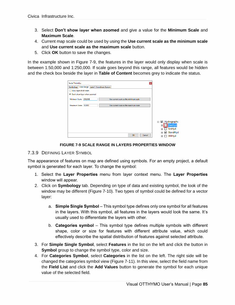
Civica Infrastructure Inc.
Visual OTTHYMO User’s Manual | Page 85
3. Select Don’t show layer when zoomed and give a value for the Minimum Scale and
Maximum Scale.
4. Current map scale could be used by using the Use current scale as the minimum scale
and Use current scale as the maximum scale button.
5. Click OK button to save the changes.
In the example shown in Figure 7-9, the features in the layer would only display when scale is
between 1:50,000 and 1:250,000. If scale goes beyond this range, all features would be hidden
and the check box beside the layer in Table of Content becomes grey to indicate the status.
FIGURE 7-9 SCALE RANGE IN LAYERS PROPERTIES WINDOW
7.3.9 DEFINING LAYER SYMBOL
The appearance of features on map are defined using symbols. For an empty project, a default
symbol is generated for each layer. To change the symbol:
1. Select the Layer Properties menu from layer context menu. The Layer Properties
window will appear.
2. Click on Symbology tab. Depending on type of data and existing symbol, the look of the
window may be different (Figure 7-10). Two types of symbol could be defined for a vector
layer:
a. Simple Single Symbol – This symbol type defines only one symbol for all features
in the layers. With this symbol, all features in the layers would look the same. It’s
usually used to differentiate the layers with other.
b. Categories symbol – This symbol type defines multiple symbols with different
shape, color or size for features with different attribute value, which could
effectively describe the spatial distribution of features against selected attribute.
3. For Simple Single Symbol, select Features in the list on the left and click the button in
Symbol group to change the symbol type, color and size.
4. For Categories Symbol, select Categories in the list on the left. The right side will be
changed the categories symbol view (Figure 7-11). In this view, select the field name from
the Field List and click the Add Values button to generate the symbol for each unique
value of the selected field.

Civica Infrastructure Inc.
Visual OTTHYMO User’s Manual | Page 86
5. For raster data, simply select the color ramp from the list.
6. Click OK button to save the changes.
The symbols will be saved in project file. It will be restored when the project is opened.
FIGURE 7-10 SYMBOLOGY OF LAYERS
FIGURE 7-11 CATEGORIES SYMOBEL FOR NASHYD
Point Polyline
Polygon Raster
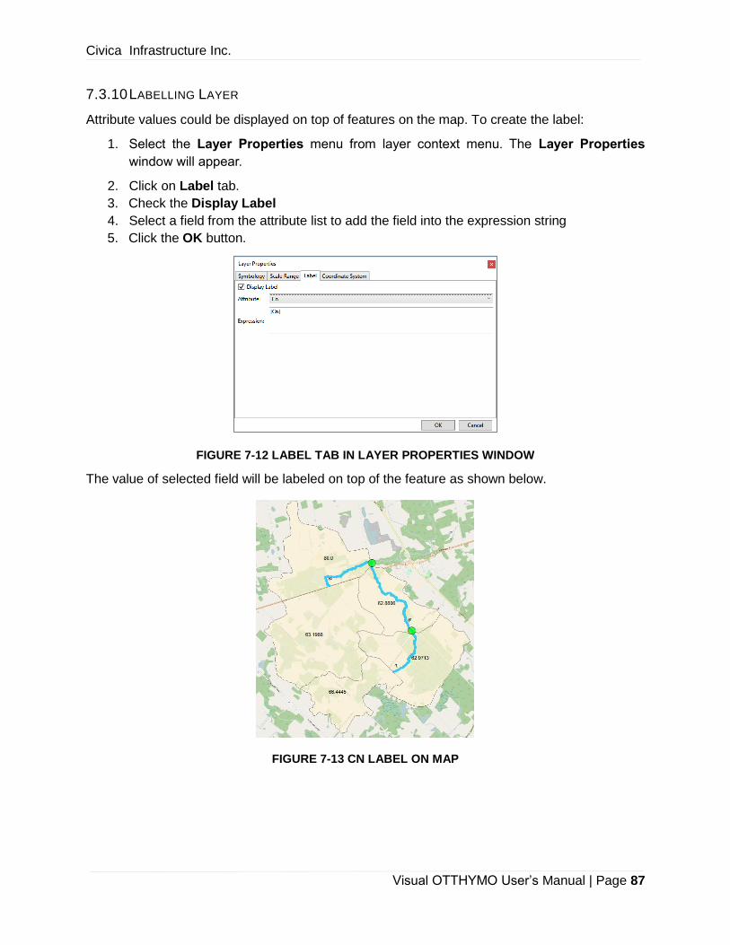
Civica Infrastructure Inc.
Visual OTTHYMO User’s Manual | Page 87
7.3.10 LABELLING LAYER
Attribute values could be displayed on top of features on the map. To create the label:
1. Select the Layer Properties menu from layer context menu. The Layer Properties
window will appear.
2. Click on Label tab.
3. Check the Display Label
4. Select a field from the attribute list to add the field into the expression string
5. Click the OK button.
FIGURE 7-12 LABEL TAB IN LAYER PROPERTIES WINDOW
The value of selected field will be labeled on top of the feature as shown below.
FIGURE 7-13 CN LABEL ON MAP
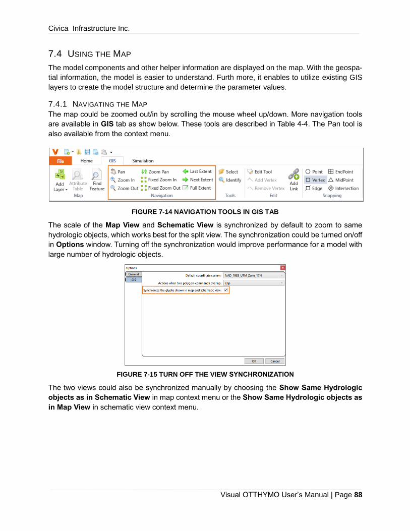
Civica Infrastructure Inc.
Visual OTTHYMO User’s Manual | Page 88
7.4 USING THE MAP
The model components and other helper information are displayed on the map. With the geospa-
tial information, the model is easier to understand. Furth more, it enables to utilize existing GIS
layers to create the model structure and determine the parameter values.
7.4.1 NAVIGATING THE MAP
The map could be zoomed out/in by scrolling the mouse wheel up/down. More navigation tools
are available in GIS tab as show below. These tools are described in Table 4-4. The Pan tool is
also available from the context menu.
FIGURE 7-14 NAVIGATION TOOLS IN GIS TAB
The scale of the Map View and Schematic View is synchronized by default to zoom to same
hydrologic objects, which works best for the split view. The synchronization could be turned on/off
in Options window. Turning off the synchronization would improve performance for a model with
large number of hydrologic objects.
FIGURE 7-15 TURN OFF THE VIEW SYNCHRONIZATION
The two views could also be synchronized manually by choosing the Show Same Hydrologic
objects as in Schematic View in map context menu or the Show Same Hydrologic objects as
in Map View in schematic view context menu.

Civica Infrastructure Inc.
Visual OTTHYMO User’s Manual | Page 89
FIGURE 7-16 VIEW SYNCHRONIZATION MENU IN MAP AND SCHEMATIC CONTEXT MENU
Note that the views are not synchronized when it’s not in split view model even the synchronization
is turned on. Please use the manual synchronization context menu when switching to another
view.
7.4.2 SELECTING FEATURES ON MAP
Features could be selected on map. To select features:
1. Click the Select button in GIS tab.
2. Click the feature on the map. The outline of the selected feature will be changed.
3. To add other features to the selection, hold the CTRL key and click on the feature.
4. To select features in a rectangle, drag to draw the rectangle on the map.
Similar as in Schematic View, certain hydrologic objects could be selected by using the
Selection context menu. These menus are described in 6.3.
FIGURE 7-17 SELECTION MENUES IN MAP CONTEXT MENU
For hydrological object layers, the hydrologic objects are also selected if the corresponding fea-
tures are selected.

Civica Infrastructure Inc.
Visual OTTHYMO User’s Manual | Page 90
7.4.3 CREATING HYDROLOGIC OBJECTS MANUALLY
VO provides tools to create hydrologic objects on map. Different from the Schematic View, the
geometry needs to be digitized on map before the objects could be created. To create a hydro-
logical object on map:
1. Turn on the base map layer for reference.
2. Configure the snapping environment in the GIS tab to snap certain point on existing
shapes. Their usage is described in Table 7-3. It could be changed anytime during the
digitization process. Notice that only Vertex is selected by default.
TABLE 7-3 SNAPPING TOOLS
Icon Command Icon Command
Point
Allows to snap to a point.
EndPoint
Allows to snap to the end point of
polyline or polygon.
Vertex
Allows to snap to the vertex.
MidPoint
Allows to snap to the middle point
of a polyline
Edge
Allows to snap along the
edge of polyline or polygon.
Intersection
Allows to snap to intersection of
two geometries
3. Specify the type of new hydrologic object by:
a. Dragging and dropping the hydrologic object icon from the toolbox to Map View.
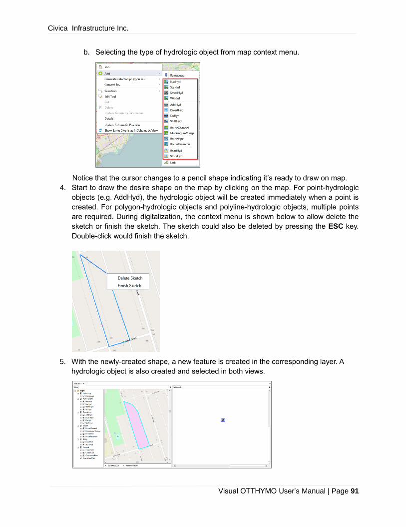
Civica Infrastructure Inc.
Visual OTTHYMO User’s Manual | Page 91
b. Selecting the type of hydrologic object from map context menu.
Notice that the cursor changes to a pencil shape indicating it’s ready to draw on map.
4. Start to draw the desire shape on the map by clicking on the map. For point-hydrologic
objects (e.g. AddHyd), the hydrologic object will be created immediately when a point is
created. For polygon-hydrologic objects and polyline-hydrologic objects, multiple points
are required. During digitalization, the context menu is shown below to allow delete the
sketch or finish the sketch. The sketch could also be deleted by pressing the ESC key.
Double-click would finish the sketch.
5. With the newly-created shape, a new feature is created in the corresponding layer. A
hydrologic object is also created and selected in both views.

Civica Infrastructure Inc.
Visual OTTHYMO User’s Manual | Page 92
7.4.4 CREATING HYDROLOGIC OBJECTS WITH GIS DATA
Existing GIS data could be utilized to define hydrologic objects. The data may be created from
DEM data using other hydrological analysis toolsets. These datasets usually have a catchment
layer, a stream layer and an outlet layer. They could be imported into VO and used to create
NasHyds/StandHyds, RouteChannels and AddHyds.
To create hydrologic objects from existing GIS layer:
1. Add existing GIS data using Add Feature Layer button in GIS tab. Move the layer on
top of base map layer and zoom to it using the Zoom to Layer context menu.
2. Select feature(s) in imported layers using the Select tool in GIS tab or map context
menu.
3. In map context menu, select the type of hydrologic object in Generate Selected
Geometry As menu. This is the type the new hydrologic object will be. Depending on the
type of selected features (point, polyline or polygon), some menu may be disabled as there
is no proper geometry for those hydrologic objects. In this case, no polyline feature is
selected, so RouteChannel, MuskingumCunge and RoutePipe is disabled.
4. A new hydrologic object will be created for each selected feature. The shape-based
parameters (e.g. area for catchments and length for channels) are automatically
calculated from the shape and all other parameters are using the default values.

Civica Infrastructure Inc.
Visual OTTHYMO User’s Manual | Page 93
7.4.5 LINKING HYDROLOGIC OBJECTS
Links between hydrologic objects could also be created in Map View. To create a link:
1. Click the Add Link button in GIS tab or choose the Add -> Link menu from the map
context menu. Notice the cursor changes to cross hair shape.
2. Move the cursor to the hydrologic object that will be the source of the link. Notice the
hydrologic object will flash with red color, which indicates the hydrologic object is eligible
as the link source. If the hydrologic object is not eligible, the hydrologic object won’t flash.
For example, a NasHyd which already has been linked to an AddHyd is not eligible as the
link source as it could only have one output link. The connection rules are given Table 6-3.
3. Click the desired hydrologic object to set it as the source of the link and move the cursor
to the hydrologic object it will be connected to. Notice that a red line will appear to connect
from the hydrologic object to the location of the cursor as shown below. This line
represents the link that will be added.

Civica Infrastructure Inc.
Visual OTTHYMO User’s Manual | Page 94
The starting point of the line is determined based on the shape of the hydrologic object.
For polygon-hydrologic object, the starting point will be the centroid of the polygon. For
polyline-hydrologic object, the starting point will be the middle point of the polyline. The
starting point of a point-hydrologic object will be where the point is located.
4. To select the destination object feature, move the cursor on top of that feature. If that
feature flashes, click to add the link. If the number of the input link of that hydrologic object
reaches the limitation, that hydrologic object won’t flash and the link can’t be added.
Same as the starting point, the ending point of the link is also determined by the shape of
that hydrologic object. Middle point is used for polylines.
A new feature is added to CatchmentLine layer for the new link as shown below. The
symbol may be different based on your settings.
Once the link is added, the output property of the starting hydrologic object is updated
automatically to the output hydrologic object and a link is also added in the schematic view
as shown blow.

Civica Infrastructure Inc.
Visual OTTHYMO User’s Manual | Page 95
5. To star over the process in the middle, press the ESC key. The starting point will be
cleared.
6. To remove the link, click the edit tool, select the link on map and press DELETE key. A
confirm window would appear as shown below. Click Yes to confirm the deletion. The link
in the schematic view will also be removed and the outlet property will be set to empty.
7.4.6 ASSIGNING GEOMETRY TO EXISTING HYDROLOGICAL OBJECTS
Hydrologic objects don’t have geospatial location information when 1) they are created on canvas
or 2) they are imported from and older model. To take advantage of GIS functions, the geospatial
location information could be assigned to hydrological objects. To do this:
1. Click the Assign Geometry button in the GIS tab. The Assign Geometry window will
appear. By default, the window lists all hydrologic objects that have no associated geometry.
It can also show all hydrologic objects by unchecking Filter Commands with Geometries.
2. To assign a manually-created geometry, click the Assign New Geometry button at bottom
and the cursor changes to a pencil. Follow the same procedure as in 4.2.1 to create the
geometry. Once the geometry is successfully created, it will be assigned to the selected hy-
drologic object.
3. To assign exiting geometry to selected hydrologic object, add the data layer first and select
the geometry on map. And then select the correct hydrologic object in the list and click Assign
Selected Geometry button at the bottom.

Civica Infrastructure Inc.
Visual OTTHYMO User’s Manual | Page 96
7.4.7 MOVING, EDITING AND DELETING HYDROLOGIC OBJECTS
The shape of the hydrologic object features could be edited and deleted on map. To do this:
1. Select Edit Tool in GIS tab or map context menu.
2. Select the hydrologic object feature on map.
3. To move a feature, move the cursor on top of the selected features and then hold the left
button to drag it to the new location. When the moving is underway, a new shape is shown
to represent what it will look like after the move. Release the left button to confirm the
move. Note that moving is not allowed when more than one hydrologic objects are
selected.
For polygon-hydrologic objects, the new shape may cover, cut or clip other hydrologic
objects. This is not allowed. If that happens, a warning message shows up and the new
shape will be rejected.

Civica Infrastructure Inc.
Visual OTTHYMO User’s Manual | Page 97
If the new shape clips other hydrologic objects like the one shown below, the behaviour is
defined in Options window. The default behaviour is Reject, which would reject the
change. If it’s set to Clip, the affected hydrologic objects would be clipped and the area is
updated. This setting also applies when a new polygon hydrologic object feature is created
and an existing polygon hydrologic object features is changed by moving, adding or
removing a vertex.
As moving a polygon-hydrologic objects may change other hydrologic objects, it’s
generally not recommended to do so.
4. To change the shape of the hydrologic object, double-click it on the map to show all the
vertices. Move cursor on top of one of them and drag it to a new location.

Civica Infrastructure Inc.
Visual OTTHYMO User’s Manual | Page 98
5. Vertices could be added or removed by using Add Vertex and Remove Vertex in
GIS tab. For Add Vertex, set the snapping properly to make the new vertex more accurate.
Click on the map, a new vertex is added at that location and the shape is changed
accordingly. For Remove Vertex, the vertex will be removed by clicking on it. Note that
these two tools are only available when a polygon or a polyline is selected using the Edit
tool.
6. To delete selected hydrologic object(s), press the DELETE key or choose Delete on map
context menu. A warning window appears to provide the opportunity to confirm the
deletion. Click Yes to confirm the deletion.
7.4.8 CUTTING POLYGON-HYDROLOGIC OBJECTS
In some cases, a polygon-hydrologic object needs to be split into several smaller ones, e.g. part
of NasHyd is developed and the imperviousness surpass 20%. To do this:
1. Select the polygon-hydrologic object first and select Cut from context menu. Notice the
cursor change to a pencil.
2. Setup the snapping environment if necessary to snap to desired points.
3. Draw the polyline that will be the boundary between new hydrologic objects and double
click to finish the sketch. If the polygon could be cut into pieces, new hydrologic objects
will be created.
If the polyline couldn’t cut the polygon into pieces, a warning window will appear.

Civica Infrastructure Inc.
Visual OTTHYMO User’s Manual | Page 99
7.5 UPDATING HYDROLOGIC OBJECTS LOCATION IN SCHEMATIC VIEW
The location of hydrologic objects in schematic view could be determined based on their geospa-
tial location on map. Doing so would make hydrologic objects locate in similar location in sche-
matic view, which would make comparison easier.
To update the location, choose the Update Schematic Position context menu and click Yes on
the confirmation window. The location of all hydrologic objects would be updated.
For some models with large number of hydrologic objects, the location of few hydrologic objects
may not that accurate. They need to be adjusted manually.
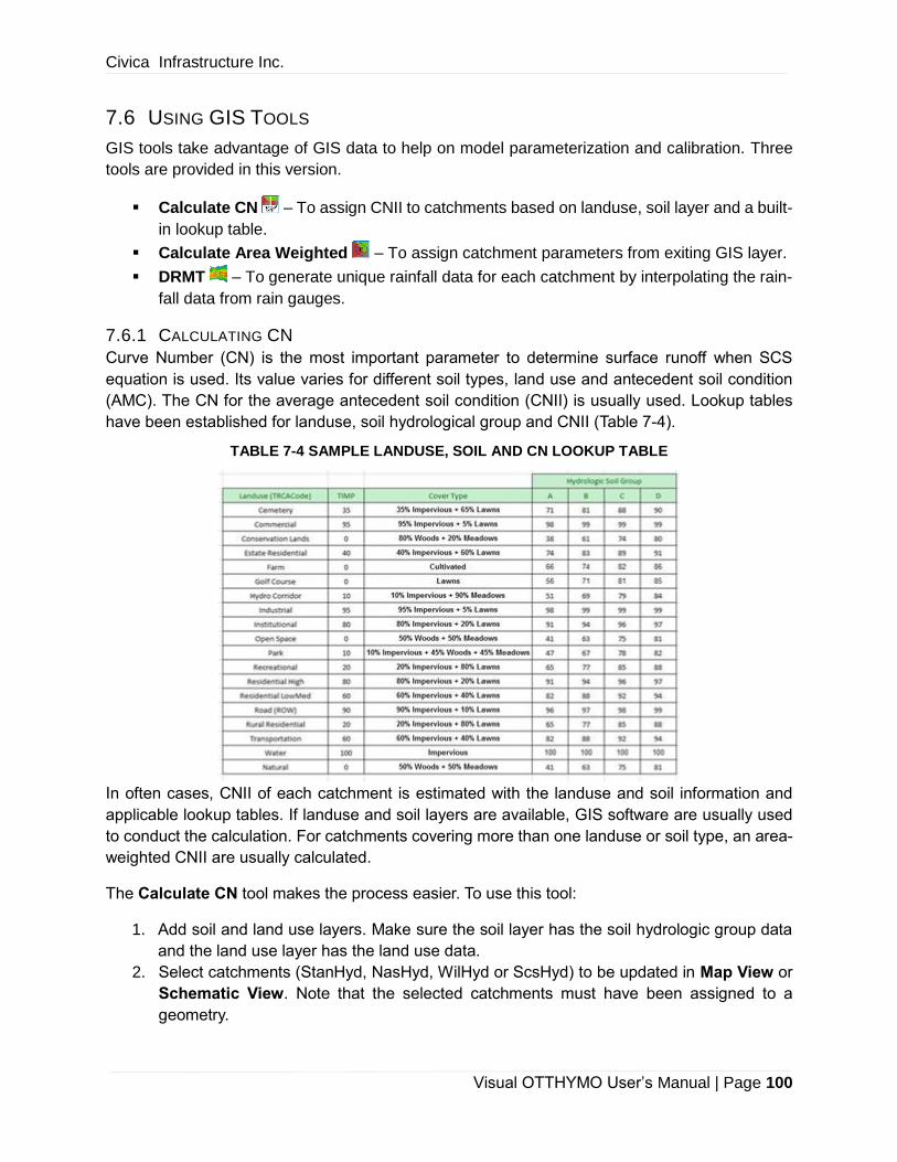
Civica Infrastructure Inc.
Visual OTTHYMO User’s Manual | Page 100
7.6 USING GIS TOOLS
GIS tools take advantage of GIS data to help on model parameterization and calibration. Three
tools are provided in this version.
▪ Calculate CN – To assign CNII to catchments based on landuse, soil layer and a built-
in lookup table.
▪ Calculate Area Weighted – To assign catchment parameters from exiting GIS layer.
▪ DRMT – To generate unique rainfall data for each catchment by interpolating the rain-
fall data from rain gauges.
7.6.1 CALCULATING CN
Curve Number (CN) is the most important parameter to determine surface runoff when SCS
equation is used. Its value varies for different soil types, land use and antecedent soil condition
(AMC). The CN for the average antecedent soil condition (CNII) is usually used. Lookup tables
have been established for landuse, soil hydrological group and CNII (Table 7-4).
TABLE 7-4 SAMPLE LANDUSE, SOIL AND CN LOOKUP TABLE
In often cases, CNII of each catchment is estimated with the landuse and soil information and
applicable lookup tables. If landuse and soil layers are available, GIS software are usually used
to conduct the calculation. For catchments covering more than one landuse or soil type, an area-
weighted CNII are usually calculated.
The Calculate CN tool makes the process easier. To use this tool:
1. Add soil and land use layers. Make sure the soil layer has the soil hydrologic group data
and the land use layer has the land use data.
2. Select catchments (StanHyd, NasHyd, WilHyd or ScsHyd) to be updated in Map View or
Schematic View. Note that the selected catchments must have been assigned to a
geometry.
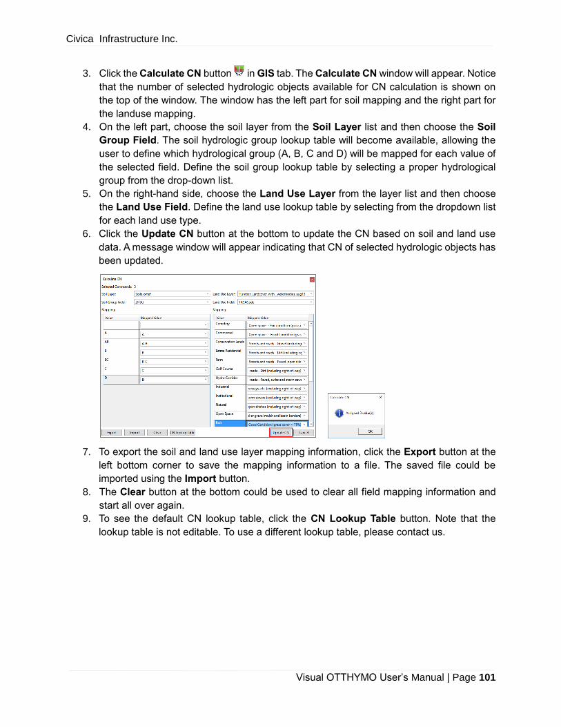
Civica Infrastructure Inc.
Visual OTTHYMO User’s Manual | Page 101
3. Click the Calculate CN button in GIS tab. The Calculate CN window will appear. Notice
that the number of selected hydrologic objects available for CN calculation is shown on
the top of the window. The window has the left part for soil mapping and the right part for
the landuse mapping.
4. On the left part, choose the soil layer from the Soil Layer list and then choose the Soil
Group Field. The soil hydrologic group lookup table will become available, allowing the
user to define which hydrological group (A, B, C and D) will be mapped for each value of
the selected field. Define the soil group lookup table by selecting a proper hydrological
group from the drop-down list.
5. On the right-hand side, choose the Land Use Layer from the layer list and then choose
the Land Use Field. Define the land use lookup table by selecting from the dropdown list
for each land use type.
6. Click the Update CN button at the bottom to update the CN based on soil and land use
data. A message window will appear indicating that CN of selected hydrologic objects has
been updated.
7. To export the soil and land use layer mapping information, click the Export button at the
left bottom corner to save the mapping information to a file. The saved file could be
imported using the Import button.
8. The Clear button at the bottom could be used to clear all field mapping information and
start all over again.
9. To see the default CN lookup table, click the CN Lookup Table button. Note that the
lookup table is not editable. To use a different lookup table, please contact us.

Civica Infrastructure Inc.
Visual OTTHYMO User’s Manual | Page 102
7.6.2 CALCULATING AREA WEIGHTED
In some cases, model parameters are available in GIS layers. The Calculate Area Weighted tool
reads the parameter values, calculate the area weighted value if necessary and then assign to
catchments. The imperviousness (TIMP and XIMP) and initial abstraction are two parameters that
could utilize this tool. To use this tool:
1. Add the GIS layer that has the parameter information.
2. Select catchments whose parameter will be updated.
3. Click the Calculate Area Weighted button located in the GIS tab. The Calculate Area
Weighted Parameter window will appear. Notice that the number of selected catchments
is shown at the top of the window.
4. Choose Parameter to Calculate from the drop-down menu. In this case, only StandHyd
parameters are shown here as only StanHyds are selected. We want to use Timp this
time.
5. Choose the Source Layer and the Source Field, where the parameter values will be
retrieved. The source layer should be a polygon layer and the source field could be any
type. In this case, we choose Percentimp, which is a numerical field indicating the
percentage of impervious area in the polygon.
6. Define the field mapping to map all the field values to the desired parameter value.
7. Click the Update button at the bottom of the window. A message window will appear,
indicating that the parameter of selected hydrologic objects has been updated.
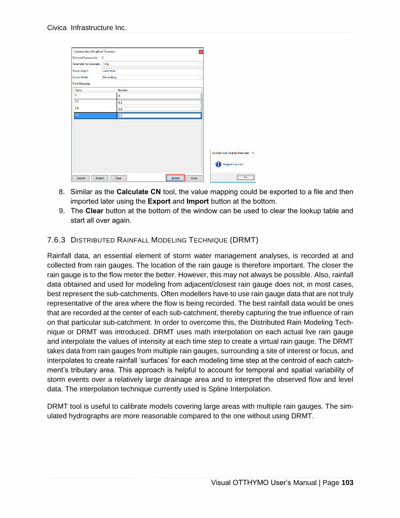
Civica Infrastructure Inc.
Visual OTTHYMO User’s Manual | Page 103
8. Similar as the Calculate CN tool, the value mapping could be exported to a file and then
imported later using the Export and Import button at the bottom.
9. The Clear button at the bottom of the window can be used to clear the lookup table and
start all over again.
7.6.3 DISTRIBUTED RAINFALL MODELING TECHNIQUE (DRMT)
Rainfall data, an essential element of storm water management analyses, is recorded at and
collected from rain gauges. The location of the rain gauge is therefore important. The closer the
rain gauge is to the flow meter the better. However, this may not always be possible. Also, rainfall
data obtained and used for modeling from adjacent/closest rain gauge does not, in most cases,
best represent the sub-catchments. Often modellers have to use rain gauge data that are not truly
representative of the area where the flow is being recorded. The best rainfall data would be ones
that are recorded at the center of each sub-catchment, thereby capturing the true influence of rain
on that particular sub-catchment. In order to overcome this, the Distributed Rain Modeling Tech-
nique or DRMT was introduced. DRMT uses math interpolation on each actual live rain gauge
and interpolate the values of intensity at each time step to create a virtual rain gauge. The DRMT
takes data from rain gauges from multiple rain gauges, surrounding a site of interest or focus, and
interpolates to create rainfall ‘surfaces’ for each modeling time step at the centroid of each catch-
ment’s tributary area. This approach is helpful to account for temporal and spatial variability of
storm events over a relatively large drainage area and to interpret the observed flow and level
data. The interpolation technique currently used is Spline Interpolation.
DRMT tool is useful to calibrate models covering large areas with multiple rain gauges. The sim-
ulated hydrographs are more reasonable compared to the one without using DRMT.

Civica Infrastructure Inc.
Visual OTTHYMO User’s Manual | Page 104
7.6.3.1 ADDING RAIN GAUGES
To have a proper rainfall surface, minimum three rain gauges are required. Adding a rain gauge
is similar to adding other point hydrologic objects (e.g. AddHyd). To add rain gauges on map:
1. Select Add->Rainguage in map context menu.
2. Click on the map to add the rain gauge.
3. Set the storm index pointing to the rainfall data in a rain group. It’s recommended to use
same storm index in different rain groups to avoid changing the storm index after switch
between rain groups. In this context, the rain group is a collection of rainfalls happening
at the same time but at different locations. A good practise is to name the rain group with
the rainfall time range and name the rainfall data with rain gauge name.
7.6.3.2 USING DRMT TOOL
To use the DRMT tool interpolate the rainfall for each catchment:
1. Click the DRMT tool in GIS tab. The Generate DRMT window will appear. The number
of selected catchments is given at top of the window. If no catchment is selected, it will
apply to all catchments.
2. DRMT tool uses a two-dimensional minimum curvature spline technique to generate the
rainfall intensity surface. The parameters in Generate DRMT window are described in
following table. Most of the parameters have a default value.

Civica Infrastructure Inc.
Visual OTTHYMO User’s Manual | Page 105
Parameter Description
Input Rain Select the rain group as the hyetograph data source for rain
gauges.
Output cell size
The cell size (m) at which the output raster will be created.
By default, it is the shorter of the width or the height of the
extent of the selected rain gauges, divided by 250.
Spline Type
The type of spline to be used. It can be REGULARIZED or
TENSION. REGULARIZED yields a smooth surface and
smooth first derivatives. TENSION tunes the stiffness of the
interpolant according to the character of the modeled phe-
nomenon. By default, REGULARIZED is used.
Weight
Parameter influencing the character of the surface interpola-
tion. When the REGULARIZED option is used, it defines the
weight of the third derivatives of the surface in the curvature
minimization expression. If the TENSION option is used, it
defines the weight of tension. The default value is 0.1.
Number of points The number of points per region used for local approximation.
The default value is 12.
Intensity over catch-
ment
The method to calculate the rain fall intensity over catchment
using the rainfall surface. It can be centroid or catchment
average. Centroid uses the rain fall intensity at the catch-
ment polygon centroid. Catchment Average calculates the
average rain fall intensity over the catchment. The centroid
is the default value.
Rainfall raster output
path
Folder for generated rainfall surface raster data
Selected rain gauges Rain gauges whose location will be used for the interpolation.
All rain gauges are selected by default.
3. Choose the rain group from the Input Rain drop-down list and change other parameters
if necessary. If there are more than three rain gauges, some rain gauges could be removed
from the selected list by drag-and-drop.
4. Click OK button at the bottom. The GeoProcessing window appears to show the progress
and a message window appears once the process is done.

Civica Infrastructure Inc.
Visual OTTHYMO User’s Manual | Page 106
5. After the process finish, a new rain group is created. It has 5 hyetographs, which are
corresponding to the 5 selected subcatchments. As they are generated from the
interpolated surface, each hyetograph is unique. Notice that the icon for DRMT-generated
rain group is different with those created manually . A capital letter “D” appears on
the top right corner to represent DRMT. These rain groups are not editable.
6. The DRMT-generated rain groups could be used to run the simulation as other rain groups.
In Batch Run window through the Run button in Simulation tab, select the rain group
from the Rain drop down list as shown below. The corresponding hyetographs will be
automatically assigned to hydrograph commands.
7.7 TURNING OFF MAP FUNCTIONS
By default, VO will load map functions when an ArcGIS license is available. This could be changed
in Options window as shown in Figure 7-18. Uncheck the Use GIS option in General tab. Note

Civica Infrastructure Inc.
Visual OTTHYMO User’s Manual | Page 107
that this option only appear when ArcGIS license is available and the change will take effect after
the program is restarted.
FIGURE 7-18 TURNING OFF GIS IN OPTIONS WINDOW

Civica Infrastructure Inc.
Visual OTTHYMO User’s Manual | Page 108
8 WORKING WITH CLIMATE LIBRARY
Climate Library is a local climate data library with the ability to share with others. Shipped with
standard design and regional storm used in Toronto and Region Conversion Authority (TRCA), it
could be expanded with any project related climate data.
The climate data in Climate Library includes Intensity-Duration-Frequency (IDF), design storm,
regional storm, rain gauge, temperature gauge, evaporation gauge, precipitation time series, tem-
perature time series and evaporation time series. More climate data will be added in later ver-
sions.
The climate data is organized in a folder-like structure supporting unlimited levels. The Library
Explorer in the Climate Library provides similar functionality as the File Explorer in Windows
operation system.
With current version, the climate data is either entered or imported from a file. Database connec-
tion will be added in the later version to grab data from existing database.
Review agencies may find Climate Library is a good way to distribute the design storms required
in the development submissions. Modellers and engineers may find themselves save time by
avoiding using file-based climate files.
8.1 OPENING CLIMATE LIBRARY
To open Climate Library, use the Climate Library button in Simulation tab or the Project
Manager tool bar.
The Climate Library has three (3) components: Toolbar, Library Explorer and Main View. The
Toolbar is on the top where buttons are placed in different groups. The Library Explorer, a tree
view of all items in the library, is located on the left. Each item has a unique icon and context
menu. The Main View displays the information of selected item. It changes depending on the
type of the items.

Civica Infrastructure Inc.
Visual OTTHYMO User’s Manual | Page 109
FIGURE 8-1 OPENING CLIMATE LIBRARY
8.2 TOOLBAR
The buttons in the toolbar are described in Table 8-1. Most of them are also available through the
context menu in Library Explorer.
8.3 LIBRARY EXPLORER
The Library Explorer shows all items in a tree view structure.
8.3.1 ODER OF ITEMS
Items of different types in one group are organized in a certain order as described below. Items
with higher order will appear before items with lower order. Items of same type are arranged
alphabetically by name.
1. Sub-group
2. Rain Gauge
3. IDF Group
4. Manual Input Design Storm
5. Read-in Design Storm
6. Chicago Design Storm
7. Mass Design Storm
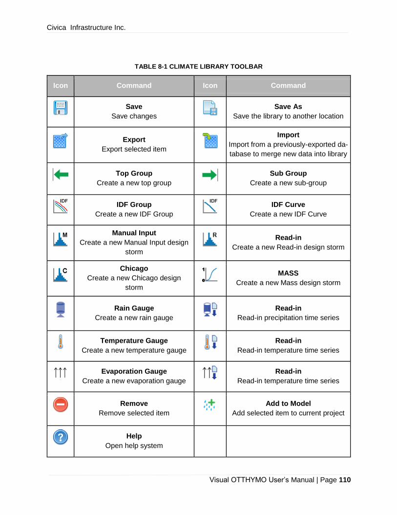
Civica Infrastructure Inc.
Visual OTTHYMO User’s Manual | Page 110
TABLE 8-1 CLIMATE LIBRARY TOOLBAR
Icon Command Icon Command
Save
Save changes Save As
Save the library to another location
Export
Export selected item
Import
Import from a previously-exported da-
tabase to merge new data into library
Top Group
Create a new top group Sub Group
Create a new sub-group
IDF Group
Create a new IDF Group IDF Curve
Create a new IDF Curve
Manual Input
Create a new Manual Input design
storm
Read-in
Create a new Read-in design storm
Chicago
Create a new Chicago design
storm
MASS
Create a new Mass design storm
Rain Gauge
Create a new rain gauge Read-in
Read-in precipitation time series
Temperature Gauge
Create a new temperature gauge Read-in
Read-in temperature time series
Evaporation Gauge
Create a new evaporation gauge Read-in
Read-in temperature time series
Remove
Remove selected item Add to Model
Add selected item to current project
Help
Open help system

Civica Infrastructure Inc.
Visual OTTHYMO User’s Manual | Page 111
8.3.2 ICONS
In Library Explorer, icons are used to identify different items in the library as shown in Table 8-2.
TABLE 8-2 LIBRARY EXPLORER ICONS
Icon Data Type Icon Data Type
Group
IDF Group IDF Curve
Manual Input Design Storm Read-in Design Storm
Chicago Design Storm Mass Design Storm
SCS Type II Design Storm AES Design Storm
Rain Gauge Read-in Measured Storm
Temperature Gauge Temperature Data
Evaporation Gauge Evaporation Data
8.3.3 CONTEXT MENU
Context menus in Library Explorer is content-sensitive. An example is given below.
8.3.4 DRAG AND DROP
The items in Library Explorer supports drag-and-drop for various functions based on the type of
source and destination item. Examples are:
▪ Move item from one group to another
▪ Apply IDF to Chicago design storm
▪ Add design storm and temperature data to Project Manager.

Civica Infrastructure Inc.
Visual OTTHYMO User’s Manual | Page 112
8.4 MAIN VIEW
The items in Climate Library is displayed and edited in the Main View. The Main View changes
depending on the type of the item. The view for IDF group, Chicago design storm, MASS design
storm and temperature data is given below.
FIGURE 8-2 CLIMATE LIBRARY MAIN VIEW
8.5 ADDING NEW ITEMS
Items could be added to the library by using the buttons in the Toolbar or the context menu in
Library Explorer.
IDF Group Chicago Design Storm
MASS Design Storm Temperature Data
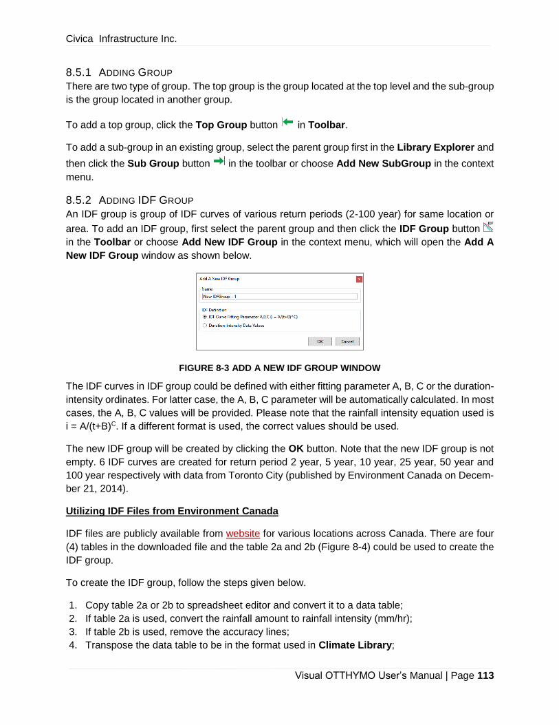
Civica Infrastructure Inc.
Visual OTTHYMO User’s Manual | Page 113
8.5.1 ADDING GROUP
There are two type of group. The top group is the group located at the top level and the sub-group
is the group located in another group.
To add a top group, click the Top Group button in Toolbar.
To add a sub-group in an existing group, select the parent group first in the Library Explorer and
then click the Sub Group button in the toolbar or choose Add New SubGroup in the context
menu.
8.5.2 ADDING IDF GROUP
An IDF group is group of IDF curves of various return periods (2-100 year) for same location or
area. To add an IDF group, first select the parent group and then click the IDF Group button
in the Toolbar or choose Add New IDF Group in the context menu, which will open the Add A
New IDF Group window as shown below.
FIGURE 8-3 ADD A NEW IDF GROUP WINDOW
The IDF curves in IDF group could be defined with either fitting parameter A, B, C or the duration-
intensity ordinates. For latter case, the A, B, C parameter will be automatically calculated. In most
cases, the A, B, C values will be provided. Please note that the rainfall intensity equation used is
i = A/(t+B)C. If a different format is used, the correct values should be used.
The new IDF group will be created by clicking the OK button. Note that the new IDF group is not
empty. 6 IDF curves are created for return period 2 year, 5 year, 10 year, 25 year, 50 year and
100 year respectively with data from Toronto City (published by Environment Canada on Decem-
ber 21, 2014).
Utilizing IDF Files from Environment Canada
IDF files are publicly available from website for various locations across Canada. There are four
(4) tables in the downloaded file and the table 2a and 2b (Figure 8-4) could be used to create the
IDF group.
To create the IDF group, follow the steps given below.
1. Copy table 2a or 2b to spreadsheet editor and convert it to a data table;
2. If table 2a is used, convert the rainfall amount to rainfall intensity (mm/hr);
3. If table 2b is used, remove the accuracy lines;
4. Transpose the data table to be in the format used in Climate Library;
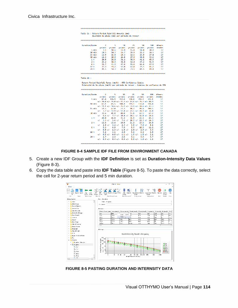
Civica Infrastructure Inc.
Visual OTTHYMO User’s Manual | Page 114
FIGURE 8-4 SAMPLE IDF FILE FROM ENVIRONMENT CANADA
5. Create a new IDF Group with the IDF Definition is set as Duration-Intensity Data Values
(Figure 8-3).
6. Copy the data table and paste into IDF Table (Figure 8-5). To paste the data correctly, select
the cell for 2-year return period and 5 min duration.
FIGURE 8-5 PASTING DURATION AND INTERNSITY DATA

Civica Infrastructure Inc.
Visual OTTHYMO User’s Manual | Page 115
8.5.3 ADDING IDF CURVE
It’s necessary to add a new IDF curve if the desired return period doesn’t present in the IDF group.
It’s could be added by clicking the IDF curve button in the Toolbar or choosing the Add New
IDF Curve menu in the IDF Group context menu. The return period of the new IDF curve is 0 and
needs to be edited later.
8.5.4 ADDING DESIGN STORM
There are four ways to create a design storm in Climate Library which are corresponding to
different scenarios.
1. Manual Input could be used for the case where the design storm will be created from
scratch. It gives the flexibility to add, insert, modify and delete the time series data directly.
Although it also supports copy-and-paste from other source, it's not recommended to use
manual input for that case. Read-in should be used instead.
2. Read-in is design for an existing design storm, which may be exported from another de-
sign storm tool or modelling software. Two file formats are supported (stm an csv).
3. Chicago is used to create a Chicago design storm based on given parameters including
IDF curve. It's often used for cases where model needs to run on Chicago design storms
from IDF curves with different return period. It's recommended to add the IDF information
into the library first and then create the design storm.
4. Mass is used when a mass curve file and total precipitation is available. Examples are
SCS Type II and AES design storms.
5. SCS Type II is used to create a 6-hr, 12-hr or 24-hr SCS Type II design storm.
6. AES is used to create a 1-hr AES design storm.
To create these design storms, click the corresponding button in toolbar or choose the corre-
sponding menu in the context menu as shown in Figure 8-6.
FIGURE 8-6 NEW DESIGN STORM BUTTON AND CONTEXT MENU

Civica Infrastructure Inc.
Visual OTTHYMO User’s Manual | Page 116
New manual input and Chicago design storms will be added immediately and set as the active
item. A window will appear for Read-in and MASS design storm for user to preview the data before
it’s added into the library.
Chicago, SCS Type II and AES design storms could also be created based-on IDF Group as
shown in Figure 8-7. The design storms are created for each return period in the IDF Group.
FIGURE 8-7 NEW DESIGNS STORMS CONTEXT MENU BASED-ON IDF GROUP
8.5.4.1 NEW READ-IN DESIGN STORM
The window for new read-in storm is shown in Figure 8-8. It allows to give a name and browse
the data file for preview.
Click the Browse… button in the window to browse the data file to display it in the Data Preview
area at the bottom as shown below. It supports the STM file and CSV file.
If Use File Name is checked, the file name will be set as the name of the new read-in design
storm. If you are satisfied with the data, click OK button to create the design storm in the library.
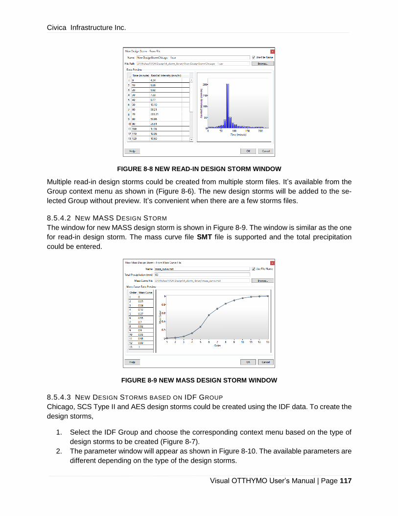
Civica Infrastructure Inc.
Visual OTTHYMO User’s Manual | Page 117
FIGURE 8-8 NEW READ-IN DESIGN STORM WINDOW
Multiple read-in design storms could be created from multiple storm files. It’s available from the
Group context menu as shown in (Figure 8-6). The new design storms will be added to the se-
lected Group without preview. It’s convenient when there are a few storms files.
8.5.4.2 NEW MASS DESIGN STORM
The window for new MASS design storm is shown in Figure 8-9. The window is similar as the one
for read-in design storm. The mass curve file SMT file is supported and the total precipitation
could be entered.
FIGURE 8-9 NEW MASS DESIGN STORM WINDOW
8.5.4.3 NEW DESIGN STORMS BASED ON IDF GROUP
Chicago, SCS Type II and AES design storms could be created using the IDF data. To create the
design storms,
1. Select the IDF Group and choose the corresponding context menu based on the type of
design storms to be created (Figure 8-7).
2. The parameter window will appear as shown in Figure 8-10. The available parameters are
different depending on the type of the design storms.
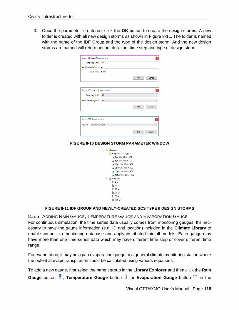
Civica Infrastructure Inc.
Visual OTTHYMO User’s Manual | Page 118
3. Once the parameter is entered, click the OK button to create the design storms. A new
folder is created with all new design storms as shown in Figure 8-11. The folder is named
with the name of the IDF Group and the type of the design storm. And the new design
storms are named will return period, duration, time step and type of design storm.
FIGURE 8-10 DESIGN STORM PARAMETER WINDOW
FIGURE 8-11 IDF GROUP AND NEWLY-CREATED SCS TYPE II DESIGN STORMS
8.5.5 ADDING RAIN GAUGE, TEMPERATURE GAUGE AND EVAPORATION GAUGE
For continuous simulation, the time series data usually comes from monitoring gauges. It’s nec-
essary to have the gauge information (e.g. ID and location) included in the Climate Library to
enable connect to monitoring database and apply distributed rainfall models. Each gauge may
have more than one time-series data which may have different time step or cover different time
range.
For evaporation, it may be a pan evaporation gauge or a general climate monitoring station where
the potential evapotranspiration could be calculated using various equations.
To add a new gauge, first select the parent group in the Library Explorer and then click the Rain
Gauge button , Temperature Gauge button or Evaporation Gauge button in the

Civica Infrastructure Inc.
Visual OTTHYMO User’s Manual | Page 119
Toolbar. For evaporation gauge, it’s necessary to specify the type of the data type. It could be
lake evaporation, pan evaporation or potential evapotranspiration.
FIGURE 8-12 EVAPORATION GAUGE VIEW
8.5.6 ADDING PRECIPITATION, TEMPERATURE AND EVAPORATION DATA
The monitoring precipitation, temperature and evaporation data is added to corresponding gauges
from a data file. To do this:
1. Select the gauge first and then click the proper Read-in button in the Toolbar.
2. In the New Monitored Data window, click the Browse… button in the window to browse
the data file to display it in the Data Preview area at the bottom. If Use File Name is
checked, the file name will be set as the name of the data item.
3. If you are satisfied with the data, click OK button to add the data item to the library.
The data file should be in a simple CSV file with first column as the time and the second column
as the data value. The first row is treated as the column name and will be ignored.
The data gap will be detected and filled. The precipitation will set as zero (0) and the temperature
and evaporation will be set as the one in previous time step.
Although data of any time step could be added to the library, the continuous simulation only sup-
ports certain time steps. For precipitation, it’s 5min, 10min, 15min, 20min, 1hr and 1day. For tem-
perature and evaporation, it’s 1day.
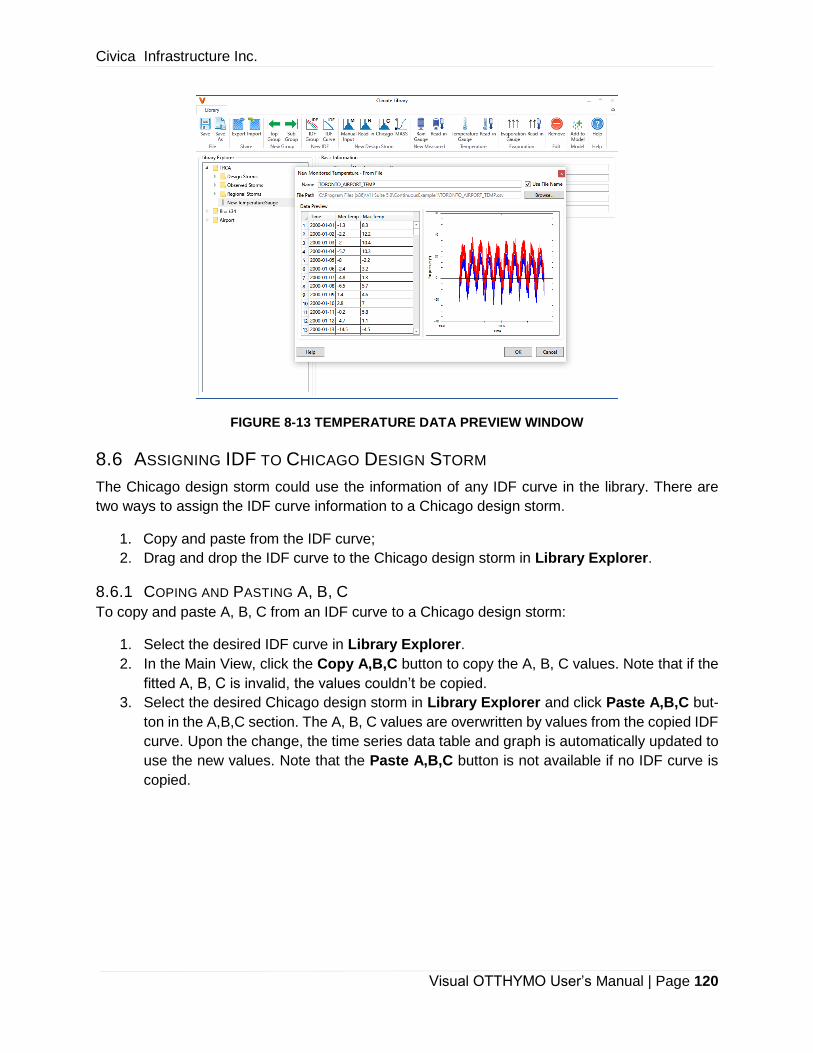
Civica Infrastructure Inc.
Visual OTTHYMO User’s Manual | Page 120
FIGURE 8-13 TEMPERATURE DATA PREVIEW WINDOW
8.6 ASSIGNING IDF TO CHICAGO DESIGN STORM
The Chicago design storm could use the information of any IDF curve in the library. There are
two ways to assign the IDF curve information to a Chicago design storm.
1. Copy and paste from the IDF curve;
2. Drag and drop the IDF curve to the Chicago design storm in Library Explorer.
8.6.1 COPING AND PASTING A, B, C
To copy and paste A, B, C from an IDF curve to a Chicago design storm:
1. Select the desired IDF curve in Library Explorer.
2. In the Main View, click the Copy A,B,C button to copy the A, B, C values. Note that if the
fitted A, B, C is invalid, the values couldn’t be copied.
3. Select the desired Chicago design storm in Library Explorer and click Paste A,B,C but-
ton in the A,B,C section. The A, B, C values are overwritten by values from the copied IDF
curve. Upon the change, the time series data table and graph is automatically updated to
use the new values. Note that the Paste A,B,C button is not available if no IDF curve is
copied.

Civica Infrastructure Inc.
Visual OTTHYMO User’s Manual | Page 121
FIGURE 8-14 COPY AND PAST IDF CURVE A, B, C
8.6.2 DRAGGING AND DROPPING IDF CURVE TO CHICAGO DESIGN STORM
To use drag-and-drop to assign the IDF curve information to a Chicago design storm:
1. Select the desired IDF curve in Library Explorer.
2. Keep the left mouse button pressed and drag it over the Chicago design storm in Library
Explorer. Notice that the mouse cursor changes to the one shown below, which indicates
the IDF curve information will be copied to the Chicago design storm.
3. Release the mouse button to assign A, B, C values to the Chicago design storm. Notice
the A, B, C values change and the time series are updated automatically.
FIGURE 8-15 DRAG-AND-DROP IDF CURVE TO CHICAGO DESIGN STORM
8.7 SHARING
Climate Library sharing is necessary to:
▪ Make sure the required IDF, design storm and time series data is used;
▪ Save time on prepare and import the data file.

Civica Infrastructure Inc.
Visual OTTHYMO User’s Manual | Page 122
Climate Library can share any part of the library. An item and its child items will be exported to
a separated database, which could be merged to other database with the structure unchanged.
Single items (e.g. design storm) could also be exported to data files.
8.7.1 EXPORTING
To export an item (and its children):
1. Select it in Library Explorer and click the Export button in the toolbar or choose the
Export menu in the context menu.
2. In the Save As window, change the default name and file format and then click Save. The
default output format is SQLite database.
Export function is used to export a branch of the library. To export the whole database, click the
Save As button in the toolbar and follow the same procedure.
8.7.2 IMPORTING
To import data from an exported database, click the Import button in the Toolbar. Browse the
right file in the Open window and click OK.
Importing merges the two databases together by only adding different items. Not all the data will
be imported into the local library. If the same structure with the same name already exists in the
same level, the existing item will be kept. For example, if a top group named Toronto exists in
both local library and the imported database, no new group is created and the existing one will be
used. These processes will be applied to all items in the imported library.
The process is demonstrated in Figure 8-16. A merged library is generated based on the local
library and the imported library. In this case, Group 1 and IDF Group 1 exists in both libraries. The
one in the local library will be kept without any change even the one in imported database is
different. Sub-group 2 and Design Storm 3 doesn't exist in local library and is added into the final
merged library.

Civica Infrastructure Inc.
Visual OTTHYMO User’s Manual | Page 123
FIGURE 8-16 CLIMATE LIBRARY MERGE DIAGRAM
8.8 ADDING CLIMATE DATA TO MODEL
Climate Library acts as the sole source of climate data for model. The climate data (rain, tem-
perature and evaporation) could be added to the working model by 1) using the Add to model
button/menu, 2) using Add All Design Storms to Project menu or 2) drag-and-drop.
To use the Add to model button/menu:
1. Select the climate data in the Library Explorer;
2. Click the Add to Model button in the toolbar or choose the Add to model… menu in
the context menu;
3. The Add Storm(s) to Rain Group window will appear. The first one allows to choose one
of the existing rain groups to add the design storm. The second one would create a new
rain group with the given name.
4. Click OK to add the design storm to the model. The new rain group will appear in Project
Manager.
Civica Infrastructure Inc.
Visual OTTHYMO User’s Manual | Page 124
To use Add All Design Storms to Project Menu
Design storms in a group could be added to a model at once. To do this, select the group in the
Library Explorer and choose the Add All Design Storm to Project from the context menu as
shown below. All the design storms will be added to the model and the run group is also created
for each design storm.
To use the drag-and-drop:
1. Make sure the Project Manager is visible and not covered by Climate Library window.
2. Select the desired climate data in the Library Explorer
3. To create a new climate data group, drag it to the corresponding section in Project Man-
ager:
• for design storm and long-term precipitation
• for temperature
• for evaporation.

Civica Infrastructure Inc.
Visual OTTHYMO User’s Manual | Page 125
4. To add the climate data to an existing climate date group, drag it to existing rain group
, temperature group or evaporation group in Project Manager;
5. The cursor would change to indicate the climate data could be added to current location.
6. Release mouse to finish the operation. The climate data will be added current location
and appears in Project Manager.
Certain rules apply when adding climate data to model:
1. The climate data to be added should have same time step and total duration as climate
data in the destination climate data group. If they don't match, the operation will be re-
jected as it would cause error in simulation. It also makes sense from practical point of
view.
2. The number of data points in the storm to be added couldn't exceed 2000 for single-
event model.
3. It's not recommended to mix design storm and measured storm in one rain group.
4. For rain groups with measured storms, it's recommended to use storm data with same
starting date and time.
Note that the last two rules are not enforced in VO. It's modeler’s responsibility to make sure
they are followed.

Civica Infrastructure Inc.
Visual OTTHYMO User’s Manual | Page 126
9 RUNING A SIMULATION
This chapters discusses the steps to create and run a simulation after the drainage network has
been created and climate data has been added.
9.1 OVERVIEW
A simulation run is a combination of drainage network and climate data. For single-event simula-
tion, the climate data may be design storm, reginal storm or observed rainfall event. For continu-
ous simulation, it may be long-term precipitation, temperature and evaporation time series data.
Essentially, creating a simulation run is to combine the drainage network (scenario) with right
climate data. For single-event simulation, it’s also possible to combine same drainage network
with various design storms.
In VO, the simulation run is always created for current working scenario. Therefore, there is no
need to specify the scenario for a simulation run. Setting up a simulation run is just to specify the
climate data.
Note that, to create the simulation run, the scenario must be free of error and the climate data is
already added to the Project Manager.
9.2 SINGLE-EVENT SIMULATION
To create a single-event simulation, click the Run button located at the Simulation tab to open
the Batch Run window (Figure 9-1), where all simulation runs are shown in a data table with three
columns.
▪ The first column is a check box to indicate if the simulation run will be run.
▪ The second column is the name of the simulation run which will be used in various place
to switch results. It’s recommended to use a recognizable name. To change the name,
double click it.
▪ The last column is the rain group used for the simulation run featuring a drop-down list to
have all available rain groups created in Project Manager.
A new project usually has a default simulation run using the default rain group (a Chicago design
storm). To add a new simulation could be added by clicking the Add button in the toolbar. A
simulation run could be deleted using the Delete button in the toolbar.
Civica Infrastructure Inc.
Visual OTTHYMO User’s Manual | Page 127
FIGURE 9-1 BATCH RUN WINDOW FOR SINGLE-EVENT SIMULATION
To run simulations, make sure the simulations is checked in the first column and then click the
Run button at the bottom. A window will appear to show the simulation run progress. The Batch
Run window will be closed after the simulation run is finished.
FIGURE 9-2 PROGRESS WINDOW AND INFORMATION WINDOW FOR SIMULATION RUN
The simulation results are saved in files. To delete these results file, click the Clear All Results
button at the left bottom corner.
9.3 CONTINUOUS SIMULATION
9.3.1 SETTING SIMULATION ENGINE
Before creating and running continuous simulations, it may be necessary to change the global
parameters. To change these parameters, click the Engine Options button in Simulation tab.
The Simulation Engine window will appear (Figure 9-3).
In Simulation Engine window, the parameters are grouped to four (4) categories generally based
on the hydrological process. Each group has a corresponding tab in the window. There is only
one parameter in Time Step group, which is the simulation time step in min. The default time step
is 5 minutes, which may need to be changed for long-term simulation. All other parameters are
described in Table 9-1, Table 9-2 and Table 9-3 for snow, initial abstraction and soil.

Civica Infrastructure Inc.
Visual OTTHYMO User’s Manual | Page 128
FIGURE 9-3 SIMULATION ENGINE WINDOW FOR CONTINUOUS SIMULATION
TABLE 9-1 SNOW PARAMETERS FOR CONTINUOUS SIMULATION
Parameter Unit Description Default
Value
Snowfall Temperature °C The dividing temperature for snowfall and
rainfall 0
Rel. Density vol/vol Relative density of new snow which varies
from 0.02 to 0.15 0.1
Fraction of Liquid Water N/A The fraction of liquid water in new snow 0
Compaction Coef. A N/A Compaction coefficient A used in
KC = B * EXP (-A * TAIR) 0.1
Compaction Coef. B N/A Compaction coefficient B used in
KC = B * EXP (-A * TAIR) 5
Max. Rel. Dry Density vol/vol The snow pack maximum relative dry density 0.35
Snowmelt Temperature °C The snowmelt base temperature -0.2
Snowmelt Factor mm/(day.°C) The monthly snowmelt factor N/A
Fraction Free Water
Capacity N/A
Irreducible water saturation fraction of total
pore volume 0.05
Rel. Density of Ice vol/vol The relative density of ice 0.92

Civica Infrastructure Inc.
Visual OTTHYMO User’s Manual | Page 129
TABLE 9-2 INITIAL ABSTRACTION PARAMETERS FOR CONTINUOUS SIMULATION
Parameter Unit Description Default
Value
Infiltration Ration in Per. N/A The infiltration ration in pervious area 0
Fraction Runoff
Indirectly Imp. to Per. N/A
The fraction of runoff from indirectly con-
nected area flow to pervious area 1
TABLE 9-3 SOIL PARAMETERS FOR CONTINUOUS SIMULATION
Parameter Unit Description Default
Value
Lake Evap. to Pan Eva.
Ratio N/A
Lake evaporation to pan evaporation ratio,
0.6 - 0.8 0.8
PET Reduction Ratio
Due to Rain N/A PET reduction ratio to account for rain 0.1
Soil Storage Capacity
Reduction Ratio Due to
Frozen Soil
N/A Soil storage capacity reduction ratio due to
frozen soil conditions 0.12
Monthly Evaporation mm/month Monthly evaporation N/A
Monthly Growth Index N/A Monthly growth index N/A
There snow parameters (Snowmelt Temperature, Snowmelt Factor and Max. Rel. Dry Den-
sity) are assumed to change in a year between a given minimum value and maximum value and
the minimum value appears in a given month. The change is described using a sinusoidal curve
as shown in Figure 9-4 for snowmelt factor. To edit the minimum, maximum value and the month
for the minimum value, click the button on the right side of each parameter. The preview curve
will be updated automatically once the values are changed. By default, a fixed value is used for
Snowmelt Temperature and Max. Rel. Dry Density but Snowmelt Factor changes.
FIGURE 9-4 SNOWMELT FACTOR EDITOR
Civica Infrastructure Inc.
Visual OTTHYMO User’s Manual | Page 130
To edit the monthly evaporation and growth index, click the Edit button after the parameter name
as shown in Figure 9-5. The monthly data editor will appear as shown in Figure 9-6. New values
could be entered in the table on the left and the plot will be automatically updated.
FIGURE 9-5 SOIL PARAMETERS IN SIMULATION ENGINE WINDOW
FIGURE 9-6 MONTHLY DATA EDITOR FOR EVAPORATION AND GROWTH INDEX
9.3.2 CREATING AND RUNNING SIMULATIONS
To create a continuous simulation, click the Run button located at the Simulation tab to open
the Batch Run window, whose layout is similar with the one for single-event simulation and has
more columns.
▪ The first and second column is same as the one for single-event simulation.
▪ The third to fifth column is to choose the rain group, temperature group and evaporation
group for the simulation, of which the temperature and evaporation is optional. If temper-
ature is left as empty, a fixe temperature (10 °C) will be used in the simulation and the
snow process will be ignored. If evaporation is left empty, the monthly evaporation in Sim-
ulation Engine window will be used. To appear in the drop-down list, the precipitation,
temperature and evaporation should be added to Project Manager first.
▪ The last two columns are to set the simulation starting and ending date. It will be set to
the minimum common time period based on the selection of the three climate data items
and can be changed by clicking on the calendar icon.

Civica Infrastructure Inc.
Visual OTTHYMO User’s Manual | Page 131
FIGURE 9-7 BATCH RUN WINDOW FOR CONTINUOUS SIMULATION
Different from single-event simulation, no default simulation is created (as there is no default pre-
cipitation data). To add a new simulation, click Add button in the toolbar. All other operations
are same as single-event simulation.
The Engine Options button is also available in the toolbar, which could be used to change
the global parameter before running the simulations.
Note that the continuous simulation run usually takes more time than single-event simulation. It’s
recommended to adjust the simulation time step if it takes too long.
Civica Infrastructure Inc.
Visual OTTHYMO User’s Manual | Page 132
10 WORKING WITH OUTPUT
This chapter discusses how to utilize the output features of VO. By becoming familiar with this
chapter, users will find that their modeling time decreases rapidly, since they will find the answer
they seek more quickly and efficiently.
10.1 OVERVIEW OF OUTPUT FEATURES
Different outputs are available for single-event simulation and continuous simulation.
Hydrograph is the main output from single-event simulation. The hydrograph is for only one event
covering few hours or days. VO provides five (5) different ways to view the hydrographs:
▪ Summary Data (table and label)
▪ Hydrograph Data
▪ Hydrograph Plot (single, cross scenario and plot calibration)
▪ Detailed Output
▪ Summary Output
Water balance is considered in the continuous simulation. The outputs are the long-term water
balance and flow. VO provides two (2) output feature to view continuous simulation outputs.
▪ Summary Data (table, pie chart and label)
▪ Time Series Plot (Single and Plot Calibration)
These output features can be found on the Simulation tab in the Output section. Access to these
output features will be enabled after a successful simulation is run. Users will find that each fea-
ture has its use and at least one output feature will meet their needs for viewing output. A short
description of each output feature is given as follows. More detailed information on each feature
is contained within subsequent sections.
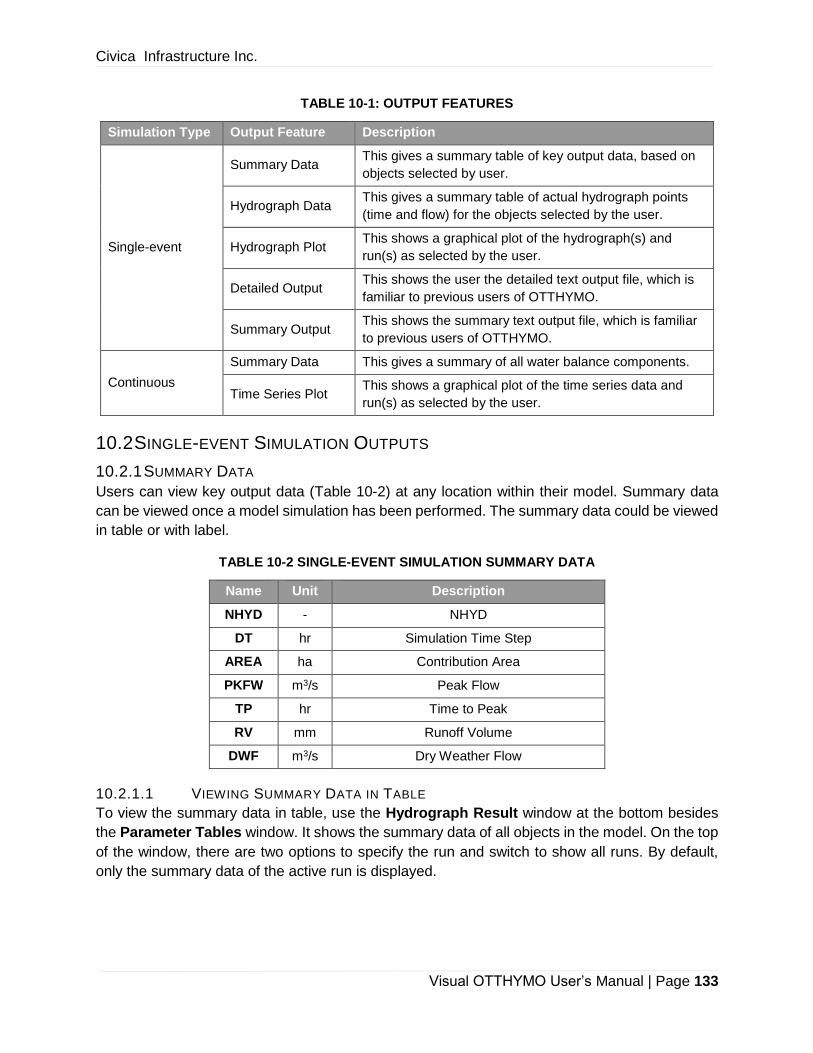
Civica Infrastructure Inc.
Visual OTTHYMO User’s Manual | Page 133
TABLE 10-1: OUTPUT FEATURES
Simulation Type Output Feature Description
Single-event
Summary Data This gives a summary table of key output data, based on
objects selected by user.
Hydrograph Data This gives a summary table of actual hydrograph points
(time and flow) for the objects selected by the user.
Hydrograph Plot This shows a graphical plot of the hydrograph(s) and
run(s) as selected by the user.
Detailed Output This shows the user the detailed text output file, which is
familiar to previous users of OTTHYMO.
Summary Output This shows the summary text output file, which is familiar
to previous users of OTTHYMO.
Continuous
Summary Data This gives a summary of all water balance components.
Time Series Plot This shows a graphical plot of the time series data and
run(s) as selected by the user.
10.2 SINGLE-EVENT SIMULATION OUTPUTS
10.2.1 SUMMARY DATA
Users can view key output data (Table 10-2) at any location within their model. Summary data
can be viewed once a model simulation has been performed. The summary data could be viewed
in table or with label.
TABLE 10-2 SINGLE-EVENT SIMULATION SUMMARY DATA
Name Unit Description
NHYD - NHYD
DT hr Simulation Time Step
AREA ha Contribution Area
PKFW m3/s Peak Flow
TP hr Time to Peak
RV mm Runoff Volume
DWF m3/s Dry Weather Flow
10.2.1.1 VIEWING SUMMARY DATA IN TABLE
To view the summary data in table, use the Hydrograph Result window at the bottom besides
the Parameter Tables window. It shows the summary data of all objects in the model. On the top
of the window, there are two options to specify the run and switch to show all runs. By default,
only the summary data of the active run is displayed.

Civica Infrastructure Inc.
Visual OTTHYMO User’s Manual | Page 134
When there are large number of objects, it’s necessary to only show the summary data of few
objects. To do this, first select the object on map view or schematic view and then click the Hy-
drograph Result button in Simulation tab. A new window is created besides the Map View
and Schematic View.
FIGURE 10-1 HYDROGRAPH RESULT
10.2.1.2 VIEWING SUMMARY DATA IN LABEL
VO can provide labels for each object on Schematic View, on an individual basis or all command
basis. The label content includes the NHYD, Name and hydrograph summary data. To create
labels:
1. Select the objects you wish to create a label for.
2. Right-click and select the Set Labels from the context menu to open the Label Editor
window (Figure 10-2), which lists all available label items.
3. Drag and drop the label items from Available Properties list on the left to Selected Prop-
erties list on the right.
4. Change the label background color with the color picker at the bottom.
5. Click OK to create the label.
6. To show the labels on canvas, select Show Labels from the context menu.
Note that the summary data value is empty if the output is not available.
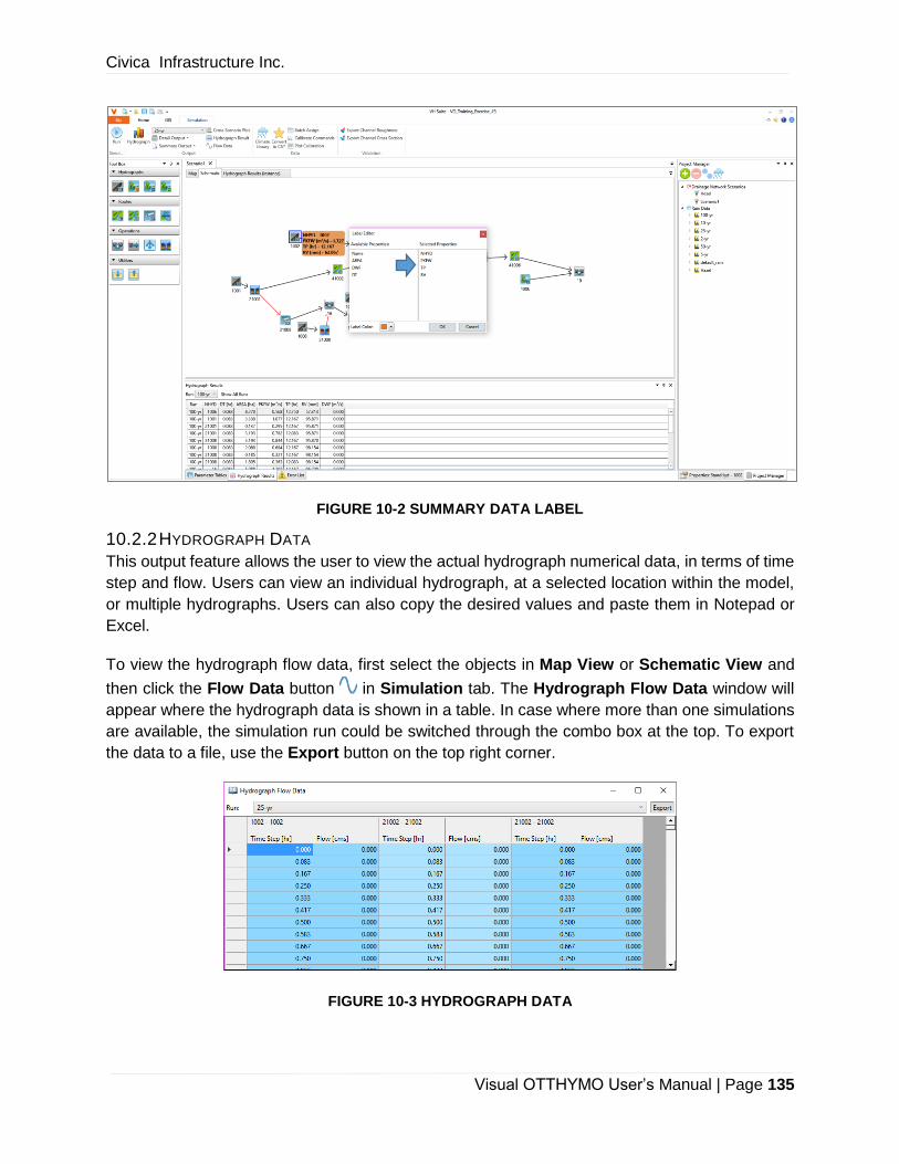
Civica Infrastructure Inc.
Visual OTTHYMO User’s Manual | Page 135
FIGURE 10-2 SUMMARY DATA LABEL
10.2.2 HYDROGRAPH DATA
This output feature allows the user to view the actual hydrograph numerical data, in terms of time
step and flow. Users can view an individual hydrograph, at a selected location within the model,
or multiple hydrographs. Users can also copy the desired values and paste them in Notepad or
Excel.
To view the hydrograph flow data, first select the objects in Map View or Schematic View and
then click the Flow Data button in Simulation tab. The Hydrograph Flow Data window will
appear where the hydrograph data is shown in a table. In case where more than one simulations
are available, the simulation run could be switched through the combo box at the top. To export
the data to a file, use the Export button on the top right corner.
FIGURE 10-3 HYDROGRAPH DATA
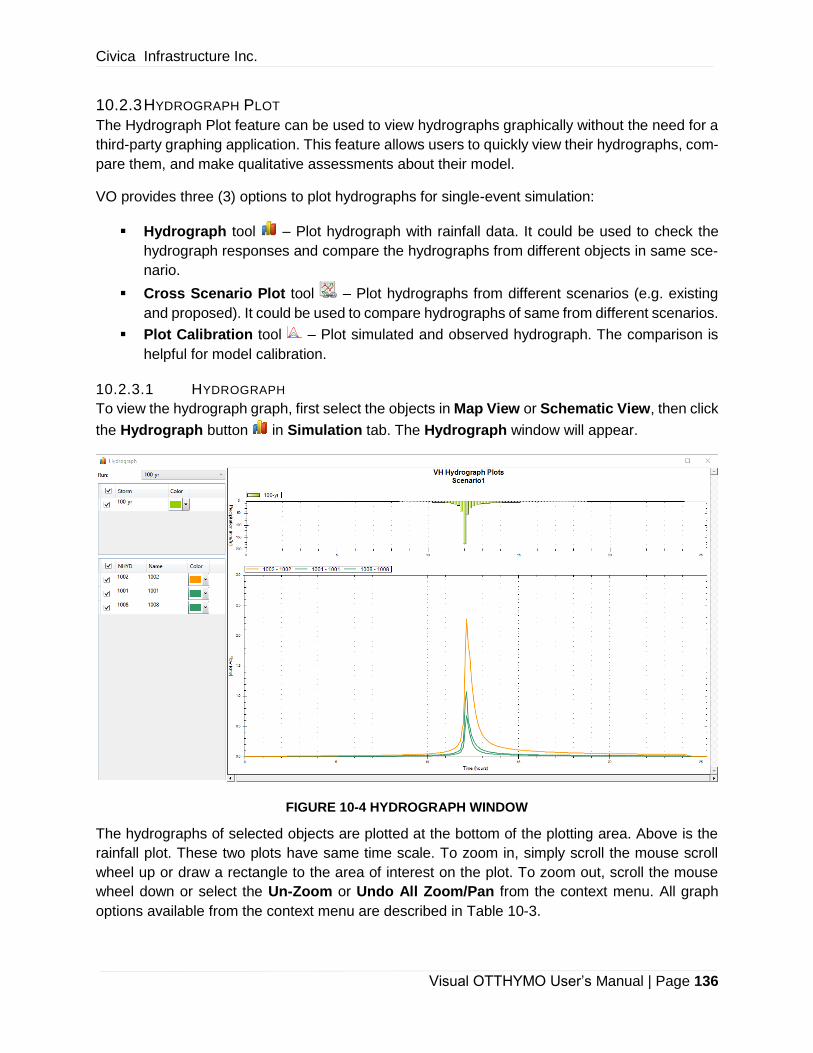
Civica Infrastructure Inc.
Visual OTTHYMO User’s Manual | Page 136
10.2.3 HYDROGRAPH PLOT
The Hydrograph Plot feature can be used to view hydrographs graphically without the need for a
third-party graphing application. This feature allows users to quickly view their hydrographs, com-
pare them, and make qualitative assessments about their model.
VO provides three (3) options to plot hydrographs for single-event simulation:
▪ Hydrograph tool – Plot hydrograph with rainfall data. It could be used to check the
hydrograph responses and compare the hydrographs from different objects in same sce-
nario.
▪ Cross Scenario Plot tool – Plot hydrographs from different scenarios (e.g. existing
and proposed). It could be used to compare hydrographs of same from different scenarios.
▪ Plot Calibration tool – Plot simulated and observed hydrograph. The comparison is
helpful for model calibration.
10.2.3.1 HYDROGRAPH
To view the hydrograph graph, first select the objects in Map View or Schematic View, then click
the Hydrograph button in Simulation tab. The Hydrograph window will appear.
FIGURE 10-4 HYDROGRAPH WINDOW
The hydrographs of selected objects are plotted at the bottom of the plotting area. Above is the
rainfall plot. These two plots have same time scale. To zoom in, simply scroll the mouse scroll
wheel up or draw a rectangle to the area of interest on the plot. To zoom out, scroll the mouse
wheel down or select the Un-Zoom or Undo All Zoom/Pan from the context menu. All graph
options available from the context menu are described in Table 10-3.

Civica Infrastructure Inc.
Visual OTTHYMO User’s Manual | Page 137
TABLE 10-3 GRAPH OPTIONS
Command Description
Copy Copies the graph
Save Image As… Saves the graphical image as the user-defined name
Page Setup… Allows user to modify the setup for the page
Print… Prints the hydrograph plot displayed
Show Point Values Graph will display the value that the cursor hovers
Un-Zoom Graph un-zooms the most recent zoom
Undo All Zoom/Pan Graph will return to its original scale
Panning Use the cursor to drag and pan the graph image
Zooming
Use the mouse scroll to zoom into and zoom out of the graph.
Enclose the specified area using the mouse to zoom into that
area.
The data source, visibility and color of the hydrographs could be changed with the controls on the
left side of the window. At the top is the simulation run selection box to switch to other simulation
runs. Below that are the controls for rainfall and hydrograph plots. Individual plots could be turned
off and changed to another color.
10.2.3.2 CROSS SCENARIO PLOT
The Cross Scenario Plot feature can be used to compare hydrographs from two different sce-
narios (e.g. existing and proposed) on the same graph. This is a good tool for quickly comparing
hydrographs at known locations, based on proposed modifications within the upstream catch-
ments.
To open the Cross Scenario Plot, click the Cross Scenario Plot button in the Simulation tab.
The Cross Scenario-Run Hydrograph Output window will appear (Figure 10-5). This window
has two parts with a tree view of all scenarios, simulations and objects on the left and the plot
area on the right.
No hydrograph is plotted when it’s first opened. To show the hydrographs, check the checkbox
on the left of the desired objects in the tree view. Although it’s possible to plot hydrographs of all
objects, it’s recommended to compare the hydrographs from the same objects.

Civica Infrastructure Inc.
Visual OTTHYMO User’s Manual | Page 138
FIGURE 10-5 CROSS SCENARIO PLOT WINDOW
10.2.3.3 PLOT CALIBRATION
It’s necessary to compare the observed and simulated hydrograph in model calibration. Plotting
the two hydrographs and the corresponding rainfall in the same plot is very helpful to guide the
calibration
Identifying the Gauge Objects
To compare to observed hydrograph, the location of the flow monitoring needs to be defined first.
This is done by selecting the object and then choosing Has Gauge Here from the context menu.
Importing Observed Data
To import the observed data and setup the comparison, click the Plot Calibration button . The
Compared to Observed Data window will appear. In this window, on the left is where the ob-
served data will be imported and the comparison could be configured on the right.

Civica Infrastructure Inc.
Visual OTTHYMO User’s Manual | Page 139
FIGURE 10-6 COMPARED TO OBSERVED DATA WINDOW
To add observed data, click the Add… button at the left bottom corner and select the observed
hydrograph data file. For file format, please refer to Chapter 11. The observed data will be added
to the Observed Data list. To remove it, select it in the list and click the Remove button at the
bottom.
Adding Result Comparison
There are three components in a result comparison: 1) observed data, 2) simulated data and 3)
corresponding rainfall. The observed data is added from the Observed Data list. The simulated
data is specified by selecting the simulation run and the corresponding hydrologic object. The
hydrograph from the specified object will be used to compare with the observed data. The corre-
sponding rainfall is the rainfall data that is responsible for the hydrograph response. It will be
plotted on the top of the hydrographs as a reference. It’s important to have this when analyzing
the observed and simulated hydrograph. If the observed hydrograph is not a clear response from
the rainfall, it may be necessary to check the rainfall data.
To create a result comparison, double-click an observed data in the Observed Data list or drag
it to the Comparison list on the right. A new result comparison will be added in the Comparison
list and the observed data is set to selected observed data. Once added, all the three components
could be changed by selecting desired items in the drop-down list. Note that Gauge Location
only lists the objects that has been set as a gauge using the Has Gauge Here context menu.
More than one comparison could be added using the same methods. This is useful for large
watersheds with multiple flow monitoring stations.
Viewing Observed and Simulated Plot
With results comparisons are created, it’s time to plot the observed and simulated hydrograph.
To view the plot, click the View button on the far-right side of each result comparison. The Ob-
served/Simulated Plot will appear (Figure 10-7).
The plot area is at the top where the rainfall is plotted above the observed and plotted hydrograph.
The observed hydrograph is in green and the simulated hydrograph is in red.

Civica Infrastructure Inc.
Visual OTTHYMO User’s Manual | Page 140
Below the plot area is the statistics of the two hydrographs including the minimum flow (m3/s),
maximum flow (m3/s), volume (m3) and relative difference of peak flow and volume. Often the
latter should be in an acceptable range for a calibrated model. For example, TRCA usually re-
quires the simulated volume should be +20% to -10% of the observed one and the simulated peak
flow should be +25% to -15% of the observed peak flow. The given relative difference in this
window would help determine if the simulated hydrograph is acceptable or not.
At the bottom is the control bar to navigate through multiple comparisons in cases where multiple
flow monitoring location are available. Click or to move the previous or next comparison
in the list. A summary information of current comparison is also shown between the two navigation
buttons.
FIGURE 10-7 OBSERVED/SIMULATED PLOT WINDOW
10.2.4 TRADITIONAL DETAILED AND SUMMARY OUTPUT
When a simulation is run successfully, VO generates traditional Summary Output and Detailed
Output and stores them in the project folder. For those new to OTTHYMO, the Summary Output
file is a text-based file that contains the key output data for each object during each storm simu-
lation. The Detailed Output file is a text-based file that contains all the output data for each object
during each storm simulation. Review agencies often require these text output files when review-
ing a model.

Civica Infrastructure Inc.
Visual OTTHYMO User’s Manual | Page 141
The detail output and summary output are available through the Detail Output button and
Summary Output button and their sub-menus in Simulation tab. The process to view and
export the detailed and summary output are similar. In this guide, only the detailed output is de-
scribed. You could easily follow the same steps for summary output.
Viewing Detailed Output
To view the detailed output of selected objects, first select the objects in Map View or Schematic
View, and then click the Detail Output button in Simulation tab. A new window will appear
besides the Schematic View tab. Note that the output of all simulation runs are listed. The infor-
mation in this view could be exported or copied to a file through the context menu.
FIGURE 10-8 DETAILED OUTPUT OF SELECTED OBJECTS (ALL SIMULATION RUNS)
To view the detailed output of all object in current simulation run, deselect all objects and click the
click the Detail Output button in Simulation tab. Similar to previous case, a new tab is created
besides the Schematic View to have all the information. To switch to another simulation run,
select it from the drop-down list above the Output button in Simulation tab.
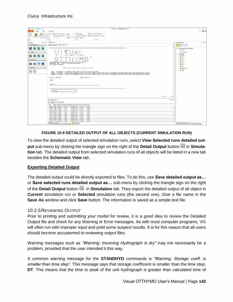
Civica Infrastructure Inc.
Visual OTTHYMO User’s Manual | Page 142
FIGURE 10-9 DETAILED OUTPUT OF ALL OBJECTS (CURRENT SIMULATION RUN)
To view the detailed output of selected simulation runs, select View Selected runs detailed out-
put sub-menu by clicking the triangle sign on the right of the Detail Output button in Simula-
tion tab. The detailed output from selected simulation runs of all objects will be listed in a new tab
besides the Schematic View tab.
Exporting Detailed Output
The detailed output could be directly exported to files. To do this, use Save detailed output as…
or Save selected runs detailed output as… sub-menu by clicking the triangle sign on the right
of the Detail Output button in Simulation tab. They export the detailed output of all object in
Current simulation run or Selected simulation runs (the second one). Give a file name in the
Save As window and click Save button. The information is saved as a simple text file.
10.2.5 REVIEWING OUTPUT
Prior to printing and submitting your model for review, it is a good idea to review the Detailed
Output file and check for any Warning or Error messages. As with most computer programs, VO
will often run with improper input and yield some suspect results. It is for this reason that all users
should become accustomed to reviewing output files.
Warning messages such as “Warning: Incoming Hydrograph is dry” may not necessarily be a
problem, provided that the user intended it this way.
A common warning message for the STANDHYD commands is “Warning: Storage coeff. is
smaller than time step”. This message says that storage coefficient is smaller than the time step,
DT. This means that the time to peak of the unit hydrograph is greater than calculated time of

Civica Infrastructure Inc.
Visual OTTHYMO User’s Manual | Page 143
concentration which could result in an underestimation of the peak flow. Therefore, the user
should reduce the DT to an integer value less than the storage coefficient. Do not reduce DT less
than 1.0. This warning message can be safely ignored when DT is set to 1.0.
All routing commands should be checked to ensure that the input rating curves have not been
exceeded, which will result in erroneous results.
10.3 CONTINUOUS SIMULATION OUTPUTS
There are two main difference between the output from continuous simulation and single-event
simulation.
1. The summary data is for the long-term time-series data including the water balance. Most
of the summary data is on average annual basis.
2. One hydrological object has multiple time series outputs.
10.3.1 SUMMARY DATA
The summary data in continuous simulation is listed in Table 10-4. Note that the average annual
summaries may not be the average annual values if the simulation time period doesn’t cover the
whole year.
TABLE 10-4 CONTINUOUS SIMULATION SUMMARY DATA
Name Unit Description
NHYD - NHYD
P mm Average Annual Precipitation
Rain mm Average Annual Rainfall
Snow mm Average Annual Snowfall
Snowmelt mm Average Annual Snowmelt
ET mm Average Annual Evapotranspiration
INFIL mm Average Annual Infiltration
GWI mm Average Annual Groundwater Infiltration
Runoff mm Average Annual Runoff
Runoff Coef - Average Annual Runoff Coefficient
Peak Flow m3/s Peak Flow
Peak Flow Time - The Time when Peak Flow Happens
Similar with single-event simulation, the summary data could be viewed in table or with label as
shown in Figure 10-10. For continuous simulation, the summary data window is changed to Water
Balance Result. Note that the water balance summary data is only available for catchments (i.e.
NasHyd and StandHyd).

Civica Infrastructure Inc.
Visual OTTHYMO User’s Manual | Page 144
FIGURE 10-10 CONTINUOUS SIMULATION SUMMARY DATA IN TABLE AND LABEL
The water balance could also be summarized on monthly and yearly basis. To view the monthly
and yearly water balance summary, choose the Water Balance menu from Schematic View con-
text menu. The Water Balance window will appear (Figure 10-11).
On the left is the yearly and monthly water balance summary table shown in two tabs. Besides
the summary data of each year and month, the average is also given at the bottom. For month
summary, a total summary is also available which basically is the average annual summary.
On the right side is a pie chart to highlight the three important water balance components: Infiltra-
tion, ET and Runoff. The chart is corresponding to the active summary data row in the summary
table. To change to another summary data, click on the desired row or use the arrow key to move
up and down. In this pie chart, default colors are used: green for ET, red for runoff and blue for
infiltration. Note that the percentage in the pie chart is the percentage of the total of the three
components. For runoff, it’s not the runoff coefficient.
The water balance summary table could be for individual catchment or for all catchments. To
show the summary table for individual catchment, select it before choosing the Water Balance
context menu. For all catchments, deselect all objects before choosing the Water Balance con-
text menu.

Civica Infrastructure Inc.
Visual OTTHYMO User’s Manual | Page 145
FIGURE 10-11 WATER BALANCE WINDOW
10.3.2 TIME SERIES PLOT
Multiple time series data are available for each hydrologic object. The available time series is
different depending on the type of the objects. The time series could be viewed using three tools:
1. Hydrograph - Plot the simulated flow data with precipitation data.
2. Plot Results - Plot selected time series data with given time interval.
3. Plot Calibration - Plot observed and simulated flow or water level.
10.3.2.1 HYDROGRAPH
Flow data is available from all hydrologic objects. To view the flow data, select the objects in Map
View or Schematic View, and then click the Hydrograph button in Simulation tab. The Hy-
drograph window will appear (Figure 10-12). This window is same as the single-event hydrograph
window. For more information, please see 10.2.3.1.

Civica Infrastructure Inc.
Visual OTTHYMO User’s Manual | Page 146
FIGURE 10-12 CONTINUOUS SIMULATION HYDROGRAPH WINDOW
10.3.2.2 PLOT RESULTS
To view other time series data, select the objects in Map View or Schematic View, and then click
the Plot Results button in Simulation tab. The Plot Results window will appear.
On the left side is the control panel to control the data source and appearance of the plots. From
the top to bottom, the options are:
1. Run – The simulation run.
2. Type – The type of objects. Objects of same type have similar time series.
3. Variables – The available time series.
4. Interval – The time interval the time series data will be summarized and displayed. The
options are Original, Day, Week, Month and Year. The original will use the simulation time
step. The line graph is used for Original, day and week. Month and Year will use the bar
chart.
Below the control panel is the list of selected objects where the plot visibility and color could be
changed. As continuous simulation tends to have large amount data in each time series data, it’s
not recommended to display many objects at the same time.
An example is shown in Figure 10-13. In the first screenshot, the flow is plotted with 5-min time
interval. The same time series is summarized on week basis and plotted in the second screen-
shot.
The time series data could be exported to a simple CSV file by clicking the Export button on
the top left corner.

Civica Infrastructure Inc.
Visual OTTHYMO User’s Manual | Page 147
FIGURE 10-13 CONTINUOUS SIMULATION PLOT RESULTS WINDOW
10.3.2.3 PLOT CALIBRATION
Similar to single-event simulation, it’s important to compare the observed and simulated time-
series data for model calibration. As there are more than one time-series data is available, it’s
necessary to specify the one used for the comparison. This is done by selecting the Observed
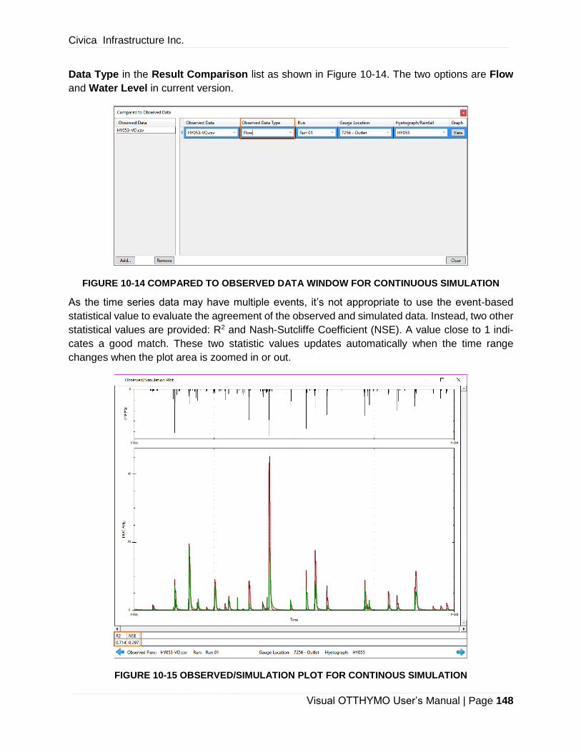
Civica Infrastructure Inc.
Visual OTTHYMO User’s Manual | Page 148
Data Type in the Result Comparison list as shown in Figure 10-14. The two options are Flow
and Water Level in current version.
FIGURE 10-14 COMPARED TO OBSERVED DATA WINDOW FOR CONTINUOUS SIMULATION
As the time series data may have multiple events, it’s not appropriate to use the event-based
statistical value to evaluate the agreement of the observed and simulated data. Instead, two other
statistical values are provided: R2 and Nash-Sutcliffe Coefficient (NSE). A value close to 1 indi-
cates a good match. These two statistic values updates automatically when the time range
changes when the plot area is zoomed in or out.
FIGURE 10-15 OBSERVED/SIMULATION PLOT FOR CONTINOUS SIMULATION
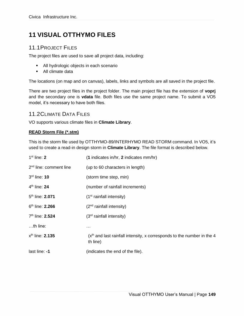
Civica Infrastructure Inc.
Visual OTTHYMO User’s Manual | Page 149
11 VISUAL OTTHYMO FILES
11.1 PROJECT FILES
The project files are used to save all project data, including:
▪ All hydrologic objects in each scenario
▪ All climate data
The locations (on map and on canvas), labels, links and symbols are all saved in the project file.
There are two project files in the project folder. The main project file has the extension of voprj
and the secondary one is vdata file. Both files use the same project name. To submit a VO5
model, it’s necessary to have both files.
11.2 CLIMATE DATA FILES
VO supports various climate files in Climate Library.
READ Storm File (*.stm)
This is the storm file used by OTTHYMO-89/INTERHYMO READ STORM command. In VO5, it’s
used to create a read-in design storm in Climate Library. The file format is described below.
1st line: 2 (1 indicates in/hr, 2 indicates mm/hr)
2nd line: comment line (up to 60 characters in length)
3rd line: 10 (storm time step, min)
4th line: 24 (number of rainfall increments)
5th line: 2.071 (1st rainfall intensity)
6th line: 2.266 (2nd rainfall intensity)
7th line: 2.524 (3rd rainfall intensity)
…th line: …
xth line: 2.135 (xth and last rainfall intensity, x corresponds to the number in the 4
th line)
last line: -1 (indicates the end of the file).
Civica Infrastructure Inc.
Visual OTTHYMO User’s Manual | Page 150
An example of a Storm data file (25mm4hr.stm) is as follows:
2
TWENTY-FIVE MM FOUR HOUR CHICAGO STORM
10
24
2.071
2.266
2.524
2.880
3.382
4.175
5.696
10.777
50.214
13.366
8.286
6.295
5.194
4.466
3.949
3.560
3.252
3.010
2.799
2.622
2.476
2.346
2.233
2.136
-1
MASS STORM File (*.mst)
This is the storm file used by OTTHYMO-89/INTERHYMO MASS STORM command. In VO5, it’s
used to create a MASS storm in Climate Library. The file format is described below. Note that
the ordinate is the fraction of the accumulated rainfall volume to total volume. So it starts from 0
and increases to 1.
1st line: comment line (up to 60 characters in length)
2nd line: 20 (the time increment between each ordinate, min)
3rd line: 13 (the # of ordinates used to describe the mass curve, max.=400)

Civica Infrastructure Inc.
Visual OTTHYMO User’s Manual | Page 151
4th line: 0.00 (the first ordinate of the mass curve)
5th line: 0.01 (the second ordinate of the mass curve)
6th line: 0.04 (the third ordinate of the mass curve)
…th line: …
xth line: 1.00 (xth and last ordinate of the mass curve)
last line: -1 (indicates the end of the file).
An example of a MASS Storm data file (aesmass.mst) is as follows:
AES MASS CURVE DATA WITH TWENTY MINUTE TIME STEP
20
13
0.00
0.01
0.04
0.12
0.27
0.55
0.70
0.82
0.90
0.95
0.98
0.99
1.00
-1
Simple CSV
The simple CSV files are used to import the precipitation, temperature and evaporation data. Two
columns are required for precipitation and evaporation. The daily temperature file has three col-
umns with date time, minimum daily temperature and maximum daily temperature.
11.3 CALIBRATION FILES
The calibration files are used to import the observed time series data and compare to the simula-
tion outputs. Two file formats are supported: 1) SWMM format and 2) simple CSV format.
SWMM Format
The SWMM calibration file format is supported. From SWMM user’s manual, the format of the file
is as follows:

Civica Infrastructure Inc.
Visual OTTHYMO User’s Manual | Page 152
1. The name of the first object with calibration data is entered on a single line. This name will
be the observation data name in Plot Calibration tool.
2. Subsequent lines contain the following recorded measurements for the object:
▪ Measurement date (month/day/year, e.g. 6/21/2004). Note that the elapsed time
format is not supported.
▪ Measurement time (hours:minutes) on the measurement date or relative to the
number of elapsed days
▪ Measurement values
3. Follow the same sequence for any additional objects.
An excerpt from an example file is shown below. It contains flow at two locations FG02HC023
and FG02HC009. Note that a semicolon can be used to begin a comment.
Simple CSV Format
The simple CSV format has two columns: 1) measurement date and time column and 2) meas-
urement value. It’s assumed that the first row is the header and will be ignored.
11.4 HYDROGRAPH FILES
If the READ HYD object is used to read an external hydrograph file into the model, then the file
must be coded in the correct format. This format is in the same format as the hydrograph files
used in OTTHYMO-89/ITNERHYMO. Therefore, previously made hydrograph files (from SAVE
HYD command) may be used. The file format is described below.
1st line: 2 (1 indicates in/hr, 2 indicates mm/hr)
2nd line: comment line (up to 60 characters in length)
3rd line: 5 (storm time step, min)

Civica Infrastructure Inc.
Visual OTTHYMO User’s Manual | Page 153
4th line: 50 (the catchment area from which the hydrograph was obtained, ha or
acre)
5th line: 0.000 (1st hydrograph ordinate, m3/s or cfs)
6th line: 0.100 (2nd hydrograph ordinate, m3/s or cfs)
7th line: 0.200 (3rd hydrograph ordinate, m3/s or cfs)
…th line: …
xth line: 0.100 (xth and last hydrograph ordinate)
last line: -1 (indicates the end of the file).
An example of a Hydrograph data file (test.hyd) is as follows:
2
HYDROGRAPH FROM OUR TEST CATCHMENT
5
50
0
0.000
0.100
0.200
0.300
1.000
1.200
4.500
8.150
10.000
9.500
5.450
2.000
1.000
0.500
0.300
0.100
-1

Civica Infrastructure Inc.
Visual OTTHYMO User’s Manual | Page 154
12 TROUBLESHOOTING
This Chapter has been written to aid users in resolving some of the more simple problems, warn-
ing messages, and error messages that might arise when using the model. These problems or
messages may be attributed to invalid input, using the model for situations where it was not de-
signed to be used, or not following a procedure properly as set out in the User’s Manual.
12.1 ERROR AND WARNING MESSAGES
Error and warning messages can appear within the interface and within the Detailed Output
Files. The messages stem from an input error or computational error, which is likely caused by
the input variables. This section outlines the more common messages and gives a brief descrip-
tion of their meaning.
12.1.1 INTERFACE FILE MESSAGES
Unable to save project: Project files can only be saved on a drive with a capacity of 10MB or
more (e.g. local hard-drive or network drive). It is recommended that you only run models from
local or network hard drives.
Multi-Instance is not allowed: You can only run one copy of VO on your machine at a time.
You have exceeded the maximum number of objects for this license,: The version of VO you
are running has a specific number of objects allowed, per project. This number has been ex-
ceeded. Either decrease the number of objects or upgrade your version.
12.1.2 OUTPUT FILE MESSAGES
ERROR: CHECK NUMBER OF RAINFALL INCREMENTS: This occurs in the old URBHYD com-
mand where the number of rainfall increments was an input variable. It therefore has to match
with the storm being simulated.
ERROR: CHECK THE STORAGE-DISCHARGE TABLE.: There is an error in the input variables
in the storage-discharge table.
ERROR: UNITS OF INPUT DATA NOT SPECIFIED: Either the scenario or project settings have
a conflict in the input units. Make sure the each is consistent (i.e. metric or imperial).
ERROR: SHIFT TO LARGE, RAIN ELIMINATED.: This error occurs with the SHIFT HYD com-
mand. If the shift is too large the rainfall may be eliminated past the 800 point time steps.
ERROR: TIME STEP = 0, COMMAND ABORTED.: A DT of 0 has been input and is unaccepta-
ble.
ERROR: RAINFALL INCREMENT = 0, COMMAND ABORTED.: The number of rainfall incre-
ments is zero, therefore runoff will not be calculated.
Civica Infrastructure Inc.
Visual OTTHYMO User’s Manual | Page 155
WARNING: A MINIMUM SURCHARGE OF (X) CAN BE EXPECTED WITH THE GIVEN PIPE.:
This is from the ROUTE PIPE command. The message indicates surcharge may occur due to
lack of conveyance capacity.
WARNING: AVERAGE OF EFFECTIVE RAINFALL INTENSITIES AS MADE (X) OVER A TIME
LARGER THAN THE DURATION OF THE STORM: Try reducing the DT of the hydrograph.
WARNING: CANNOT COMPUTE 1a WHEN USING PROPORTIONAL LOSS METHOD: The
initial abstraction cannot be calculated (i.e. cannot be -1) when using the proportional loss
method. It must be specified by the user.
WARNING: COMPUTATIONS FAILED TO CONVERGE.: The routing time step is too large, try
reducing it.
WARNING: FIRST OUTFLOW IS NOT ZERO.: The first point in a ROUTE RESERVOIR com-
mand must be 0,0.
WARNING: FOR AREAS WITH IMPERVIOUS RATIOS BELOW 20%, YOU SHOULD CON-
SIDER SPLITTING THE AREA.: This is a warning for STANDHYD. The STANDHYD command
was designed for areas with impervious ratios greater than or equal to 20%. When the ratio is
less than this value, the runoff may not be correct. The catchment should therefore be split into
impervious and pervious components.
WARNING: HYDROGRAPH PEAK WAS NOT REDUCED. CHECK OUTFLOW/ STORAGE TA-
BLE OR REDUCE DT.: The routing command did not reduce the peak flow. Reduce the DT,
check the input variables, or review the assumptions made with routing object.
WARNING: HYDROGRAPH WAS CUT. CHECK VOLUME.: This happens in routing commands
and may be cause by too large of a DT or too many points in the hydrograph (i.e. approaching
800). If the volume out is only marginally less than the volume in, then this may not be of concern.
WARNING: LENGTH OF STORM HAD TO BE CUT FROM (X) POINTS TO 800.: The maximum
number of hyetograph points is 800. The rest have been truncated. To include all points increase
the DT of the storm file and hydrographs computations as well.
WARNING: MINIMUM PIPE SIZE REQUIRED = (X) FOR FREE FLOW. THIS SIZE WAS USED
IN THE ROUTING.: Too small of a pipe size was input. The program automatically calculated a
new size and this was used in the routing calculations.
WARNING: N DID NOT CONVERGE AFTER 50 ITERATIONS.: This is from the WILHYD com-
mand. There was a problem calculating an internal number for the number of linear reservoirs.
Check the input parameters and re-run.
WARNING: SELECTED ROUTING TIME STEP DENIED.: The DT of the routing command is not
less than or equal to the DT of the incoming hydrograph. Change the input parameter for this
command.

Civica Infrastructure Inc.
Visual OTTHYMO User’s Manual | Page 156
WARNING: SLOPE <=0.0 (HYD WAS ONLY TRANSFERRED): This is from the ROUTE PIPE
Command. The pipe slope must be positive or there is no routing calculated.
WARNING: STORAGE COEFF. IS SMALLER THAN TIME STEP!: The peak flow may be un-
derestimated since the storage coefficient relates to the time-to-peak of the unit hydrograph. Us-
ers should manually decrease the DT of the hydrograph until the warning disappears or the DT is
as small as 1.0 minute.
WARNING: THE PERVIOUS AREA HAS NO FLOW.: This may happen for small storms where
the runoff volume is low, or in cases where the catchment imperviousness is high. Check the LGP
parameter as well. It could be too high.
WARNING: THE TABLE WAS EXTRAPOLATED FROM (X) TO THE END.: The rating curve
table has been extrapolated. Add more points to the rating curve.
WARNING: TRAVEL TIME TABLE EXCEEDED.: For a ROUTE CHANNEL command, the rating
curve table has been exceeded. Add more points to the channel geometry. Also this could result
from too large of a computation time step.
12.2 PROGRAM QUITS DURING RUN SIMULATION
The most common cause of the program quitting during a run simulation is due to incorrect input.
To isolate the suspect input, try the following:
1. After the program quits, open the Detailed Output file using a text editor. Make note of the
command (by NHYD) where the simulation appears to have stopped.
2. If there are Warning or Error messages refer to the previous section in this Manual for an
explanation on the message.
3. Re-open the Project and suspect scenario and view the parameters of the object in
question. Make any adjustments as required. If the scenario will not open then retrieve a
backup copy from the BACKUP folder located in the project folder.
4. If the object parameters are acceptable then the error could be from the rainfall
information. If using an external rainfall file, confirm that it is present and that the format is
correct (refer to Reference Manual for format). To see whether the rainfall file is where the
error occurs, try running the scenario with the default Chicago Storm.
5. Failing the above, try importing the scenario into a new project with only one scenario
contained in the project.
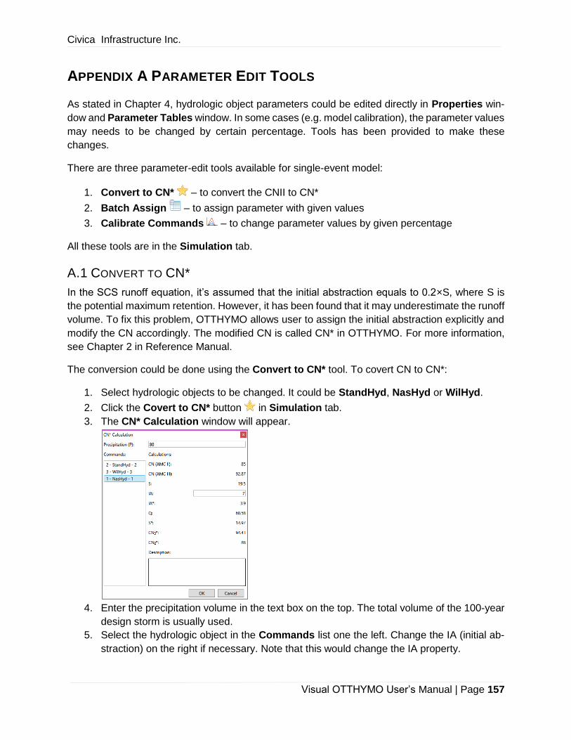
Civica Infrastructure Inc.
Visual OTTHYMO User’s Manual | Page 157
APPENDIX A PARAMETER EDIT TOOLS
As stated in Chapter 4, hydrologic object parameters could be edited directly in Properties win-
dow and Parameter Tables window. In some cases (e.g. model calibration), the parameter values
may needs to be changed by certain percentage. Tools has been provided to make these
changes.
There are three parameter-edit tools available for single-event model:
1. Convert to CN* – to convert the CNII to CN*
2. Batch Assign – to assign parameter with given values
3. Calibrate Commands – to change parameter values by given percentage
All these tools are in the Simulation tab.
A.1 CONVERT TO CN*
In the SCS runoff equation, it’s assumed that the initial abstraction equals to 0.2×S, where S is
the potential maximum retention. However, it has been found that it may underestimate the runoff
volume. To fix this problem, OTTHYMO allows user to assign the initial abstraction explicitly and
modify the CN accordingly. The modified CN is called CN* in OTTHYMO. For more information,
see Chapter 2 in Reference Manual.
The conversion could be done using the Convert to CN* tool. To covert CN to CN*:
1. Select hydrologic objects to be changed. It could be StandHyd, NasHyd or WilHyd.
2. Click the Covert to CN* button in Simulation tab.
3. The CN* Calculation window will appear.
4. Enter the precipitation volume in the text box on the top. The total volume of the 100-year
design storm is usually used.
5. Select the hydrologic object in the Commands list one the left. Change the IA (initial ab-
straction) on the right if necessary. Note that this would change the IA property.
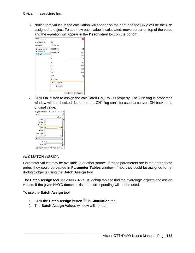
Civica Infrastructure Inc.
Visual OTTHYMO User’s Manual | Page 158
6. Notice that values in the calculation will appear on the right and the CN2* will be the CN*
assigned to object. To see how each value is calculated, move cursor on top of the value
and the equation will appear in the Description box on the bottom.
7. Click OK button to assign the calculated CN2* to CN property. The CN* flag in properties
window will be checked. Note that the CN* flag can’t be used to convert CN back to its
original value.
A.2 BATCH ASSIGN
Parameter values may be available in another source. If these parameters are in the appropriate
order, they could be pasted in Parameter Tables window. If not, they could be assigned to hy-
drologic objects using the Batch Assign tool.
The Batch Assign tool use a NHYD-Value lookup table to find the hydrologic objects and assign
values. If the given NHYD doesn’t exist, the corresponding will not be used.
To use the Batch Assign tool:
1. Click the Batch Assign button in Simulation tab.
2. The Batch Assign Values window will appear.

Civica Infrastructure Inc.
Visual OTTHYMO User’s Manual | Page 159
3. Check the property to be changed on the left panel. The properties are listed based on
object type.
4. Copy the data from the source and past in the table on the right. The data should have
two columns. The first column could be NHYD or NAME, which will be used to search
hydrologic object by NHYD and NAME. To use NAME, check the Select command by
name instead of NHYD above the table. The second column is the parameter value to
assigned. In the example given below, the CN of NasHyd will be updated. And the
NasHyd with NHYD of 1 will be searched. If successful, its CN value will be assigned to
80.
5. Click Assign button on the right bottom corner to assign the values.
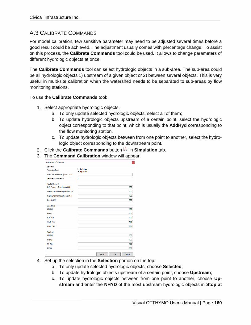
Civica Infrastructure Inc.
Visual OTTHYMO User’s Manual | Page 160
A.3 CALIBRATE COMMANDS
For model calibration, few sensitive parameter may need to be adjusted several times before a
good result could be achieved. The adjustment usually comes with percentage change. To assist
on this process, the Calibrate Commands tool could be used. It allows to change parameters of
different hydrologic objects at once.
The Calibrate Commands tool can select hydrologic objects in a sub-area. The sub-area could
be all hydrologic objects 1) upstream of a given object or 2) between several objects. This is very
useful in multi-site calibration when the watershed needs to be separated to sub-areas by flow
monitoring stations.
To use the Calibrate Commands tool:
1. Select appropriate hydrologic objects.
a. To only update selected hydrologic objects, select all of them;
b. To update hydrologic objects upstream of a certain point, select the hydrologic
object corresponding to that point, which is usually the AddHyd corresponding to
the flow monitoring station.
c. To update hydrologic objects between from one point to another, select the hydro-
logic object corresponding to the downstream point.
2. Click the Calibrate Commands button in Simulation tab.
3. The Command Calibration window will appear.
4. Set up the selection in the Selection portion on the top.
a. To only update selected hydrologic objects, choose Selected;
b. To update hydrologic objects upstream of a certain point, choose Upstream;
c. To update hydrologic objects between from one point to another, choose Up-
stream and enter the NHYD of the most upstream hydrologic objects in Stop at

Civica Infrastructure Inc.
Visual OTTHYMO User’s Manual | Page 161
Commands (Exclusive) text box. Multiple NHYDs should be separated by
comma.
For the model given below, the AddHyd 5 is selected. The updated hydrologic objects
with the three options are given below.
a. Only AddHyd 5 will be updated if Selected is used;
b. NasHyd 1&2, RouteChannel 3&4 and AddHyd 5 will be updated if Upstream is
used.
c. RouteChannel 3&4 and AddHyd 5 will be updated if Upstream is used and Stop
at Commands (Exclusive) is set to 3,4.
The number of updated hydrologic objects will be given at Selected Commands in Se-
lection section. Note it’s not always the number of selected hydrologic objects.
5. Specify the percentage change for RouteChannel, StandHyd and NasHyd in the three
sections below the Selection section. All common parameters are listed and the default
value is 100. To decrease the parameter values, enter a value smaller than 100 (e.g. 80).
Otherwise, enter a value larger than 100 (e.g. 120).
6. Click OK button to apply the changes.


