This article was downloaded by: [UZH Hauptbibliothek / Zentralbibliothek Zürich]On: 10 July 2014, At: 10:28Publisher: Taylor & FrancisInforma Ltd Registered in England and Wales Registered Number: 1072954 Registered office: Mortimer House,37-41 Mortimer Street, London W1T 3JH, UK

Optimization: A Journal of Mathematical Programmingand Operations ResearchPublication details, including instructions for authors and subscription information:http://www.tandfonline.com/loi/gopt20

Vector approximation problems in geometric vectoroptimizationK. H. Elster a & R. Elster ba Institute of Mathematics , University of Verona , via delVArtigliere 19, Verona, 37129,ItalyOn leave from the Technische Universität Ilmenau ,Germanyb Institute of Statistics and Mathematical Economics , university of Karlsruhe , P.O. Box6980, W-7500Karlsruhe, GermanyPublished online: 18 May 2010.

To cite this article: K. H. Elster & R. Elster (1993) Vector approximation problems in geometric vectoroptimization, Optimization: A Journal of Mathematical Programming and Operations Research, 27:4, 321-342, DOI:10.1080/02331939308843893

To link to this article: http://dx.doi.org/10.1080/02331939308843893

PLEASE SCROLL DOWN FOR ARTICLE

Taylor & Francis makes every effort to ensure the accuracy of all the information (the “Content”) containedin the publications on our platform. However, Taylor & Francis, our agents, and our licensors make norepresentations or warranties whatsoever as to the accuracy, completeness, or suitability for any purpose of theContent. Any opinions and views expressed in this publication are the opinions and views of the authors, andare not the views of or endorsed by Taylor & Francis. The accuracy of the Content should not be relied upon andshould be independently verified with primary sources of information. Taylor and Francis shall not be liable forany losses, actions, claims, proceedings, demands, costs, expenses, damages, and other liabilities whatsoeveror howsoever caused arising directly or indirectly in connection with, in relation to or arising out of the use ofthe Content.

This article may be used for research, teaching, and private study purposes. Any substantial or systematicreproduction, redistribution, reselling, loan, sub-licensing, systematic supply, or distribution in anyform to anyone is expressly forbidden. Terms & Conditions of access and use can be found at http://www.tandfonline.com/page/terms-and-conditions

Optimization, 1993, Vol. 27, pp. 321-342 0 1993 Gordon and Breach Science Publishers S.A. Reprints available directly from the publisher Printed in the United States of America Photocopying permitted by license only

VECTOR APPROXIMATION PROBLEMS IN GEOMETRIC VECTOR OPTIMIZATION

K.-H. ELSTERT and R. ELSTER*

.i. University of Verona, Institute of Mathematics, via dell'Artigliere 19, 37129 Verona, Italy. On leave from the Technische Universitat Ilmenau, Germany. $ University of Karlsruhe, Institute of Statistics and Mathematical Economics,

P. 0. Box 6980, W-7500 Karlsruhe, Germany.

(Received 27 April 1992; in final form 20 October 1992)

Using the geometric vector inequality, introduced by Elster/Elster/Gopfert [9], we consider a special case of that inequality which is a basis for treating certain classes of (nonsmooth) vector optimization problems: vector curve fitting problems, (,-vector approximation problems and vector regression problems. By the introduced geometric vector inequality we obtain in a natural way dual problems for such special-structured vector optimization problems, which can be solved in an efficient manner, since the dual constraints are linear.

KEY WORDS Vector optimization, vector approximation problems, duality, geometric vector inequality, Legendre vector transform.

Mathematics Subject Classification 1991: Primary: 90C29; Secondary: 90C28

1. INTRODUCTION

In the present paper the geometric vector inequality, introduced in 191, will be used for a systematic investigation of special structured vector optimization problems. Especially, certain nonsmooth vector optimization problems are treated with the aid of smooth problems. It turns out that a special geometric vector inequality can be considered as a basis to establish classes of problems of considerable interest, such as vector curve fitting problems, tp-vector approxima- tion problems, and vector regression problems.

For that purpose we treat in Section 2 properties of the Legendre vector transform and a vector norm. This section contains further the main result concerning the above mentioned geometric vector inequality, which leads straight to geometric vector optimization problems (Section 3). Moreover, dual problems can be introduced, where the dual feasible set is exclusively represented by linear constraints. This may be an advantage from the numerical viewpoint.

Some earlier results concerning geometric vector inequalities are given in [s, 6,71.

2. NOTATIONS

We denote by R the set of reals, by R + the set of nonnegative real numbers, by R t the set of positive real numbers and by R" the n-dimensional Euclidean

321

Dow

nloa

ded

by [

UZ

H H

aupt

bibl

ioth

ek /

Zen

tral

bibl

ioth

ek Z

üric

h] a

t 10:

28 1

0 Ju

ly 2

014

322 K.-H. ELSTER AND R. ELSTER

space. Let be given the index sets

J:+~:= (0, 1 , . . . , S , s + 1, . . . , s + p ) , (la) J O := J:+,\ J:, ( lb)

[k] := {mk, mk + 1, . . . , nk), k E J:+,, l[k]l= card[k], PC)

wherem,:=l , m l : = n , + l , . . . , m , + p : = n , + p ~ l + l , n,+,:=n. Moreover, let

s +P c Rl[kll, k E Jy+p, open convex sets, S := x Sk G Rn; Sk -

k=O (4

Tk c R'[kl', k E J:+p, nonempty cones with the vertex (3) at the origin, T := x$L~O Tk G Rn;

G; : Sk + R, k E J:+p, differentiable functions, (4a)

We introduce the matrices

("evaluation matrix" of the decision maker, ((.(I Euclidean norm);

Ez := (E' 1 ZE2), El , E' identity matrices (7) in [w(s+l)x(s+~) and in RPxP, respectively;

where

r1 := (6 - . 1) =

(8b)

r2 := . ) = diag(yk)klJ, yk c R+ Vk; Ys +p

where

Dow

nloa

ded

by [

UZ

H H

aupt

bibl

ioth

ek /

Zen

tral

bibl

ioth

ek Z

üric

h] a

t 10:

28 1

0 Ju

ly 2

014

VECTOR APPROXIMATION PROBLEMS 323

and A, : T -, R +, k E J:+,, arbitrary (nonnegative) functions

such that ( 9 ~ )

A ) := ( [ k l ) ) where A; : T,+ R +; ( 9 4

By the matrices introduced above we obtain

3. THE GEOMETRIC VECTOR INEQUALITY AND THE LEGENDRE VECTOR TRANSFORM

Using the notations given above we are going to introduce the geometric vector inequality as a generalization of the well-known geometric inequality which was used by Duffin/Peterson/Zener [3] for developing the geometric optimization as an interesting area in (scalar) nonlinear optimization, important both in theory and applications.

Definition 1: The vector inequality

is called geometric vector inequality, if

= diag(d,k](~)~)k,J:+~

with 0 f dlk1(x) E Tk V k E J,O+p, such that

Yzx = Az(y)G(x) - EZV(Y)

VY = . . . , Y ~ + ~ ~ ~ ~ + ~ ~ ( x ) ~ ) ~ E T, yk E R + Vk E JS+~. Then

YZ = EzY VY = T D = d iag (ykd ,k , (~ )T)ksJ : l , p .

For any geometric vector inequality the following "translation property" is satisfied. D

ownl

oade

d by

[U

ZH

Hau

ptbi

blio

thek

/ Z

entr

albi

blio

thek

Zür

ich]

at 1

0:28

10

July

201

4

324 K.-H. ELSTER AND R. ELSTER

Theorem 1: Let the geometric vector inequality (13) be given. If C E R n is fixed, then for any a E RS+'+p the inequality

YZX SAz(y)[G(x + C) + a ] - [EzV(Y) + YzC +Az(y)aI X E S ' : = S - C , Y E T

(14)

is a geometric vector inequality, too.

Proof: By the assumptions we have for arbitrary x' E S, y E T the vector inequality

YZxl I AZ(y)G(x1) - EzV(y).

Thus we obtain for x := x' - C

and hence for each x E S' and each y E T

Since S' is an open convex set, obtained by translation of S, and since the cone T is invariant with respect to the translation x = x ' - C, the matrix D which exists according Definition 1 for each x E St , satisfies not only (13) but also (14) as an equality. .

For the treatment of certain vector optimization problems we use a special geometric vector inequality in which the main diagonal vector of the matrix A(y) (cf. (12b)) is the so-called Legendre vector transform, and in which the function G is a vector norm. The vector norm considered in the following is a modification of that given by Jahn [14], Jahn/Krabs [15], Bacopoulos/Godini/ Singer [I], [2], Gearhart [ l l ] .

Definition 2: Let F : S -, Rs+l+p be an iW",+'-convex? vector function according to (4b), let S be given according to (2). Furthermore, let

Wz = EzW = EzJF(r) (15a) where

is the "diagonalized Jacobian". Then the vector function [L' : L,, -t R S f 1 (L,, is the vectorspace of the (s + 1) x n matrices), where

is called Legendre vector transform of F. Now we introduce the vector norm.

t F : S + R"+'+P, S according to (2), is said to be R?'-convex, if for x' , x Z E S and any a E [ O , 11 holds E , ( ~ F ( x ' ) + (1 - ~ ) F ( x ~ ) - F ( ~ x ' + (1 - m)x2)] E rwyl. D

ownl

oade

d by

[U

ZH

Hau

ptbi

blio

thek

/ Z

entr

albi

blio

thek

Zür

ich]

at 1

0:28

10

July

201

4

VECTOR APPROXIMATION PROBLEMS 325

Definition 3: A map III.III : Rn+ Rq is called a vector norm, if the following properties are satisfied:

Using these notations the geometric vector inequality (13) will be specialized. For that purpose we choose

S c Rn an open convex set, T = Rn,

V(y)=O,y E T I (174

M Y ) = Ez%y), where

0 A(y ) := (17b)

(9s+pL;+p(y))11qs+p

and the Ck(Y), k E J:+,, are coordinate functions of the vector function Lr(.) (cf. (16)) in the Legendre vector transform [I'(Y,) = EzLr(Y);

where each function Fk (Fk(x) according to (4b)) is convex and differentiable on Rn and additionally positive-definite and homogeneous of degree tk > 1, k E J:+,,

Now subsequently the following lemmas can be proved which are crucial for the considered classes of (nonsmooth) vector optimization problems via geometric vector optimization problems.

Lemma 1: Let F : Rn - R"'+,, where F(x) = (&(x), . . . , F,+,(x))~. X, and Fk(x) according to (4b) and

=o ifx=O, (184 >O ifx#O. (18b)

Suppose Fk, k E J:+,, convex and differentiable on Rn and that a t )T E R s + l + P e ~ i ~ t ~ such that t := (to, . . . )

F(H(R)(e)x) = HIRl(t)F(x) VH(R,(e) according to (lOa), Vx E R", ( 1 8 ~ ) HIRl(t) according to (lob).

Then holds

t OR, means the zero-element of Rm. Dow

nloa

ded

by [

UZ

H H

aupt

bibl

ioth

ek /

Zen

tral

bibl

ioth

ek Z

üric

h] a

t 10:

28 1

0 Ju

ly 2

014

326 K.-H. ELSTER AND R. ELSTER

VH(,,(e) according to (lOa), Vx E Rn, JF according to (15), HIRl( t - e) according to (lob);

(iii) JF(x)x T*F(X) vx E R", T* := diag(fk)kcl:+p (21)

if H(,,(e) = H(,;,(e) (Euler identity in the vector valued case); (iv) By Y = JF(r) the map y = VF(r) takes [ W n onto [ W n , where

VF(r) := ( V ~ r ( r ) , . . . , VF,T,p(r))T (22)

r, y according to (4b); (v) the Legendre vector transform of F satisfies the following homogeneity

property :

L r ( W := L'(q,,(e)Y) = h d q ) L r ( Y ) (23)

VT(,,(e) according to (lOa), VY according to ( l la) , Tl,,(q) according to (lob); q := (qO, . . . , qs+p)T E is determined by

where

E := O ) E' and E' according to (7); 0 E2 '

=o ifY=O, (vi) Y according to ( l la) . >O ifY#O,

Proof: (i) We assume t = 0 and hk # 0 Vk E Jt+p. Then by HIRl(0) = E (cf. (lob)) follows from (18c)

If h+O (h :=(ho , . . . , h s +P )T ~ s + l+p ) and therefore H(,,(e)+ 0 (zero matrix), then we obtain because of (18a)

which contradicts to the assumption (18b). Hence we have t # 0. Analogously to that proof, we obtain by the assumption tk, = O (tkf any coordinate of t) a contradiction to (18b). Consequently is tk # 0 Vk E J:,,. Assuming now tk, 5 1 for any k' E J:+~, we recognize that the corresponding coordinate function according to (18c)

is not differentiable with respect to hk, at the origin in contradiction to the supposed differentiability of Fk, on Rn. Hence we obtain tk > 1 Vk E J:,,, i.e. t > e. D

ownl

oade

d by

[U

ZH

Hau

ptbi

blio

thek

/ Z

entr

albi

blio

thek

Zür

ich]

at 1

0:28

10

July

201

4

VECTOR APPROXIMATION PROBLEMS 327

(ii) According to (18c) we have the relation (27) for each k E J,O+,. If we put ilk] =,hkxLkl, k E I:+,, then we obtain by differentiation of Fk to i , , i E [k], k EJ,, ,:

and thus

Regarding (4b) we get

VF,(HIR,(e)x) = (sgn hk) ~hkl'*-' VF~(X) Qk €J:tp ( 2 8 ~ )

and finally

VFk(0) = 0 vk E J:,,. (29)

Subsequently (28b) is true, if either hk = 0, k E J:+,, or xIkl = 0, k E J:,,. If hk # 0 b'k E J:,, and simultaneously X[k] # O (i.e. x # O), then for the unit vector utkl determining the i-th coordinate axis we obtain as the directional derivative of Fk:

~k(hk(x[k] + ujk])) - Fk(hkx[k]) = lim

yk-0 Yk

Because of (27) follows

= (sgn hk) IhkItk-I a F k x k l , i E [k], k E J:+,. (31) axi

Hence we obtain immediately (28b) and furthermore, because of (4b), relation (2%). This holds for each k E J:+, and thus (20) is true. D

ownl

oade

d by

[U

ZH

Hau

ptbi

blio

thek

/ Z

entr

albi

blio

thek

Zür

ich]

at 1

0:28

10

July

201

4

328 K.-H. ELSTER AND R. ELSTER

(iii) By assumption H(R,(e) = H(RT,(e), i.e. hk > 0 Vk E J:+,, there is with respect to the coordinate functions of F (F according to (18)) the representation

and thus JF(x)x = T*F(x) VX E Rn,

i.e. (21) is true. (iv) We have to show

Rn = % := {y E Rn I 3 r E S :y = VF(r); y, r according to (4b)).

Since % c Rn is trivial it remains to prove Rn G %. Let y E Rn be given. If y = 0 then by (28) we have y = VF(0) and thus y E %. Now let y~,] # O Vk E J:+,, i.e. y # 0. We consider the optimization problem

min{Fk(x) I x E Ed, k E J:+,, where

(35a)

E,:= {x E Rn I e(y) :=yT(x -y) = 0). (35b) Because of (la), each function Fk, k EJ:+,, has a finite non-negative infimum M'&) on the hyperplane E,, so we have

M g 2 0, k E J:+,. Let {xN)L0 a vector sequence minimizing each Fk, k E J:+,, on E,. Then holds

yTxN=yTy, N = 0 , 1 , 2 , . . . , (36a)

lim Fk(xN) = MO, k E J,O+,. N-=

(36'3)

Since each function Fk, k E J:+,, depends only from certain (different) coordi- nates of the vectors xN, such a minimal sequence {xN) exists. Choosing

where

h; = IlxNJI, llrNll = 1 (Euclidean norm) (37b)

one obtains according to (18c)

Fk(~N)=~k(hkNyN)=(hkN))'kFk(rN), N = 0 , 1 , 2 , . . . , ~ E J : + ~ . (38)

Obviously, all elements rN, N = 0, 1, 2, . . . , belong to the compact unit sphere Sn := {r E Rn I llr 1 1 = 1). Hence Fk, continuously by assumption, attains its in- fimum in a point r' E Sn according to

Dow

nloa

ded

by [

UZ

H H

aupt

bibl

ioth

ek /

Zen

tral

bibl

ioth

ek Z

üric

h] a

t 10:

28 1

0 Ju

ly 2

014

VECTOR APPROXIMATION PROBLEMS 329

Because of (18) and r' # 0 we have for each k E J,O+,:

M$:) = Fk(rl) > 0. (40) Since M$:), k E J:+p, is a minimal value of Fk on Sn we obtain by (38)

~ ~ ( x ~ ) = ( h T ) ' k & ( r ~ ) z ( h ; ) ' k ~ $ : ) , k€J:+,. (41)

Hence it follows in connection with (36b) and (40) that the sequence {hT)g=, is bounded from above.

As a conclusion from (37a), (37b) we recognize that the sequence {xN);=, is bounded. Subsequently there exists a convergent subsequence, which is denoted by {xN);=,, too. This subsequence has a limit point x* E E,. Since (36a), (36b) we have

T * - T Y X -YY, (42a)

Fk(x*) = M O , k E J:+~. (42b)

Thus x* E Eo is a local minimizer of Fk, k E J:+,, with respect to Eo and therefore a solution of the problem (35), too.

By the Kuhn-Tucker conditions at x* and regarding that each function Fk, k E J:+p, depends only from certain coordinates of x*, follows the existence of a Langrange multiplier -ak, k E J:+,, such that

From the assumption Y[k]# 0 V k E J:+p (i.e. y Z O ) follows together with (42a) that xk, # O Vk E J:+, (i.e. x* f O), and by (34b) and (18) holds

Hence we conclude from (43)

and finally we obtain from (43)

Because of

we get according to (28b)

Dow

nloa

ded

by [

UZ

H H

aupt

bibl

ioth

ek /

Zen

tral

bibl

ioth

ek Z

üric

h] a

t 10:

28 1

0 Ju

ly 2

014

330 K.-H. ELSTER AND R. ELSTER

Hence we obtain, regarding (46), immediately

Y[k] = VFk(r[k]) vk E J;+p.

If we use (4b) (F instead of G), then we have

y = VF(r) (49b)

and thus y E % and therefore Rn c %. Finally is Rn = %. (v) Given yk E R, k E Jy+p, and y E Rn, according to (5b). If we choose r E Rn

such that y = VF(r), then we obtain with lI(Q-1)

hk := ( ~ g n yk) 1 ~ k l V k E J:+,; (tk > 1) (50)

because of (28b) the relation

VFk(hkr[kl) = (sgn((sgn yk) IykI1'("-'))I Ksgn yk) ~ y ~ ~ ~ ~ ( ~ ~ - ~ ) l ~ ~ - ~ VF k (r [kl )

= (sgn ~ k ) l ~ k l VFk(r[k])

= ykVFk(r[k]) = Yk Y[k] Vk E J;+,. (51)

Hence we obtain by the use of Definition 2:

Lp1(yk~[k]) := Y ~ Y k]hkr[k] - Fk(hkr[k]) vk E J:+p. ( 5 4

Regarding (27) and (50) we get

Hence we obtain for the Legendre vector transform

Lr(T(,)(e)Y) = T,,,(q)Lr(Y) VT(,,(e) according to (23),

where because of (54) for each k E J:,, holds

(fk - l)(qk - 1) = 1,

i.e. q := (go, . . . , qs +p)T is determined according to (24). (vi) According to Definition 2 is

Lr(Y) := J r - F ) r E Rn,

where Y = JF(r). Because of (ii), (iii) and (18) holds

Y = J F ( r ) = O e r = O , Dow

nloa

ded

by [

UZ

H H

aupt

bibl

ioth

ek /

Zen

tral

bibl

ioth

ek Z

üric

h] a

t 10:

28 1

0 Ju

ly 2

014

VECTOR APPROXIMATION PROBLEMS 33 1

since in the case JF(r) = 0 follows by (21)

0 . r = T * F(r) = 0 (T * # 0 according to (i)).

Combining this result with (18) we obtain r = 0. In the case r[k] = 0 Vk E JY+, (i.e. r = 0) we have because of (29)

and therefore

Moreover, since (iii) holds

JF(r)r - F(r) = (T* - E)F(r)

(to - l)&(r) =( ) VrERn,

@S+P - 1)K+p(r)

where E is the identity matrix. By (18) and (i) follows

From (59a) and (59b) follows immediately (25). Thus the proof of Lemma 1 is complete.

In the following lemma some assertions concerning the vector norm are included.

Lemma 2: Let the vector norm

be given, and suppose that the norms ~ ~ ~ [ k ] ~ ~ are differentiable on R ' [~] ' , except at O,II~II. Then the vector function F : Rn + RS+lfp, where x, F(x) according to (4b), (4c) and

has the following properties:

(ii) F(H(,,(~)x )" = HIRl(t)F(x) VH(,)(e) according to (lOa), Vx E Rn, HIRl(t) according to (lob); (iii) F is R",+'-convex; (iv) each coordinate function Fk, k E J:+~, of F is diflerentiable on Rn. D

ownl

oade

d by

[U

ZH

Hau

ptbi

blio

thek

/ Z

entr

albi

blio

thek

Zür

ich]

at 1

0:28

10

July

201

4

332 K.-H. ELSTER AND R. ELSTER

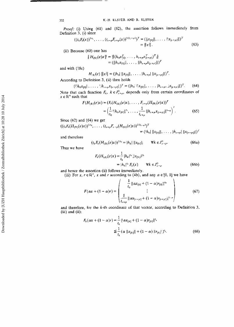
Proof: (i) Using (61) and (62), the assertion follows immediately from Definition 3, (i) since

((toFo(x))"'? ,. . . , (ts+pFs+p(~))l""+P')T = ( I l~~o~ l l , . . . , I I X [ ~ + ~ J I I ) ~ = lllx I l l . (63)

According to Definition 3, (ii) then holds

(Ilho~,o]ll, . . . , Ilhs+p~[s+p]ll)~ = (lhol II~[0lll, . . . , Ihs+pl Ilx[s+p,ll)T (64) Note that each function Fk, k E J:+,, depends only from certain coordinates of x E Rn such that

and hence the assertion (ii) follows immediately. (iii) For x, r E Rn, x and r according to (4b), and any a E [O, 11 we have

and therefore, for the k-th coordinate of that vector, according to Definition 3, (iii) and (ii):

Dow

nloa

ded

by [

UZ

H H

aupt

bibl

ioth

ek /

Zen

tral

bibl

ioth

ek Z

üric

h] a

t 10:

28 1

0 Ju

ly 2

014

VECTOR APPROXIMATION PROBLEMS 333

Since

u k : = c u l l x [ k ] l i + ( l - c u ) l l r [ k l l l ~ o v k ~ J ; + p , each function u t is convex if tk > 1, k E J;+p. Then we obtain from (68)

&(ax + (1 - ( Y ) T ) 5 M k ( x ) + (1 - cY)Fk(r) V k E J:+p and hence follows finally

EZ(&(x) + (1 - a)F(r ) - F(ax + (1 - cu)r)) E [W;+',

i.e. F is RY1-convex. (iv) Because tk > 1 V k E J : + ~ , differentiability of Fk on Rn is obvious. .

Remark: If the index set J:+, is a singleton, then from Lemma 2 a known result of Duffin/Peterson/Zener can be concluded as special case (cf. [3], p. 224).

Now the lemmas proved above will be used as a basis for deriving a special geometric vector inequality which is of importance for a class of geometric vector optimization problems.

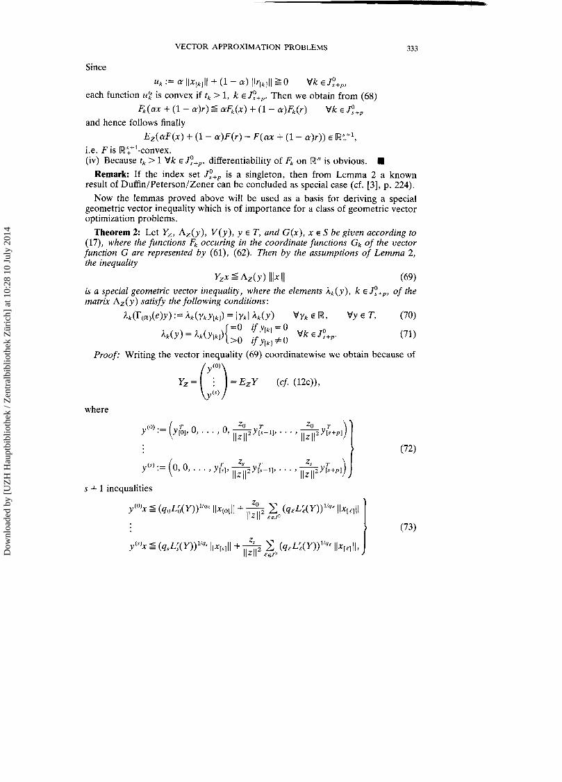
Theorem 2: Let Yz, A z ( y ) , V ( y ) , y E T, and G ( x ) , x E S be given according to (17)) where the functions Fk occuring in the coordinate functions Gk of the vector function G are represented by (61), (62). Then by the assumptions of Lemma 2, the inequality

yzx s AZ(Y lllx I l l (69) is a special geometric vector inequality, where the elements Ak(y), k E J f + p , of the matrix A,(y) satisfy the following conditions:

Proof: Writing the vector inequality (69) coordinatewise we obtain because of

Y z = ( i ' " ) = E z Y ( c . (12c)),

where

s + 1 inequalities

Dow

nloa

ded

by [

UZ

H H

aupt

bibl

ioth

ek /

Zen

tral

bibl

ioth

ek Z

üric

h] a

t 10:

28 1

0 Ju

ly 2

014

334 K.-H. ELSTER AND R. ELSTER

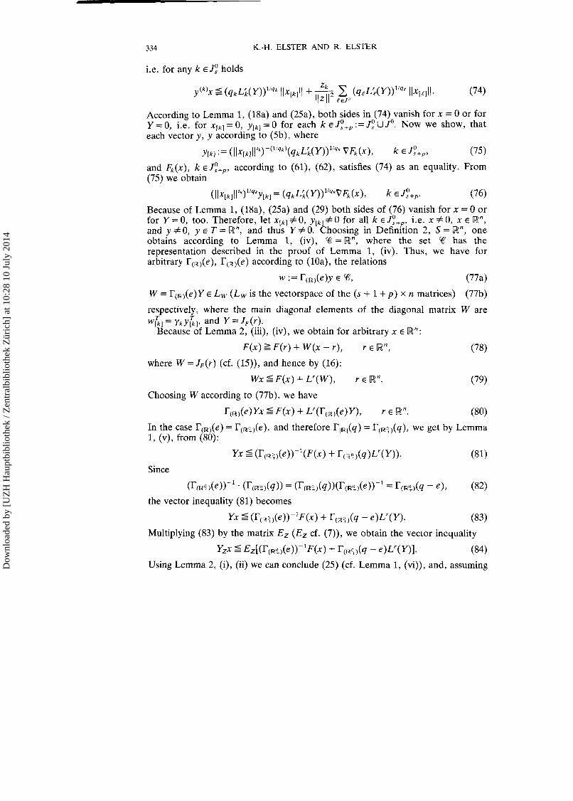
i.e. for any k E J: holds

According to Lemma 1, (18a) and (25a), both sides in (74) vanish for x = 0 or for Y = 0, i.e. for xlk1 = 0, ylk1 = 0 for each k E Jy+p := J: U J'. Now we show, that each vector y, y according to (5b), where

and Fk(x), k E J:+p, according to (61), (62), satisfies (74) as an equality. From (75) we obtain

Because of Lemma 1, (Ma), (25a) and (29) both sides of (76) vanish for x = 0 or for Y = 0, too. Therefore, let X [ ~ ] # 0, Y[k] # 0 for all k E J:+p, i.e. x # 0, x E [Wn, and y # 0, y E T = Rn, and thus Y # 0. Choosing in Definition 2, S = Rn, one obtains according to Lemma 1, (iv), % = Rn, where the set % has the representation described in the proof of Lemma 1, (iv). Thus, we have for arbitrary T(,,(e), r(,,(e) according to (lOa), the relations

W = TcR,(e)Y E Lw (Lw is the vectorspace of the (s + 1 + p ) x n matrices) (77b) respectively, where the main diagonal elements of the diagonal matrix W are w&] = yky;], and Y =

Because of Lemma 2, (iii), (iv), we obtain for arbitrary x E Rn:

F(x) L F(r) + W(x - r), r E Rn, (78) where W = JF(r) (cf. (15)), and hence by (16):

Wx 5 F(x) + Lr(W), r E Rn. (79)

Choosing W according to (77b), we have

T(,,(e) Yx 5 F(x) + Lr(T(,,(e) Y), r E R ". (80) In the case TcR,(e) = T(Rl:)(e), and therefore T,,,(q) = T(,:,(q), we get by Lemma 1, (v), from (80) :

Yx 5 (r(rw'!,(e))-'(F(x) + T(rw?,(q)Lr(Y)). (81) Since

(r(R%)(e>>-l ' (r(~$)(q)) = (r(R%)(q))(T(R%)(e))-l = T ( ~ % ) ( q - (82) the vector inequality (81) becomes

Yx S (T(,:,(e))-'~(x) + T(,%,(q - e)Lr(Y). (83) Multiplying (83) by the matrix Ez (Ez cf. (7)), we obtain the vector inequality

Yzx 5 Ez[(qR%,(e))-*F(x) + qR:,(q - e)Lr(Y)I. (84) Using Lemma 2, (i), (ii) we can conclude (25) (cf. Lemma 1, (vi)), and, assuming D

ownl

oade

d by

[U

ZH

Hau

ptbi

blio

thek

/ Z

entr

albi

blio

thek

Zür

ich]

at 1

0:28

10

July

201

4

VECTOR APPROXIMATION PROBLEMS 335

x # 0, Y # 0, we have F(x) > 0 and Lr(Y) > 0. The vector inequalities (83), (84) become vector equalities, if

Y = (T(~%,(~))- 'W = (r(,$,(e))-'J,(x). (85) Indeed, by Lemma 1, (v) and (82) follows from (83), (84):

(rcrw$,(e)>-lWx 5 (ha,(e))- 'F(x) + (r(rw'?,(q - e))(qIw(:,(q)>-'LX(w)

= (r(w:,(e>)-'[F(x> + LX(W)I,

and therefore

WxS F(x) + Lx(W) resp. I for any x E Rn, W = J,(X). (86) WZx 5 EZ[F(x) + Lx(W)]

Regarding (16), we obtain the assertion. Considering (83) and (85) coor- dinatewise, we have for the kth coordinate of (83):

resp. for the kth main-diagonal element y$l of (85):

where each Fk(x), k E J:+,, is represented by (61), (62). The expression on the right-hand side of (87), considered as a function of yk, has obviously a minimum. Because of qk > 1 (cf. (17d)), Fk(x) > 0 and L;(Y) > 0 for each k E J:,,, we obtain the minimizer

Using yl, k E J:,,, in (87), (88) and taking into consideration assumption (17d), we get

= (tk F ~ ( x ) ) " ~ ~ ( ~ ~ ( L ; ( Y ) ) ~ ~ ~ * V k E J,O+,,

where (90) is an equality, if (cf. (88), (89))

Dow

nloa

ded

by [

UZ

H H

aupt

bibl

ioth

ek /

Zen

tral

bibl

ioth

ek Z

üric

h] a

t 10:

28 1

0 Ju

ly 2

014

336 K.-H. ELSTER AND R. ELSTER

From (90) we obtain immediately

according to (17b), YX s A ( ~ ) G ( x ) { ~ ( Y ) G(x) according to (17c)

and therefore, because of (63):

respectively

Yzx = EzYx 5 EZNY) Ilk Ill = Az(Y) Ilk Ill. (92b) T T If y = ( ~ h , . . . , yl,+,l) , y[,, according to (91), k e J:,,, and thus

Y =~diag(ylkl),E,~+p, then the inequalities (74) and (92) are equalities. Finally, to prove that (92b) is a geometric vector inequality according to

Definition 1 it remains to show that all considerations up to now are valid also in the case that x E R n will be replaced by x E S, S according to (17a), and each element /Zk(y), k E J;,,, in the matrix A(y) (cf. (17b)) is nonnegative on T = Rn.

Now, we choose a vector x E S and a vector d E Rn, x and d according to (4b), such that

d = VF(x), VF(x) according to (22), (93)

i.e. (cf. (4b)):

drkl = V&(X[,]) = V&(X) V k E J:+,. (94)

Then, by (91) and (34b), we have for all k E J:+, the relation

( t&(~))~ '~*d[k] = (V~kT(~)x[k])ll~~d[k]

= (d;p[k])liqkd[k] (95)

and, using additionally (16) and (17d), one gets

Comparing (95) and (96), we obtain

x E S, D = diag(d&l)kEJq+,. Multiplying (97) by y, 2 0, k E J:,,, it follows because of the homogeneity property (53) for each k E J:+,:

Together with (91) it follows in (90) and (92) equality for x E S, ylk1 := ykdlkl V k E J:,,, i.e. Y = TD, T according to (8). For each element of the matrix A(.), A(.) according to (17b), and taking into consideration (9), one has:

Dow

nloa

ded

by [

UZ

H H

aupt

bibl

ioth

ek /

Zen

tral

bibl

ioth

ek Z

üric

h] a

t 10:

28 1

0 Ju

ly 2

014

VECTOR APPROXIMATION PROBLEMS 337

and by Lemma 1, (53), it follows relation (70):

Because of Lemma 1, (vi), we have

and therefore

i.e. relation (71) is valid. Finally, each coordinate function Gk :S+ R, k E J,O+p, of the vector function

G : S + Rs+l+p , where Gk(x) := (tkFk(x))lirk = ( ( x [ ~ ] ( ( Vk E J:+p, is differentiable on the open convex set S, S according to (17a). Therefore, (92b), i.e. (69), satisfies Definition 1 and the proof of Theorem 2 is now complete.

Remark: Replacing in Theorem 2 the vector x E S by

the vector inequality (69) becomes immediately

Yzxl 5 AZ(~)(lllf + xllll - c) - (Yzf - A z ( Y > ~ ) , C E [WS+'+P + > (101)

which is also a geometric vector inequality because of the translation property (14).

4. SPECIAL GEOMETRIC VECTOR OPTIMIZATION PROBLEMS

By the geometric vector inequality according to Definition 1 the following pair of dual geometric vector optimization problems can be introduced (cf. [9]). (P) (Primal geometric vector optimization problem):

G(x)-, v - min x E B := {X E R* 1 x E 9 n s, G(X) 5 0),

where

G(x) := (Gdx), . . . , G,(x))~, G(x) := (Gs+l(x), . . . , Gs+p(~))T G(x) := (G(x)~, G ( X ) ~ ) = according to (4c),

9 c Rn a linear subspace, O < dim 9 = m < n.

( P * ) (Dual geometric vector optimization problem):

V(y) + v - max

y :=y(z) E B* := U B:, z eint R Y ' D

ownl

oade

d by

[U

ZH

Hau

ptbi

blio

thek

/ Z

entr

albi

blio

thek

Zür

ich]

at 1

0:28

10

July

201

4

338 K.-H. ELSTER AND R. ELSTER

where

V(y) := EzV(y), V(y) according to (5c), 9' the orthogonal complement of P, B,* := {y E R" ( y E TI A1(y) = El, Y ~ Z E P).

Weak and strong duality assertions concerning (P), ( P " ) are given in [9], [lo]. Now, we discuss three special geometric vector optimization problems,

so-called vector approximation problems, which are related to certain nonsmooth vector optimization problems. The approach is based on the special geometric vector inequalities (69) and (101).

At the first we consider the "best" approximation of a given vector function, defined by an analytical expression, by a surrogate vector function (vector curve fitting problem). Choosing this "best approximation function" as a linear combination of given vector functions with variable coefficients, where the coefficient vector satisfies certain constraints, we can introduce in (69) the coordinates of the vector x E S , x according to (4b), S according to (17a) as follows:

m

xi := fk(ui) - hF(ui)rj Vi E [k], k E J:+p. j= l

(104)

Here, fk : D + R and hk : D - Rm, k E Jy+p, are any functions, given at fixed, but arbitrary points ui E D, i E [k], k E J:+,, and D is the common domain of definition of all these functions. To simplify notation, let

fk :=fk(~i) , i E [k], k E J,O+~, and

(105)

a, := -hf(ui), i E [k], k E J,O+p, j E Jm. (106)

Then, (104) becomes m

xi = f" + aVrj, i E [k], k E J;+,, j=1

(107)

and therefore

where the (n, - m, + 1) x m-matrix A,,, is defined according to

and the row-vectors a(,) are

a := ( a , . . . a ) , i E [k], k E J:+,.

Setting in (107)

Dow

nloa

ded

by [

UZ

H H

aupt

bibl

ioth

ek /

Zen

tral

bibl

ioth

ek Z

üric

h] a

t 10:

28 1

0 Ju

ly 2

014

VECTOR APPROXIMATION PROBLEMS 339

we obtain from (108):

X[k] =Ak] + xik], k E J:+P. (I12)

Using (108) and (112) we get the "deviation vector"

x = f + A r = f + x l , x , x ' accordingto(4b). (113)

The vector f has fixed coordinates according to (105), and because of (106) we have

A =

By the geometric vector inequality (101), the problem (P) takes the form

(C - P ) (Primal vector curve fitting problem):

111 F + X' 1 1 1 -, v - min (115) X I E B := {x' E [ W n I X I = (x tT , f r T ) E 9 n s l ,

x ' according to (4b), S ' according to (loo),

1/17 + i'111 5 c, c E RP, constant) with

where

9 is the column space of matrix A, A according to (114). Dow

nloa

ded

by [

UZ

H H

aupt

bibl

ioth

ek /

Zen

tral

bibl

ioth

ek Z

üric

h] a

t 10:

28 1

0 Ju

ly 2

014

340 K.-H. ELSTER AND R. ELSTER

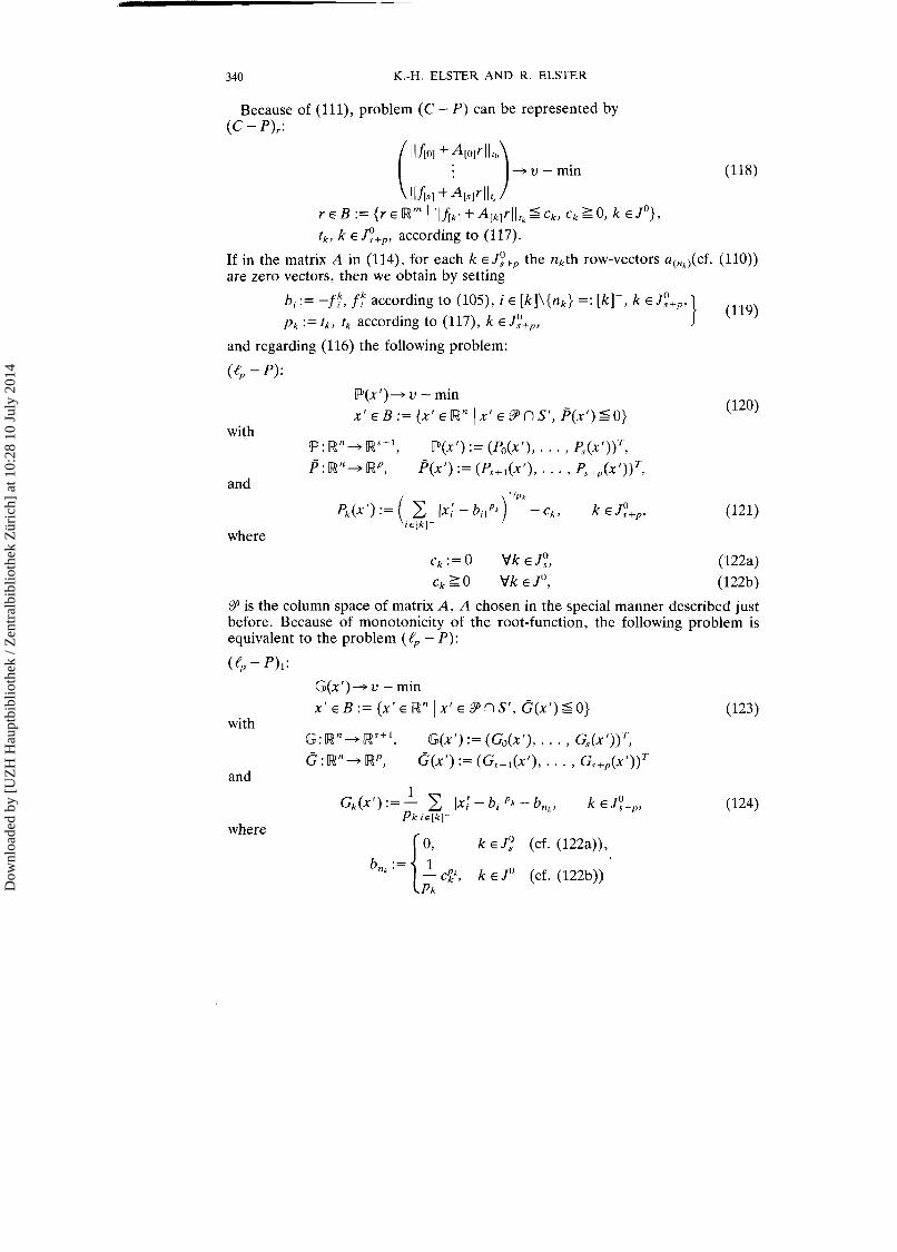
Because of ( I l l ) , problem (C - P) can be represented by (C - P),:

If in the matrix A in (114), for each k E J:+, the nkth row-vectors a(,,,(cf. (110)) are zero vectors, then we obtain by setting

bi := -ff, f: according to (105), i E [k]\{nk> =: [k]-, k E J:+p, pk := fk, fk according to (117), k E J:,,,

and regarding (116) the following problem:

P(xl) + v - min x l ~ B : = { x ' ~ j W n ) x r E P ~ S ' , P(xl)SO) (120)

with P : [ W n + [Ws+l, P(xl) := (Po(xl), . . . , P,(x'))~, P : R n + [Wp, P(xl) := (P,+~(X~), . . . , Ps+p(xr))T,

and

P? is the column space of matrix A, A chosen in the special manner described just before. Because of monotonicity of the root-function, the following problem is equivalent to the problem (lp - P):

G(xl) + v - min x 1 ~ B : = { x 1 ~ [ W n I X I E P n s l , G ( x l ) s o )

with G:Rn+ [WS+l, G(xl) := (Go(xl), . . . , G,(x'))~,

: 58''- Rp, G(xl) := ( G ~ + ~ ( X ' ) , . . . , Gs+p(xl))T and

where ( 0, k E J; (cf. (122a)),

- cP,", k E Jo (cf. (122b))

Dow

nloa

ded

by [

UZ

H H

aupt

bibl

ioth

ek /

Zen

tral

bibl

ioth

ek Z

üric

h] a

t 10:

28 1

0 Ju

ly 2

014

VECTOR APPROXIMATION PROBLEMS 341

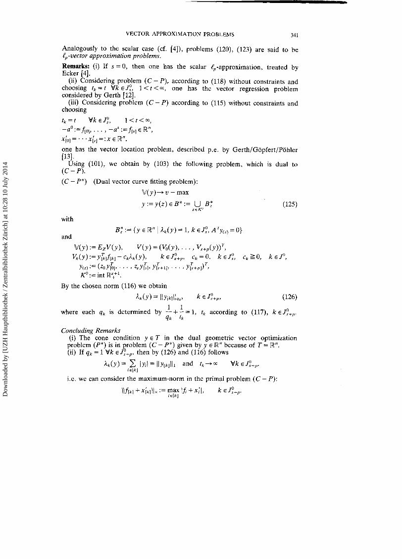
Analogously to the scalar case (cf. [4]), problems (120), (123) are said to be 8,-vector approximation problems.

Remarks: (i) If s = 0, then one has the scalar 8,-approximation, treated by Ecker 141.

(ii) &sidering problem (C - P), according to (118) without constraints and choosing tk = t Vk E J:, 1 < t < a, one has the vector regression problem considered by Gerth [12].

(iii) Considering problem (C - P ) according to (115) without constraints and choosing

t,=t VkEJ:, l < t < m , -a0:=fiO1, . . . , -aS := f[sl E Rn, xfo1=. . . x ~ , ] = : x €Rn ,

one has the vector location problem, described p.e. by GerthlGopfertlPohler [131.

Using (101), we obtain by (103) the following problem, which is dual to (C - P).

(C - P*) (Dual vector curve fitting problem):

V(y) + v - max

with

I?,*:= {y E Rn I Ak(y) = 1, k EJ:, ATy,,,=O) and

By the chosen norm (116) we obtain

1 1 where each qk is determined by -+-= 1, tk according to (117), k E J;+,.

qk tk

Concluding Remarks (i) The cone condition y E T in the dual geometric vector optimization

problem (P*) is in problem (C - P*) given by y E Rn because of T = Rn. (ii) If qk = 1 V k E J:+,, then by (126) and (116) follows

i.e. we can consider the maximum-norm in the primal problem (C - P):

Dow

nloa

ded

by [

UZ

H H

aupt

bibl

ioth

ek /

Zen

tral

bibl

ioth

ek Z

üric

h] a

t 10:

28 1

0 Ju

ly 2

014

342 K.-H. ELSTER AND R. ELSTER

Therefore, the dual vector curve fitting problem can be formulated as a linear vector optimization problem and well-known methods for solving such prob- lems are available.

References

[I] Bacopoulos, A., Godini, G. and Singer, I. (1980) On infima of sets in the plane and best approximation, simultaneous and vectorial, in a linear space with two norms. In: Special Topics of Applied Mathematics, Frehse, J . ; Pallaschke, D.; Trottenberg, U., (Eds.), North Holland, Amsterdam

[2] Bacopoulos, A , , Godini, G. and Singer, I. (1978) On best approximation in vector-valued norms. Colloquia Mathernatica Societatis Ja'nos Bolyai, 19, 89

[3] Duffin, R., Peterson, E . L, and Zener, C. (1967) Geometric Programming-Theory and Application. John Wiley & Sons, New York

[4] Ecker, J. G. (1968) Geometric Programming: duality in quadratic programming and e,- approximation. Dissertation University of Michigan

[5] Elster, R. (1990) Geometrische Vektoroptimierung. Dissertation B, Technische Hochschule Merseburg

[6] Elster, K.-H. and Elster, R . (1988) Approaches to duality of geometric vector optimization. 33. Intern. Wiss. Kolloquium der Techn. Hochschule Ilmenau, H. 4, pp. 27-32

[7] Elster, K.-H. and Elster, R. (1988) Ein Dualitatskonzept fur geometrische Vektorop- timierungsprobleme. Wiss. Schriftenreihe der TU Karl-Marx-Stadt H. 2, pp. 3-12

[8] Elster, K.-H. and Elster, R . (1991), Geometric vector optimization. In: Atti del Quattordicesimo Convegno A.M.A.S.E.S., Pescara, 13-15 Settembre 1990. EDI. PRESS-ROMA 1991, pp. 3-14

[9] Elster, K.-H., Elster, R. and Gopfert, A. (1990) On approaches to duality theory in geometric vector optimization. In: Methods of Operations Research, Vol. 60, pp. 23-37, Anton Hain, MeisenheimIFrankfurt a.M.

1101 Elster, R., Gerth, Chr. and Gopfert, A. (1989) Duality in geometric vector optimization. Optimization 20, 4, 457-477

[11] Gearhart, W. B. (1974) On vectorial approximation. Journal of Approximation Theory 10 pp. 49. [12] Gerth, Chr. (1987) Dualitatsaussagen fur das vektorwertige Regressionsproblem. Aus dem wiss.

Leben der Padag. Hochschule "N. K. Krupskaga" HalleIS., H. 4, pp. 31-34 [13] Gerth, Chr., Gopfert, A. and Pohler, K. (1988) Vektorielles Standortproblem und Dualitat.

Wiss. Zeitschrift Karl Marx-Universitat Leipzig, Math.-Naturwiss. R. 37, H. 4, pp. 305-312 [14] Jahn, J. (1985) Scalarization in multiobjective optimization. In: Mathematics of Multi Objective

Optimization. P. Serafini (Ed.), Universita di Udine. Springer-Verlag, Wien -New York, pp. 45-87

1151 Jahn, J. and Krabs, W. (1988) Applications of multicriteria optimization in approximation theory. In: Multicriteria Optimization in Engineering and in the Sciences, Stadler, W. (Ed.), Plenum Press. New York - London

Dow

nloa

ded

by [

UZ

H H

aupt

bibl

ioth

ek /

Zen

tral

bibl

ioth

ek Z

üric

h] a

t 10:

28 1

0 Ju

ly 2

014