
NASA Contractor Report 4619
Venusian Atmospheric and Magellan PropertiesFrom Attitude Control Data
Christopher A. Croom and Robert H. Tolson
The George Washington University, Joint Institute for Advancement of Flight Sciences,
Langley Research Center • Hampton, Virginia
National Aeronautics and Space AdministrationLangley Research Center • Hampton, Virginia 23681-0001
Prepared for Langley Research Center
under Cooperative Agreement NCC1-104
August 1994
https://ntrs.nasa.gov/search.jsp?R=19950005278 2018-05-28T19:37:10+00:00Z


Abstract
Results are presented of the study of the Venusian atmosphere, Magellan
aerodynamic moment coefficients, moments of inertia, and solar moment coefficients.
This investigation is based upon the use of attitude control data in the form of reaction
wheel speeds from the Magellan spacecraft. As the spacecraft enters the upper
atmosphere of Venus, measurable torques are experienced due to aerodynamic effects.
Solar and gravity gradient effects also cause additional torques throughout the orbit. In
order to maintain an inertially fixed attitude, the control system counteracts these torques
by changing the angular rates of three reaction wheels. Model reaction wheel speeds are
compared to observed Magellan reaction wheel speeds through a differential correction
procedure.
This method determines aerodynamic, atmospheric, solar pressure and mass
moments of inertia parameters. Atmospheric measurements include both base densities
and scale heights. Atmospheric base density results confirm natural variability as
measured by the standard orbital decay method. Potential inconsistencies in free
molecular aerodynamic moment coefficients are identified. Moments of inertia are
determined with a precision better than 1% of the largest principal moment of inertia.
PAGE BLANK NOT FILMEDiii

Table of Contents
Abstract ............................................................................................................................ iii
Table of Contents ............................................................................................................. iv
List of Figures .................................................................................................................. v
List of Tables ................................................................................................................... vi
Nomenclature ................................................................................................................... vii
Abbreviations ................................................................................................................... ix
I. Introduction ................................................................................................................. 1
1. Purpose of Study ............................................................................................. 1
2. Previous Work ................................................................................................ 2
3. Report Organization ........................................................................................ 2
II. Magellan Spacecraft ................................................................................................... 2
1. Vehicle Description ........................................................................................ 2
1.1. Spacecraft ......................................................................................... 2
1.2. Attitude and Articulation Control System ....................................... 4
1.3. Reaction Wheels .............................................................................. 4
1.4. Tachometers ..................................................................................... 5
2. Mission Description ........................................................................................ 6
3. Orbit Description ............................................................................................ 6
4. Data Requirements .......................................................................................... 7
III. Reaction Wheel Speed Model ................................................................................... 8
1. Introduction ..................................................................................................... 8
2. Atmospheric/Aerodynamic Torques .............................................................. 9
3. Gravity Gradient Torques ............................................................................... 15
4. Solar Pressure Torques ................................................................................... 17
5. Neglected Torques .......................................................................................... 18
6. Final Reaction Wheel Speed Model and Parameters ...................................... 19
IV. Differential Correction .............................................................................................. 21
1. Introduction ..................................................................................................... 21
2. Parameters ....................................................................................................... 22
3. A Priori ............................................................................................................ 23
4. Iteration and Convergence .............................................................................. 23
5. Cramer-Rao Bounds ....................................................................................... 24
V. Results ........................................................................................................................ 24
1. Introduction ..................................................................................................... 24
2. Atmospheric / Aerodynamic Parameters ........................................................ 25
2.1. Base Density Method ....................................................................... 26
2.1.1. Base Density ..................................................................... 26
2.1.2. Yaw and Roll Aerodynamic Moment Coefficients .......... 28
2.2. Scale Height Method ....................................................................... 30
2.2.1. Scale Heights .................................................................... 31
2.2.2. Yaw and Roll Aerodynamic Moment Coefficients .......... 36
3. Mass Moments of Inertia ................................................................................ 37
4. Solar Pressure Moment Coefficients .............................................................. 43
iv

VI.
1.
2.
3.
4.
5.
6.
Accuracy Analysis .................................................................................................... 47Introduction ..................................................................................................... 47
Base Densities ................................................................................................. 48
Yaw and Roll Aerodynamic Moment Coefficients ........................................ 49
Scale Height Correction Factors ..................................................................... 52
Mass Moments of Inertia ................................................................................ 54
Solar Moment Coefficients ............................................................................. 55
VII. Conclusion ............................................................................................................... 57
1. Atmospheric .................................................................................................... 57
2. Aerodynamic ................................................................................................... 573. Mass Moments of Inertia ................................................................................ 58
4. Solar Moment Coefficients ............................................................................. 58
VIII. Future Work ........................................................................................................... 59
Appendices ...................................................................................................................... 60
A. Reaction Wheel Speed Integral ...................................................................... 60
B. Differential Correction General Equation ...................................................... 61
C. Model of Solar Array Mass Moments of Inertia ............................................ 62
D. Magellan Attitude Control Data Analysis Software (MACDAS) ................. 63
E. Cycle Four History ......................................................................................... 73
F. Reaction Wheel Data Logistics ...................................................................... 79
References ........................................................................................................................ 81
List of Figures
1.1 The Magellan Body-Fixed Coordinate System ......................................................... 3
3.1 VIRA Density at Three Local Solar Times ............................................................... 10
3.2 VIRA Scale Heights at Three Local Solar Times ..................................................... I 1
3.3 Reaction Wheel Speed Due to Atmospheric Torque ................................................ 11
3.4 Freemac Pitch Aerodynamic Moment Coefficients (Before Conjunction) .............. 12
3.5 Freemac Pitch Aerodynamic Moment Coefficients (After Conjunction) ................. 13
3.6 Freemac Yaw Aerodynamic Moment Coefficients for Three Orbits ........................ 14
3.7 Freemac Pitch Aerodynamic Moment Coefficients for Three Orbits ....................... 14
3.8 Freemac Roll Aerodynamic Moment Coefficients for Three Orbits ........................ 14
3.9 Reaction Wheel Speed Due to Gravity Gradient Torque .......................................... 16
3.10
3.11
5.1
5.2
5.3
5.4
5.5
5.6
5.7
5.8
Reaction Wheel Speed Due to Solar Pressure Torque ............................................ 18
Example Contributions to Pitch Reaction Wheel Speed ........................................ 20
Reaction Wheel Speed for Orbit #7610 .................................................................... 25
Density as Determined By Reaction Wheel Method and Drag Method ................... 27
Reaction Wheel and Drag Method Base Density Between 9 AM and 10 AM ......... 27
Yaw Aerodynamic Moment Coefficient ................................................................... 28
Roll Aerodynamic Moment Coefficient ................................................................... 29
Scale Height Correction Effect on Residuals of Orbit #7511 ................................... 32
Scale Height Correction Effect on Residuals of Orbit #7479 ................................... 32
VIRA and Recovered Scale Heights (19 ° to 11 ° North Latitude) ............................ 33

5.9
5.10
5.11
5.12
5.13
5.14
5.15
5.16
5.17
5.18
5.19
5.20
5.21
5.22
5.23
5.24
VIRA and Recovered Scale Heights (11 ° to 3° North Latitude) .............................. 34
Scale Height Correction Factor Sensitivity to Time of Periapsis Error .................. 35
Yaw Aerodynamic Moment Coefficient for Orbit #7503 ....................................... 36
Roll Aerodynamic Moment Coefficient for Obit #7503 ......................................... 37
Model Mass Moment of Inertia Iyy of Magellan Solar Arrays ............................... 38
Estimated Mass Moment of Inertia Iyy of Spacecraft Bus ..................................... 38
Model Mass Moment of Inertia Izz of Magellan Solar Arrays ............................... 39
Estimated Mass Moment of Inertia Izz of Spacecraft Bus ...................................... 39
Model Mass Product of Inertia Iyz of Magellan Solar Arrays ................................ 40
Estimated Mass Product of Inertia Iyz of Spacecraft Bus ....................................... 40
Estimated Mass Product of Inertia Ixy of Spacecraft Bus ...................................... 41
Estimated Mass Product of Inertia Ixz of Spacecraft Bus ...................................... 41
Solar Longitude and Latitude Definition ................................................................ 43
Cycle Four Solar Longitude and Latitude ............................................................... 44
Estimated Yaw Solar Moment Coefficient for Cycle Four .................................... 45
Estimated Pitch Solar Moment Coefficient for Cycle Four .................................... 46
5.25 Estimated Roll Solar Moment Coefficient for Cycle Four ..................................... 47
6.1 Normalized Base Density Accuracy Estimate .......................................................... 48
6.2 Yaw Aerodynamic Moment Coefficient Accuracy Estimate .................................... 50
6.3 Roll Aerodynamic Moment Coefficient Accuracy Estimate .................................... 50
6.4 Yaw and Roll Aerodynamic Moment Coefficient Sample Standard Deviation ....... 51
6.5 Scale Height Correction Accuracy (19 ° to 11 ° North Latitude) ............................... 52
6.6 Scale Height Correction Accuracy (11 ° to 3 ° North Latitude) ................................. 53
6.7 Solar Moment Coefficient Accuracy ......................................................................... 55
6.8 Solar Moment Coefficient Sample Standard Deviation ........................................... 56
List of Tables
2.1 Reaction Wheel Specifications ................................................................................. 5
4.1 Data Requirements for Model Parameters ................................................................ 22
4.2 Spacecraft Bus Moments of Inertia A Priori ............................................................. 24
5.1 Spacecraft Bus Mean Estimated Moments of Inertia ............................................... 42
5.2 Magellan Spacecraft Total Moments of Inertia ........................................................ 42
6.1 Spacecraft Bus Estimated Moments of Inertia Accuracy ......................................... 54
vi

Nomenclature
A
A
s
ArF-IAn f -n
b
Cm d
Cm ._
C
g
h
h o
H
n s
i ,j,k
Irw
J
l,m,n
L
t_
m
m lt
solar array width, m
sensitivity matrix
reference area for atmospheric torque, m 2
reference area for solar torque, m"
information matrix
solar array length, m
aerodynamic moment coefficient
solar moment coefficient
constant
gravitational acceleration, m/s 2
altitude, km
base altitude, km
angular momentum, kg.m2/s
scale height, km
unit vectors in spacecraft coordinate system
spacecraft mass moment of inertia, kg.m 2
reaction wheel moment of inertia for axis of rotation, kg.m 2
cost function
direction cosines
reference length for aerodynamic torque, m
reference length for solar torque, m
solar array mass, kg
atmospheric atomic mass
vii

M
n
N
P
P
R
R"
t
T
L
L
7.
v
x
x,.,Yc,Zc
y
O_
Fx
FE
0
_X
9
number of parameters
iteration number
number of data points
solar momentum flux, kg/(m.s 2)
generic parameter
spacecraft radial distance from Venus center of attraction, m
universal gas constant, kJ/(kgmol.K)
time index
environmental torque, N.m
atmospheric torque, N.m
gravity gradient torque, N.m
solar pressure torque, N.m
atmospheric temperature, °K
spacecraft velocity, m/s
parameter state vector
center of mass location in spacecraft coordinates, m
observed reaction wheel speed, rad/sec
scale height correction factor
angle between roll axis and solar array surface, degrees
a priori covariance matrix
measurement covariance matrix
residuals, rad/sec
angle between roll axis and active solar array normal,
degrees
a priori estimates
Venus gravitational constant, m3/s 2
atmospheric density, kg/m 3
viii

13 E
(Yx
0,)
atmospheric base density, kg/m 3
measurement standard deviation
a priori standard deviation
model reaction wheel speed, rad/sec
Abbreviations
AACS
ARU
Freemac
LST
MACDAS
VIRA
Attitude and Articulation Control System
Attitude Reference Unit
Free molecular flow simulation software
Local Solar Time
Magellan Attitude Control Data Analysis Software
Venus International Reference Atmosphere
ix


I. INTRODUCTION
1.1 Purpose of Study
The purpose of this research is to develop an alternate technique to the standard
orbital decay method I to determine Venusian atmospheric densities. This technique was
used to confirm the large natural variability in atmospheric density observed by the orbital
decay measurements prior to the Magellan aerobraking experiment 2'3. In addition to
density, atmospheric scale heights, spacecraft aerodynamic moment coefficients, solar
moment coefficients, and mass moments of inertia are also determined. This technique
uses attitude control data from the Magellan spacecraft in the form of reaction wheel
speeds. This work is a continuation of a feasibility study done by Marsden and Croom 4'5
and extends results presented by Croom and Tolson 6.
The reaction wheel method presents several advantages to the orbital decay
method of determining atmospheric densities. This orbital decay method is based on the
use of Doppler shift measurements. Using reaction wheel data eliminates the "plane of
sky" problem ,inherent in Doppler shift measurements, and has the ability to determine
spatial atmospheric variation on each orbit. For one orbit, the decay method is limited to
base density determination whereas the reaction wheel data contains density variation
information that represents scale heights and/or latitudinal variation. Since the Magellan
spacecraft does not have the ability to record reaction wheel speeds, all data must be
transmitted to Earth as it is observed. On the other hand, Doppler results can be obtained
without spacecraft communication at periapsis.
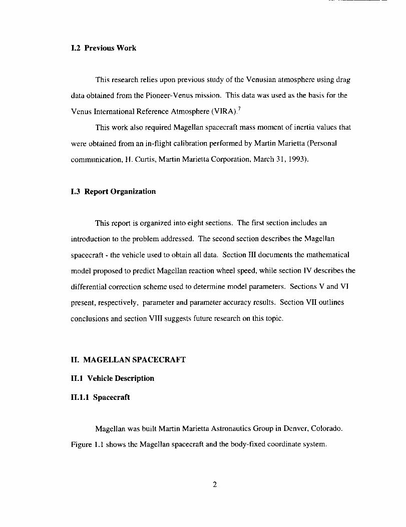
1.2 Previous Work
This research relies upon previous study of the Venusian atmosphere using drag
data obtained from the Pioneer-Venus mission. This data was used as the basis for the
Venus International Reference Atmosphere (VIRA). 7
This work also required Magellan spacecraft mass moment of inertia values that
were obtained from an in-flight calibration performed by Martin Marietta (Personal
communication, H. Curtis, Martin Marietta Corporation, March 31, 1993).
1.3 Report Organization
This report is organized into eight sections. The first section includes an
introduction to the problem addressed. The second section describes the Magellan
spacecraft - the vehicle used to obtain all data. Section III documents the mathematical
model proposed to predict Magellan reaction wheel speed, while section IV describes the
differential correction scheme used to determine model parameters. Sections V and VI
present, respectively, parameter and parameter accuracy results. Section VII outlines
conclusions and section VIII suggests future research on this topic.
II. MAGELLAN SPACECRAFT
II.1 Vehicle Description
II.l.1 Spacecraft
Magellan was built Martin Marietta Astronautics Group in Denver, Colorado.
Figure 1.1 shows the Magellan spacecraft and the body-fixed coordinate system.

Yaw
Roll
Figure 1.1 The Magellan Body-Fixed Coordinate System
The roll direction is defined by a vector pointing in the nominal direction of the high gain
antenna boresight. The yaw axis is coincident with the solar array axis of rotation. The
positive sense of this direction is defined by the spacecraft side with the altimeter antenna.
The pitch axis completes a yaw, pitch, roll, right-handed system. A reaction wheel is
located along each of these three directions. Under normal conditions, the roll axis points
to Earth. The spacecraft is then rolled so that the yaw axis is normal to the spacecraft-sun
line. Finally, the solar arrays are rotated about the yaw axis so as to be normal to the
spacecra_-sun line. This specification uniquely determines the attitude of the spacecraft
and solar array position at periapsis. Under this configuration, the spacecraft velocity
vector is generally within 15° of the yaw axis at periapsis During a large portion of Cycle

large portion of Cycle Four, a 10 ° Earth-point roll was implemented (i.e., spacecraft is
rotated +10 ° about the roll axis) for mission thermal constraints. An x-y-z system is also
used such that +x coincides with Yaw, +y is Pitch, and +z is Roll.
II.1.2 Attitude and Articulation Control System
Magellan attitude is controlled by the Attitude and Articulation Control System
(AACS). The AACS maintains the inertially fixed attitude, described in section 1.4,
during periapsis and points the spacecraft in any required direction as dictated by mission
requirements. Attitude adjustments are necessary for mapping, communications, star
tracker scans, and momentum desaturations. The spacecraft is 3-axis stabilized by both
reaction control thrusters and reaction wheels. Since only reaction wheels are used during
periapsis events of Cycle Four, only that attitude control data is relevant to this study.
Attitude is measured by gyroscopes within the Attitude Reference Unit (ARU).
This attitude is updated by a star tracker scan on each orbit and is recorded by a set of
four Euler parameters, or quaternions. These quaternions uniquely define spacecraft
attitude referenced to the J2000 inertial reference frame. 8 Quaternions are used to
calculate the transformation matrix necessary to convert coordinates from the J2000
system into the Magellan body-fixed coordinate system with no physical singularities. 9
II.1.3 Reaction Wheels
By changing the speed of the reaction wheels, the AACS controls the angular
momentum of the spacecraft. By conservation of angular momentum (in the absence of
external torques) changes in the speed of these wheels must be accompanied by changes
in spacecraft angular rates. In this manner, Magellan attitude and angular rates are
controlled. In a similar fashion, when the spacecraft experiences environmental torques,
4

AACS mustchangetheangularratesof thereactionwheelsin order to maintain an
inertially fixed attitude. Angular momentum is thus transferred and stored within the
reaction wheels. This angular momentum is removed from the reaction wheels during
desaturation maneuvers. During these desaturation maneuvers, thrusters are used to exert
a net moment on the spacecraft such that the reaction wheels must slow down in order to
counteract the thruster moment. Reaction wheel specifications are give in Table 2.1
(Personal communication, Mike Nicholas, Honeywell Satellite Systems, Inc., March 16,
1993).
Stiction < 0.01 N.m
Maximum Angular Rate
Maximum Torque Output
Measurement Quantization
Principal Moment of Inertia
Maximum Momentum Storage
Maximum (Peak) Power Usage
Time to Switch Torque Direction
470 rad/s
0.18 N.m
1.0236 rad/s/bit
0.06638 kg.m 2
27.0 N.m.s
145 W
<0.1s
Table 2.1 Reaction Wheel Specifications
11.1.4 Tachometers
Two redundant tachometers are used to measure the speed of each reaction wheel.
These devices rely on Hall effect sensors and commutators. Measurement of wheel speed
is quantized to 1.0236 rad/s/bit by the tachometers. The sensors detect changes in the
5

local magnetic field caused by the passing commutator and can therefore determine the
angular velocity of the reaction wheel.
Although speed is quantized to 1.0236 tad/s/bit, the noise level of the
measurement signal may be much larger. At low reaction wheel speeds, measurements
tend to lie within a range of + 2.6 rad/s. This is much larger than the range of + 0.5118
rad/s that the reaction wheel demonstrates at higher speeds. This anomaly is attributed to
"stiction" or "dynamic friction" within the reaction wheel assembly.
II.2 Mission Description
The Magellan spacecraft was launched from the space shuttle Atlantis, STS-30,
on May 4, 1989. After reaching Venus in August of 1990, the primary mission of
mapping the planet surface continued for three Venusian sidereal days. Over 97% of the
planet's surface was mapped through the use of synthetic aperture radar. _° September 15,
1992, marked the beginning of Cycle Four, the fourth sidereal day, which was reserved
for gravitation field analysis. In addition, atmospheric studies were included to confirm
atmospheric and aerodynamic properties prior to aerobraking. A series of aerobraking
maneuvers was executed at the conclusion of Cycle Four to circularize the Magellan
orbit. This new orbit would allow greater resolution in gravity measurements near the
Venus poles. 11
II.3 Orbit Description
During Cycle Four, Magellan was in a nearly polar orbit with an eccentricity of
0.39. Periapsis altitude ranged from 165 km to 185 km and the orbital period was 3.25
hours. Argument of periapsis and longitude of the ascending node were such that the
spacecraft approached periapsis, which occurred at approximately 11 ° north latitude,
6

from theVenusNorthPole. Undertheseconditions,atmospherictorquesaredetectable
by the control system for up to 200 seconds during the periapsis event. The first orbit of
Cycle Four was orbit #5754 that occurred on September !5, 1992, and the final orbit was
orbit #7626 that occurred on May 26, 1993. This study represent a complete analysis of
Cycle Four. (See Appendix E for more complete history of spacecraft orbit,
configuration, and geometry during Cycle Four.)
II.4 Data Requirements
Data required for reaction wheel analysis consists of tachometer speeds,
quaternions, and Magellan orbital elements. Orbital elements include semimajor axis,
eccentricity, inclination, longitude of the ascending node, argument of periapsis, and time
of periapsis. Reaction wheel speeds and spacecraft attitude are transmitted from the
spacecraft at either a high or low data rate. For high rate data, reaction wheel speed has a
sample period of 0.667 seconds. In the case of low rate, the sample period is 20 seconds
(see Appendix E, Figure E. 15). High rate transmission is preferable, but not always
available due to mission constraints. In general, reaction wheel speeds and quaternions
are transmitted for a period of time corresponding to twenty minutes before and after
periapsis. The spacecraft attitude can be assumed to be inertially fixed during this time
since the quaternions show no change in the four decimal places recorded by the AACS.
Thus it can be assumed that all net change in spacecraft angular momentum, which is
caused by external torques, is absorbed by the reaction wheels.
Orbital elements are determined from tracking data and an orbit determination
algorithm. The classical orbital elements including time of periapsis are determined for
each orbit. This information is required for orbit simulation.
In order for the reaction wheel method to be implemented, all of the above
described data must be available. Further, the effectiveness of this method is affected by

the quantity of reaction wheel data available for a given orbit. For example, scale height
measurements require data to be transmitted at the high rate, while mass moment of
inertia and solar pressure parameters call for data to extend well beyond the atmospheric
flight phase.
III. REACTION WHEEL SPEED MODEL
III.1 Introduction
In this section, a model for parameter estimation will be postulated and examined
using prior information about the environmental torques and Magellan spacecraft.
Modeled reaction wheel speeds can be compared to observed reaction wheel
speeds in order to determine environmental torques experienced by the Magellan
spacecraft. Modeling reaction wheel speed requires the modeling of all significant
torques and the parameterizing of these models. Significant torques experienced by the
spacecraft are caused by aerodynamic forces, gravity gradients, and solar pressure forces.
Modeling torques caused by these three physical phenomenon will provide an estimate of
the total torque experienced by the spacecraft during a specified time interval. Reaction
wheel speeds are a corollary of these total torques as given by the following equation (see
appendix A).
o_ = Tdt + C (1)
8

I -~ ~-- --~--
111.2 Atmospheric / Aerodynamic Torques
Aerodynamic forces are experienced by Magellan as it enters the Venusian upper
atmosphere. Dynamic pressure at periapsis may approach 1. 7 · 10-4 N / m 2 . Depending
upon spacecraft configuration and relative wind direction , an offset exists between the
center of aerodynamic pressure and spacecraft center of mass. This offset results in a
moment, or torque, due to atmospheric dynamic pressure. Maximum torque caused by
the Venusian atmosphere during Cycle Four was approximately 1. 6 .10-3 N · m .
Aerodynamic torque can be resolved into the three body-fixed axes: yaw, pitch, and roll.
Each component of torque due to atmospheric effects is determined by the relation
(2)
where v is determined from the solution of the two-body problem and p is density. Aa
and La are defined, respectively, as characteristic area (23 m2) and length (3.66 m). The
unknowns are therefore the aerodynamic moment coefficients cmd and the atmospheric
base density. For mission operations, cmd is determined from a free molecular flow
simulation (Freemac) J 2 and p is obtained from the Venusian International Reference
Atmosphere (VIRA). For scientific purposes, p is considered unknown. On the other
hand, if P were known, then three aerodynamic moment coefficients could be determined
since Eq. (2) applies to three independent coordinate axes: yaw, pitch, and roll.
Accordingly, there are three unknown aerodynamic moment coefficients and one
unknown base density. Variation in density near periapsis is modeled through the use of
a piecewise continuous exponential function that matches VIRA densities at five
kilometer intervals. Between these points, density is modeled as
9

(3)
where scale height can be related to atmospheric temperature hy II , == If Til / '" /I g. Tile
atmosphere is therefore divided into five kilometer laye rs. Within each layer, sca le height
is assumed constant. A general, s implified atmospheric st ructure can then be described
by a base density at some altitude and a set of seale heights above the base altit ude. Botl!
dens ity and scale heights are functions of alt itude and local solar time as shown in Figurc~
3. 1 and 3.2.
10
10 10
-"" ~ 11 ~ 10
NOON
~ 1 0 12~
~ :: -: ~ ~I ::-----:-!":;-----:-::-::----::-~' ::-----:::-=-::-----:::-:-:0------:::-: 140 160 180 200 220 240 2 60
. , SIX AM '
I'I IDNIGHT
ALTITUDE (KM)
Figure 3.1 VIRA Density at Three Local Solar Times
~-----,
MIDNIGHT 50
~40
:,IX AM
~- - -- - ~ - --:~c;~ --- .,. :.. -----: ::: - -
160 180 200 220 2 4 0 2 60 ALTl:TUDE (KM)
Figure 3.2 VIRA Scale Heights at Three Local Solar Times
10
-- -----
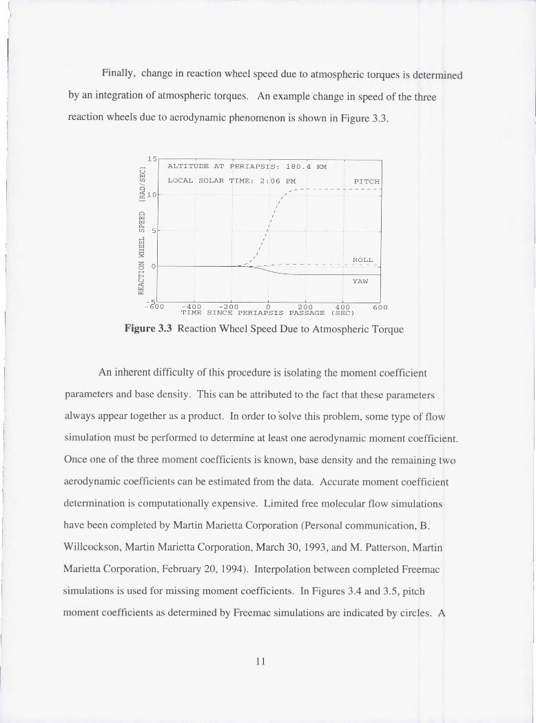
Finally, change in reaction wheel speed due to atmospheric torques is determined
by an integration of atmospheric torques. An example change in speed of the three
reaction wheels due to aerodynamic phenomenon is shown in Figure 3.3.
15,-----~----~----~------~----~----~
u w Ul ...... a ~ 10
a w W a.. U) 5 ...:I I:LI W
~
ALTITUDE AT PERIAPSrS : 180. 4 KM
LOCAL SOLAR TIME: 2 : 06 PM
, I
I
I
I ,
, I
I
, ,
PITCH
ROLL ~ O~----------~~-= .- 7 - - - - ~ -.- - - - - - -
H E-<
~ 0::
YAW
~~0~0~----4~0~0-----2~0~0----~0-----2~0~0~---4~0~0----6~00 TIME SINCE PERIAPS I S PASSAGE (SEC)
Figure 3.3 Reaction Wheel Speed Due to Atmospheric Torque
An inherent difficulty of this procedure is isolating the moment coefficient
parameters and base density. This can be attributed to the fact that these parameters
always appear together as a product. In order to solve this problem, some type of flow
simulation must be performed to determine at least one aerodynamic moment coefficient.
Once one of the three moment coefficients is known, base density and the remaining two
aerodynamic coefficients can be estimated from the data. Accurate moment coefficient
determination is computationally expensive. Limited free molecular flow simulations
have been completed by Martin Marietta Corporation (Personal communication, B.
Willcockson, Martin Marietta Corporation, March 30, 1993, and M. Patterson, Martin
Marietta Corporation, February 20, 1994). Interpolation between completed Freemac
simulations is used for missing moment coefficients. In Figures 3.4 and 3.5, pitch
moment coefficients as determined by Freemac simulations are indicated by circles. A
11

sign change in the pitch aerodynamic moment coefficient occurs near inferior conjunction
when the spacecraft executes a 1800 roll maneuver. For purposes of presentation, these
coefficients are plotted separately for periods before and after conjunction. Solid lines
indicate the interpolation scheme. Discontinuities appear as the result of either spacecraft
rolls or solar array off-point adjustments to satisfy mission thermal constraints (see
Appendix E, Figure E.15) .
::c u
0 . 11
0.1
~ 0 . 09 0..
'0
0 0 . 08
0 . 07
0 . 06~~~~~--6~2~0~0~~6~4~0~0--6~6~0~0--~68~0~0~~7~0~0~0~7~200 ORBIT NUMBER
Figure 3.4 Freemac Pitch Aerodynamic Moment Coefficients (Before Conjunction)
- 0.05
- 0 . 06
::c -0.07 ~ H 0.. -0 .08 '0
0-0.09
-0 .1
- 0 . 11
-0 ·~i~070--~77270~0--~7~3~0~0~~7~4~0~0~~7~5~070--~7~6700~~7~700 ORBIT NUMBER
Figure 3.5 Freemac Pitch Aerodynamic Moment Coefficients (After Conjunction)
12
( I

Reaction wheel data also provides the ability to determine scale heights. To
parameterize the model, a correction factor a is introduced. This modifies the density
equation as follows
_("-hO) a ·H
P = Po e J' (4)
where j == 1 for entry portion of the orbit, and j == 2 for the exit portion. Two different
scale height correction factors are used since the spacecraft is within two separate regions
of the atmosphere during the entry and exit of the atmosphere. Atmospheric entry occurs
approximately between 190 and 11 0 north latitude, while exit occurs between 11 0 and 30
north latitude. These correction factors represent changes in the VlRA scale heights that
can be related to error in the VIRA model temperature. For example, a correction factor
of 1.08 would represent an eight percent deviation from VIRA model temperature. Data
analysis using a constant pitch moment coefficient showed that a can be determined to
approximately ± 5%. However, due to the sensitive nature of scale height determination,
aerodynamic moment coefficients may not be assumed constant during the aerodynamic
event. Rather, a varying moment coefficient must be used as determined by Freemac
simulations. Three orbits late in Cycle Four were chosen as test cases for scale height
determination. In each of these three orbits, aerodynamic moment coefficients are
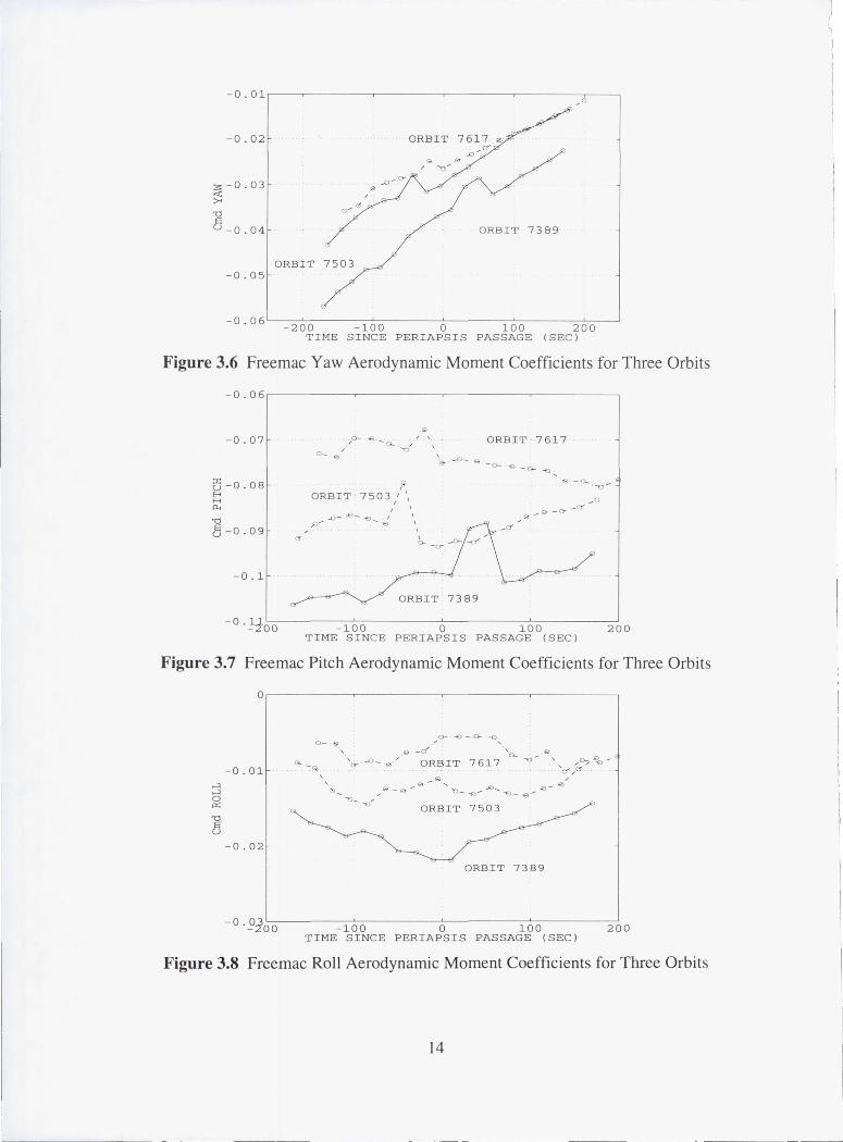
estimated at twenty second intervals. Figures 3.6, 3.7, and 3.8 show yaw, pitch, and roll
aerodynamic moment coefficients, respectively, for orbits #7389, #7503, and #7617 .
These estimates vary as the result of changing spacecraft attitude relative to the wind
velocity vector.
13
J
-o . o1 .---,---------r--------r--------~------~--~
-0.02 ORBIT 7617 0 -_rr
£> "
3:- 0 . 03
~ '0
(L o . 04 ORBIT 7389
ORBIT 7503 -0.05
-0.06~---2~0-0~-------1~0~0--------0~-------1~0-0--------2~0-0---"
TIME SINCE PERIAPSIS PASSAGE (SEC)
Figure 3.6 Freemac Yaw Aerodynamic Moment Coefficients for Three Orbits
-0.06 r-----------r-----------r-----------r---------~
-0.07 (OJ
/~ ~ -0.. / ( \
0 _ e / --0
ORBIT - 7617 , e -0_ e -0- €> -0- ~
is -0 . 08 E-o
;< ORBIT 7503 " " H _ 0
0.. I \
'0 0 -0 . 09
p _ ..o- ~- ~- .e: 13 _9- _ 13" - (f
-0.1
ORBIT 7389
-0·!±0~0~--------~1~0~0----------0~--------~1~0~0---------2~00 TIME SINCE PERIAPSIS PASSAGE (SEC)
Figure 3.7 Freemac Pitch Aerodynamic Moment Coefficients for Three Orbits
..:l
..:l 0 <>: '0
0
O r----------r----------~---------r--------_.
0 - &l
-0.01 , ..0
( y - e
- 0.02
0- -E> - 0- -0 , , " - if
ORBIT 7617 ,
"0_ "'E)_.JC) - 'E} _ e - SlJ- -0
ORBIT 7503
ORBIT 73B9
-0·~]OLO~--------~1~0~0----------0~--------~1~0~0--------~2~00 TIME SINCE PERIAPSIS PASSAGE (SEC)
Figure 3.8 Freemac Roll Aerodynamic Moment Coefficients for Three Orbits
14

Atmospheric parameterization is categorized into two types. In the first case,
VIRA scale heights and pitch moment coefficients (Figures 3.4 and 3.5) are assumed
correct. Base density and the remaining two aerodynamic moment coefficients are the
three parameters estimated. This method of atmospheric analysis will be referred to as
the "base density method." For the second approach, five parameters are used. These
five parameters are two scale height correction factors, base density, and the yaw and roll
aerodynamic moment coefficients. This technique will be called the "scale height
method." The scale height method can only be implemented when the pitch moment
coefficient is known throughout periapsis passage as shown in Figure 3.7. Also, the
spacecraft must experience a large amount of aerodynamic torque in order to successfully
measure scale height variation. Such torques are experienced only between orbits #7389
and #7626, therefore, scale height investigation is limited to these orbits. The base
density method can be applied to any orbit in Cycle Four.
III.3 Gravity Gradient Torques
Since the gravity field of Venus is not uniform (i.e., gravity follows an inverse-
square law), different locations of the spacecraft experience different levels of
gravitational attraction toward Venus. The result of this imbalance of forces is a net
external torque. It can been shown that a spherical gravity potential is sufficient to
accurately model torques due to gravity gradients at Venus. Assuming a spherical
potential, torques experienced due to the imbalance of gravitational forces, or gravity
gradients, are determined to first order by the equation _3
{[mn(l_z - l,y)+l(n 1_ -m l,: )+(n 2 -m 2 )I_,_ ]1
[+[lm(l -Ix,)+n(ml_-ll,_)+(m 2-12)I ]/_J
(5)
15

This equation uses moments of inertia and direction cosines to determine gravity
gradient torque. The direction cosines, l, m, and n, are defined by the position of Venus
in the Magellan spacecraft coordinate system shown in Figure I. 1. The distance between
the spacecraft and the planet, R, as well as the gravitational constant, It, are also known.
The only remaining values are the mass moments of inertia, which will be considered
unknown. Eq. (5) does not represent a set of independent measurements for the mass
moments of inertia. Note that the moments of inertia, Ixx, Iyy, and Izz, only appear within
Eq. (5) as differences. Accordingly, it is not possible to solve for all three moments of
inertia, Ixx, Iyy, and 1,1, using the gravity gradient equation. To overcome this problem, Ixx
was assumed to be known as the calibrated value 1106 kg.m< Ixxwas chosen since it is
not affected by solar array orientation. Change in Ixxdue to propellant mass loss was
assumed negligible due to the proximity of the fuel storage tank to the spacecraft yaw
axis and the small quantity of fuel used throughout the cycle. Fuel use during Cycle Four
caused a change in total spacecraft mass of only 0.04%.
The five parameters to model gravity gradient torque are therefore the five mass
moments of inertia: Iyy, Izz, Ixy, Iyz, I_z.
Figure 3.9 represents typical changes in reaction wheel speed due to gravity
gradient torques.
10
v
0
u]
,.-]-5
z_ -10
Figure 3.9
i/
i
ti
i
J, ROLL
t
YAW
........... _PITCH
_ e
_i 0J00 '-500 0 500TIME SINCE FERIAPSIS PASSAGE
)0 10h00 1500
(SEC)
Reaction Wheel Speed Due to Gravity Gradient Torque
16

III.4 Solar Pressure Torques
The final significant contribution to environmental torque is that due to solar
pressure. Solar pressure is the result of solar electromagnetic radiation interacting with
the spacecraft surface. Similar to the phenomenon associated with atmospheric pressure,
there exists some offset between center of solar pressure and spacecraft center of mass.
The result is an external torque which is modeled by the equation
=-cm p L,. (6)
Eq (6) applies to each of the three body-fixed axes. Mean solar momentum flux is
represented by p, while A_ and L are respectively, characteristic area (23 m 2) and length
(3.66 m). These three values are considered known leaving the solar moment coefficients
c,,_ as the only unknowns. One solar moment coefficient exists for each of the three axes.
As the spacecraft is inertially fixed, any solar moment coefficient is essentially
constant over the course of any single orbit. Further, momentum flux does not vary
significantly over the periapsis event. Consequently, torque due to solar pressure is
constant as long as the sun is visible to the spacecraft. Figure 3.10 shows change in
reaction wheel speed due to solar pressure. In this example, there is no change in reaction
wheel speed over some time interval near periapsis as the spacecraft passes through the
Venus shadow.
17

fa__q
ta,
ZO
,<r.x]r_
1.4
1.2
1
0.8
0.6
0.4
0.2
0
0-[{00 i000
TIME
Figure 3.10
, PITCH _ 7
-500 0 500 i000 1500
SINCE PERIAPSIS PASSAGE (SEC)
Reaction Wheel Speed Due to Solar Pressure Torque
Three parameters are required in order to model solar pressure torque. These parameters
are solar moment coefficients corresponding to the yaw, pitch, and roll directions.
III.5 Neglected Torques
Although only atmospheric, gravity gradient, and solar pressure torques are
modeled, other environmental torques may exist. Possible causes for these remaining
torques are magnetic field interaction and mass discharge. Since Venus does not have an
intense magnetic field, magnetic torque is estimated to be on the order of 1.10 -_°N.m.
This torque is neglected since it is nearly six orders of magnitude less than any of the
modeled torques. A mass discharge such as a fuel leak would result in a fairly constant
torque. This type of torque would be difficult to notice since it would appear as merely
additional solar torque. However, solar occultation could be used to distinguish torque
caused by solar pressure from that caused by mass discharge. During occultation, there
can be no solar pressure, however, torques caused by mass discharge would continue.
Also, mass discharge, such as a fuel leak, would result in an eventually noticeable fuel
18

loss. Since no significant fuel loss was reported by Martin Marietta during Cycle Four, it
is assumed that no torque was caused by mass discharge.
III.6 Final Reaction Wheel Speed Model and Parameters
The total torque model is composed of the individual models described in sections
Ili.2, Ill.3, and 111.4, such that
T= T_ +Te +T_ (7)
Eq. (8) through Eq. (11) are used to represent atmospheric, gravity gradient, and solar
pressure torques as functions of model parameters. Atmospheric torque is parameterized
by two methods. The first, base density method, is given by
L = (8)
while the second, scale height method, is
L : Ta (Po, O_ento" O_exit" fred,yaw' fred,roll ) (9)
Gravity gradient parameterization is of the form
T_= Tg(l,,Iu,lxr,lxz,Iyz) (10)
and finally, solar pressure is
T s -_ T s (Crtt,.,yaw, fins,pitch, Cntv,roll ) (11)
19

Reaction wheel speed is then the result of the integration shown in Eq. (1). Three
additional parameters are used to represent biases for the yaw, pitch, and roll reaction
wheel speeds. A bias parameter represents the speed of a reaction wheel at the beginning
of the simulation, and is represented by the constant, C, in Eq. (1). When the base density
scheme is used, the model has a maximum of fourteen parameters. On the other hand, the
model has at most sixteen parameters for the scale height scheme. Although fourteen or
sixteen parameters may be estimated using the above models, it is not always necessary to
estimate all parameters. If only base density and aerodynamic moment coefficients are of
interest, then solar moment coefficient and the mass moment of inertia parameters may be
removed from the model without introduction of significant error.
The following figure shows sample reaction wheel speeds for the pitch direction
in order to show relative influence of the atmospheric, gravity gradient, and solar pressure
contributions.
10f.fl
r/)
v 5
ra
ta.tn 0
,-3
ZO
r)
-10
,.,.,
DASHED: ATMOSPHERIC
r
SOLID: SOLAR PRESSURE_
! z
i i
.... _ .... _ . >
• i
• i
I
DOT+DASHED: GRAVITY GRADIENT
_%'oo .....-iooo -5oo o soo 1ooo _5oo_ME si.c_ PERIA_SIS_ASSA_ECSEC_
Figure 3.11 Example Contributions to Pitch Reaction Wheel Speed
20

IV. DIFFERENTIAL CORRECTION
IV.1 Introduction
In order to determine model parameters that best approximate Magellan data, a
differential scheme is employed• The general differential correction equations (see
Appendix B) are given by
: A rl-'-' -l]-'[A.rF/'z_ [ . c A.+l-'x E.
2+ 1 = 2 + A2
(12)
where n is the iteration number, and the sensitivity matrix, A, is given by
Arl
3co
o3_ I _0_ ,:la_ aGt:l 1=1
aco ,:2 "'" aco ,:2,:2 _ P2 3P.
• . .
aco" _co
-- t=N n
13)
and the measurement and a priori covariance matrices are given respectively by,
[20o]-1 0 -.- 0 ox_
2 02 1 ..- 0 g_2 "'"F_=o_ . ". Fx= . : '- 0
2
0 0 0 0 0 o,,M
(14)
21

Oncealist of M parameters is specified, Eq. (12) is used to determine the correction to
these parameters that minimizes the sum of residuals squared between model and
observed data consistent with the a priori information.
IV.2 Parameters
A maximum of sixteen parameters are used to model reaction wheel speed.
Parameter selection for reaction wheel modeling is based upon data availability. The
following table shows data restrictions for all model parameters.
Reaction Wheel Speed Model Parameter Reaction Wheel Data Requirement
biases (3) no restrictions
base density (1) include + 400 seconds of periapsis
mass moments of inertia (5) include _+ 15-20 minutes of periapsis
solar moment coefficients (3) include _+ 15-20 minutes of periapsis
aerodynamic moment coefficients (2) include + 400 seconds of periapsis
scale height correction factors (2) include + 400 seconds of periapsis
high rate data
strong atmospheric signal
Table 4.1 Data Requirements for Model Parameters
For scale height correction factors, an atmospheric signal is considered strong if it
causes a change in reaction wheel speed of 25 rad/sec or more within one orbit. This
requires the spacecraft to be below a certain altitude at periapsis depending upon local
solar time. Mass moment of inertia and solar moment parameters require data for an
extended amount of time due to the low frequency nature of the corresponding torques.
22

IV.3 A Priori
In Eq. (12), a priori knowledge is represented by the estimate, 15.,, and the
covariance, F_. The a priori covariance was found to be necessary for convergence only
in the case of moment of inertia parameters. Convergence was defined by the iteration
when all parameter estimates deviated from the previous iteration's estimates by less than
a convergence tolerance. The moment of inertia a priori requirement is attributed to the
fact that, depending upon the direction cosines of Eq. (5), some of these parameters are
poorly determined on any given orbit. However, in order to prevent the a priori estimates
from influencing the actual estimates of moments of inertia, a priori estimates were
removed from Eq. (12). This is identical to setting the a priori estimate equal to the value
of the current parameter estimate. Thus, the a priori covariance matrix only acts as a
conditioning of the information matrix, A,_F_tA_. 14
IV.4 Iteration and Convergence
Although the conditioning method assures solution convergence, it dramatically
increases the number of iterations required for convergence. As a priori covariance
values are lowered, iterations required for convergence increase. Conversely, as a priori
covariance values are raised, the possibility of solution divergence increases. Therefore,
optimal a priori covariance values exist such that the number of iterations is kept low, but
all solutions still converge. These optimal a priori covariance values were found by trial
and error and are shown in Table 4.2. No a priori knowledge was used for any parameters
other than those representing mass moments of inertia.
23

Moment of Inertia
Iyy
Izz
hy
Ixz
Iyz
A Priori Standard
Deviation, cr (kg.m 2)
23
15
20
20
20
Table 4.2 Spacecraft Bus Moments of Inertia A Priori
Unless scale height correction is included in the parameter set, all partial
derivatives of Eq. (13) are independent of the model parameters. Iteration is therefore
required to minimize the sum of residuals squared only for solutions that include either
mass moments of inertia or scale height correction factors.
IV.5 Cramer-Rao Bounds
Cramer Rao bounds are used as formal estimates of accuracy associated with
model parameters._5 The accuracy estimates for all parameters is given by the diagonal
values of the inverse of the information matrix, A[F_A,,.
V. RESULTS
V.1 Introduction
The reaction wheel speed model described in section III and the differential
correction method outlined in section IV are used to estimate model parameters
throughout Cycle Four. The following plot shows a sample orbit simulation where model
reaction wheel speed is compared to observed data. The solution set for this example
includes three solar parameters, three atmospheric parameters, five moments of inertia,
24

andthreebiases.This figure demonstratesthetorquemodelan/i'_ffferentialcorreciion's
ability to simulatereactionwheelspeed.
c/)
i0
5
0
-5
'-_ -10
_n-15
-20
Z -25O
-30
_ -35
--1%oo -lO'OO -5;o 6 500TIME SINCE PERIAPSIS PASSAGE
YAW
_rW2_l,_; _ " '" I....
PITCH ' ' • " ' _ '0 _ ,
DASHED : OBSERVED DATA
SOLID: MODEL MAY 23 , 1993
i000 1500
(SEC)
Figure 5.1 Reaction Wheel Speeds for Orbit # 7610
V.2 Atmospheric / Aerodynamic Parameters
The method used to parameterize the torque model for atmospheric and
aerodynamic contribution to reaction wheel speed dictates the type of results. Recall that
the base density method determines a base density and two aerodynamic moment
coefficients. For this method, all solutions are based upon the use of VIRA scale heights.
No scale height information is recovered from the base density method, however, it may
be applied to all of the orbits of Cycle Four. On the other hand, the scale height method
recovers base density, two scale height correction factors, and two moment coefficients.
The scale height method requires a strong atmospheric signal which is only present for
the final 250 orbits of Cycle Four.
25

V.2.1 Base Density Method
Base density method is the first method of parameterizing the atmospheric torque
contribution of the reaction wheel speed model. Atmospheric torque parameters are base
density and two aerodynamic moment coefficients. All results require the use of one
previously determined moment coefficient and known VIRA scale heights. The pitch
aerodynamic moment coefficients are estimated by free molecular flow simulations.
Once this value is assumed known, yaw and roll moment coefficients as well as base
density are estimated. The base density method was successfully used on 914 orbits in
Cycle Four. Parameters for all orbits were not recoverable for reasons related to limited
data coverage. However, for all orbits in which all required information was available,
parameter estimates were determined.
V.2.1.1 Base Density
Base density represents atmospheric density at some altitude below spacecraft
periapsis altitude. All densities above that altitude are determined from scale heights as
shown in Eq. (3). During the time period of this study, spacecraft altitude at periapsis
ranges approximately from 165 to 185 km. Base densities are expressed at 165 km for
consistency for all of Cycle Four. The following graph compares base densities as found
by the reaction wheel method to densities found by the orbital decay technique. _6 The
orbital decay method is an independent method of determining base density. For clarity,
atmospheric densities determined by orbital decay in Figure 5.2 are multiplied by a factor
of ten. This figure shows general agreement of base densities derived from the two
independent methods. A dramatic decrease in density occurs during the nighttime. Also,
measurements during the nighttime indicate a much larger degree of variability than the
daytime.
26

§;! -1.1 ...... 10 >< E-< H U)
@ -12
0 10
r..:l U)
,c( ORBIT 5760 III -13
ORBIT 7620
10 5~AM------1~0--AM-----3~P-M----~8~P-M~--~1~AM------6~AM----~11 AM LOCAL SOLAR TIME
Figure 5.2 Density as Determined By Reaction Wheel Method and Drag Method
When compared on an extended time scale, many of the short term features
compare favorably including the "four day period" and nighttime variability. Figure 5.3
shows base densities from Figure 5.2 between 9 AM and 10 AM, early in Cycle Four.
U") \.()
M 1
~ >< E-< H U)
~ o r..:l ~ 0.5 III
9
DRAG METHOD: CIRCLE & D~TTED
REACTION WHEEL METHOD: CROSS & SOLID
o
9.2 9.4 9.6 9.8 LOCAL SOLAR TIME (AM)
10
Figure 5.3 Reaction Wheel and Drag Method Base Density Between 9 AM and 10 AM
27

L
Figure 5.3 shows agreement between base densities trends as determined by reaction
wheel data and drag data.
V.2.1.2 Yaw and Roll Aerodynamic Moment Coefficients
Just as the free molecular flow simulation estimates the pitch aerodynamic
moment coefficient, it also estimates the yaw and roll coefficients. These moment
coefficients are not used at any time in the base density parameterization method. This
provides the opportunity to independently verify consistency between the Freemac
moment coefficients. The yaw aerodynamic moment coefficients as estimated by the
base density method are shown compared to Freemac values in Figure 5.4.
0.1 .-----~----------~----------~----------.--.
". t o
CIRCLES: F REEMAC FLOW'SIMULATIO
-0 .1
POINTS : REACT ION WHEEL METHOD
6000 6500 7 000 7500 ORBIT NUMBER
Figure 5.4 Yaw Aerodynamic Moment Coefficient
The yaw moment coefficient shows close agreement between the reaction wheel and the
Freemac estimate between orbits #5800 and #6600, as well as between #7250 and #7620.
These orbits correspond to daytime local solar hours. During the nighttime, density is
considerably lower, making aerodynamic moment measurement more difficult.
28

Theroll aerodynamic moment coefficients as estimated by the base density
method is shown compared to Freemac values in Figures 5.5.
0.04
0.02,-IO
? o
-0 . 02
-0. 04
• • _ ' .0
-:.-......'. :• ": ...,.. ..._:"-."
".t% : . .
• " . -. _.°. m_" :° -.
: : • _. ° :. ". °t. :
: : °.° _" . . :
_ . ....'...,-._:_.:::._-...'_....... _ . . \ ., ,_ •
_.: : ....:: ............. i........................ ..................CIRCLES: FREW.MAC FLOW SIMULATION :
POINTS: REACTION WHEEL METHOD
I I
60'00 6500 7000 75a00
ORBIT NUMBER
Figure 5.5 Roll Aerodynamic Moment Coefficient
As with the yaw moment coefficient, a large discrepancy appears between orbits #6600
and #7250, for the roll moment coefficient. Again, these orbits occur during the
nighttime hours when density is much lower. Also, Freemac estimates of the roll moment
are consistently high early in Cycle Four, and are likewise consistently low late in the
cycle. This offset could be due to a center of mass located in a different location than
assumed by the Freemac model. Current Freemac simulations place the center of mass
location on the positive roll axis, 6.259 inches from the yaw-pitch plane. If the offset
shown in Figure 5.5 is due to error in spacecraft center of mass location, the sign of this
offset indicates that the center of mass is actually above the pitch-roll plane. This is the
side of the spacecraft with the altimeter antenna (see Figure 1.1).
Other possible explanations for this disagreement are accommodation
coefficients, and solar array position errors within the Freemac model. Momentum and
thermal accommodation coefficients are used to characterize the nature the interaction of
29

anatmosphericparticleandthespacecraftsurface.The coefficients dictate the amount of
energy and momentum absorbed by the spacecraft. Errors in these coefficients may cause
significant error in aerodynamic moment coefficients. Errors in positions of the solar
arrays may also affect aerodynamic moment coefficients. Solar array position has an
uncertainty of_+ 0.5 degrees under nominal conditions, however, this error may increase
dramatically during occultation. During this time, sun-sensors are unable to track the sun
and solar array position error may increase to 11 °. This error is caused by non-linear
effects of solar array position potentiometers (Personal communication, M. Patterson,
Martin Marietta Corporation, March 10, 1994). This error should only appear during
occultation which corresponds approximately to orbits #6600 through #7200. This type
of solar array position error can therefore not be responsible for the roll offset shown in
Figure 5.5 during late and early Cycle Four.
V.2.2 Scale Height Method
The second method of parameterizing the atmospheric torque model allows the
examination of scale heights in addition to base density. In this case, the method
estimates a base density, two scale height correction factors, and the yaw and roll
aerodynamic moment coefficients. The base density again represents density at some
base altitude below the altitude of spacecraft periapsis. Densities above that altitude are
determined from Eq. (4). Scale height correction factors, t_, are used to modify VIRA
scale heights. Whereas the base density method needs only one constant pitch moment
value from Freemac, the scale height method requires that pitch moment coefficients be
known throughout the orbit. The yaw and roll moment coefficients are estimated as
single, constant values for a given orbit. If the Freemac yaw and roll moment coefficients
are consistent with the pitch coefficient, it would be expected that the scale height method
estimates should be approximate averages of the Freemac estimates.
30

Base densities recovered using the scale height method will vary slightly from the
solutions from the base density method. However, these solutions only vary due to the
change in scale heights. Accordingly, base density estimates recovered using this method
are not shown.
V.2.2.1 Scale Heights
Two scale height correction factors are determined for each orbit. The first
represents deviation from VIRA scale heights within the atmospheric entry portion of the
orbit (in), while the second ;epresents the exit of the atmosphere (out). The entry portion
of the orbit corresponds approximately to a region from 19 ° to 11° north latitude.
Similarly, the exit portion occurs from 11 ° to 3 ° north latitude. Scale height correction
factors are used to calculate modified scale heights.
Figures 5.6 and 5.7 demonstrate the ability of reaction wheel data to recover
information related to spatial variation in atmospheric density. This graph represents
example residuals before and after applying the scale height correction factors. A spline
filter is used to smooth residuals for purposes of presentation. When VIRA scale heights
are used rather than modified scale heights, the differential correction algorithm is unable
to fit the observed data to the noise level, i.e., some type of signal appears within the
residuals. This signal is shown by the dashed lines of Figures 5.6 and 5.7. However,
scale heights can be modified such that this signal is removed from the residuals. Scale
heights are modified by multiplying each scale height by the appropriate scale height
correction parameter, _. In these two figures, solid lines represent residuals after using
modified scale heights. Essentially all signal is thus removed from the residuals and scale
height information is recovered.
31

2 _
ALPHA IN = 1.13 ALPHA OUT = 0.88
1.5- .........
_ i..............._ ......................................................h
v 0 . 5 i _ ....... ............... .............. ....................
u) f i -
n. 1 5_ SOLID LINE: AFTER SCALE HEIGHT CORRECTION 1
IDASHEDL_NE'._EFORESC_._.HEIGHTCORRECTIONI-_o -16o _ i_o 2_o
•_.E S_NCE_ERI_S_S PASSAGECS_C)
Figure 5.6 Scale Height Correction Effect on Residuals of Orbit #7511
21" ALPHA IN : 1.18 ALPHA. OUT= i i__.5_" ........ ........... ........ ......
_ _I'.......................................................:.......................o.5 ...............A..............A......;..,,.,',,.........;..............
_ 0 _ r__'i*, ........... _..........
-o.5 , ,, '' ,",;i ...................! r 11
-1 , r ............ ..................
I_CA_ HEIGHT CORRECTION_oo i i i
-i00 0 i00 200TIME SINCE PERIAPSIS PASSAGE (SEC)
Figure 5.7 Scale Height Correction Effect on Residuals of Orbit #7479
Scale height determination was completed for approximately 150 orbits late in Cycle
Four. As stated above, scale height determination requires Freemac estimates of the pitch
moment coefficient as it varies through the orbit. These pitch moment coefficients,
shown in Figures 3.6, 3.7, and 3.8, are available for orbits #7389, #7503, and #7617. For
orbits that the aerodynamic coefficients are not available, the nearest orbit's estimates are
used. These coefficients are estimated at twenty second intervals throughout the
atmospheric event. A linear interpolation is used to determine pitch moment coefficients
at times within these twenty second intervals.
32
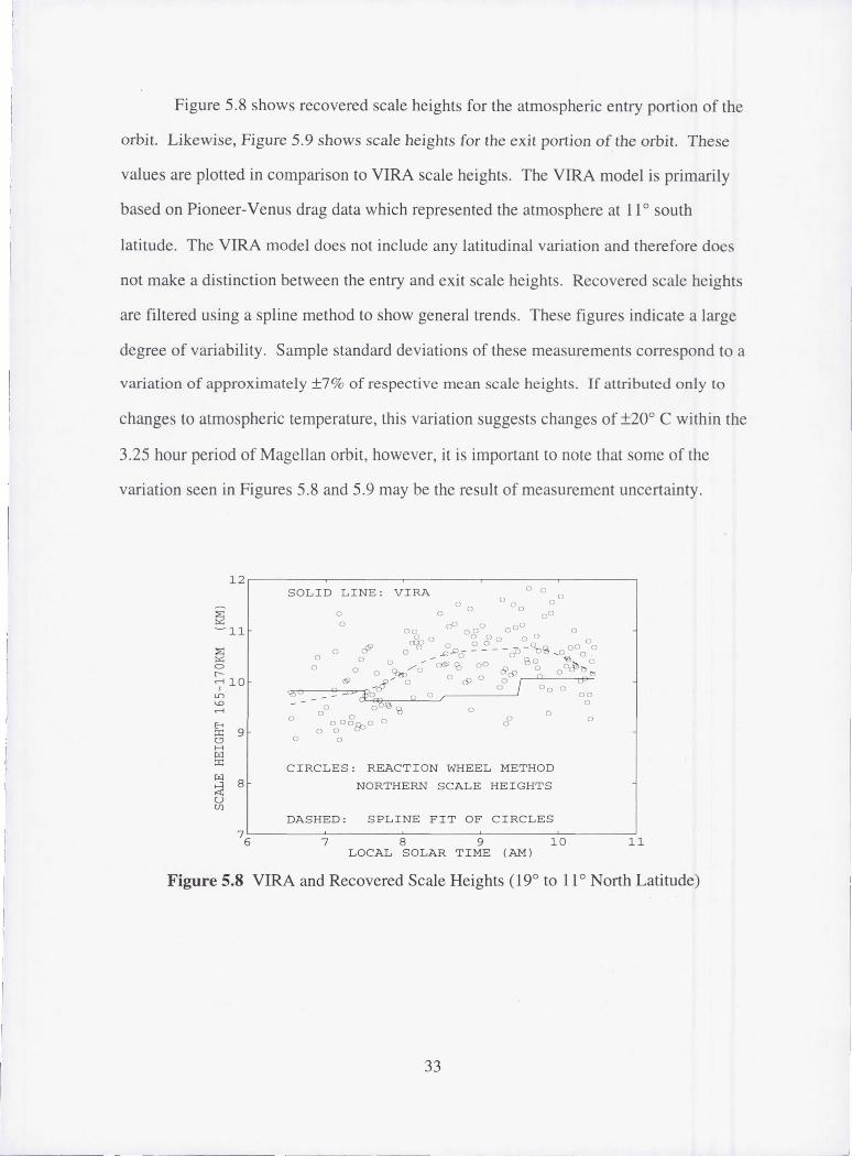
Figure 5.8 shows recovered scale heights for the atmospheric entry portion of the
orbit. Likewise, Figure 5.9 shows scale heights for the exit portion of the orbit. These
values are plotted in comparison to VIRA scale heights. The VIRA model is primarily
based on Pioneer-Venus drag data which represented the atmosphere at 11 0 south
latitude. The VIRA model does not include any latitudinal variation and therefore does
not make a distinction between the entry and exit scale heights. Recovered scale heights
are filtered using a spline method to show general trends. These figures indicate a large
degree of variability. Sample standard deviations of these measurements correspond to a
variation of approximately ±7% of respective mean scale heights. If attributed only to
changes to atmospheric temperature, this variation suggests changes of ±20° C within the
3.25 hour period of Magellan orbit, however, it is important to note that some of the
variation seen in Figures 5.8 and 5.9 may be the result of measurement uncertainty.
12.-------~-------.--------._------~------__,
Q o e-,...; 10
I L()
'D ,...;
~ 9 c.'J H r.LI ::r:
~ 8 u U)
CIRCLES: REACTION WHEEL METHOD
NORTHERN SCALE HEIGHTS
DASHED: SPLINE FIT OF CIRCLES 76L-------~7~------~8~------~9------~1~0~----~11
LOCAL SOLAR TIME (AM)
Figure 5.8 VIRA and Recovered Scale Heights (190 to 11 0 North Latitude)
33
12r-------~------~--------~------~------__.
~ ~11
~ o e-n 10
I L.()
\.D n
SOLID LINE: VIRA
o o
o o o o
~ 8 CIRCLES: REACTION WHEEL METHOD .:x: ~ SOUTHERN SCALE HEIGHTS
DASHED: S PLINE FIT OF CIRCLES
7 8 9 1 0 LOCAL S OLAR TIME (AM)
11
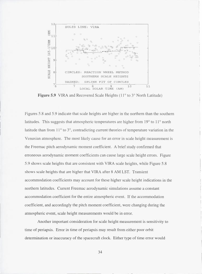
Figure 5.9 VIRA and Recovered Scale Heights (11 ° to 3° North Latitude)
Figures 5.8 and 5.9 indicate that scale heights are higher in the northern than the southern
latitudes. This suggests that atmospheric temperatures are higher from 19° to 11 ° north
latitude than from 11 ° to 3°, contradicting current theories of temperature variation in the
Venusian atmosphere. The most likely cause for an error in scale height measurement is
the Freemac pitch aerodynamic moment coefficient. A brief study confirmed that
erroneous aerodynamic moment coefficients can cause large scale height errors. Figure
5.9 shows scale heights that are consistent with VIRA scale heights, while Figure 5.8
shows scale heights that are higher that VIRA after 8 AM LST. Transient
accommodation coefficients may account for these higher scale height indications in the
northern latitudes. Current Freemac aerodynamic simulations assume a constant
accommodation coefficient for the entire atmospheric event. If the accommodation
coefficient, and accordingly the pitch moment coefficient, were changing during the
atmospheric event, scale height measurements would be in error.
Another important consideration for scale height measurement is sensitivity to
time of periapsis. Error in time of periapsis may result from either poor orbit
determination or inaccuracy of the spacecraft clock. Either type of time error would
34
---------- -------.--- ~ ~ - - ----

result in an atmospheric torque anomaly similar to that of scale height error. For this
reason, scale height measurements are now examined as a function of time of periapsis
error.
Figure 5.10 shows scale height correction factor, as error is introduced to time of
periapsis.
~ 5,---------~--------.---------~------__. E-<
~ 4' ~, DASHED LI NE: . S OUTHERN CORRECTION ·
5=: 3 <..? H
gj 2
~ l
cJ U) 0 Z H - l Iil CJ ~ -2
u -3
~ -4
~
. '
SOLID LINE : NORTHERN CORRECTI ON
~-~2L----------l~--------O~--------~l--------~2
TIME OF PERIAPSIS ERROR ( SEC)
Figure 5.10 Scale Height Correction Factor Sensitivity to Time of Periapsis Error
The first is uncertainty associated with the spacecraft clock, however, this error is
small since the onboard clock is calibrated to 8 milliseconds of Universal Time. 17 Error
may also be introduced by the orbit determination. Time of periapsis as determined by
Doppler data is considered to be known better than 0.1 seconds for the Magellan orbit late
in Cycle Four (Personal communication, Kuen Wong, Jet Propulsion Laboratory, March
29,1994). Figure 5.10 indicates that this error is acceptable for scale height
measurements.
35

--- --- - --
V.2.2.2 Yaw and Roll Aerodynamic Moment Coefficients
Yaw and roll aerodynamic moment coefficients are also determined by the scale
height method. Although Freemac estimates moment coefficients for attitudes near
periapsis, this reaction wheel method only estimates two constant coefficients, i.e., one
coefficient for each direction. These two estimates represent the average aerodynamic
yaw and roll moment coefficients during the atmospheric event. As in the case of the
base density method, the yaw and roll moment coefficient can be compared with Freemac
estimates to evaluate consistency. Figure 5.11 shows yaw moment coefficient as
determined by Freemac compared to the estimate by the scale height method. The
reaction wheel derived estimate appears to be close to the average value of the Freemac
estimate, therefore confirming consistency between the yaw and pitch moment
coefficient.
~
- O_Ol,--~---~------~------~----~--.
-0.02
SOLID LINE: REACTION WHEEL ESTIMATE
Q "
/
"
~ -0.03
-0.04
DASHED LINE : FREEMAC ESTIMATE
- 0 _ 05L--_2~0~0~----_ ~lO~0~----~0------~l70~0--~2~0~0~ TIME SINCE PERIAPSIS PASSAGE (SEC)
Figure 5.11 Yaw Aerodynamic Moment Coefficient for Orbit #7503
Likewise, the roll aerodynamic coefficient as estimated by reaction wheel data is
compared to the Freemac estimate in Figure 5.12. This figure shows the same type of
inconsistency that was indicated by the base density method shown in Figure 5.5.
36
1

,--------
l I I I
...:l
...:l o
O,-~~----~------~-------.------~--~
0::: -0.01
~
DASHED LINE: FREEMAC ESTIMATE
SOLID LINE: REACTION WHEEL ESTIMATE
-O.02L--~2~O~O~---_~1~O~O------~O-------1~O-O------20~O--~ TIME SINCE PERIAPSIS PASSAGE (SEC)
Figure 5.12 Roll Aerodynamic Moment Coefficient for Obit #7503
V.3 Mass Moments of Inertia
Since Ixx was assumed to be known in all solutions, only five moments of inertia
were determined. Changes in moments of inertia during Cycle Four can be attributed to
movement of the solar arrays. By knowing solar array position and mass distribution
(Personal communication, H. Curtis, Martin Marietta Corporation, June 4, 1993) of the
solar arrays, a theoretical model of moment of inertia variation was developed (see
Appendix C). The solar arrays were modeled as thin plates of mass 35 kg, based on
preflight properties. This solar array model contributes to total spacecraft moments
through Ixx = 37 kg·m2, Ixy = Ixz = O. The remaining moments of inertia are functions of
the solar array position. Total moments of inertia, as used by Eg. (5), can then be
determined as the sum of moments of inertia of the Magellan spacecraft bus and the solar
arrays. The differential correction algorithm was designed to estimate values of
spacecraft bus moments of inertia. Figures 5.13 through 5.20 show modeled moments of
inertia of the solar arrays and estimates of the spacecraft bus moments of inertia.
Discontinuities appear in the solar array moment of inertia curves due to solar array off
point adjustments. Moments of inertia are not determined between orbit #5938 and orbit
37

#6462 due to limited data coverage. Figures of solar array model moments of inertia are
headed by the model equation as derived in Appendix C. Figures of estimated bus
moments of inertia also contain error bars indicating measurement mean and standard
deviation.
86o.-------~------~------~------~----__,
855
850
_845 N < ::>: 840 ... CJ
=835
~830
H 825
820
815
---.~
/
8~~~0~0----~6~0~0~0----~6~5~0~0~--~7~0~0~0~--~7~5~0~0~--~8000 ORBIT NUMBER
Figure 5.13 Model Mass Moment of Inertia Iyy of Magellan Solar Arrays
1200
1195
1190
1185 N
1 ~ 1180 ... CJ =1175
~1170
H 1165
1160
1155
11~~00 6000 6500 7000 ORBIT NUMBER
, . ': ',.
7500 8000
Figure 5.14 Estimated Mass Moment of Inertia Iyy of Spacecraft Bus
38
_ J

As shownin Table4.2,thea priori standarddeviationusedfor Iyy is 23 kg.m 2. All
estimates of Iyyclearly lie within _+23 kg.m 2 of the estimated mean. Therefore, estimates
are considered not to be restricted by the a priori covariance. Some correlation exists
between the solar array model and spacecraft bus estimates of Iyy, probably due to a slight
error in the solar array model•
l_z =813+37sin2_ (kg.m 2)
860
855
850
_845
840<.9
_835
83ONNH 825
82O
815
8 %'oo 60'00 65'00 70'00 75'00 8000
ORBIT NUMBER
Figure 5.15 Model Mass Moment of Inertia Izz of Magellan Solar Arrays
750
745
740
735
g,'73o,_ I_725
N 720N
HTI 5
710
705
".z--&'_.. _ %. :-::.
i--- - -.
• -
7%%'00 60'00 6500 70'00 75'00 8000
ORBIT NUMBER
Figure 5.16 Estimated Mass Moment of Inertia Izz of Spacecraft Bus
39

For the estimate of spacecraft bus I_, Table 4.2 indicates an a priori standard deviation of
15 kg.m 2. Figure 5.16 shows this parameter not to be restricted by the a priori covariance.
A positive correlation exits between the solar array and bus 1,1 values before the
conjunction roll maneuver (orbit #7164) and a negative correlation exits afterwards. This
again suggests a small error in the solar array moment of inertia model.
Iy z = 19sin2_ (kg.m z)
25
2O
15
10
5¢.9
0
-5
H -i0
-15
-2O
/
%%00 60'oo 7000 75'00 800065'00
ORBIT NUMBER
Figure 5.17 Model Mass Product of Inertia Iyz of Magellan Solar Arrays
25
20
15
i0
cq
,k
-15
-2O
-%%'oo
Figure 5.18
l . . -_i.:'"•
t
6000 65_00 70'00 75'00 8000
ORBIT NUMBER
Estimated Mass Product of Inertia Iy z of Spacecraft Bus
40

A priori standard deviation for Iyz is 20 kg.m 2. Estimates are not restricted by this a priori
information. No correlation is apparent between the estimated spacecraft bus and
modeled solar array lyz.
3O
151
4,
N 5
oH
-5
-10
-15
• . , -- . . .' . ... -,
; . "'"- .. l -f, " . T
..... -j t-.,.¢,.'..:...."., , /# f D i.... :. - _._o-,_." _.:, _..o."_:.
•/': , • • " " :,i::7"-"',"• " ]_/
000 o5o0 ?000 75'oo 80o0
Figure 5.19
ORBIT NUMBER
Estimated Mass Product of Inemia Ixy of Spacecraft Bus
6O
55
5O
_450
_4o --
N35X
H
3O
25
{%o0
Figure 5.20
: e'"
i .'- .- -.. ." ;
":. . ." .. -- .:.:,. ,:'.._ • . "; - .:. :
_'." . "'" .'...;:';:.'". .. : v-:,_:" , - . _:-,_... .
6000 6500 7000 75'00 8000
ORBIT NUMBER
Estimated Mass Product of Inertia Ix, of Spacecraft Bus
Modeled solar array moments of inertia Ixy and Ix, are not shown since they are
identically zero. A priori standard deviations for I,y and Ixz are both 20 kg-m 2. Figures
41

5.19and5.20showtheseestimatesarenotrestrictedby theapriori. Thesetwo figures
alsoshownosignificanttrendsindicatingsolararraymomentof inertiacorrelation.
Meanvaluesandstandarddeviationsof theestimatedmomentsof inertia from
Figures5.14,5.16,5.18,5.19,and5.20,areshownin Table5.1.
Moment/Product Mean StandardDeviationof Inertia (kg.m2) (kg.m 2)
Iyy 1176.4 7.0
Lz 725,3 4.8
I_y 2.0 5.3
I_z 41.0 7.1
Iyz -3.9 6.5
Table 5.1 Spacecraft Bus Mean Estimated Moments of Inertia
Total moments of inertia were determined by adding bus and solar array moments
of inertia. Maximum and minimum values occur when the solar arrays pass through
either the spacecraft XY or XZ plane as shown in Table 5.2. I_ is highlighted to indicate
that it is not an estimated parameter. Mass moment of inertia values as estimated by an
in-flight calibration performed by Martin Marietta are also included in Table 5.2.
Moment/Product
of InertiaSolar Array in
XY Plane (kg.m 2)
Reaction Wheel
Method Estimate
Solar Array in
XY Phme (kg.m 2)
Martin Marietta
Calibration
Solar Array in XZ
Plane (kg-m 2)
Reaction Wheel
Method Estimate
Lx 1106 1106 1106
Iyy 1989.1 ...... 1975 2026.4
L_ 1575.3 1577 1538.0
hy 2.0 2.55 2.0
lx_ 41.0 37.4 41.0
Iy_ -3.9 1,1 -3.9
Table 5.2 Magellan Spacecraft Total Moments of Inertia
42

V.4 Solar Pressure Moment Coefficients
Solar parameters were determined for Cycle Four in the form of c,_,. These
parameters were not determined before orbit #6462 due to limited data coverage. One
such parameter exists for each coordinate axis; yaw, pitch, and roll. Solar moment
coefficients are plotted as a function of solar longitude. This Solar longitude is defined
within the spacecraft coordinate system as the angle between the roll axis and the sun-
vector projected into the pitch-roll plane. Solar latitude is then defined by the elevation
of the sun-vector above the pitch-roll plane. Figure 5.21 shows the solar longitude and
latitude definition
Yaw
Sun
Pitch
Figure 5.21
Latitude
I
[
Roll
Solar Longitude and Latitude Definition
Figure 5.22 shows solar longitude and latitude for Cycle Four. The solar latitude is near
-10 ° for much of Cycle Four due to the 10° Earth-point roll (see Appendix E, Figure
E. 15).
43

3O
25
20f.,.]r_
£.9 15
10
r_
C_ 5
5
_ _5 i-10
15
-2_5' 0 8L0 _ , _ 'I00 120 1 0 160
SOLAR LONGITUDE (DEGREES)
180
Figure 5.22 Cycle Four Solar Longitude and Latitude
Since the spacecraft rolls 180 ° prior to conjunction, solar longitude never increases above
180 °. Thus, the same side of the spacecraft always faces the sun. Solar longitude starts at
approximately 70" and proceeds toward 180 ° as the sun appears to rotate about the
spacecraft. After conjunction and completion of the spacecraft roll maneuver, the solar
longitude returns toward 70 ° . Large values of solar latitude near conjunction result from
the rolling spacecraft.
Figures 5.23, 5.24, 5.25, show c,,,, for Cycle Four. In these figures, circles
represent orbits prior to conjunction and crosses represent orbits after conjunction.
44

>._
¢..)
0 . l-
SOLID LINE: SPLINE
Oo •
..... ,, _ "_+ "_o__o_<:<.
CIRCLE: BEFORE CONJUNCTION
CROSS: AFTER CONJUNCTION
8'0 160 120 140 160 180
SOLAR LONGITUDE (DEGREES)
Estimated Yaw Solar Moment Coefficient for Cycle Four
The yaw solar moment coefficient shows a clear minimum when solar longitude is 90 °. It
also approaches zero as solar longitude approaches 180 °. The maximum yaw moment
coefficient corresponds to a solar longitude of 145 °. Solar torque in the yaw direction is
largely the result of the High Gain Antenna (HGA). At 90 ° the cross sectional area
presented to the sun by the HGA is a minimum, thus causing the minimum moment
coefficient. At 180 ° the HGA shows a large cross section for solar pressure, but the net
force acts through the yaw axis, thus causing no torque. A maximum occurs somewhere
between 90 ° and 180 ° where the HGA causes the largest product of cross sectional area
and moment arm. This corresponds to 145 ° according to Figure 5.22. The symmetric
nature of the spacecraft should cause the yaw moment coefficient to be symmetric about
the solar longitude angle 90 ° , such that another maximum would occur at 35 ° solar
longitude and another zero at 0 ° solar longitude.
Estimates of the yaw moment coefficient appear to have slightly different values
before and after conjunction, but still follow the same trends.
45

Figure 5.23 shows a yaw moment coefficient that is not exactly zero at a solar
longitude of 180 °. This is most likely explained by "shadowing" effects of the solar
arrays caused by the high solar latitude shown in Figure 5.22.
0.i ' ! T ! '-
0.08 ...............................CIRCLE : BEFORE CONJUNCTION
0.06[ ............. .... o.......... ..................................... ......... ..
0.04, .... .... o ......... _ ............. :'_,_ "
e°°$° " " : " zP""-_'_"_'_/
-o.o,[.............. oo°,o°,,........... .......-o. o8 t-....... ........... .............. i_ ......... ; ........... i .........
/ CROSS: AFeER CONJUNCTZON-°'k'o 8'o 16o i .o i;o lao
SOLAR LONGITUDE (DEGREES)
Figure 5.24 Estimated Pitch Solar Moment Coefficient for Cycle Four
Figure 5.24 indicates that the largest torque in the pitch direction due to solar pressure
occurs when the solar longitude is between 170 ° and 180 ° . At this time, solar latitude
reaches its maximum value of 20 ° , as shown in Figure 5.20. This high solar latitude is
responsible for the high solar pitch moment coefficient. As expected, a zero in the pitch
coefficient occurs near a solar longitude of 160 ° when the latitude is also zero. The pitch
moment coefficient also approaches zero as solar longitude nears 90 ° . This is the result
of the net solar pressure force acting almost completely in the pitch direction. Under this
condition, little torque can be created about the pitch axis.
Figure 5.25 shows the roll solar moment coefficient. This figure indicates that the
roll direction experiences very little torque due to solar pressure.
46

0.02
o
_-0. 02
-0. 04
-0.06
-0.08
- 0. J6LO
Figure 5.25
0.i : _ !
0.08 -- CIRCLE: BEF'0RE CONJUNCTIoN .... o: ........
0.06 ......................................*......i................i.......................
0.0 ................ .,. ...... . ..................... :2 ..... i "• o: ° ° oo. ,) ° . .,_,
.......... i........... Z....... "_= °: _'_ .... _ °*:_ LL )* .... ! ...... #_F-o .boo o = *g_ _@ _o _o oO _ o° - .N
..........i.C.." ),° _ ......_ _f_, IP".,)W(r .o
: Z % • : • ° i
. ............ ......... °..! ....... - ...... _,........... ......... i ..........
CROSS : AFTER CONJUNCTIONi I I I I
80 i00 120 140 160 180
SOLAR LONGITUDE (DEGREES)
Estimated Roll Solar Moment Coefficient for Cycle Four
VI. ACCURACY ANALYSIS
VI.1 Introduction
An accuracy estimate for a given parameter is obtained directly from the
information matrix, ArF_IA,. Namely, Cramer-Rao bounds are used as indicators of the
accuracy of estimated parameters. The measurement covariance matrix, I-'_, is given by
2Eq. (14), where cr_ = 0.0827 rad 2 / sec 2. This value is derived from estimating the
standard deviation of a uniform distribution of values within the quantization error of the
reaction wheel tachometer. The definition of the measurement covariance matrix in Eq.
(14) assumes no correlation between successive data points. Such a correlation would
result in values for the off-diagonal terms of this matrix.
Accuracy estimates are also recovered by examining the statistics of estimates of
parameters that do not have a large degree of natural variability. Parameters such as
moment coefficients and mass moments of inertia should not vary significantly from orbit
47

to orbit. Standard deviations of these estimates thus provide a valid estimate of a
parameter's measurement "repeatability."
Determining the accuracy associated with mass moment of inertia parameters
using Cramer-Rao bounds, is complicated by the a priori requirements. For solutions
containing these parameters, conditioning the information matrix with a priori covariance
is necessary in order to determine the inverse. For this reason, accuracy of moment of
inertia parameters is estimated by statistical analysis of the final estimates only.
VI.2 Base Densities
Accuracy estimates for the base density and scale height method are essentially
the same. For this reason, error analysis is presented only for the base density method
since it represents the entirety of Cycle Four. Figure 6.1 shows normalized accuracy for
base density. In this case, the accuracy estimate is normalized by dividing by the base
density for the given orbit. Crosses are used to indicate orbits where high rate data was
available, while circles represent the low rate.
i00
_i0
o
[9
5q
'_0.i
Dfl
_xa
0.0
Figure 6.1
CROSS: HIGH RATE DATA × x x
X x Xx X
× _ x
o _ _ '1 x
.... x
CIRCLE: LOW RATE DATA
3' 8' i' 'AM i0 AM PM PM AM 6 AM ii AMLOCAL SOLAR TIME
Normalized Base Density Accuracy Estimate
48

Accuracydecreases dramatically during nighttime local solar times. During this period,
atmospheric base density is much lower than during the daytime. Accordingly, the
signal-to-noise ratio is significantly lowered, resulting in lower normalized accuracy.
During the daytime, accuracy are generally better than 0.5%. This is of course more
accurate than the pitch aerodynamic moment coefficient estimate by Freemac, therefore,
the limiting factor in determining base density from reaction wheel data is the pitch
moment coefficient. Near a local solar time of 10 AM, transmitted data went from the
high to the low rate. A noticeable decrease in accuracy occurs at this time, indicating the
method's sensitivity to data transmission rate. Cramer-Rao bounds indicate a
measurability threshold for density of 8 •10 -13 kg/m 3 for high rate data and 4 •10 -12 kg/m 3
for low rate data.
VI.3 Yaw and Roll Aerodynamic Moment Coefficients
Accuracy estimates for the yaw and roll moment coefficients are presented in a
different fashion than the base density. Aerodynamic moment coefficients may have
values very close to zero, making the normalized accuracy undefined. For this reason,
absolute accuracy estimates are shown for the yaw and roll moment coefficient as
determined by Cramer-Rao bounds. Figure 6.2 shows these values for the yaw moment
coefficient. Again, crosses indicate high rate and circles represent low rate data.
49

I°° r
101f 1o.I
10 3
_i0 -#
xCROSS: HIGH RATE DATA
CIRCLE: LOW RATE DATA
xXN X
x%aN _x
6000 65'00 70'00 75'00 8000
ORBIT NUMBER
Figure 6.2 Yaw Aerodynamic Moment Coefficient Accuracy Estimate
Again, accuracy decreases significantly after sunset, and then increases after sunrise.
After sunset, base densities drop making aerodynamic measurement more difficult. The
lower transmission rate also decreases the yaw moment coefficient accuracy. Cramer-
Rao bounds indicate a measurement threshold of 0.001 during the daytime.
Figure 6.3 shows the roll moment coefficient accuracy estimate.
i01
_1oH
10 -I
i0 -2
tJt3
I0 3
O
_i0 -4
No
-5
105500
x
xCROSS : HIGH RATE DA%IA
x xx
CIRCLE: LOW RATE DAT_ x
x x x x
60'00 65_00 7000 7500
ORBIT NUMBER8000
Figure 6.3 Roll Aerodynamic Moment Coefficient Accuracy Estimate
Figure 6.3 repeats the same trends as base density and the yaw moment coefficient for
local solar times and transmission rates. Measurement threshold for the roll aerodynamic
50

moment coefficient, as determined by Cramer-Rao bounds, is essentially the same as the
yaw moment coefficient.
In order to validate the Cramer-Rao error estimates for the yaw and roll
aerodynamic moment coefficients, the "scatter" of the actual measurements as shown in
Figures 5.4 and 5.5 is examined. Breaking the estimates into 38 groups of 24 orbits
allows for statistical analysis of the measurement. Each group of 24 orbits is used to
determine one sample mean and standard deviation. Figure 6.4 shows these sample
standard deviations.
10° .-----~------~------~------~------~
CROSS,SOLID: YAW
CIRCLE,DASHED:
I \ 0 \ ' 3
\
I, 0 C!> \
-4 105570~0----~670~00~--~65~0~0~--~7~0~0~0----~7~5~0~0----~a~000
ORBIT NUMBER
Figure 6.4 Yaw and Roll Aerodynamic Moment Coefficient Sample Standard Deviation
Figure 6.4 indicates a factor of ten lower sample accuracy during the daytime than
Figures 6.2 and 6.3. This disagreement indicates that the current error model is not
correct. One of the primary assumptions of the error model is that the data is a uniform
distribution within the measurement quantization. Close examination of the observed
reaction wheel speed as received from the telemetry stream reveals that the signal is not
always contained within the measurement quantization as explained in section IT.3. As
reaction wheel speed approaches zero, the measurements noise increases to as much as ±
51

i
L
2.5 rad/sec. A uniform distribution of ±2.5 produces a measurement covariance of
cr~ = 2.08 rad '1 / sec 2 • This is approximately 25 times larger than the covariance when
the data is assumed to stay within the measurement quantization. Estimated error from
Cramer-Rao bounds would have been five times larger if this large covariance was used.
As the reaction wheel increases speed, the measurements tend to return to within ± 0.5
rad/sec, but not until the reaction wheel achieves a speed of nearly 25 rad/sec. This
variation can be seen in the observed reaction wheel speed signal of Figure 5.1. The
measurement standard deviation is therefore a function of reaction wheel speed. A more
sophisticated error model would take into account this variation in standard deviation of
reaction wheel measurements.
VIA Scale Height Correction Factors
Scale height factors accuracy estimates are presented in Figures 6.5 and 6.6. The
first shows accuracy for the entry, or northern scales heights , while the second represents
the exit, or southern scale heights.
5.-----~------~------~------~------~
4. 5
dP 4 . ..
tJ 3.5
~ 3 u u ...: 2.5 . .... . ......... 0 ......... ° .; .. "'0.:aEi'[!t-.
8 00 u'Y!ff;' ~ p., 2 :;il ~1.5
~ 1
~ ~ 0 . 5
<10
.. ffo' ·&..<f.>.3'Jl/~~p~~ 0 0 .... ; ... "' ?iiO.~ .
Q) . 0c9 ~~ ~ . . .. ~~-:?~.~ ..
31 32 33 34 LOCAL SOLAR TIME
35
Figure 6.5 Scale Height Correction Accuracy (190 to 11 0 North Latitude)
52

r
~
I I I
I I
I ~ -- - -~ ~ ~ -~ ._- - - - ~- - -- -~--- --- --~- - - - -(
5r---~---~0~---~---~--~
4 . 5
dP 4
t; 3 . 5
~ 3 · u U
.; .....
.. ..~ .
. . Po <C 2.5 . . .. , ....... cS' 8.00 0cp<1i' .. .
oo~~oo 0 . ~ 2 ..:l <C 1'21. 5
.. %pcI'~~~~"Q"-Y' . ... o· 0 . ;,~~ .
~.~ . . ; .
riI 1
~ gO.5
%AM 7AM SAM 9AM 10 AM LOCAL SOLAR TIME
11 AM
Figure 6.6 Scale Height Correction Accuracy (11 0 to 30 North Latitude)
Both northern and southern scale heights have normalized accuracy estimates
better than 3%. Cramer-Rao bounds indicate a measurement threshold for scale height
correction factors of 0.014. Again, this accuracy estimate represents the best possible
measurement, i.e. no error in the Freemac pitch moment coefficient.
The non-linear nature of the scale height parameter decreases the credibility of the
error estimate. In fact, this accuracy varies significantly with iteration. Error estimate
may drop by more than an order of magnitude from first to final iteration. Scale height
correction accuracy estimates shown in Figures 6.5 and 6.6 represent estimates for the
first iteration, which are generally the worst accuracy values. Since this parameter may
have considerable natural variability, the only means to confrrm these error estimates is
by examination of residuals. Example residuals for the scale height parameter were
shown in Figures 5.6 and 5.7. Changing the scale height correction factors by 0.014, the
measurement threshold indicated by the Cramer-Rao bounds, does make a small, but
noticeable change in residuals.
53

VI.S Mass Moments of Inertia
Estimates of accuracy associated with spacecraft bus mass moments of inertia are
obtained by a statistical analysis of parameter solutions rather than from the information
matrix because of the a priori conditioning requirement of the information matrix. Since
the spacecraft bus moment of inertia values are nearly constant throughout Cycle Four,
standard deviations are used to determine moment of inertia accuracy estimates. Table
6.1 shows measurement standard deviations and normalized accuracy. Normalized
moment of inertia accuracy is obtained by dividing the standard deviation by the largest
spacecraft bus moment of inertia, Iyy . These values represent Figures 5.14, 5.16, 5.18,
5.19, and 5.20.
MomentIProduct Standard Deviation Normalized Accuracy of Inertia (kg·m2) (percent)
Lx -- --Iyy 7.0 0.6 1z 4.8 0.4 Ly 5.3 0.5 Lz 7.1 0.6 Iyz 6.5 0.6
Table 6.1 Spacecraft Bus Estimated Moments of Inertia Accuracy
All mass moment of inertia values have accuracy better than 1 % of the largest spacecraft
bus moment of inertia. Gravity gradient effects can therefore be removed from any future
tachometer measurement to better than 1 %. However, since these values are all based
upon the I"" calibrated moment of inertia, absolute accuracy, which would be needed for
rigid body motion calculations, is limited to the accuracy of the calibrated I"" value. This
accuracy is approximately 5%.
54
I
~

VI.6 Solar Moment Coefficients
Solar moment coefficient error analysis is again derived from study of the
information matrix and Cramer-Rao bounds. Since all solar moment coefficients have
identical partial derivatives for Eq. (13), accuracy estimates will be identical for the yaw,
pitch, and roll solar coefficients. Figures 6.7 shows estimated accuracy for all three solar
moment coefficients. Accuracy is plotted versus the solar longitude angle .
. l
Ul
CIRCLE: BEFORE CONJUNCITON
CROSS : AFTER CONJUNCTION
0"
(3 -3 lO 6~O----~8-0-----l~O-O-----l~20-----l-4~O-----l~6-0----~l80
SOLAR LONGITUDE (DEGREES)
Figure 6.7 Solar Moment Coefficient Accuracy
Error as estimated by Cramer-Rao bounds are significantly better after conj unction. This
variation in accuracy is the result of solar occultation. During solar occultation, there is
less exposure time to solar pressure, therefore decreasing solar moment coefficient
accuracy. Occultation begins at 80°, reaches a maximum at 110°, and ends at 170° solar
longitude (see Figures E.8 and E.9). This corresponds with increasing, maximum, and
decreasing solar moment error. Measurement threshold for a solar moment coefficients is
0.003 for periods of no solar occultation.
55

A statistical analysis of the estimated solar moment coefficients is done in order to
verify the error model. Solar moment coefficients are partitioned into 26 groups of 25
orbits . Figure 6.8 shows the sample standard deviation of each of these groups. This
figure is representative of yaw, pitch, and roll direction.
l o -1,-----~----~------~----~----~----__.
)( I ,
I , I
, I
X
C IRCLE,SOLID: BEFORE CONJUNCITON
j CROSS,DASHED : AFTER CONJUNCTION o Vl
I
I
-3 10 6LO----~8~0-----1~0~0----~1~2~0----1~4~0~--~1~6~0----~180
SOLAR LONGITUDE (DEGREES)
Figure 6.8 Solar Moment Coefficient Sample Standard Deviation
As with the yaw and roll aerodynamic moment coefficient, the solar moment coefficient
indicates accuracy as much as ten times larger than the Cramer-Rao bounds. Again, this
may be explained by the incorrect error model as describe in section VI.3 .
56

VII. CONCLUSION
VII.1 Atmospheric
Reaction wheel data analysis has demonstrated the ability to make scientific
measurements of atmospheric properties including base densities and scale heights. All
atmospheric measurements required knowledge of spacecraft aerodynamics (i.e., one
aerodynamic moment coefficient) as determined by free molecular flow simulations. The
procedure confirmed base densities derived from orbital decay methods throughout all of
Cycle Four. Accuracy estimates of base density ranged from better than 1% during the
daytime to approximately 10% during the nighttime, however, error in the Freemac
estimate of the pitch moment coefficient will cause additional. Cramer-Rao bounds
indicated a measurability threshold for density of 8 • 10 "13 kg/m 3 for high rate data and 4 •
10 -j2 kg/m 3 for low rate data. Scale heights were estimated based upon a correction to
VIRA model scale heights for approximately 150 orbits late in Cycle Four.
Determination of scale heights required one aerodynamic moment coefficient to be
known as it varied through the atmospheric event. Measurement of scale height
corrections were made separately for regions north and south of periapsis. Large scale
height measurements in the more northern latitudes are inconsistent with expected values
and may be due to transient accommodation coefficient effects upon the pitch
aerodynamic moment coefficient.
VII.2 Aerodynamic
Two of the three aerodynamic coefficients were estimated by reaction wheel data
and compared to Freemac values. The yaw aerodynamic moment coefficient showed
good agreement with Freemac predictions. However, discrepancies with the roll moment
57

coefficient indicated a possible error in Freemac accommodation coefficient orcenter of
mass assumptions. Error in solar array position may also contribute to error in the roll
moment coefficient. Like base density, aerodynamic moment coefficient accuracy varied
with local solar time. During the daytime, when atmospheric density was high, accuracy
for aerodynamic coefficients was considerably lower than during nighttime local solar
times.
VII.3 Mass Moments of Inertia
Five of the six spacecraft mass moments of inertia were estimated from attitude
control data. Six moments of inertia could not be determined due to the linear dependent
nature of the gravity gradient torque equation. Moments of inertia were modeled as the
sum of contributions from the solar arrays and the spacecraft bus. Solar array moments of
inertia varied as the arrays moved to follow the sun. The essentially constant spacecraft
bus moments of inertia were estimated assuming a modeled variation in solar array
inertia. Small deviations from constant estimates of bus moments of inertia were
attributed to error in solar array inertia modeling. Spacecraft caused errors in solar array
position may also have contributed to this error.
VII.4 Solar Moment Coefficients
The reaction wheel method quantified solar torques by the estimation of three
solar moment coefficients. These coefficients were shown to be a function of the solar
longitude and latitude within the spacecraft coordinate system. Accuracy of solar
moment coefficients varied depending upon the amount of time the spacecraft was
exposed to the sun. Maximum solar moment coefficient accuracy corresponded to the
period of time when solar occultation was a maximum.
58

VIII. FUTURE WORK
A more sophisticated error model could be implemented in order to resolve the
discrepancy between errors estimated by the Cramer-Rao bounds and sample standard
deviations of estimated parameters. This model would take into account the dynamic
friction of the reaction wheel, which causes the measurement standard deviation to be a
function of reaction wheel speed.
At the end of Cycle Four, a series of aerobraking maneuvers was performed
lowering the eccentricity of the Magellan orbit from 0.4 to 0.03. The end of the
aerobraking phase of the mission marked the beginning of Cycle Five on August 6, 1993.
Cycle Five will provide several advantages for studying the Venusian atmosphere. The
more circular orbit will allow analysis of a wider atmospheric region than Cycle Four.
Also, for a given altitude, the new orbit will cause the spacecraft to be within the
atmosphere for a longer time. This will increase the reaction wheel method's overall
sensitivity to the atmosphere. Cycle Five will also provide the opportunity to validate or
improve mass moment of inertia and solar pressure torque models developed from Cycle
Four analysis.
Cycle Five may present the opportunity for another scientific measurement'of the
Venusian atmosphere. Due to the increased time in the atmosphere, spatial variations in
density due to latitudinal change may be observed. This latitudinal variation in density
will have a very similar affect to scale height variation. A new method o1 atmospheric
model parameterization must be developed to successfully separate base density, scale
height, and latitudinal density variation. Cycle Five data may confirm the transient
accommodation coefficient effect seen in Cycle Four scale height measurements.
59

Appendices
A. Reaction Wheel Speed Integral
Starting with time rate of change of angular momentum,
d(/_) = T (A.1)
where total angular momentum of the spacecraft is defined as
fI = H.,p_<<<..s,+ ffl,_ (A.2)
Since the spacecraft is inertially fixed, the first term of Eq. (A.2) is zero. Each reaction
wheel is positioned along one of the three orthogonal axes: yaw, pitch, and roll.
Considering one of the directions and substituting Eq. (A.2) into Eq. (A. 1),
d d(A.3)
Note that all reaction wheels have the same moment of inertia. Integration of Eq. (A.3)
gives
co= f Tdt+ C. (A.4)I,_ a
All moments of inertia, torques, angular momentum terms are defined relative to the
spacecraft center of mass.
60

B. Differential Correction General Equation
Define a cost function based upon residuals and a priori information as
2J = g:rF['_. + ( 2-o_ )r F_' (2-_ ) (B.1)
where residuals, g;, are defined by the observed .9 and the model (o(2)as,
= .9- (o(2)
Minimizing the cost function yields
(B.2)
(oTff,a(o+2Tr;, =.9_r-, a(o ____,a_ _ -a-_-+_x (B.3)
Taking transpose of Eq. (B.3) and linearizing,
a---7-xI-'[ ' (o(2,)+a21, J+F;'(2 +A2 )= ox I, Fc y+F_-'0.x (B.4)
Note that _)(O/_2 is the sensitivity matrix A shown in Eq. (13). Rearranging terms and
solving for A7 gives,
T -1- .at. -1_=(A_U'a+r;')-'[(a rl c) r, (_,-2°)] (B.5)
where n represents iteration number. All terms on the right-hand-side of Eq. (B.5) are
evaluated at 2,,, and corrected parameter estimate is given by,
2,,+| = 2,, + A_. (B.6)
61

C. Model of Solar Array Mass Moments of Inertia
Solar arrays were modeled as thin plates rotating about the yaw axis. Dimension
are 2.5 × 2.53 m and mass is 35 kg for each solar array. Solar array position is defined by
the following figure. This example shows the solar arrays at zero degree off - point (i.e.
solar array is normal to spacecraft - sun vector). However, solar array off - point may be
non zero depending upon mission thermal constraints. These solar array off- points are
defined as a positive rotation about the yaw axis.
PijlI_ _1_- Array
Roll If
/
?itch
I
J/
(Xc, Yc, Zc)
Roll
>
Figure C.1 Solar Array Position Definition Figure C.2 Solar Array Center of Mass
Mass moments of inertia can be shown to be
mA[ a2 + 6(Y'2 +z 2)Isa = -6x y,
-6x, z,
-6 x, y,
a 2 cos 2 _ + b 2 + 6(x_ + z,2)
1//2a 2 sin 213- 6y, z,
-6xz, ]
1//2a2sin2_-6Y'Z' I
a 2sin 213+b2 +6(x2 +yZ)_]
(C.1)
where a = 2.53 m, b = 2.5 m, m = 35 kg, and Xc,Yc,Z c represents a general center of mass
offset. Since this offset is predominately in the x (yaw) direction, Yc and z c are both
negligible in Eq. (C. 1). These moments of inertia can be evaluated with the equation
13= 0-_//2
where the angle 0 is shown in Figure E. 10.
(C.2)
62
D. Magellan Attitude Control Data Analysis Software (MACDAS)
Over six thousands lines of code are used to analyze Magellan reaction wheel
data. In addition, many auxiliary programs are used to supplement data manipulation and
storage logistics. Code was executed on a Dell 486 50Mhz personal computer using
Lahey FORTRAN. Execution time varies with number of iterations required for
convergence, parameters being estimated, model time window, and time step. Solution
for one orbit simulation may vary from a few seconds to minutes.
The ability to run more than one version of the program at a given time was built
into MACDAS. For example, one version might be used to process scale height
information late in Cycle Four at the same time as another version is processing moment
of inertia parameters early in the cycle. Different version numbers prevents confusion
between the output files for the user, and file sharing problems for the operating system.
Actual version numbers are at the discretion of the user and is supplied through keyboard
as the only manual input.
D.I Subroutine Descriptions
The software is divided into ten modules and a driver. A brief description of all
subroutines is given below.
MA GELLA N DRIVER:
Magellan: Main driver routine. Calls all subroutines.
63

PRELOOP1 MODULE: Subroutines used to set up run specifications
Interact:
Manyorbits:
Firstbaseimu:
Sets up version number for current run. Version number is used to
identify files such as "pre.txt", "post.txt", "orbit.txt", "parms.par".
Determine parameters to be estimated.
Specifies which orbits will be analyzed and whether a multi- or
single- orbit differential correction algorithm will be employed.
Specify first guesses for moments of inertia, values for a priori
estimates, and a priori covariance matrix standard deviations.
PRELOOP2 MODULE: Subroutine to prepare for orbit simulation
Firstlocs:
Setorbit:
Orbit2day:
Renameparams:
Astros:
Setime:
Checklimits:
Vme2j2k:
Gettilt:
Getpvang:
Getipvc:Thedate:
Julian:
Spacecraft:
Quatern:
Getrsc2eq:
Positions:
Getlst:
J2k2vme:
Earth:
Venus:
Getcd:
Makebigsa:
Specify first guesses for local parameter estimates.
Input orbital elements from "prtsum" flies.
Calculate day of year based on orbit number.
Assign values of params vector to physical variable names.
Assign preliminary constants.
Specify time window for simulation.
Assure that time window and time step does not
call for more memory
than current dimension statements allow.
Convert orbital elements from Venus Mean Equator to J2000.
Determine solar array off-point for given orbit.
Determine solar array position based on sun, Venus, Earth position
and solar array off-point.
Determine model estimate of solar array moments of inertia.Calls Julian subroutine.
Calculates Julian date from day, month, year, etc.
Set various spacecraft specifications.
Calculated quaternions from solar system geometry for comparison
to observed quaternions.
Determine transformation matrix from body-fixed spacecraft
coordinate system to J2000.
Determine Earth, Venus, sun vectors,
Determine local solar time.
Transform a vector from J2000 to Venus Mean Equator.
Determine position of Earth.
Determine position of Venus.
Determine Freemac estimate of Cd for given orbit.
Set up matrix containing solar array off-point information.
64

GET REAL MODULE: Read in reaction wheel data
Getreal:
Addpts:
Purgepts2:
Truncate:
Smoothpts:
Lowpass:
Quantumrate:Printrwd:
Recover reaction wheel speeds based on orbit number and
simulation time window.
Add points omitted from telemetry stream as dictated by data
protocol.
Remove "blunder" points.
Assures data is within appropriate data time window.
Filter observed data. Done only after differential correction.
Low pass filter used by Smoothpts.
Determined data rate of observed data (usually 2/3 or 20 sec).
Send reaction wheel data to a file. (Used for debugging only)
LOOP MODULE:
Twobody:Posandvel:
Getsza:
Dragcalc:
Solar:
Gravity:
Orbit and torque simulation
Solves Kepler's equation.
Determine position and velocity from spacecraft state.
Determine solar zenith angle at spacecraft periapsis location.
Model of torque due to atmospheric density.
Model of torque due to solar pressure.
Model of torque due to gravity gradient.
POSTLOOP MODULE: Determine reaction wheel speeds and residuals
Convert:
Integrate:Timematch:
Sigma:
Sigmal:Tab:
Addbias:
Errors:
Residuals:
Uncertainty:
Multiplies torques by time step and divides by reaction wheel mass
moment of inertia.(part of integration Newton-Cotes formula)
Calls sigma and sigma 1.
Interpolates model data and partial derivatives into real data timeindices.
Integrates matrices of partial derivatives by Newton-Cotes formula.
Integrates vector partial derivative with Newton-Cotes formula.
Linear interpolation routine.
Adds bias to reaction wheel speeds.
Calculates norm of residuals squared.
Calculates error between model and observed data.
Determines esnmate uncertainty from information matrix.
65
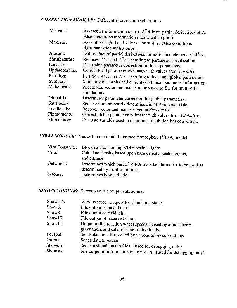
CORRECTION MODULE: Differential correction subroutines
Makeata:
Makerhs:
Atasum:
Shrinkatarhs:
Localfix:
Updateparams:
Partition:
Sumparts:
Makelocals:
Globalfix:
Savelocals:
Loadlocals:
Fixmoments:
Moreorstop:
Assembles information matrix ArA from partial derivatives of A.
Also conditions information matrix with a priori.
Assembles right-hand-side vector or Are. Also conditions
right-hand-side with a priori.
Dot product of partial derivatives for individual element of ArA.
Reduces ArA and Ar_; according to parameter specification.
Determine parameter correction for local parameters.
Correct local parameter estimates with values from Localfix.
Partition ArA and ATe according to local and global parameters.
Sum previous orbits and current orbit local parameter information.
Assembles vector and matrix to be saved to file for multi-orbit
simulations.
Determines parameter correction for global parameters.Send vector and matrix determined in Makelocals to file.
Recover vector and matrix saved in Savelocals.
Correct global parameter estimates with values from Globalfix.
Evaluate variable used to determine if solution has converged.
VIRA2 MODULE:
Vira Constants:
Vira:
Getwhich:
Setbase:
Venus International Reference Atmosphere (VIRA) model
Block data containing VIRA scale heights,
Calculate density based upon base density, scale heights,and altitude.
Determines which part of VIRA scale height matrix to be used as
determined by local solar time.
Determines base altitude.
SHOWS MODULE:
Show 1-5:
Show6:
Show8:
Show 1O:
Show 11 :
Foutput:
Output:Showerr:
Showata:
Screen and file output subroutines
Various screen outputs for simulation status.
File output of model data.
File output of residuals.
File output of observed data.
Output to file reaction wheel speeds caused by atmospheric,
gravitation, and solar torques, individually.
Sends data to a file, called by various Show subroutines.
Sends data to screen.
Sends residual data to files. (used for debugging only)
File output of information matrix ArA. (used for debugging only)
66

Show,hs:
Gameover:
Showend:
Showderivate:
Writelog.
File output of right-hand-side vector or A_8. (used for
debugging only)Indicates end of a successful run.
Send parameter solutions to "end" files
File output of partial derivative,, of ,,ensitivity matrix. (used for
debugging only)
Output to "log" file various statistic,, _i completed run.
MATRIX MODULE:
Transpose:
Multiply:
Subtract:
Add:
Inverse:
Ludcmp:Lubksb:
Matrix manipulation toolbox
Transpose a matrix.
Multiply two matrices.Subtract two matrices.
Add t_vo matrices.
Invcrta matrix.
LU Decomposition, called by lnver.rr.
LU Back substitution, called by Ludcmp.
MISC MODULE:
Ceil:
Floor:
Normal:
Cross:
Clearay:Zero:
Num2string:Standard:
Mean2:
Monther:
Clearscr:
Dayofyear:Between:
Endtoduh:
Miscellaneous mathematic and utility subroutines
Round up to nearest integer.
Round down to nearest integer.
Normalize a vector.
Evaluate cross product.
Zero various matrices.
Called by Clearav.
Convert 5 digit integer to 5 character string.
Calculate standard deviation.
Calculate mean.
Convert character representation of month to integer.
Clear screen.
Determine day of year from date.
Determine angle between two vectors.
After solution convergence, moves estimates from "end" files to
"dub" files.
67

D.2 File Interaction
Various input and output files interact with the main driver during program
execution. For these explanations, question marks (?) indicate run version number.
Version numbers are used to indicate a particular combination of parameters for
estimation. This allows the execution of more than one program version at a given time
without file usage conflict. Three x's (xxx) indicate day of year number. Five y's (yyyyy)
indicate orbit number.
orbit?.txt Orbit simulation specification.
pre?.txt: Program input: Change data window time? Y/N
if yes: Start time (minutes before periapsis)
End time (minutes after periapsis)
Time step (seconds)
(return to first question)
Change data rate? Y/N
Send observed data to screen'? Y/N
Send unfiltered observed data to file? Y/N
Number of filter passes?
post?.txt: Program input: Send filtered observed data to file?
Send model to data file?
Send residuals to data file?
Save log file?
Save parameter estimates to flies?
Y/N
Y/N
Y/N
YfN
Y/N
68

parms?.par: Parameter estimate Boolean vector. (1 estimate / 0 do not estimate)
1. Iyy2. Izz
3. Ixy4. Ixz
5. Iy z
6. cmdyaw
7. cmdroll8. rho0
9. yaw bias
10. pitch bias11. roll bias
12. CmSyaw
13. CmSpitc h14. CmSroll
15. scale height factor in
16. scale height factor out
cmdx,z?.end/duh
rho?.end/duh
cmsx,y,z?.end/duh
normx,y,z?.end/duh
moi?.end/duh
prod?.end/duh
base?.end/duh
attack?.end/duh
iter?.end/duh
fin?.end/duh
fout?.end/duh
(Two files) Yaw and Roll aerodynamic moment
coefficients and uncertainty.
Base density and uncertainty (kg /m3).
(Three files) Yaw, Pitch, and Roll solar moment
coefficients and uncertainty.
(Three files) Yaw, Pitch, and Roll norm of residuals
squared.
Mass moments of inertia and uncertainties (kg. m2).
Mass product of inertia and uncertainties (kg. m 2).
Base altitude (km).
Angles of attack: alpha and phi (rad).
Iterations for convergence.
Scale height correction factor and uncertainty (entry).
Scale height correction factor and uncertainty (exit).
69

sh?.end/duh Venusshadowentryandexit time(secondssinceperiapsis)
"end" files savevaluesaftereachiterationwhile "duh" files only containfinal estimate.Inputdatafiles are,
prtsum.xxx
rwbin.xxx
q4.obs
Orbital elements.
Binaryreactionwheelspeeds.
Quaternions.
Threefiles areusedto savereactionwheelandresiduaidata.
obsyyyyy.dat ObservedMagellanreactionwheelspeed(rad/sec).
modyyyyy.datModel reactionwheelspeed(rad/sec).
erryyyyy.dat Residual(error)of reactionwheelspeed(rad/sec).
D.3 Miscellaneous Software
The following FORTRAN (.for), Matlab (.m) and batch (.bat) files are used to
supplement MACDAS software.
angles.for:
anglesp.for
count.for
lookbin.for
Determines various geometric parameters including orbital elements,
angles of attack, Earth/Venus position, day of year, local solar time,
solar array position, sun-Venus-Earth angle, inclination of the plane
of the sky, solar longitude, and solar latitude.
Similar to angles.for except that all values are based upon future orbital
predicts.
Used to create orbit?.txt files.
Used to send binary formatted rwbin.ddd to screen.
70

makeobs.for
common.for
makesh.for
pvc.for
qcal.for
quat.for
quatsign.for
remove.for
rw2binb.for
rwmake.for
interpq.m
qp.m
cleanend.bat
Converts rwbin.ddd binary files into text files for specified time
domain.
Uses VIRA scale heights to make cmdx,y,z?.end files represent base
densities at a common base altitude. Requires base'?.end file.
Calculates scale heights required to fit given base densities.
Generates modeled solar array mass moments of inertia.
Predicts quaternions.
Extracts quaternions from quatddd.drf files.
Makes signs of quaternions appropriate for interpolation.
Removes "blunder points" from all .duh files.
Convert tach data from ASCII to binary format.
Covert tach data from tachyyddd.drf format to RW.ddd format.
Interpolate for missing quaternions.
Plots model, observed, and residuals fl)r reaction wheel data.
Deletes all "end" files.
? indicates version number
yy indicates year
ddd indicates day of year
71

D.4 Magellan Driver Routine Flow Chart
I iterate= I I
,4,set parameters for estimation I
and version number Iinteract
,V
I set first spacecraft [I] Iand a priori information
firstbaseimu
4`
determine orbits Ito be simulated
manyorbits
,d,,[ initial guess for [[ local parameters I[ firstlocs
4`___ set orbit data time windowsettime
4,read orbital elements Isetorbit I
,L
[ read reacti°nwheeldataIgetreal
4,into variable names
renameparams
4,
I determine solar ]array offpoint [
gettilt [
I determine solar [array angle [
getpvangle I
Idifferential correction
makelocals, sumparts,save locals, makeata,maker hs, s hrinkatarhs
add bias to model ]addbias
,pinterpolate model time
to real data timetimematch
Tintegrate torqueconvert, integrate [
,p
simulation [twobody, dragcalc I
solar, gravity I
Icalculatesolar_ay"lH dew,minelocal_lartimesIand add to bus [I] and appropriate scale heights I
getipvc getlst, getwhich I
output results Ishow5,6,10,11
writelog
T_ smoothdata [smoothpfs
correct global parameters
globalJix,Jixmoments
4,
[__ correct local parametersloadlocals, localcorrectio_
updateparamsI final output ]
Iendtoduh ]
evaluate iteration criterion Imoreorstop [
72

E. Cycle Four History
x 104
_i.038
O
1 . 037
i . _00 6000 6500 70'00 7500
0 L-__
ORBIT NLTM B ER
Figure E.1 Semimajor Axis
0,402[ • _ • --_ _.... • _ .
/0.4
BOO0
P4
od(D
n
H
tO
°'3%%'_o 60oo
96 .4[
96 . 3[
6500 7000 7500
ORBIT NUMBER
Figure E.2 Eccentricity
/
///
6000 6500 "2000
ORBIT A[U_BER
7500
Figure E.3 Inclination (J2000)
_3
8000
8000
73

-59.2
0
-59 . 3O
C9
mu -59.4
0
doz
-59 5,_'00 6000 6500 7000 7500
ORBIT NUMBER
8000
Figure E.4 Longitude of Ascending Node (J20O0)
ra_
r.,D
,<HI4n_
O
(_9
<
1501 .... ___ _ .....
-- 60'00 ' ----_,00 6500 7000 7500 8000
ORBIT NUMBER
Figure E.5 Argument of Periapsis (J2000)
185
180u]
o9
<
175
,<
c_
_ 171
i_ 65i00 70ioo "75'00_00
ORBIT NUMBER
/60'00
Figure E.6 Altitude at Periapsis
74

_180#3#3o_ 160t9#3A_140
cn 120
5,4o
#4 i00
80O 60
ZO_ 40
Za 20
rJ
_ s%oo
2OO
180
_ 160
140
C_
_120
#3A_i00[-4_-4
(3 80ZO_3
6O
_ 4oO
20
5%00
2O
60'00 65_00 70'00 7500
ORBIT NUMBER
Figure E.7 Inclination of Plane of Sky
8OOO
6000 6500 70J00
ORBIT NUMBER
75'00 8 00
Figure E.8 Solar Longitude
aO3
_< 15
U_ 10(_.1ZH
m 5
#3[-_
o
Z -5
O
[-,
_ -10
I:D
8 -_%'oo
SOLID: ENTRY
DASHED :
f, ',
60'00 65'00 7000 7500
ORBIT NUMBER
Figure E.9 Solar Occultation
EXIT
8O0O
75

180 _ ,
_o .......... ...._ _............
12o .... I\ ....
8o ........ ................. ......
i°° ½ I I_°o- II J " ]
01 I I i i J
5500 6000 6500 7000 7500 8000ORBIT NUMBER
Figure E.10 Solar Array Angle Theta
_360
,_340
320
[_300
o1280
260
5600 58J00 60'00 62100 64J00 6600
ORBIT NUMBER
Figure E.11 Orbit Number and Day of Year (1992)
150
,-4
I0(
U
N 5c
' T
6600 6800 7000 7200 7400 7600ORBIT NUMBER
Figure E.12 Orbit Number and Day of Year (1993)
76

_25
zc_
_2ozu]
o15
v
_I0
5o
,<
5"_'0 0 6 0'0 0 6 5'0 0
ORBIT NUMBER700O
Figure E.13 Orbit Number and Local Solar Time
_12
Z
O3
_ 6
0
_ 4rxl
_ 2
0 0CO
<
_6{'00 70'00 72'00 74'00 76'00ORBIT NUMBER
7800
Figure E.14 Orbit Number and Local Solar Time
80[DASHED LINE: SPACECRAFT ROLL (DEGREES)
60_SOLID LINE: SOLAR ARRAY OFF-POINT (DEGREES
I
aob -1
:-/- ::..............
-201
-40
DOT-DASHED LINE: SAMPLE PERIOD
(HIGH: 2/3 SECONDS LOW: 20 SECONDS)
00 6000 6500 7000 7500 8000ORBIT NUMBER
Figure E.15 Spacecraft Roll Angle, Solar Off-Point Angle, Data Rate
77

30
25
_ 2O
_ 15
_ 10
_ 5
o _:2-15
-%%oo
300
250
N_200
m 150
_100
_ 50
(,3
505'00
60'00 65'00 70'00 75'00
ORBIT NUMBER
Figure E.16 Solar Latitude
8OOO
CONJUNCTION ORBIT #7164
60'00 65'00 7000 75'00
ORBIT NUMBER8OOO
Figure E.17 Sun-Venus-Earth Angle
78

F. Reaction Wheel Data Logistics
Data required for reaction wheel analysis is stored on VAX/VMS workstation at
the Jet Propulsion Laboratory in Pasadena, California. This data includes prtsum (orbital
elements), quat (quaternions), and tach (reaction wheel speeds) files. In general, each file
represents data for one Earth day, and therefore contains information for approximately
eight Magellan orbits. Files are copied to an intermediate VAX/VMS machine at the
NASA Langley Research Center and then transferred to a personal computer. Before this
information can be processed by the MACDAS software, some pre-processing must be
performed for the tach and quat files.
Tach files are placed on a Langley VAX/VMS computer using the filename
TACHyyddd.DRF, where yy is 92, 93, or 94, and ddd represents the day of year. The
program makerw.for removes unwanted characters from the TACHyyddd.DRF file and
places results in the file RW.ddd. This ASCII file contains time and three reaction wheel
speeds. A second program called rw2binb.for converts the ASCII file into binary as the
file RWBIN.ddd. The binary formatted file is the observed reaction wheel speed input
file for MACDAS. Both RW.ddd and RWBIN.ddd are backup up using a tape drive
system. Cycle Five data has the designation RW5.ddd and RWBIN5.ddd for reaction
wheel files.
Quat files also required pre-processing belore use with MACDAS. Since
quaternions (spacecraft attitude) change very little for each orbit, it is only necessary to
know and store the quaternions for the instant of periapsis rather than the entire orbit.
The program quat.for is used to search QUATddd.DRF for the quaternions that represent
spacecraft attitude near periapsis. Again, ddd represents day of year. In order to find the
correct quaternions within a particular QUATddd.DRF file, the time of periapsis must be
know. This information is retrieved by the quat program from the appropriate
PRTSUM.ddd file. Output from the quat.for program is a file containing orbit numbers
79

and corresponding quaternions. For a few orbits, quaternions are not found within
QUATddd.DRF files. These missing values may be determined from an interpolation
between known quaternions since the changes in spacecraft attitude (at periapsis) are
gradual. The Matlab program interpq.m is used to perform this interpolation. Care must
be take to correctly interpolate these quaternions since an attitude does not uniquely
determine a set of quaternions. That is, a sign change of all quaternions does not alter
spacecraft attitude. The program quatsign.for may be used to insure that signs are such
that the interpolation will be done correctly. The final data file for quaternions is
Q?.OBS, where ? is either 4 for Cycle Four, or 5 for Cycle Five. This file contains orbit
numbers and quaternions for each orbit near periapsis which is used by MACDAS.
PRTSUM.ddd files require no special pre-processing before use with MACDAS.
80

References
1. D. King-ltele, Satellite Orbits in an Atmosphere: Theory and Applications,
Blackie, 1987.
2. tl. Curtis, "Magellan: Aerobral:ing at Venus," Aerospace Anterica, vol. 32, no. 1,
pp. 32-36, January 1994.
3. D. Lyons, "Aerobraking Magellan: Plan versus Reality," AAS-94-118, American
Astronautical Society / American lnslitute of Aeronautics and A_tronautics Space
Flight Mechanics Meeting, Cocoa Beach, Florida, February 1994.
4. P. Marsden and C. Croom, "Determining Atmospheric Density and Spacecraft
Aerodynamic Properties from Magellan Attitude Data," American Institute of
Aeronautics and Aslronautics Mid-Atlantic Regional Student Conference,
Annapolis, Maryland, April 1993.
5. P. Marsden, "Determining the Atmospheric Density of Venus and Magellan
Aerodynamic Properties from Spacecraft Attitude Data," M. S. Thesis, The
George Washington University, June 1993.
6. C. Croom and R. Tolson, "Using Magellan Attitude Data to Study Venusian
Atmosphere and Various Spacecraft Properties," AAS-94-141, American
Aslronautical Society / American Institute of Aeronautics and Astronautics Space
Flight Mechanics Meeting, Cocoa Beach, Florida, February 1994.
7. G. M. Kealing, A. J. Kliore, and V. 1. Moroz, "Venus International Reference
Atmosphere," Advances in Space Research, vol. 5, No. 1 I, 1985.
8. D. T. Lyons, "Magellan: Planetary Constants and Models," JPL D-2300, Rev. E,
April !, 1992, sect. 2-1.
9. D.T. Lyons, "Magellan: Planetary Constants and Models," JPL D-2300, Rev. E,
April 1, 1992, sect. 2-22.
I0. National Aeronautics and Space Administration, Magellan: The Unveiling of Vemts.
JPL 400-345 3/89, March 1993, pp. 23.
I I. D. Doody, "Magellan Mapping Update: A Matter of Gravity," Aerospace America,
vol. 31, no. 5, May 1993, pp. 20-24.
12. R. Fredo and M. Kaplan, "Procedure fi_r Obtaining Aerodynamic Properties of
Spacecraft," AIAA-81-4214, Journal ¢_Spacecrqft, vol. 18, no. 4,
July-August, 198 I.
81

13. L. Meirovitch,Methods of Analytical Dynamics, McGraw-Hill, New York, 1971,
pp.437.
14. D. Marguardt, "An Algorithm for Least Squares Estimation of Nonlinear
Parameters," Journal of SIAM, vol. 2, 1963, pp. 431-441.
15. R. E. Maine, K. W. Iliff, "Identification of Dynamic Systems," AGARD-AG-3000,
1984, ch. 11.
16. G. M. Keating, N. C. Hsu, "The Venus Atmospheric Response to Solar Cycle
Variations," Geophysical Research Letters, vol. 20, No. 23, December 1993,
pp. 2752-2754.
17. D. T. Lyons, "Magellan: Planetary Constants and Models," JPL D-2300, Rev. E,
April I, 1992, sect. 8-3.
82
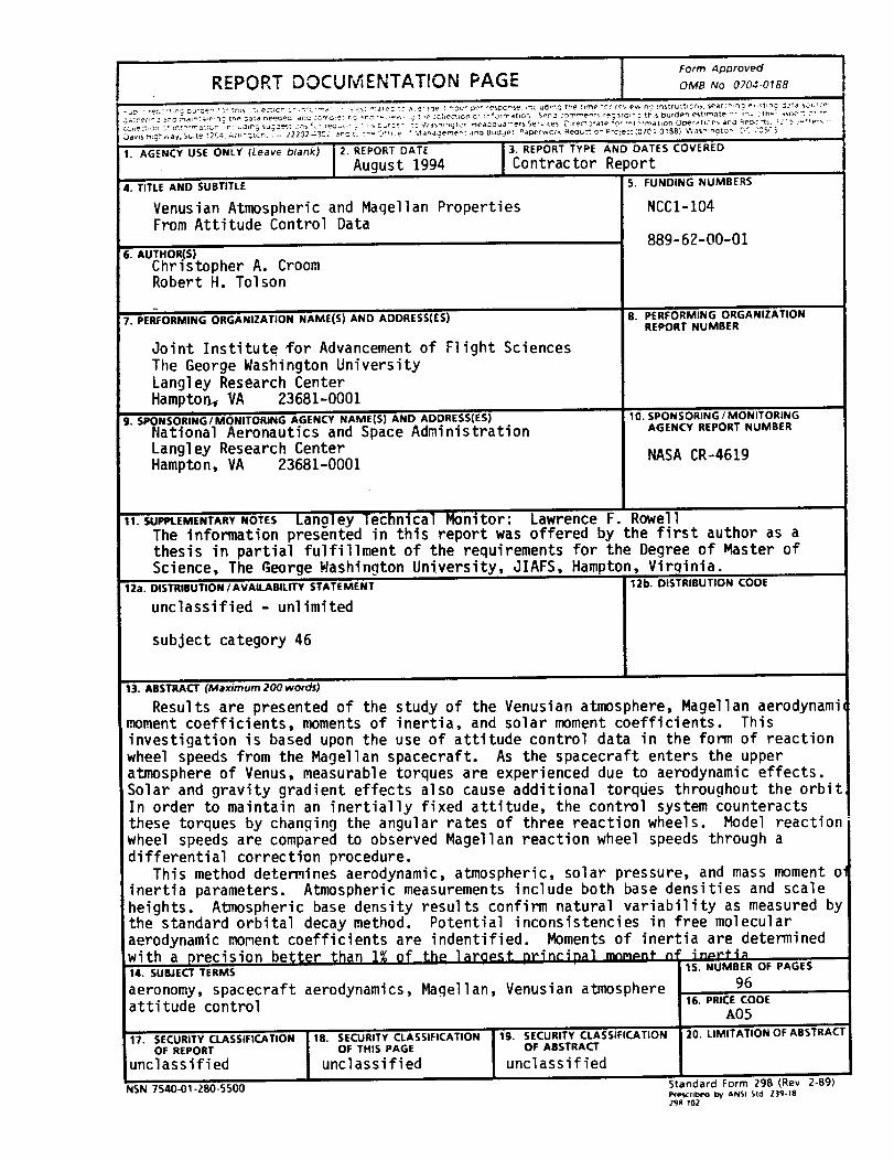
I Form AporovedREPORT DOCUMENTATION PAGE OM_Ivo o_o.:-o,88
_,Liie-'_,OnL_ _n,?-_r_:;_r, .__'I_P_ _u_._ Cn_ f_r r_oF _ _,_:s_r-_ _ _C ¢_h_n<_o_ _ea_ar_ers Se'_,ce_ _;rec_,a_e _c,"'_t_rr_atlon OOt_r_tlcr_ an_ _e_r_s _!_ elders.'"
_av_ H::_-;.a_. _,_,_te 204 ,k:_l_',cr,, .:, 2220_3S_ _r_. t: "_o _'_ :_, _" ',_a_a_emer,_ a_o 8u_ge'. PaDe. rwot_ Re_nu_ O_ Pre_e=: _CTQ4-01B8)_a_m_ng_on I'_C2C5C _.
' l4. TITLE AND SUBTITLE 5. FUNDING NUMBERS
Venusian Atmospheric and Magellan PropertiesFrom Attitude Control Data
6. AUTHOR(S)
Christopher A. CroomRobert H. Tolson
7. PERFORMING ORGANIZATION NAME(S) AND ADDRESS{ES)
Joint Institute for Advancement of Flight Sciences
The George Washington UniversityLangley Research CenterHampto_ VA 23681-0001
g. SPONSORING/MONITORINGAGENCYNAME(S)AND ADDRESS(ES)National Aeronautics and Space AdministrationLangley Research CenterHampton, VA 23681-0001
NCC1-I04
889-62-00-01
B. PERFORMING ORGANIZATIONREPORT NUMBER
10. SPONSORING / MONITORINGAGENCY REPORT NUMBER
NASA CR-4619
11.SUPI_LEMENTARYNOTES Lanoley Technical Monitor: Lawrence F. RowellThe information presented in this report was offered by the first author as a
thesis in partial fulfillment of the requirements for the Degree of Master of
Science, The George Washington University, JIAFS, Hampton, Virginia.12a. OISTRIBUTION/AVAILABILITY STATEMENT 12b. DISTRIBUTION CODE
unclassified - unlimited
subject category 46
13. ABSTRACT (Maximum 200wor_)
Results are presented of the study of the Venusian atmosphere, Magellan aerodynamimoment coefficients, moments of inertia, and solar moment coefficients. Thisinvestigation is based upon the use of attitude control data in the form of reaction
wheel speeds from the Magellan spacecraft. As the spacecraft enters the upperatmosphere of Venus, measurable torques are experienced due to aerodynamic effects.
Solar and gravity gradient effects also cause additional torques throughout the orbitIn order to maintain an inertially fixed attitude, the control system counteractsthese torques by changing the angular rates of three reaction wheels. Model reaction
wheel speeds are compared to observed Magellan reaction wheel speeds through adifferential correction procedure.
This method determines aerodynamic, atmospheric, solar pressure, and mass moment o"inertia parameters. Atmospheric measurements include both base densities and scale
heights. Atmospheric base density results confirm natural variability as measured bythe standard orbital decay method. Potential inconsistencies in free molecular
aerodynamic moment coefficients are indentified. Moments of inertia are determinedwith a recision better " •14. SU_ECT TERMS
aeronomy, spacecraft aerodynamics, Magellan, Venusian atnmsphereattitude control
17. SECURITY CLASSIFICATIONOF REPORT
unclassified
NSN 7540-01-280-5500
18. SECURITY CLASSIFICATION ]
OF THIS PAGE
unclassified
19. SECURITY CLASSIFICATIONOF ABSTRACT
unclassified
1S. NUMBER OF PAGES
9616. PRICE CODE
A0520. LIMITATION OF ABSTRACT
Standard Form 298 (Rev 2-89)Prc,_r=tx.d by ANSI _td Z39-1829R-102


![[PPT]Ferdinand Magellan - Tripod.comwadd.tripod.com/Magellan.ppt · Web viewFerdinand Magellan By Taylor and Haley Magellan was born in spring in 1470. Magellan was killed in the](https://cdn.vdocuments.net/doc/165x107/5afc89fd7f8b9a814d8c3915/pptferdinand-magellan-viewferdinand-magellan-by-taylor-and-haley-magellan-was.jpg)


