Download - Voter interacting systems applied to Chinese stock markets

Journal Identification = MATCOM Article Identification = 3656 Date: June 16, 2011 Time: 11:26 am

Available online at www.sciencedirect.com

Mathematics and Computers in Simulation 81 (2011) 2492–2506

Original article

Voter interacting systems applied to Chinese stock markets

Tiansong Wang, Jun Wang ∗, Junhuan Zhang, Wen FangDepartment of Mathematics, College of Science, Beijing Jiaotong University, Beijing 100044, PR China

Received 23 November 2008; received in revised form 14 March 2011; accepted 30 March 2011Available online 17 April 2011

Abstract

Applying the theory of statistical physics systems – the voter model, a random stock price model is modeled and studied inthis paper, where the voter model is a continuous time Markov process. In this price model, for the different parameters values ofthe intensity λ, the lattice dimension d, the initial density θ, and the multivariate set (θ, λ), we discuss and analyze the statisticalbehaviors of the price model. Moreover, we investigate the power-law distributions, the long-term memory of returns and thevolatility clustering phenomena for the Chinese stock indices. The database is from the indices of Shanghai and Shenzhen in the6-year period from July 2002 to June 2008. Further, the comparisons of the empirical research and the simulation data are given.© 2011 IMACS. Published by Elsevier B.V. All rights reserved.

Keywords: Stock price model; Voter model; Probability distribution; Return; Computer simulation

1. Introduction

As the governments deregulate the stock markets, it is becoming an important problem to model the dynamics ofthe forwards prices in the risk management, derivatives pricing and physical assets valuation. And the research workon the statistical properties of fluctuations of stock prices in globalized securities markets is also significant. Recently,some research work has been done, by applying the interacting particle systems, to investigate the statistical behaviorsof fluctuations of stock prices, and to study the corresponding valuation and hedging of contingent claims, for instancesee [11,12,17,21,22]. Stauffer and Penna [21] and Tanaka [22] have been apply the percolation model to study themarket fluctuation, see [8]. In [21,22], they construct the local interaction or influence among investors in a stockmarket and define the cluster of investors with the same opinion about the market as a cluster of percolation. In theirfinancial models, they suppose that the stock price fluctuation is influenced by the information in the stock market, andthe investors follow the effect of sheep flock. That means that the investors decide the investment opinions by otherinvestors’ attitudes, so the investors’ investment attitudes of the stock market lead to the stock price fluctuation. In thepresent paper, we apply a statistical physics model – the voter model (see [3,15]) to study the fluctuation behaviors ofthe return processes. Through the computer simulation on this financial model, we discuss the statistical behavior, thetail behavior, long term memory of fluctuation and the volatility clustering phenomena for the return processes.

In recent years, the empirical research in financial market fluctuations has been made. Some statistical properties formarket fluctuations uncovered by the high frequency financial time series, such as fat tails distribution of price changes,the power-law of logarithmic returns and volume, volatility clustering which is described as on-off intermittency in

∗ Corresponding author. Fax: +86 10 51682867.E-mail address: [email protected] (J. Wang).

0378-4754/$36.00 © 2011 IMACS. Published by Elsevier B.V. All rights reserved.doi:10.1016/j.matcom.2011.03.013

dx.doi.org/10.1016/j.matcom.2011.03.013

mailto:[email protected]

dx.doi.org/10.1016/j.matcom.2011.03.013


T. Wang et al. / Mathematics and Computers in Simulation 81 (2011) 2492–2506 2493

Fig. 1. The chart of the voter model.

literature of nonlinear dynamics, and multifractality of volatility, etc., see [1,5–7,9,10,12,14,16–19]. China has twostock markets, Shanghai Stock Exchange and Shenzhen Stock Exchange, and the indices studied in this paper areShanghai Stock Exchange Composite Index (SSECI) and Shenzhen Stock Exchange Component Index (SZSECI).These two indices play an important role in Chinese stock markets and Chinese economic systems. In this paper, weanalyze the daily data of SSECI and SZSECI from July 1st 2002 to June 30th 2008, and study the fluctuation propertiesof SSECI and SZSECI. The database of the indices is from the websites www.sse.com.cn and www.szse.cn.

First, we give the brief definitions and properties of the voter model, and also we introduce the graphical representa-tion of the model, since the graphical representation is necessary for our computer simulations. One interpretation forthe voter model is, for a collection of individuals, each of which has one of two possible positions on a political issue,at independent exponential times, an individual reassesses his view by choosing a neighbor at random with certainprobabilities and then adopting his position. Specifically, the voter model is one of the statistical physics models, wethink of the sites of the d-dimensional integer lattice as being occupied by persons who either in favor of or opposedto some issue. To write this as a set-valued process, we let ηs is the set of voters in favor, we can also think of the sitesin ηs as being occupied by cancer cells, and the other sites as being occupied by healthy cells. We can formulate thedynamics as follows: (i) an occupied site becomes vacant at a rate equal to the number of the vacant neighbors; (ii) anvacant site becomes occupied at a rate equal to λ times the number of the occupied neighbors, where λ is a intensitywhich is called the “carcinogenic advantage” in voter model. When λ = 1, the model is called the voter model, andwhen λ > 1, the model is called the biased voter model.

For simplicity, we give the construction of graphical representation for 1-dimensional voter model (λ = 1), for moregeneral cases, see [3,15]. Thinking of 1-dimensional integer points as being laid out on a horizontal axis, with the timelines being placed vertically, above that axis. Define independent Poisson processes with rate 1 for each time lines, ateach event time (u, s), we choose one of its two neighbors with probability 1/2, and draw an arrow from that neighborpoint to (u, s), and write a δ at (u, s), see Fig. 1. To construct the process from this “graphical representation”, weimagine fluid entering the bottom at the points in η0 and flowing up the structure. The δ′s are the dams and the arrowsare pipes which allow the fluid to flow in the indicated direction. For example in above Fig. 1, fluid can flow from thesite (− 2, 0) to the site (0, t). Let ηA

s denote the state at time s with the initial state ηA0 = A, then from [1,14], the voter

model ηAs approaches total consensus in d = 1 and d = 2. But in higher dimensions d ≥ 3, the differences of opinion may

persist. For more generally, we consider the initial distribution as νθ , the product measure with density θ, that is, eachsite is independently occupied with probability θ and let ηθ

s to denote the voter model with initial distribution νθ . Let

η{0}s = {0}, and η

{0}s (u) be the state of u ∈ Z

d at time s with the initial point {0}.

More formally, the stochastic dynamics of the voter model ηs is a Markov process on Ω = {0, 1}Zdwhose generator

has the form

Af (η) =∑

u

c(u, η)[f (ηu) − f (η)]

http://www.sse.com.cn

http://www.szse.cn


2494 T. Wang et al. / Mathematics and Computers in Simulation 81 (2011) 2492–2506

where the functions f (on Ω) depend on finitely many coordinates, and ηu(v) = η(v) if v /= u, ηu(v) = −η(v) if v = u,for u, v ∈ Z

d . c(u, η) is the transition rate function for the process which is given by follows (see [1,14]), for anyη ∈ Ω = {0, 1}Zd

c(u, η) =

⎧⎪⎪⎨⎪⎪⎩

∑v

p(u, v)η(v) if η(u) = 0

∑v

p(u, v)[1 − η(v)] if η(u) = 1

where p(u, v) ≥ 0 for u, v ∈ Zd , and

∑vp(u, v) = 1 for all u ∈ Z

d . And we assume that p(u, v) is such that the Markovchain with those transition probabilities is irreducible.

For the biased voter model (λ > 1), there is a “critical value” for the process, that is, on Ω = {0, 1}Zdand with the

corresponding probability P, the critical value λc is defined as

λc = inf{λ : P(|{0}ηs| > 0, for all s ≥ 0) > 0}

where |η{0}s | is the cardinality of η

{0}s . Suppose λ > λc, then there is a convex set C so that on Ω∞ = {η{0}

s /= ∅, for all s},we have for any ε > 0 and for all s sufficiently large (see [3,15])

(1 − ε)sC ∩ Zd ⊂ η{0}

s ⊂ (1 + ε)sC ∩ Zd

If λ < λc, for some positive ρ(λ), we have

P(η{0}s /= ∅) ≤ e−ρs

The above results imply that, on d-dimensional lattice, if λ < λc, the process dies out (becomes vacant) exponentiallyfast, if λ > λc, the process survives with the positive probability.

2. Modeling a stock price model by the voter dynamic systems

In this part, the return process of a stock price on d-dimensional integer lattice is constructed, based on the votermodel. We assume that the information in the stock market lead to the fluctuation of a stock price, and there are threekinds of information: buying information, selling information and neutral information. And the fluctuation of a stockprice relies on the investor’s investment attitudes, which accordingly classify buying stock, selling stock and holdingstock. Consider a model of auctions for the same stock defined above, we can derive the stock price process fromthe auctions. Assume that each trader can trade the stock several times at each day t ∈ {1, 2, . . ., n}, but at most oneunit number of the stock at each time. Let l be the time length of trading time in each trading day, we denote thestock price at time s in the t th trading day by St(s), where s ∈ [0, l]. Suppose that this stock consists of m2 + 1 (m2 islarge enough) investors, who are located in a line {−m2/2, . . . , −1, 0, 1, . . . , m2/2} ⊂ Z (similarly for d-dimensionallattice Z

d). At the beginning of trading in each day, suppose that only the investor at the site {0} receives some news.We define a random variable ξt({0}) for this investor, suppose that this investor taking buying position (ξt({0}) = 1),selling position (ξt({0}) = − 1) or neutral position (ξt({0}) = 0) with probability p1, p−1 or 1 − (p1 + p−1) respectively.Then this investor sends bullish, bearish or neutral signal to his nearest neighbors. According to d-dimensional voterprocess system, investors can affect each other or the news can be spread, which is assumed as the main factor of pricefluctuations for the investors. Moreover, here the investors can change their buying positions or selling positions toneutral positions independently at a constant rate. More specifically, (I) when ξt({0}) = 1 and if η

{0}s (u) = 1, we say

that the investor at u takes buying position at time s, and this investor recovers to neutral position 0 at a rate equalto the number of the vacant neighbors; if η

{0}s (u) = 0, we think the investor at u takes neutral position at time s, and

this investor is changed to take buying position by his nearest neighbors at rate λ∑

v:|v−u|=1η{0}s (v). In this case, the

more investors with taking buying positions, the more possible the stock price goes up. (II) When ξt({0}) = − 1 and ifη

{0}s (u) = 1, we say that the investor at u takes selling position at time s, also this investor recovers to neutral position 0

at a rate equal to the number of the vacant neighbors; if η{0}s (u) = 0, the investor is changed to take selling position by



0 100 200 300 400 500 600 700 800 900 10009.4

9.6

9.8

10

10.2

10.4

10.6

10.8

11

11.2

11.4

Days

Pric

es

Fig. 2. The fluctuations of the stock prices model.

his nearest neighbors at rate λ∑

v:|v−u|=1η{0}s (v). (III) When the initial random variable ξt({0}) = 0, the process η

{0}s (u)

is ignored, this means that the investors do not affect the fluctuation of the stock price.For a fixed s ∈ [0, l] (l large enough), let

Bt(s) = ξt({0}) |η{0}s |

m2(n), s ∈ [0, l]

where |η{0}s | = ∑m2/2

u=−m2/2η{0}s (u), and m2 depends on the trading days n. From above definitions and [1,12,19,22], we

define the stock price at t th trading day t(t = 1, 2, . . ., n) as

St(s) = eαBt (s)St−1(s), s ∈ [0, l]

where α > 0, represents the depth parameter of the market. Then we have

St(s) = S0 exp{αt∑

k=1

Bk(s)}, s ∈ [0, l]

where S0 is the stock price at time 0. According to the theory of the voter process (see [15]) and above definitions, ifλ > λc, the news will spread widely, so this will affect the investors’ positions, and finally will affect the fluctuation ofthe stock price. If λ ≤ λc, the influence on the stock price by the investors is limited.

Next we define the returns of stock prices, see [13,20,23], we have the formula of the stock logarithmic return asfollows

r(t) = lnSt+1(s)

St(s), t = 1, 2, . . . , n

In this paper, we analyze the logarithmic returns for the daily price changes. In the followings, we let s = 2000,then we plot the fluctuations of the stock prices and the corresponding returns by simulating the one-dimension votermodel, see Figs. 2 and 3.

3. Data analysis by the computer simulation

In recent years, the probability distribution in the financial market fluctuation has been studied, the empiricalresearch results show that the distribution of the large returns follow a power-law distribution with the exponent 3, thatis P(r(t) > x) ∼ x−μr , where r(t) is the returns of the stock prices in a given time interval �t, μr ≈ 3, for example see[5,9,10,14,19]. In this section, Section 3.1 presents the statistical analysis of the simulation data for univariate process.



0 100 200 300 400 500 600 700 800 900 1000−0.03

−0.02

−0.01

0

0.01

0.02

0.03

Days

Ret

urns

Fig. 3. The fluctuations of market returns.

Section 3.2 investigates the returns for multivariate process. Finally, in Section 3.3, the conclusions of the analysisbetween univariate process and multivariate process are summarized.

3.1. Analysis for univariate process

In this section, we discuss the three parameters of the financial model, the intensity λ, the lattice dimension d, theinitial density θ (or the initial distribution νθ of the model). And we show some figures and tables to describe thepower-law distribution of the returns for the simulation data. Further, we compare the power-law distribution of thereturns with the corresponding Gaussian distribution, and study the statistical properties of the price model by thedifferent values of one parameter. First, we discuss the behaviors of the returns for the different values of λ.

According to the computer computations in Table 1, the kurtosis is increasing steadily with the parameter λ increas-ing, while the exponent μ is decreasing with the value λ increasing, for the fixed values d = 1, θ = 0.1. When λ = 5,the kurtosis value is the smallest while the value μ is the biggest in the five groups simulation data, 3.248 and 5.444respectively; when λ = 25, the situation is reverse. Moreover, we can see that the fat tail behavior of the returns ismore significantly as λ increases in Fig. 4. These results imply that the parameter λ, which represents the rate ofinformation spread in the price model, can affect the power-law distributions of the price returns. Fig. 4 also showsthat the probability distributions of the returns deviate from the corresponding Gaussian distribution.

In Fig. 5 and Table 2, we continue to study the statistical properties of the price returns with the different latticedimensions d for the fixed values λ = 5, θ = 0.1. In Fig. 5, the tails of the distributions are deviating from that of thecorresponding Gaussian distribution as the dimension d increases, this implies the fat-tails phenomena is much obviousin this case. Similarly to the results of Tables 1 and 2 also show that the kurtosis of the model is increasing and theexponent μ is decreasing for the parameter d. When d = 3, the value of kurtosis is 8.033, which is the biggest, and μ

is 3.658, the smallest value in three groups data. The reason of these increasing (or decreasing) properties is that the

Table 1The statistical analysis of the returns for the intensity λ.

λ Min Max Mean Variance Kurtosis Skewness μ

5 −0.0317 0.0227 −6.135 × 10−5 5.711 × 10−5 3.248 −0.0156 5.44410 −0.0368 0.0396 2.989 × 10−4 1.641 × 10−4 3.701 −0.0231 5.18115 −0.0345 0.0296 1.707 × 10−4 4.194 × 10−5 4.163 0.0129 4.21320 −0.0413 0.0404 −4.562 × 10−4 4.558 × 10−4 4.304 −0.0159 3.66125 −0.0491 0.0518 −3.996 × 10−4 5.886 × 10−4 5.076 0.0182 3.477



0.01 0.02 0.03 0.04

10 −2

10 −1

10 0

|r(t)|

log(

P(|

r(t)

|>x)

)

λ=5λ=10λ=20Gaussian

Fig. 4. The cumulative distributions of the normalized price returns with the different values of λ when d = 1, θ = 0.1.

0.01 0.02 0.03 0.04

10−2

10−1

100

|r(t)|

log(

P(|

r(t)

|>x)

)

d=1d=2d=3Gaussian

Fig. 5. The cumulative distributions of the normalized price returns with the different values of d when λ = 5, θ = 0.1.

interaction among the investors becomes more active in this financial model (which is defined by the voter dynamicsystem) as the dimension d increases.

Finally, we discuss the effects of the parameter θ on the returns. θ is the initial density of the price model, and itrepresents the proportion of the investors obtaining the information at the beginning of each trading day. When the

Table 2The statistical analysis of the returns for the lattice dimension d.

d Min Max Mean Variance Kurtosis Skewness μ

1 −0.0317 0.0227 −6.135 × 10−5 5.711 × 10−5 3.248 −0.0156 5.4442 −0.0332 0.0314 4.870 × 10−5 9.220 × 10−5 5.963 −0.0123 4.7943 −0.0558 0.0517 3.074 × 10−4 5.282 × 10−4 8.033 −0.0222 3.658



0.01 0.02 0.03 0.04

10−2

10−1

100

|r(t)|

log(

P(|

r(t)

|>x)

)

θ=0.05θ=0.1θ=0.15Gaussian

Fig. 6. The cumulative distributions of the normalized price returns with the different values of θ when d = 1, λ = 20.

initial density value θ increases, the more investors will share the same opinion about the market, then the stock priceshould fluctuate more greatly. This property can been seen in Fig. 6 and Table 3.

In fact, the simulation results of the returns for the initial density θ can be extended in this financial model. Forexample, we can suppose that the initial state of the model is some random variable ξνθ (or ξνθ

t ) following a certaindistribution νθ . In a stock market, the investors usually decide their investment positions by analyzing the historicaldata on the stock, the nearer the time of the historical data is to the present, the stronger impact the data have on theinitial distribution νθ . In this case, we can introduce the Brownian motion in order to make the initial distribution havethe effect of random movement while maintaining the original trend, for the related work see [13]. It is also interestingto do the computer simulations of the returns for the different random initial distributions νθ , it can improve our modelbecause the fluctuations in the stock markets are random.

3.2. Analysis for multivariate process

In the above section, we have discussed the returns for univariate process. In this part, we study the returns formultivariate process. We analyze the statistical behaviors of the returns for the multivariate set (θ, λ). For the simplicity,let d = 1, and suppose that θ and λ satisfy a linear function aθ + bλ + c = 0, where a, b, c are three constants. In Table 4,we consider the multivariate set

{(θ, λ) : aθ + bλ + c = 0, a = 100, b = −1, c = 5}.By the computer computation, we have Table 4.From Table 4, we have the similar statistical properties as that in Section 3.1, when θ and λ increase simultaneously,

the kurtosis value increases while the value of μ decreases accordingly. However, the rise and the fall of the valuesare more dramatic. The kurtosis in the multivariate processing on (θ, λ) increases more quickly than that in the single

Table 3The statistical analysis of the returns for the initial density θ.

θ Min Max Mean Variance Kurtosis Skewness μ

0.01 −0.0320 0.0294 7.008 × 10−5 6.206 × 10−5 3.312 −0.0224 7.0320.05 −0.0345 0.0296 9.506 × 10−5 4.259 × 10−5 3.493 −0.0181 5.0790.10 −0.0413 0.0404 −4.562 × 10−4 4.558 × 10−4 4.304 −0.0159 3.6610.15 −0.0398 0.0466 5.101 × 10−4 8.574 × 10−5 4.836 −0.0274 3.4970.20 −0.0511 0.0502 4.085 × 10−5 9.612 × 10−5 7.974 −0.0209 3.125



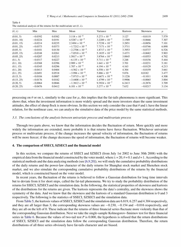
Table 4The statistical analysis of the returns for the multivariate set (θ, λ).

(θ, λ) Min Max Mean Variance Kurtosis Skewness μ

(0.01, 5) −0.0392 0.0382 3.118 × 10−4 5.273 × 10−5 3.127 −0.0119 7.579(0.01, 10) −0.0224 0.0191 4.5287 × 10−5 3.2289 × 10−5 3.1589 −0.0666 7.307(0.01, 15) −0.0214 0.0235 2.3494 × 10−4 3.7238 × 10−5 3.2851 −0.0856 7.101(0.01, 25) −0.0373 0.0373 −1.7212 × 10−4 7.7171 × 10−5 3.3711 −0.0746 6.890(0.05, 5) −0.0181 0.0130 −2.2706 × 10−4 1.8717 × 10−5 3.3953 −0.0737 6.526(0.05, 15) −0.0248 0.0261 −7.0518 × 10−5 5.1835 × 10−5 3.4371 −0.0682 5.903(0.05, 25) −0.0287 0.0213 1.5817 × 10−4 3.8764 × 10−5 3.8845 −0.0553 4.702(0.1, 5) −0.0317 0.0227 −6.135 × 10−5 5.711 × 10−5 3.248 −0.0156 5.444(0.1, 10) −0.0368 0.0396 2.989 × 10−4 1.641 × 10−4 3.701 −0.0231 5.181(0.1, 15) −0.0345 0.0296 1.707 × 10−4 4.194 × 10−5 4.163 −0.0129 4.213(0.1, 20) −0.0413 0.0404 −4.562 × 10−4 4.558 × 10−4 4.304 −0.0159 3.661(0.1, 25) −0.0491 0.0518 −3.996 × 10−4 5.886 × 10−4 5.076 0.0182 3.477(0.15, 5) −0.0104 0.0087 −7.9715 × 10−5 4.6671 × 10−6 5.1226 −0.1011 4.308(0.15, 25) −0.0176 0.0182 −3.4408 × 10−5 1.4799 × 10−5 5.9906 −0.0065 3.004(0.20, 5) −0.0064 0.0046 −1.3812 × 10−5 9.3924 × 10−7 6.2413 −0.2876 3.709(0.20, 25) −0.0476 0.0412 6.101 × 10−4 3.277 × 10−4 7.632 −0.0217 3.134

processing on θ or on λ, similarly to the case for μ, this implies that the fat-tails phenomena is more significant. Thisshows that, when the investment information is more widely spread and the more investors share the same investmentattitudes, the effect of sheep flock is more obvious. In this section we only consider the case that θ and λ have the linearrelation, for the nonlinear case, we can analyze the simulative data of the price model by the same statistical methods.

3.3. The conclusions of the analysis between univariate process and multivariate process

Through two parts above, we know that the information decides the fluctuation of return. More quickly and morewidely the information are extended, more probable it is that returns have fierce fluctuation. Whichever univariateprocess or multivariate process, if the change increases the spread velocity of information, the fluctuation of returnswill be more fiercer; if the change decreases the speed of information, the fluctuation of returns will become weaker.

4. The comparison of SSECI, SZSECI and the financial model

In this section, we compare the returns of SSECI and SZSECI (from July 1st 2002 to June 30th 2008) with theempirical data from the financial model constructed by the voter model, where λ = 20, θ = 0.1 and d = 1. According to thestatistical methods and the data analyzing methods (see [6,9,20]), we will study the cumulative probability distributionsof the daily returns and the power-law character of the daily returns for Shanghai stock market and Shenzhen stockmarket, and we also simulate the corresponding cumulative probability distributions of the returns by the financialmodel, which is constructed based on the voter model.

In recent years, the fluctuation of the returns is believed to follow a Gaussian distribution for long time intervalsbut to deviate from it for short steps, called the fat-tail phenomena. We try to study the probability distribution of thereturns for SSECI, SZSECI and the simulation data. In the following, the statistical properties of skewness and kurtosisof the distributions for the returns are given. The kurtosis represents the data’s centrality, and the skewness shows thesymmetry of the data. And we know that the skewness and the kurtosis of a standard Gaussian distribution is 0 and 3respectively. The following is the statistics of SSECI, SZSECI and the simulation data.

From Table 5, the kurtosis values of SSECI, SZSECI and the simulation data are 6.819, 6.257 and 4.304 respectively,and they are all larger than 3; the corresponding skewness values are −0.230, −0.154 and −0.016 respectively, andthey are all on the left of 0. These indicate that the returns of three financial series fluctuate more violently than that ofthe corresponding Gaussian distribution. Next we take the single-sample Kolmogorov–Smirnov test for three financialseries in Table 6. Because the values of two-tail test P is 0.000, the hypothesis is refused that the return distributionsof SSECI, SZSECI and the simulation data follow the corresponding Gaussian distribution. Therefore, the returndistributions of all three series obviously have fat-tails character and are biased.



Table 5The statistical analysis of the returns for SSECI, SZSECI and the simulation data.

Sample size Mean Variance Skewness Kurtosis μ

SSECI 1455 4.599 × 10−4 2.756 × 10−4 −0.230 6.819 2.865SZSECI 1454 8.399 × 10−4 3.309 × 10−4 −0.154 6.257 2.734Simulation 5000 −4.562 × 10−4 4.558 × 10−4 −0.016 4.304 3.661

4.1. The estimates of the long term memory for the returns

The evaluation of the long memory of one time series can be made through various methodologies. In this section,the long memory is measured by the Hurst exponent H, calculated through the classic Rescaled Range (R /S) Analysisand modified Rescaled Range (R /S) statistic.

4.2. Rescaled Range Analysis

Rescaled Range (R /S) Analysis is a very effective nonparametric test to analyze the durative of time sequences anddo not need special distributions of time sequences studied. R /S is a new statistics which can be used to distinguishwhether time sequence relies on the time, that is, the exponent of Hurst. Green and Fielitz firstly applied R /S tostudy the mathematical finance and analysis the common stock returns. The research shows that, when H = 0.5, thetime sequence belongs to Brownian motion and the variables are independent and the correlation coefficients are 0;when 0 < H < 0.5, the variables are negative correlation and are anti-persistence; when 0.5 < H < 1, that means the timesequence is persistent and has the quantification of long-term memory. In order to calculate the Hurst exponent H, thetime series xt with N numbers is divided by A parts. And each part marks as xa,k, a = 1, 2, . . ., A. For t = 1, 2, . . ., N, let

xa = 1

n

n∑k=1

xa,k, Xa,t =t∑

k=1

(xa,k − xa)

Ra = max1≤t≤NXa,t − min1≤t≤N

Xa,t, Sa =[

1

N

N∑k=1

(xa,k − xa)2

]1/2

By computing Ra/Sa by each part data, then we have the mean as follows

(R/S)N = 1

A

A∑a=1

(Ra/Sa)

The Hurst exponent H is obtained by the expression ln (R/S)N = ln C + Hln N, which is given by Mandelbrot andWallis [18], and the values of H can be calculated by the lease ordinary squares. By applying the method of the R/S test, the exponent H of the returns for SSECI, SZSECI are 0.6363, 0.6367 respectively, and the exponent H of thereturns for the price model is 0.5979, see Fig. 7. The H of three groups’ data are all larger than 0.5, which indicate thatthese three financial time sequences are all long-term memory sequences.

Table 6The Kolmogorov–Smirnov test.

Sample size H CV Two-tail test P Statistics of K–S

SSECI 1455 1 0.029 0.000 0.475SZSECI 1454 1 0.028 0.000 0.472Simulation 5000 1 0.025 0.000 0.406

Journal Identification

= M

AT

CO

M

Article

Identification =

3656

Date:

June 16,

2011

Tim

e: 11:26

am

T. W

ang et

al. /

Mathem

atics and

Com

puters in

Simulation

81 (2011)

2492–2506

2501

2 3 4 5 6 7 81

1.5

2

2.5

3

3.5

4

log(n)

log(

R/S

)

0 200 400 600 800 1000 1200 1400 1600 1800 20000.5

0.51

0.52

0.53

0.54

0.55

0.56

0.57

0.58

0.59

0.6

n

a b

The

val

ue o

f HFig. 7. The Hurst exponent of the returns for the simulation data.



4.3. Modified R /S analysis

Lo [16] pointed out that the classical R /S statistic is sensitive to the presence of the short-term dependence and,unless the short-term memory in the data is accounted for, the R /S analysis may not be reliable. Then a modified R /Sstatistic is given as follows:

QN = RN/σN (q)

where

σ2N (q) = γ0 + 2

q∑j=1

(1 − j

1 + qγj

)

and γ j is the jth-order autocovariance of xn. Then, the Hurst exponent H is given by the limit of the ratio log Qn/log n.A practical difficulty concerns the choice of the truncation lag q. One suggestion for the truncation lag is Andrew’data-dependent formula:

q =⌈(

3N

2

)1/3( 2ρ

1 − ρ2

)2/3⌉

(where � · denotes the integer part and ρ is the correlation coefficient), which is the first order autocorrelation of thedata series. If q is set to 0 for the modified R /S statistic, then we have the classical R /S statistic of Hurst. Then wederive the limiting distribution of modified R /S statistic (see [16]), in the proper situations, for N → ∞

max1≤k≤N

1

σN (q)√

N

k∑i=1

(Xi − XN ) ⇒ max1≤w≤1W0(w) = M0

min1≤k≤N

1

σN (q)√

N

k∑i=1

(Xi − XN ) ⇒ min1≤w≤1

W0(w) = m0

1√N

QN (q) ⇒ M0 − m0 = V

where “⇒” denotes the weak convergence, and W0 = B(w) − wB(1) is Brownian Bridge in [0, 1], where B(w) is thestandard Brownian motion. The corresponding distribution function is

FV (x) = 1 + 2∞∑

k=1

(1 − 4k2x2)e−2(kx)2

Then the mean and the variance of V are follows: E(V ) = √π/2 ≈ 1.25, Var(V ) = π2/6 − π/2 ≈ 0.074. When

the statistical significance is at 5% level, the confidence interval of statistic V is [0.809, 1.862]. If the value of V iswithin the interval, null hypothesis that time series have the long range dependence is accepted. Conversely, alternativehypothesis is accepted.

Applying the modified R /S statistic, we test whether the returns of SSECI, SZSECI and the simulation data have thebehavior of the long-term memory. By the calculation, the values of the modified R /S statistic of the absolute returnsfor SSECI, SZSECI and the financial model are 2.9853, 2.7655 and 3.8484 respectively, which are not in the intervals[0.809, 1.862]. Therefore, three financial series have the long-term memory.

5. The volatility clustering phenomena of the financial model

Many financial market time series show the volatility clustering phenomena. The empirical research in financialmarket fluctuations indicates that the daily returns of stock markets and the derivation markets show this phenomenonfrequently. The volatility clustering phenomena’s essence is that the fluctuation in the current will impact on the certainday of fluctuation expected value in the future. In this section, We study the simulation data of the price model to



check whether it has this property, in the meantime, comparing with the actual Chinese Stock market indices, SSECI,SZSECI.

In order to test the volatility clustering phenomena of the daily returns sequence, we test the significance of theautocorrelation coefficients of the square returns by the Ljung-Box Q-statistics. Firstly, we compare the autocorrelationcoefficients of the daily returns sequence with those of the square returns sequence. We have calculated the differentorder autocorrelation coefficients of the daily returns sequence and the square returns sequence of the simulation data,SSECI and SZSECI. The plots of the above two kinds of the returns sequences autocorrelation coefficient successionare given in Fig. 8. In Fig. 8, the ordinate axis expresses autocorrelation coefficients, and the abscissa axis expressesthe number of autocorrelation coefficient lag. The two horizontal dashed lines in plots express the marginal value levelof 95% confidence interval.

The comparisons of the autocorrelation coefficient for SSECI, SZSECI and the financial model are given in Fig. 8.The fluctuating patterns of the autocorrelation coefficient of two kinds of the returns sequences are entirely differentwhen the lag exponent number increases. For the square returns sequence, the initial several order autocorrelationcoefficients are quite large, and significantly different from zero. It is weakening slowly with the lag exponent num-ber increasing. For the daily returns sequence’s autocorrelation coefficient, it has not displayed any fixed pattern.The autocorrelation coefficient of the daily returns sequence is a bit like a steady sequence. At the same time,we can see that, the movement of the actual markets graphs in Fig. 8(a) and (b) is very similar to that of thesimulation data for the model in the figure (c). Moreover, the obvious results in Fig. 8 are that the autocorrela-tion coefficients of the daily returns sequence falls generally in the region composed by two parallel lines of 95%confidence interval. This indicates that the overwhelming majority autocorrelation coefficient is not significant. Inaddition, on the signs of the autocorrelation coefficients, the different order autocorrelation coefficients of the squarereturns sequence are larger than zero, but the signs of different order autocorrelation coefficients of the daily returnssequence actually are half-and-half. This indicates that the volatility of the returns have the significant autocorrelation.The above results show that the researched data show the volatility clustering phenomena. Similar to the realisticstock market, the simulation data also show the volatility clustering phenomena, which shows that the model isreasonable.

6. TARCH model

TARCH model was first proposed by Zakoian and Glosten et al. For the TARCH model we use the followingspecification of the conditional variance (see [2,4]):

δ2t = ω + αu2

t−1 + γu2t−1I

−t−1 + βδ2

t−1

where the variance δ2t is a function of the past squared residuals u2

t−1, and of its own lagged values δ2t−1. The variable

I−t−1 is a dummy variable equal to one if ut−1 < 0, and equal to zero otherwise. ω, α, γ , and β are the parameters of the

conditional variance equation that will be estimated.In this model, we obtain good news (ut > 0) and bad news (ut < 0). This means that the model has differential effects

on the conditional variance – good news has an impact on α, while bad news has an impact on α + γ . Asymmetry is afeature that is intended to capture the empirical regularity that positive and negative shocks of equal magnitude havedifferent impacts on volatility, so we say that the asymmetric effect exists if γ /= 0, the asymmetric effect makes thefluctuation of stock price larger when γ > 0, and smaller when γ < 0.

Next, we study the asymmetric effect of the data of SSECI, SZSECI and simulation by the TARCH model. Theresults of TARCH model are reported in Table 7.

From Table 7, the coefficient of asymmetric effect γ are equal to 0.136, 0.090, and 0.015, not equal to 0, soasymmetric effect exist in these three markets. The empirical evidence suggests that the conditional variance of thethree markets respond asymmetrically to past information. Since the leverage is intended to capture the possibility thatnegative shocks increase volatility while positive shocks decrease volatility, and the α (or ARCH) coefficient associatedwith positive shocks is not negative, there will not be a decrease in volatility arising from a positive shock, so there isno leverage effect exist in TARCH model (see [2]).

Journal Identification

= M

AT

CO

M

Article

Identification =

3656

Date:

June 16,

2011

Tim

e: 11:26

am

2504

T. W

ang et

al. /

Mathem

atics and

Com

puters in

Simulation

81 (2011)

2492–2506

200 400 600 800 1000 1200 1400−0.1

−0.05

0

0.05

0.1

0.15

0.2

0.25

0.3

Lags

The

aut

ocor

rela

tion

coef

ficie

nt

Daily returnsDaily square returns

0 500 1000 1500 2000 2500 3000 3500 4000 4500 5000−0.1

−0.05

0

0.05

0.1

0.15

0.2

0.25

Lags

The

aut

ocor

rela

tion

coef

ficie

nt


200 400 600 800 1000 1200 1400−0.1

−0.05

0

0.05

0.1

0.15

0.2

0.25

0.3

0.35

Lags

a b

c

The

aut

ocor

rela

tion

coef

ficie

nt


Fig. 8. The autocorrelation coefficient succession of the returns for SSECI (a), SZSECI (b) and the simulation data (c).



Table 7TARCH model test.

Sample size u α γ β

SSECI 1455 7.97 × 10−6 0.106 0.136 0.814S.E. (1.23 × 10−6) (0.015) (0.024) (0.015)

SZSECI 1454 7.09 × 10−6 0.103 0.090 0.838S.E. (7.28 × 10−6) (0.020) (0.019) (0.010)

Simulation 5000 5.37 × 10−7 0.133 0.015 0.743S.E. (1.39 × 10−7) (0.019) (0.007) (0.023)

Note: S.E. means standard error of regression.

7. Conclusion

In the paper, we introduce a stock price model by applying the voter system to study the behaviors of the fluctuationsfor the stock markets. We discuss the statistical properties of the model for the intensity λ, the lattice dimension d, theinitial density θ, and the multivariate set (θ, λ). And we compare the properties of the simulation data with those ofthe two groups of data from Shanghai stock market and Shenzhen stock market, including the power-law behavior, thelong term memory and the volatility clustering phenomena. Through the comparisons between the real markets andthe simulation market, we hope to show that the financial model of the present paper is reasonable to some extent.

Acknowledgments

The authors would like to thank the reviewers very much for helpful comments and suggestions. The reviewerskindly suggest us to discuss the long memory of market returns, the leading conditional and stochastic volatility models,and the univariate versus multivariate processes in this article. The manuscript is modified accordingly. Further werevise the results of the asymmetric effect and the leverage effect for TARCH model by following their suggestions.The reviewers’ comments and suggestions are very significant for this work.

The authors were supported in part by National Natural Science Foundation of China Grant No. 70771006 andGrant No. 10971010.

References

[1] F. Black, M. Scholes, The pricing of options and corporate liabilities, J. Polit. Econ. (1973) 637–654.[2] M. Caporin, M. McAleer, Model Selection and Testing of Conditional and Stochastic Volatility Models, Available from: SSRN:

http://ssrn.com/abstract=1676826, 2010.[3] R. Durrett, Lecture Notes on Particle Systems and Percolation, Wadsworth & Brooks, California, 1988.[4] N.B. Ferreira, R. Menezes, D.A. Mendes, Asymmetric conditional volatility in international stock markets, Phys. A: Stat. Mech. Appl. 382

(2007) 73–80.[5] X. Gabaix, P. Gopikrishnan, V. Plerou, H.E. Stanley, A theory of power-law distributions in financial market fluctuations, Nature 423 (2003)

267–270.[6] R. Gaylord, P. Wellin, Computer Simulations with Mathematica: Explorations in the Physical Biological and Social Science, Springer-Verlag,

New York, 1995.[7] P. Grau-Carles, Tests of long memory, a bootstrap approach, J. Comput. Econ. 25 (2005) 103–113.[8] G. Grimmett, Percolation, 2nd ed., Springer-Verlag, Berlin, 1999.[9] K. Ilinski, Physics Of Finance: Gauge Modeling in Non-equilibrium Pricing, John Wiley, New York, 2001.

[10] M.F. Ji, J. Wang, Data analysis statistical properties of Shenzhen and shanghai land indices, WSEAS Trans. Bus. Econ. 4 (2007) 33–39.[11] V.A. Kholodnyi, Universal contingent claims in a general market environment and multiplicative measures: examples and applications, Nonlinear

Anal. 62 (2005) 1437–1452.[12] A. Krawiecki, Microscopic spin model for the stock market with attractor bubbling and heterogeneous agents, Int. J. Mod. Phys. C 16 (2005)

549–559.[13] D. Lamberton, B. Lapeyre, Introduction to Stochastic Calculus Applied to Finance, Chapman and Hall/CRC, London, 2000.[14] Z. Liao, J. Wang, Forecasting model of global stock index by stochastic time effective neural network, Expert Syst. Appl. 37 (2010) 834–841.[15] T. Liggett, Stochastic Interacting Systems: Contact Voter and Exclusion Processes, Springer-Verlag, New York, 1999.[16] A.W. Lo, Long-term memory in stock market prices, Econometrica 59 (1991) 1279–1314.

http://ssrn.com/abstract=1676826



[17] K. Maekawa, S. Lee, T. Morimoto, K. Kawai, Jump diffusion model with application to the Japanese stock market, Math. Comput. Simul. 78(2008) 223–236.

[18] B. Mandelbrot, J.R. Wallis, Robustness of the rescaled range R/S in the measurement of noncyclic long run statistical dependence, WaterResour. Res. 5 (1969) 967–988.

[19] V. Plerou, Scaling of the distribution of fluctuations of individual companies, Phys. Rev. E 60 (1999) 6519–6529.[20] S.M. Ross, An Introduction to Mathematical Finance, Cambridge University Press, Cambridge, 1999.[21] D. Stauffer, T. Penna, Crossover in the Cont-Bouchaud percolation model for market fluctuations, Physica A (1998) 284–290.[22] H. Tanaka, A percolation model of stock price fluctuations, Math. Econ. 1264 (2002) 203–218.[23] J. Wang, Stochastic Process and Its Application in Finance, Tsinghua University Press and Beijing Jiaotong University Press, Beijing, 2007.

Download - Voter interacting systems applied to Chinese stock markets

Top Related