
ENGG1811 © UNSW, CRICOS Provider No: 00098G1 W11 slide 1
Week 11 Part C Matlab: 2D and 3D plots
ENGG1811 Computing for Engineers

More on plotting
• Matlab has a lot of plotting features • Won’t go through them in details • Good to know what’s possible and when you want
to use it, look up the documentation • Some of these slides (if marked with ®) are for
references and we won’t be going through them in details in the lecture
ENGG1811 © UNSW, CRICOS Provider No: 00098G W9 slide 2

ENGG1811 © UNSW, CRICOS Provider No: 00098G W9 slide 3
Plot appearance
• Line and marker styles – values encoded in a short optional string following each
x, y pair in a plot-type command
• See Matlab documentation
>> plot(x, y, 'b*-‐'); % more x, y, stylestrings can follow
Line colour, r=red, b=blue, g=green, w=white, c=cyan, m=magenta, y=yellow, k=black
Marker style, .=point, o=circle, x=x, *=star, s=square, v=down triangle, ^=up triangle, etc
Line style, -‐=solid, -‐-‐=dashed, :=dotted, -‐.=dash dot
®

ENGG1811 © UNSW, CRICOS Provider No: 00098G W9 slide 4
Additional control
• Additional characteristics of the lines and markers are specified by extra pairs of arguments to plot of the form
'propertyname', value,
Properties include LineWidth – in pixels (integer) MarkerSize – in pixels MarkerEdgeColor – string, same codes as for lines MarkerFaceColor – string, same codes as for lines
®

ENGG1811 © UNSW, CRICOS Provider No: 00098G W9 slide 5
LaTeX formatting
• Labels, titles and legend text can be formatted using a scheme used for typesetting mathematical documents
• LaTeX (pronounced ‘lay-teck’) embeds codes or escape sequences using backslash and other special characters \it{text} \bf{text} – italic, boldface* _{text} ^{text} – subscript, superscript \lambda \SIGMA – Greek lowercase (λ), upper (Σ) \circ \pm \neq \infty – symbols ° ± ≠ ∞ \rightarrow \uparrow – arrow symbols (also left, down) \_ \^ \{ \} \\ – literal _ ^ { } or \
• Can omit { } if a single character, for example \itx • See Chapman Table 3-2 * Font style changes do not properly terminate in Matlab versions to 2012b
®

ENGG1811 © UNSW, CRICOS Provider No: 00098G W9 slide 6
LaTeX equation examples
gives this result (though equations are images, not scalable text):
If you are really interested, try help latex (part of the syms package, converts a symbolic expression to a LaTeX equation)
%% % Einstein's famous equation is $E = m c^2$. % % $$\sum_{i=1}^{\infty} \frac{1}{2^i} = 1$$ % % $$\int_{0}^{\infty} x^2 e^{-‐x^2} dx = \frac{\sqrt{\pi}}{4}$$
®

ENGG1811 © UNSW, CRICOS Provider No: 00098G W9 slide 7
Polar plots
• Polar plots have angles 0 to 2π in place of x, and magnitude (distance from the origin) in place of y
• Chapman Example 3.3 – cardiod microphone response – gain (relative sensitivity) varies with angle θ (0 = directly
in front) according to the formula
>> g = 0.5; % gain coefficient, characteristic of mic >> theta = linspace(0, 2*pi, 121); % 360/(121-‐1) = 3 degrees >> gain = 2*g * (1 + cos(theta)); >> polar(theta, gain, 'r-‐'); % red, solid, 1px line >> title('\bfCardiod microphone gain versus angle \it{\theta}');
)cos1(2 θ+= ggain
®

ENGG1811 © UNSW, CRICOS Provider No: 00098G W9 slide 8
Annotations
Not a full graphics editor, so results are only approximate
Figure window has a toolbar to add elements and save
Plot browser Add/edit legend Select tool View – Plot Edit Toolbar to
access annotation tools such as arrows, shapes and text boxes
File – Save As (*.fig) See Chapman section 3.3
®

ENGG1811 © UNSW, CRICOS Provider No: 00098G W9 slide 9
Other plot types
• Chart types similar to OpenOffice Calc/Excel § bar(x,y) – vertical bar chart § barh(x,y) – horizontal bar chart § stem(x,y) – marker and vertical line § stairs(x,y) – like bar, but only top of skyline shown § pie(x, explode) – use with caution § compass(x,y) – polar with arrow to each Cartesian point
• If y is a matrix instead of a vector, each column is a separate plot – applies to all plot types that accept y values as second
argument
• See Matlab documentation
®

ENGG1811 © UNSW, CRICOS Provider No: 00098G W9 slide 10
3D line plots
• 3 dimensional line plots can be generated by passing three equal sized vectors to plot3
• Example: decaying oscillations in a mechanical system in two dimensions (Chapman 8.3.1)
t = linspace(0, 10, 200); x = exp(-‐0.2*t) .* cos(2*t); y = exp(-‐0.2*t) .* sin(2*t); plot(x, y, 'Linewidth', 2); % 2D plot title (’2D Line Plot'); xlabel(’x'); ylabel(’y'); grid on; … plot3(x, y, t, 'Linewidth', 2); % 3D plot, time is z (up) title (’3D Line Plot'); xlabel(’x'); ylabel(’y'); zlabel(’t'); grid on;
tetytetx tt 2sin)(2cos)( 2.02.0 −− ==Code in plot3d_demo.m

ENGG1811 © UNSW, CRICOS Provider No: 00098G W9 slide 11
3D time-based plot
• 3D plot shows the effect of time arguably better than as distance along the 2D plot
• Even better, the 3D view has interactive rotation

ENGG1811 © UNSW, CRICOS Provider No: 00098G W9 slide 12
3D mesh and surface plots
• Data that has two independent variables (for example, temperature measured at many coordinates in 2D space) can be visualised as a 3D plot – x and y are normally the independent variables – z is normally the dependent variable – can be displayed in three ways
1. as a mesh or wireframe of individual line plots 2. as a continuous surface, with colouring to highlight
the slope at each point 3. as a series of contours, slices parallel to the x-y plane
– The x, y and z matrices have exactly the same shape
mesh(x, y, z); surf(x, y, z); contour(x, y, z);

Preparing to plot
• For 2D plot, for each value of x, you need the corresponding value in y
ENGG1811 © UNSW, CRICOS Provider No: 00098G W9 slide 13
• For 3D plot, for each pair of (x,y), you need the corresponding value of z
x = linspace(0, 10, 200); y = exp(-‐0.2*t) .* cos(2*t);

ENGG1811 © UNSW, CRICOS Provider No: 00098G W9 slide 14
3D plot arrays Example: evaluated at x = 0,1,2 and y = -3,-2,-1,0
z(x, y) = xexp(−x2 − y2 )
x =
0 1 20 1 20 1 20 1 2
!
"
####
$
%
&&&&
y =
−3 −3 −3−2 −2 −2−1 −1 −10 0 0
!
"
####
$
%
&&&&
z =
0 0.0000 0.0000 0 0.0067 0.0007 0 0.1353 0.0135 0 0.3679 0.0366
!
"
####
$
%
&&&&
(0,-3)
(0,-2)
(0,-1)
(0 , 0)
x=0 1 2
(2,-3)
(2,-2)
(2,-1)
(2,0)
y = -3 -2 -1 0
(1,-3) (1,-2)
z(2,-1)
Correction: This arrow should be pointing at the number 0.0135 or the (3,3) element

ENGG1811 © UNSW, CRICOS Provider No: 00098G W9 slide 15
3D plot arrays, continued
• Having the arrays structured this way allows you to calculate the z value using array operators
• Fortunately you can easily construct the x and y arrays from their respective vectors using meshgrid:
>> [x,y] = meshgrid([0,1,2], [-‐3,-‐2,-‐1,0]); >> z = x .* exp(-‐x.^2 -‐ y.^2); >> surf(x,y,z); >> xlabel(’x'); >> ylabel(’y'); >> zlabel(’z');
Mesh doesn’t have surface
shading:
Code in vis_demo.m Also, includes heatmap.

Automatic screen rotation
• How can a smartphone tell how the user is holding the phone?
http://allaboutgalaxynote.com/galaxy-note-3-online-user-guide/control-motions/
• We will use 3D plot to understand how this is done

Smart phone and accelerometer (1) • Smartphones have
accelerometers for measuring acceleration in 3 directions
êAxes of accelerometer è Accelerometer readings. The phone was moved in the +ve y direction. That caused an acceleration in +ve y direction (green line)
http://www.mathworks.com.au/help/simulink/slref/samsunggalaxyandroidaccelerometer.html

Smart phone and accelerometer (2)
• An important part of problem solving is to understand how things work.
• Visualisation (charts, graphs etc) is extremely helpful.
• Demo: We will use the Android Physics Toolbox to see how accelerometers react to motion. This toolbox can be obtained from: – https://play.google.com/store/apps/details?
id=com.chrystianvieyra.physicstoolboxsuite&hl=en – Similar apps are also available for iPhones
• If you are interested to find out how the accelerometers inside smartphones are manufactured, see here: – http://www.engineerguy.com/elements/videos/video-accelerometer.htm
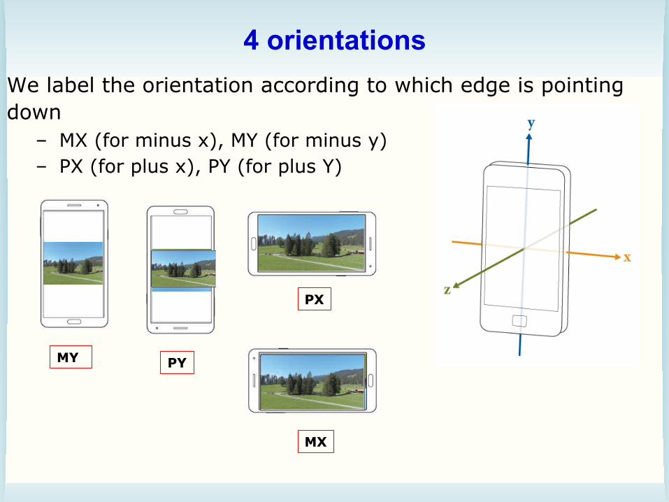
4 orientations We label the orientation according to which edge is pointing down
– MX (for minus x), MY (for minus y) – PX (for plus x), PY (for plus Y)
MY PY
PX
MX

Let us start simple
• We considered two orientations: MY and MX • We assumed the phone is vertical • We wanted to find a condition based on the
accelerations to classify the orientation – Basically a if-else statement, but what is the condition?
cond?
MY MX
MY
MX True False
This condition depends on the acceleration

Let us plot acceleration versus time
• Can you find some characteristics on the acceleration to differentiate between the orientations MX and MY?
ENGG1811 © UNSW, CRICOS Provider No: 00098G W9 slide 21

Plot y-acc versus x-acc
ENGG1811 © UNSW, CRICOS Provider No: 00098G W9 slide 22
• Orientation MX – x-acceleration big – y-acceleration small
• Orientation MY – x-acceleration small – y-acceleration big
Pseudo-code: If y-acc > x-acc
orientation MY else
orientation MX

A different perspective
ENGG1811 © UNSW, CRICOS Provider No: 00098G W9 slide 23
line x = y
y > x
x > y
Finding the Boolean expression is the same as finding a line that can separate the acceleration of different orientations into separate regions

Classify 4 orientations
• We want to classify 4 orientations • We no longer assume that the phone is vertical • Experiment
– Put the phone in each orientation – Tilt the phone but keeping one of +x, -x, +y, -y
down – Measure the acceleration in 3-directions
• Time plot on the next page
• Let us use 3D plot instead
ENGG1811 © UNSW, CRICOS Provider No: 00098G W9 slide 24

Time plot
ENGG1811 © UNSW, CRICOS Provider No: 00098G W9 slide 25
MY MY
PY PX
Matlab feature: subplot

Only need x- and y-acceleration
ENGG1811 © UNSW, CRICOS Provider No: 00098G W9 slide 26
The surprise is that acceleration in the z-direction is not needed at all!

ENGG1811 © UNSW, CRICOS Provider No: 00098G W9 slide 27
An exercise for you: boat hull*
A simple model for the hull of a boat is given by
where y is the width of the hull from the centre line, x is the distance along the centre line, and z is the depth of the hull. B is the beam (max width), L is the length and D is the draft (max depth). This hull is 8m long, with 3m beam and 1.5m draft.
* Based on Holloway, p.144 Project 15.
⎟⎟⎠
⎞⎜⎜⎝
⎛⎟⎠
⎞⎜⎝
⎛−⎟⎟⎠
⎞⎜⎜⎝
⎛⎟⎠
⎞⎜⎝
⎛−=22
1212 D
zLxBy

ENGG1811 © UNSW, CRICOS Provider No: 00098G W9 slide 28
Implementing the model
• x and z are the independent variables, and range from –L/2 to L/2, and –D to 0 respectively – use linspace and meshgrid to generate these arrays
• The first half of the y values (the starboard side) are produced by the formula, the second set of y values has the opposite sign – to display both halves (thus avoiding a massive maritime
disaster!), use the command hold on between plot commands
– axis equal maintains aspect ratio (uniform scales)
• You can try – use the 3D rotation tool to examine the shape – does mesh or surf give the better view? – experiment with shading (faceted, flat or interp)


