Download - Weka Sample
Assignment: 1 Artificial Neural Network
1 | P a g e
Group members and Data Sets
CSC/14/51 – Nursery Data set (page 02-09)
CSC/14/05 - Thyroid Disease Dataset (page 10-16)
CSC/14/22- Wine Data set (page 17-20)
Performance Analysis of Different classifiers on WEKA

Assignment: 1 Artificial Neural Network
2 | P a g e
Introduction
Gathered data sets are include valuable information and knowledge which is often hidden. Processing the huge data
and retrieving meaningful information from it is a difficult task. The aim of our work is to investigate the performance
of different classification methods using WEKA for different three dataset obtained from UCI data archive.
WEKA is an open source software which consists of a collection of machine learning algorithms for data mining tasks.
This assignment is to investigate the performance of different classification or clustering methods for a set of large
data set.
Materials and methods
We have used the popular, open-source data mining tool Weka (version 3.6.6) for this analysis. Three different data
sets have been used and the performance of a comprehensive set of classification algorithms (classifiers) has been
analyzed. The analysis has been performed on a Mac book pro with Intel® i5 CPU, 2.24 GHz Processor, OSX
Yosemite and 4.00 GB of RAM. The data sets have been chosen such that they differ in size, mainly in terms of the
number of attributes.
For this study the following
Data sets were used:
a) Nursery Database, which is developed to rank applications for nursery schools for providing certain facilities,
based on three factors.
Occupation of parents and child's nursery
Family structure and financial standing
social and health picture of the family
Under this study there was 12960 samples (instances) were analyzed against eight attributes which are,
parents : usual, pretentious, great_pret
has_nurs : proper, less_proper, improper, critical, very_crit
form : complete, completed, incomplete, foster
children : 1, 2, 3, more
housing : convenient, less_conv, critical
finance : convenient, inconv
social : non-prob, slightly_prob, problematic and
health : recommended, priority, not_recom.
Classifiers were used:
A total of five classification procedures have been used for this performance comparative study. The
classifiers in Weka have been categorized into different groups such as Bayes, Functions, Lazy, Rules, Tree
based classifiers etc. The following sections explain a brief about each of these procedures/algorithms.
i. Multilayer Perceptron: Multilayer Perceptron is a nonlinear classifier based on the Perceptron. A Multilayer
Perceptron (MLP) is a back propagation neural network with one or more layers between input and
output layer.
ii. A Support Vector Machine (SVM): SVM is a discriminative classifier formally defined by a separating hyper
plane. In other words, given labeled training data (supervised learning), the algorithm outputs an optimal
hyper plane which categorizes new examples.
iii. J48: The J48 algorithm is WEKA’s implementation of the C4.5 decision tree learner. The algorithm uses a
greedy technique to induce decision trees for classification and uses reduced-error pruning.
Assignment: 1 Artificial Neural Network
3 | P a g e
iv. IBk: IBk is a k-nearest-neighbor classifier that uses the same distance metric. k-NN is a type of instance
based learning or lazy learning where the function is only approximated locally and all computation is
deferred until classification. In this algorithm an object is classified by a majority vote of its neighbors.
v. Naive Bayesian: Naive Bayesian classifier is developed on bayes conditional probability rule used for
performing classification tasks, assuming attributes as statistically independent; the word Naive means
strong. All attributes of the data set are considered as independent and strong of each other.
Steps to apply classification techniques on data set and get result in Weka:
Step 1: Take the input dataset.
Step 2: Apply the classifier algorithm on the whole data set.
Step 3: Note the accuracy given by it and time required for execution.
Step 4: Repeat step 2 and 3 for different classification algorithms on different datasets.
Step 5: Compare the different accuracy provided by the dataset with different classification algorithms and
Identify the significant classification algorithm for particular dataset
Results and Discussion
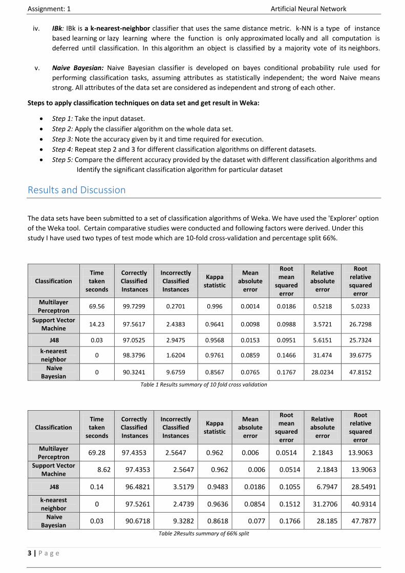
The data sets have been submitted to a set of classification algorithms of Weka. We have used the 'Explorer' option
of the Weka tool. Certain comparative studies were conducted and following factors were derived. Under this
study I have used two types of test mode which are 10-fold cross-validation and percentage split 66%.
Classification Time taken
seconds
Correctly Classified Instances
Incorrectly Classified Instances
Kappa statistic
Mean absolute
error
Root mean
squared error
Relative absolute
error
Root relative squared
error
Multilayer Perceptron
69.56 99.7299 0.2701 0.996 0.0014 0.0186 0.5218 5.0233
Support Vector Machine
14.23 97.5617 2.4383 0.9641 0.0098 0.0988 3.5721 26.7298
J48 0.03 97.0525 2.9475 0.9568 0.0153 0.0951 5.6151 25.7324
k-nearest neighbor
0 98.3796 1.6204 0.9761 0.0859 0.1466 31.474 39.6775
Naive Bayesian
0 90.3241 9.6759 0.8567 0.0765 0.1767 28.0234 47.8152
Table 1 Results summary of 10 fold cross validation
Classification Time taken
seconds
Correctly Classified Instances
Incorrectly Classified Instances
Kappa statistic
Mean absolute
error
Root mean
squared error
Relative absolute
error
Root relative squared
error
Multilayer Perceptron
69.28 97.4353 2.5647 0.962 0.006 0.0514 2.1843 13.9063
Support Vector Machine
8.62 97.4353 2.5647 0.962 0.006 0.0514 2.1843 13.9063
J48 0.14 96.4821 3.5179 0.9483 0.0186 0.1055 6.7947 28.5491
k-nearest neighbor
0 97.5261 2.4739 0.9636 0.0854 0.1512 31.2706 40.9314
Naive Bayesian
0.03 90.6718 9.3282 0.8618 0.077 0.1766 28.185 47.7877
Table 2Results summary of 66% split

Assignment: 1 Artificial Neural Network
4 | P a g e
0
20
40
60
80
MultilayerPerceptron
SupportVector
Machine
J48 k-nearestneighbor
NaiveBayesian
Time Taken in seconds
Cross validation 10 66% split
When considering time consuming for five classifiers
under two testing sample methods, the 66% split
take short time for SVM method of classification ,but
comparatively the cross validation method take
more time than percentage split.
8486889092949698
100102
MultilayerPerceptron
SupportVector
Machine
J48 k-nearestneighbor
NaiveBayesian
Correctly Classified Instances
Cross validation 10 66% split
Correctly identified instances are showing better
results under cross validation test mode. All together
all classifier shows relatively similar results except the
naive Bayesian classifier. It gives better results under
the 66% split test mode.
02468
1012
MultilayerPerceptron
SupportVector
Machine
J48 k-nearestneighbor
NaiveBayesian
Incorrectly Classified Instances
Cross validation 10 66% split
If we consider the incorrectly identified instances,
again the split validation shows poor performance
than cross validation test mode. Under multilayer
perception, the graph shows greater deviation from
each test mode and cross validation gives better
results under, the multilayer perception classifier.
The naïve Bayesian shows low performance in both
test mode.
0.750.8
0.850.9
0.951
1.05
MultilayerPerceptron
SupportVector
Machine
J48 k-nearestneighbor
NaiveBayesian
Capa Statistics
Cross validation 10 66% split
Capa statistics coefficient is a statistical measure of
inter-rater agreement or inter-annotator agreement
for qualitative (categorical) items. From capa we can
come to this conclusion.
< 0 Less than chance agreement
0.01–0.20 Slight agreement
0.21– 0.40 Fair agreement
0.41–0.60 Moderate agreement
0.61–0.80 Substantial agreement
0.81–0.99 Almost perfect agreement
0
0.02
0.04
0.06
0.08
0.1
MultilayerPerceptron
SupportVector
Machine
J48 k-nearestneighbor
NaiveBayesian
Mean absolute error
Cross validation 10 66% split
The MAE measures the average magnitude of the
errors in a set of five classes. If we consider the
following graph the k-nearest neighbor classifier
shows high mean absolute error than other classifier.
The multilayer perception shows relatively low
absolute error from others and J48 shows average
error rate. When considering the two training modes
there are no big deviation from each other except
the multilayer perception. Multilayer perception
shows low absolute error under cross validation
training mode.
Assignment: 1 Artificial Neural Network
5 | P a g e
0%10%20%30%40%50%60%70%80%90%
100%
Timetaken
seconds
CorrectlyClassified Instances
IncorrectlyClassifiedInstances
Kappastatistic
Meanabsolute
error
Root meansquared
error
Relativeabsolute
error
Root relativesquared
error
10-fold cross-validation
MultilayerPerceptron
SupportVectorMachine
J48 k-nearestneighbor
NaiveBayesian
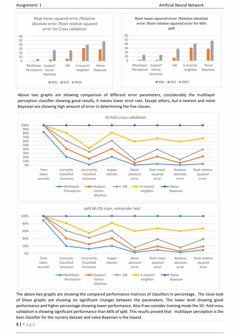
The above two graphs are showing the compared performance matrices of classifiers in percentage. The close look
of these graphs are showing no significant changes between the parameters. The lower level showing good
performance and higher percentage showing lower performance. Also if we consider training mode the 10 –fold cross
validation is showing significant performance than 66% of split. This results proved that multilayer perception is the
best classifier for the nursery dataset and naïve Bayesian is the lowest.
0102030405060
MultilayerPerceptron
SupportVector
Machine
J48 k-nearestneighbor
NaiveBayesian
Root mean squared error /Relative absolute error /Root relative squared
error for Cross validation
RMs RAE RRSE
0102030405060
MultilayerPerceptron
SupportVector
Machine
J48 k-nearestneighbor
NaiveBayesian
Root mean squared error /Relative absolute error /Root relative squared error for 66%
split
RMs RAE RRSE
Above two graphs are showing comparison of different error parameters, considerably the multilayer
perception classifier showing good results, it means lower error rate. Except others, but k-nearest and naïve
Bayesian are showing high amount of error in determining the five classes.
0%
20%
40%
60%
80%
100%
Timetaken
seconds
CorrectlyClassified Instances
IncorrectlyClassifiedInstances
Kappastatistic
Meanabsolute
error
Root meansquared
error
Relativeabsolute
error
Root relativesquared
error
split 66.0% train, remainder test
MultilayerPerceptron
SupportVectorMachine
J48 k-nearestneighbor
NaiveBayesian

Assignment: 1 Artificial Neural Network
6 | P a g e
0
0.2
0.4
0.6
0.8
1
1.2
MultilayerPerceptron
SupportVector
Machine
J48 k-nearestneighbor
NaiveBayesian
TP Rate Cross Validation
not_recom recommend very_recom
priority spec_prior
0
0.2
0.4
0.6
0.8
1
1.2
MultilayerPerceptron
SupportVector
Machine
J48 k-nearestneighbor
NaiveBayesian
TP Rate for % split
not_recom recommend very_recom
priority spec_prior
The above graphs are showing the precision comparison of five classifier against five classes that we have identified.
Under cross validation training mode the class recommended shows zero precision among all classifier we have used.
But class not_recommeded shows high precision in both training mode. But ver_recommeded class show significant
precision in 66% split. Considering above fact the cross validation again lead in performance.
Considering the True positive rate the not recommended class is showing similar results under both testing mode
and all types of classifier used same like us the priority and specific priority class. But the class very recommended is
showing significant different between classifiers and testing mode. However we got good results in multilayer
perception and J48 under cross validation testing mode.
0
0.002
0.004
0.006
0.008
0.01
0.012
MultilayerPerceptron
SupportVector
Machine
J48 k-nearestneighbor
NaiveBayesian
HU
ND
RED
SPrecision of c lassifiers (Cross
Validation)
not_recom recommend very_recom
priority spec_prior
0
0.002
0.004
0.006
0.008
0.01
0.012
MultilayerPerceptron
SupportVector
Machine
J48 k-nearestneighbor
NaiveBayesian
HU
ND
RED
S
Precision of classifiers (66% split)
not_recom recommend very_recom
priority spec_prior
0
0.02
0.04
0.06
0.08
0.1
0.12
MultilayerPerceptron
SupportVector
Machine
J48 k-nearestneighbor
NaiveBayesian
FP Rate Cross Validation
not_recom recommend very_recom
priority spec_prior
0
0.02
0.04
0.06
0.08
0.1
MultilayerPerceptron
SupportVector
Machine
J48 k-nearestneighbor
NaiveBayesian
FP Rate for % split
not_recom recommend very_recom
priority spec_prior
Assignment: 1 Artificial Neural Network
7 | P a g e
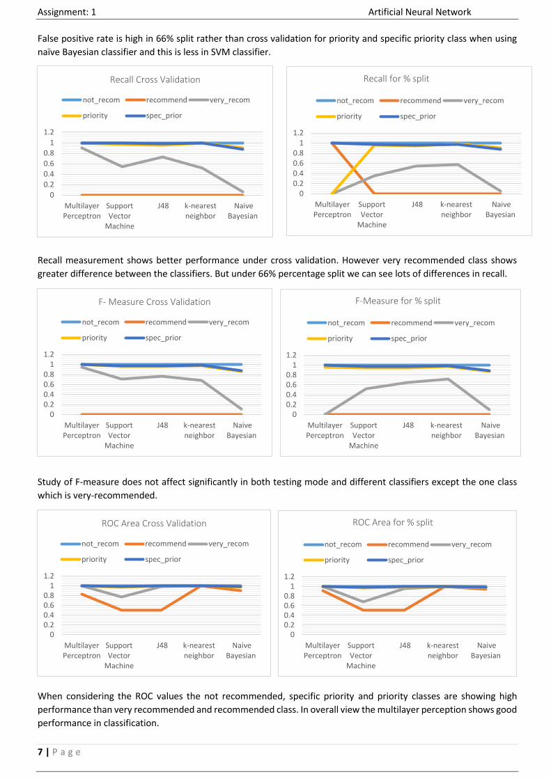
False positive rate is high in 66% split rather than cross validation for priority and specific priority class when using
naïve Bayesian classifier and this is less in SVM classifier.
Recall measurement shows better performance under cross validation. However very recommended class shows
greater difference between the classifiers. But under 66% percentage split we can see lots of differences in recall.
Study of F-measure does not affect significantly in both testing mode and different classifiers except the one class
which is very-recommended.
When considering the ROC values the not recommended, specific priority and priority classes are showing high
performance than very recommended and recommended class. In overall view the multilayer perception shows good
performance in classification.
0
0.2
0.4
0.6
0.8
1
1.2
MultilayerPerceptron
SupportVector
Machine
J48 k-nearestneighbor
NaiveBayesian
Recall Cross Validation
not_recom recommend very_recom
priority spec_prior
00.20.40.60.8
11.2
MultilayerPerceptron
SupportVector
Machine
J48 k-nearestneighbor
NaiveBayesian
Recall for % split
not_recom recommend very_recom
priority spec_prior
00.20.40.60.8
11.2
MultilayerPerceptron
SupportVector
Machine
J48 k-nearestneighbor
NaiveBayesian
F- Measure Cross Validation
not_recom recommend very_recom
priority spec_prior
00.20.40.60.8
11.2
MultilayerPerceptron
SupportVector
Machine
J48 k-nearestneighbor
NaiveBayesian
F-Measure for % split
not_recom recommend very_recom
priority spec_prior
00.20.40.60.8
11.2
MultilayerPerceptron
SupportVector
Machine
J48 k-nearestneighbor
NaiveBayesian
ROC Area Cross Validation
not_recom recommend very_recom
priority spec_prior
00.20.40.60.8
11.2
MultilayerPerceptron
SupportVector
Machine
J48 k-nearestneighbor
NaiveBayesian
ROC Area for % split
not_recom recommend very_recom
priority spec_prior

Assignment: 1 Artificial Neural Network
8 | P a g e
ROC curve Analysis
To analyze the ROC performance the above model was developed.by running the model ROC curves were obtained
for different classifiers of particular class.
Class: - not recommended Class :- recommended
Class: - Very recommended Class: - priority
When seeing the above ROC curves of classes the recommended class shows poor performance for most of the
classifiers. May due to less amount of instances in that class. (Depend on the data set). Most of the time multilayer
perception gives the good performance. The analysis of ROC time consuming process therefore I did only for cross
validation mode.
Assignment: 1 Artificial Neural Network
9 | P a g e
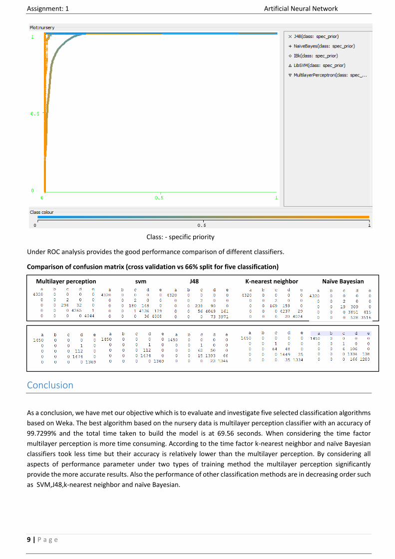
Class: - specific priority
Under ROC analysis provides the good performance comparison of different classifiers.
Comparison of confusion matrix (cross validation vs 66% split for five classification)
Multilayer perception svm J48 K-nearest neighbor Naïve Bayesian
Conclusion
As a conclusion, we have met our objective which is to evaluate and investigate five selected classification algorithms
based on Weka. The best algorithm based on the nursery data is multilayer perception classifier with an accuracy of
99.7299% and the total time taken to build the model is at 69.56 seconds. When considering the time factor
multilayer perception is more time consuming. According to the time factor k-nearest neighbor and naïve Bayesian
classifiers took less time but their accuracy is relatively lower than the multilayer perception. By considering all
aspects of performance parameter under two types of training method the multilayer perception significantly
provide the more accurate results. Also the performance of other classification methods are in decreasing order such
as SVM,J48,k-nearest neighbor and naïve Bayesian.
Assignment: 1 Artificial Neural Network
10 | P a g e
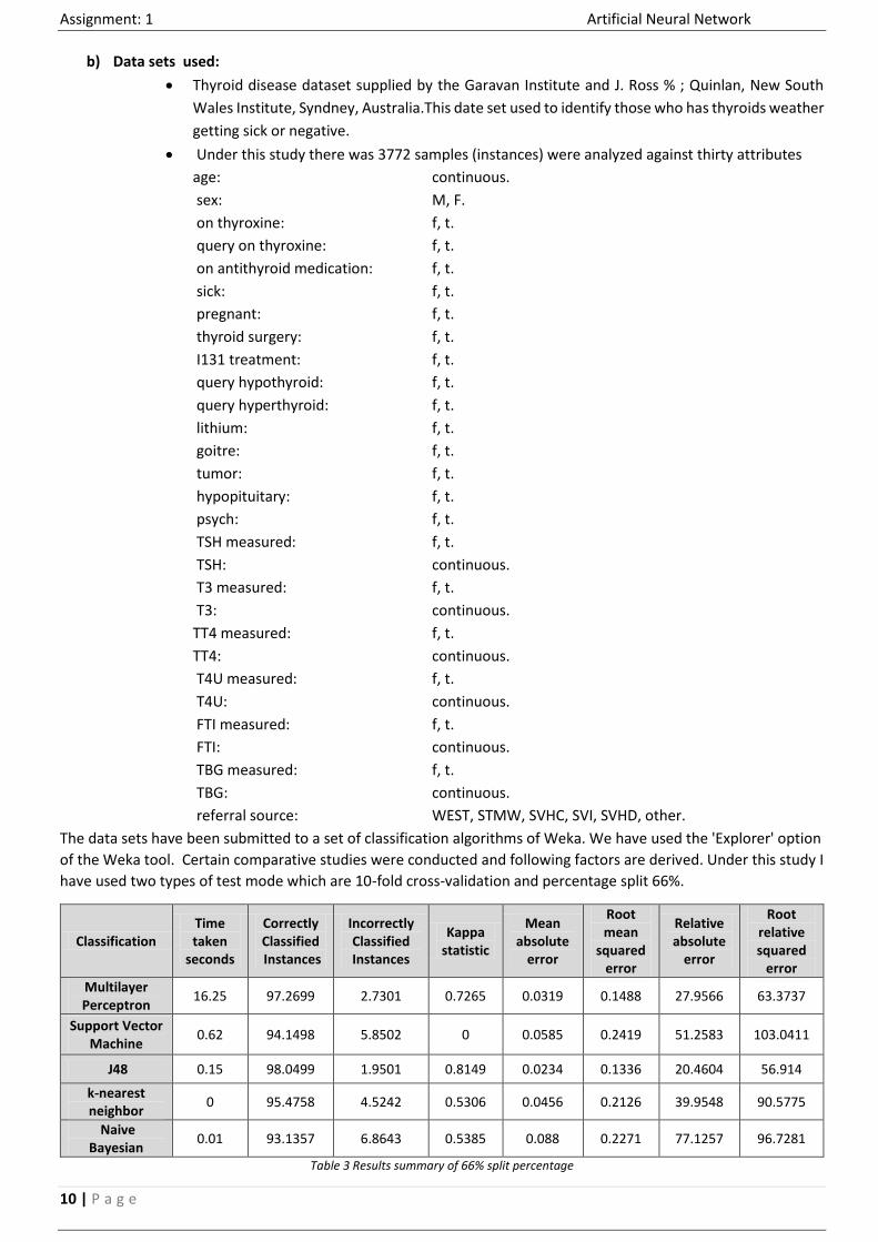
b) Data sets used:
Thyroid disease dataset supplied by the Garavan Institute and J. Ross % ; Quinlan, New South
Wales Institute, Syndney, Australia.This date set used to identify those who has thyroids weather
getting sick or negative.
Under this study there was 3772 samples (instances) were analyzed against thirty attributes
age: continuous.
sex: M, F.
on thyroxine: f, t.
query on thyroxine: f, t.
on antithyroid medication: f, t.
sick: f, t.
pregnant: f, t.
thyroid surgery: f, t.
I131 treatment: f, t.
query hypothyroid: f, t.
query hyperthyroid: f, t.
lithium: f, t.
goitre: f, t.
tumor: f, t.
hypopituitary: f, t.
psych: f, t.
TSH measured: f, t.
TSH: continuous.
T3 measured: f, t.
T3: continuous.
TT4 measured: f, t.
TT4: continuous.
T4U measured: f, t.
T4U: continuous.
FTI measured: f, t.
FTI: continuous.
TBG measured: f, t.
TBG: continuous.
referral source: WEST, STMW, SVHC, SVI, SVHD, other.
The data sets have been submitted to a set of classification algorithms of Weka. We have used the 'Explorer' option
of the Weka tool. Certain comparative studies were conducted and following factors are derived. Under this study I
have used two types of test mode which are 10-fold cross-validation and percentage split 66%.
Classification Time taken
seconds
Correctly Classified Instances
Incorrectly Classified Instances
Kappa statistic
Mean absolute
error
Root mean
squared error
Relative absolute
error
Root relative squared
error
Multilayer Perceptron
16.25 97.2699 2.7301 0.7265 0.0319 0.1488 27.9566 63.3737
Support Vector Machine
0.62 94.1498 5.8502 0 0.0585 0.2419 51.2583 103.0411
J48 0.15 98.0499 1.9501 0.8149 0.0234 0.1336 20.4604 56.914
k-nearest neighbor
0 95.4758 4.5242 0.5306 0.0456 0.2126 39.9548 90.5775
Naive Bayesian
0.01 93.1357 6.8643 0.5385 0.088 0.2271 77.1257 96.7281
Table 3 Results summary of 66% split percentage
Assignment: 1 Artificial Neural Network
11 | P a g e
Classification Time taken
seconds
Correctly Classified Instances
Incorrectly Classified Instances
Kappa statistic
Mean absolute
error
Root mean
squared error
Relative absolute
error
Root relative squared
error
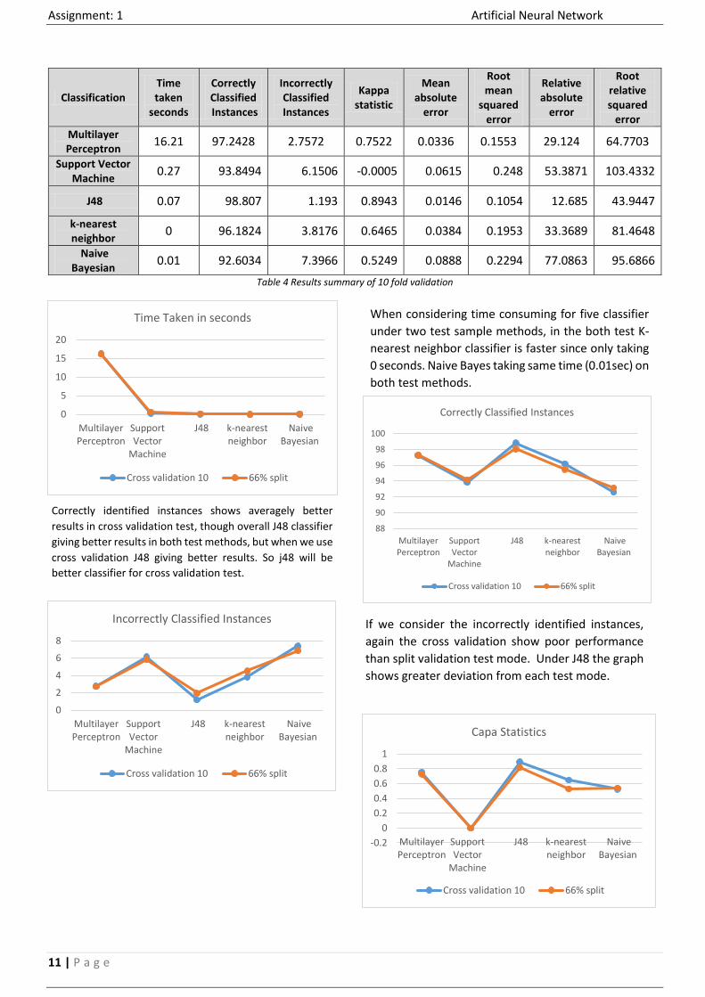
Multilayer Perceptron
16.21 97.2428 2.7572 0.7522 0.0336 0.1553 29.124 64.7703
Support Vector Machine
0.27 93.8494 6.1506 -0.0005 0.0615 0.248 53.3871 103.4332
J48 0.07 98.807 1.193 0.8943 0.0146 0.1054 12.685 43.9447
k-nearest neighbor
0 96.1824 3.8176 0.6465 0.0384 0.1953 33.3689 81.4648
Naive Bayesian
0.01 92.6034 7.3966 0.5249 0.0888 0.2294 77.0863 95.6866
Table 4 Results summary of 10 fold validation
0
5
10
15
20
MultilayerPerceptron
SupportVector
Machine
J48 k-nearestneighbor
NaiveBayesian
Time Taken in seconds
Cross validation 10 66% split
When considering time consuming for five classifier
under two test sample methods, in the both test K-
nearest neighbor classifier is faster since only taking
0 seconds. Naive Bayes taking same time (0.01sec) on
both test methods.
88
90
92
94
96
98
100
MultilayerPerceptron
SupportVector
Machine
J48 k-nearestneighbor
NaiveBayesian
Correctly Classified Instances
Cross validation 10 66% split
Correctly identified instances shows averagely better
results in cross validation test, though overall J48 classifier
giving better results in both test methods, but when we use
cross validation J48 giving better results. So j48 will be
better classifier for cross validation test.
0
2
4
6
8
MultilayerPerceptron
SupportVector
Machine
J48 k-nearestneighbor
NaiveBayesian
Incorrectly Classified Instances
Cross validation 10 66% split
If we consider the incorrectly identified instances,
again the cross validation show poor performance
than split validation test mode. Under J48 the graph
shows greater deviation from each test mode.
-0.2
0
0.2
0.4
0.6
0.8
1
MultilayerPerceptron
SupportVector
Machine
J48 k-nearestneighbor
NaiveBayesian
Capa Statistics
Cross validation 10 66% split
Assignment: 1 Artificial Neural Network
12 | P a g e
0%
10%
20%
30%
40%
50%
60%
70%
80%
90%
100%
Timetaken
seconds
CorrectlyClassified Instances
IncorrectlyClassifiedInstances
Kappastatistic
Meanabsolute
error
Root meansquared
error
Relativeabsolute
error
Root relativesquared
error
10-fold cross-validation
MultilayerPerceptron
SupportVectorMachine
J48 k-nearestneighbor
NaiveBayesian
0
0.02
0.04
0.06
0.08
0.1
MultilayerPerceptron
SupportVector
Machine
J48 k-nearestneighbor
NaiveBayesian
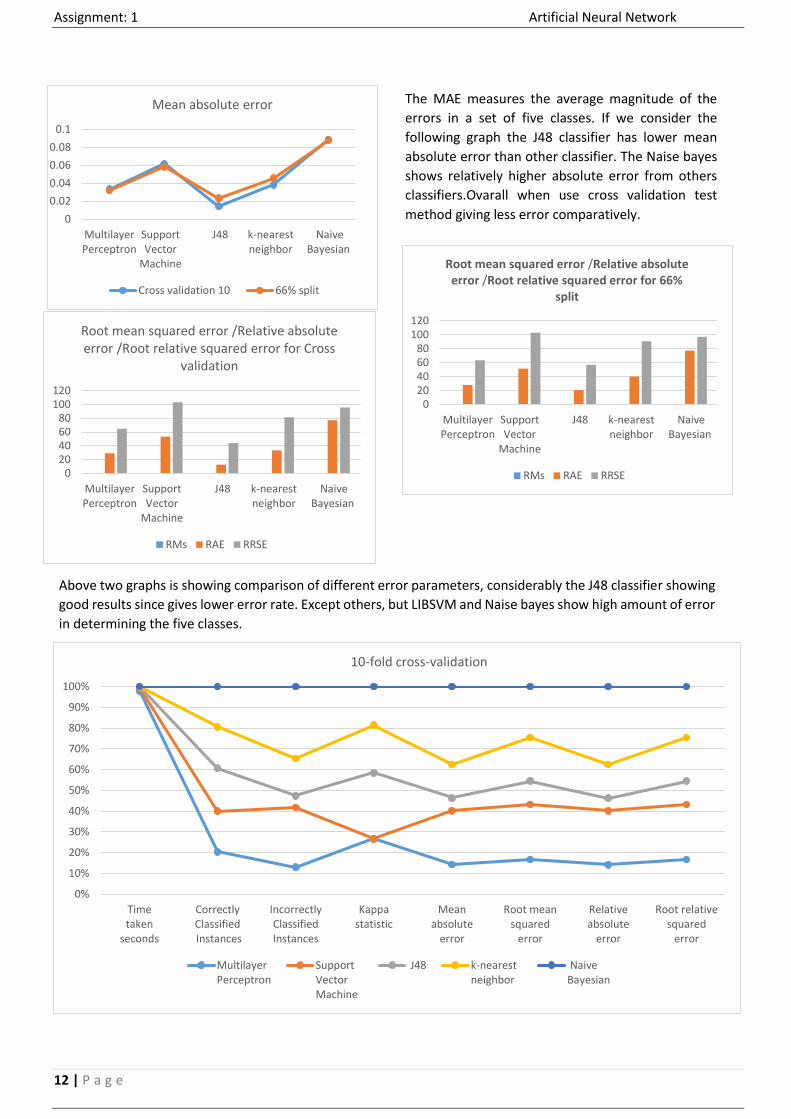
Mean absolute error
Cross validation 10 66% split
The MAE measures the average magnitude of the
errors in a set of five classes. If we consider the
following graph the J48 classifier has lower mean
absolute error than other classifier. The Naise bayes
shows relatively higher absolute error from others
classifiers.Ovarall when use cross validation test
method giving less error comparatively.
020406080
100120
MultilayerPerceptron
SupportVector
Machine
J48 k-nearestneighbor
NaiveBayesian
Root mean squared error /Relative absolute error /Root relative squared error for Cross
validation
RMs RAE RRSE
020406080
100120
MultilayerPerceptron
SupportVector
Machine
J48 k-nearestneighbor
NaiveBayesian
Root mean squared error /Relative absolute error /Root relative squared error for 66%
split
RMs RAE RRSE
Above two graphs is showing comparison of different error parameters, considerably the J48 classifier showing
good results since gives lower error rate. Except others, but LIBSVM and Naise bayes show high amount of error
in determining the five classes.
Assignment: 1 Artificial Neural Network
13 | P a g e
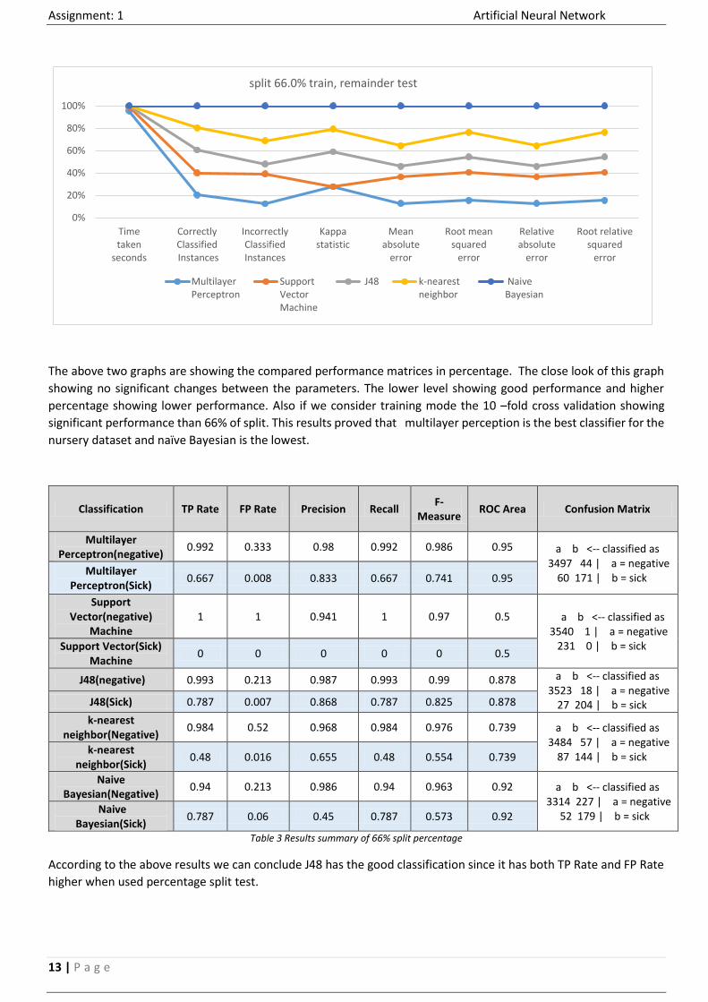
The above two graphs are showing the compared performance matrices in percentage. The close look of this graph
showing no significant changes between the parameters. The lower level showing good performance and higher
percentage showing lower performance. Also if we consider training mode the 10 –fold cross validation showing
significant performance than 66% of split. This results proved that multilayer perception is the best classifier for the
nursery dataset and naïve Bayesian is the lowest.
Classification TP Rate FP Rate Precision Recall F-
Measure ROC Area Confusion Matrix
Multilayer Perceptron(negative)
0.992 0.333 0.98 0.992 0.986 0.95 a b <-- classified as 3497 44 | a = negative 60 171 | b = sick
Multilayer Perceptron(Sick)
0.667 0.008 0.833 0.667 0.741 0.95
Support Vector(negative)
Machine 1 1 0.941 1 0.97 0.5 a b <-- classified as
3540 1 | a = negative 231 0 | b = sick Support Vector(Sick)
Machine 0 0 0 0 0 0.5
J48(negative) 0.993 0.213 0.987 0.993 0.99 0.878 a b <-- classified as 3523 18 | a = negative 27 204 | b = sick J48(Sick) 0.787 0.007 0.868 0.787 0.825 0.878
k-nearest neighbor(Negative)
0.984 0.52 0.968 0.984 0.976 0.739 a b <-- classified as 3484 57 | a = negative 87 144 | b = sick
k-nearest neighbor(Sick)
0.48 0.016 0.655 0.48 0.554 0.739
Naive Bayesian(Negative)
0.94 0.213 0.986 0.94 0.963 0.92 a b <-- classified as 3314 227 | a = negative 52 179 | b = sick
Naive Bayesian(Sick)
0.787 0.06 0.45 0.787 0.573 0.92
Table 3 Results summary of 66% split percentage
According to the above results we can conclude J48 has the good classification since it has both TP Rate and FP Rate
higher when used percentage split test.
0%
20%
40%
60%
80%
100%
Timetaken
seconds
CorrectlyClassified Instances
IncorrectlyClassifiedInstances
Kappastatistic
Meanabsolute
error
Root meansquared
error
Relativeabsolute
error
Root relativesquared
error
split 66.0% train, remainder test
MultilayerPerceptron
SupportVectorMachine
J48 k-nearestneighbor
NaiveBayesian
Assignment: 1 Artificial Neural Network
14 | P a g e
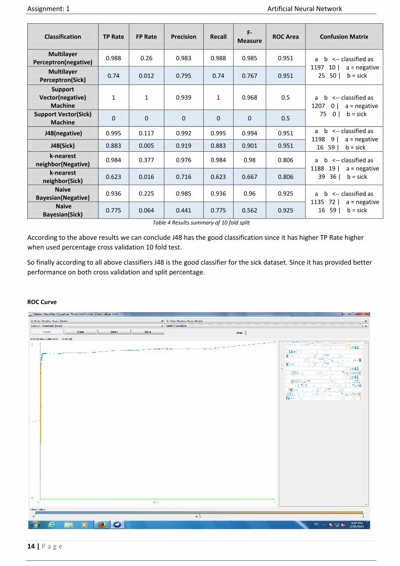
Classification TP Rate FP Rate Precision Recall F-
Measure ROC Area Confusion Matrix
Multilayer Perceptron(negative)
0.988 0.26 0.983 0.988 0.985 0.951 a b <-- classified as 1197 10 | a = negative 25 50 | b = sick
Multilayer Perceptron(Sick)
0.74 0.012 0.795 0.74 0.767 0.951
Support Vector(negative)
Machine 1 1 0.939 1 0.968 0.5 a b <-- classified as
1207 0 | a = negative 75 0 | b = sick Support Vector(Sick)
Machine 0 0 0 0 0 0.5
J48(negative) 0.995 0.117 0.992 0.995 0.994 0.951 a b <-- classified as 1198 9 | a = negative 16 59 | b = sick J48(Sick) 0.883 0.005 0.919 0.883 0.901 0.951
k-nearest neighbor(Negative)
0.984 0.377 0.976 0.984 0.98 0.806 a b <-- classified as 1188 19 | a = negative 39 36 | b = sick
k-nearest neighbor(Sick)
0.623 0.016 0.716 0.623 0.667 0.806
Naive Bayesian(Negative)
0.936 0.225 0.985 0.936 0.96 0.925 a b <-- classified as 1135 72 | a = negative 16 59 | b = sick
Naive Bayesian(Sick)
0.775 0.064 0.441 0.775 0.562 0.925
Table 4 Results summary of 10 fold split
According to the above results we can conclude J48 has the good classification since it has higher TP Rate higher
when used percentage cross validation 10 fold test.
So finally according to all above classifiers J48 is the good classifier for the sick dataset. Since it has provided better
performance on both cross validation and split percentage.
ROC Curve

Assignment: 1 Artificial Neural Network
15 | P a g e
Fig1 ROC curve for J48 (cross validation-fold 10)
Fig2 ROC curve for J48 (percentage split)
Assignment: 1 Artificial Neural Network
16 | P a g e
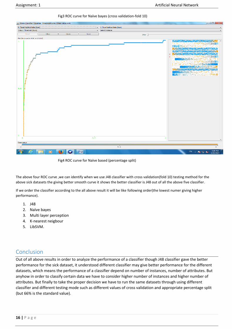
Fig3 ROC curve for Naïve bayes (cross validation-fold 10)
Fig4 ROC curve for Naïve based (percentage split)
The above four ROC curve ,we can identify when we use J48 classifier with cross validation(fold 10) testing method for the
above sick datasets the giving better smooth curve it shows the better classifier is J48 out of all the above five classifier.
If we order the classifier according to the all above result it will be like following order(the lowest numer giving higher
performance).
1. J48
2. Naïve bayes
3. Multi layer perception
4. K-nearest neigbour
5. LibSVM.
Conclusion Out of all above results in order to analyze the performance of a classifier though J48 classifier gave the better
performance for the sick dataset, it understood different classifier may give better performance for the different
datasets, which means the performance of a classifier depend on number of instances, number of attributes. But
anyhow in order to classify certain data we have to consider higher number of instances and higher number of
attributes. But finally to take the proper decision we have to run the same datasets through using different
classifier and different testing mode such as different values of cross validation and appropriate percentage split
(but 66% is the standard value).
Assignment: 1 Artificial Neural Network
17 | P a g e
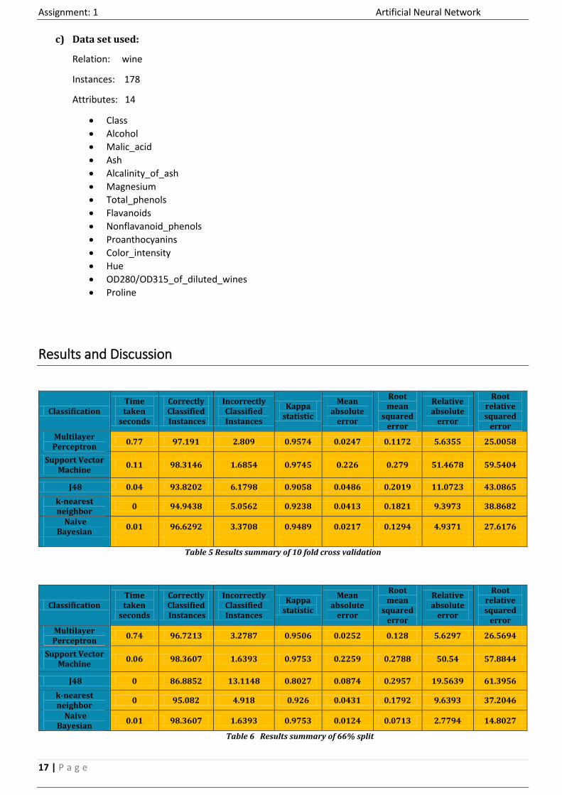
c) Data set used:
Relation: wine
Instances: 178
Attributes: 14
Class
Alcohol
Malic_acid
Ash
Alcalinity_of_ash
Magnesium
Total_phenols
Flavanoids
Nonflavanoid_phenols
Proanthocyanins
Color_intensity
Hue
OD280/OD315_of_diluted_wines
Proline
Results and Discussion
Table 5 Results summary of 10 fold cross validation
Classification Time taken
seconds
Correctly Classified Instances
Incorrectly Classified Instances
Kappa statistic
Mean absolute
error
Root mean
squared error
Relative absolute
error
Root relative squared
error Multilayer Perceptron
0.74 96.7213 3.2787 0.9506 0.0252 0.128 5.6297 26.5694
Support Vector Machine
0.06 98.3607 1.6393 0.9753 0.2259 0.2788 50.54 57.8844
J48 0 86.8852 13.1148 0.8027 0.0874 0.2957 19.5639 61.3956
k-nearest neighbor
0 95.082 4.918 0.926 0.0431 0.1792 9.6393 37.2046
Naive Bayesian
0.01 98.3607 1.6393 0.9753 0.0124 0.0713 2.7794 14.8027
Table 6 Results summary of 66% split
Classification Time taken
seconds
Correctly Classified Instances
Incorrectly Classified Instances
Kappa statistic
Mean absolute
error
Root mean
squared error
Relative absolute
error
Root relative squared
error Multilayer Perceptron
0.77 97.191 2.809 0.9574 0.0247 0.1172 5.6355 25.0058
Support Vector Machine
0.11 98.3146 1.6854 0.9745 0.226 0.279 51.4678 59.5404
J48 0.04 93.8202 6.1798 0.9058 0.0486 0.2019 11.0723 43.0865
k-nearest neighbor
0 94.9438 5.0562 0.9238 0.0413 0.1821 9.3973 38.8682
Naive Bayesian
0.01 96.6292 3.3708 0.9489 0.0217 0.1294 4.9371 27.6176
Assignment: 1 Artificial Neural Network
18 | P a g e
00.10.20.30.40.50.60.70.80.9
MultilayerPerceptron
SupportVector
Machine
J48 k-nearestneighbor
NaiveBayesian
Time Taken in seconds
Cross validation 10 66% split
80
85
90
95
100
MultilayerPerceptron
SupportVector
Machine
J48 k-nearestneighbor
NaiveBayesian
Correctly Classified Instances
Cross validation 10 66% split
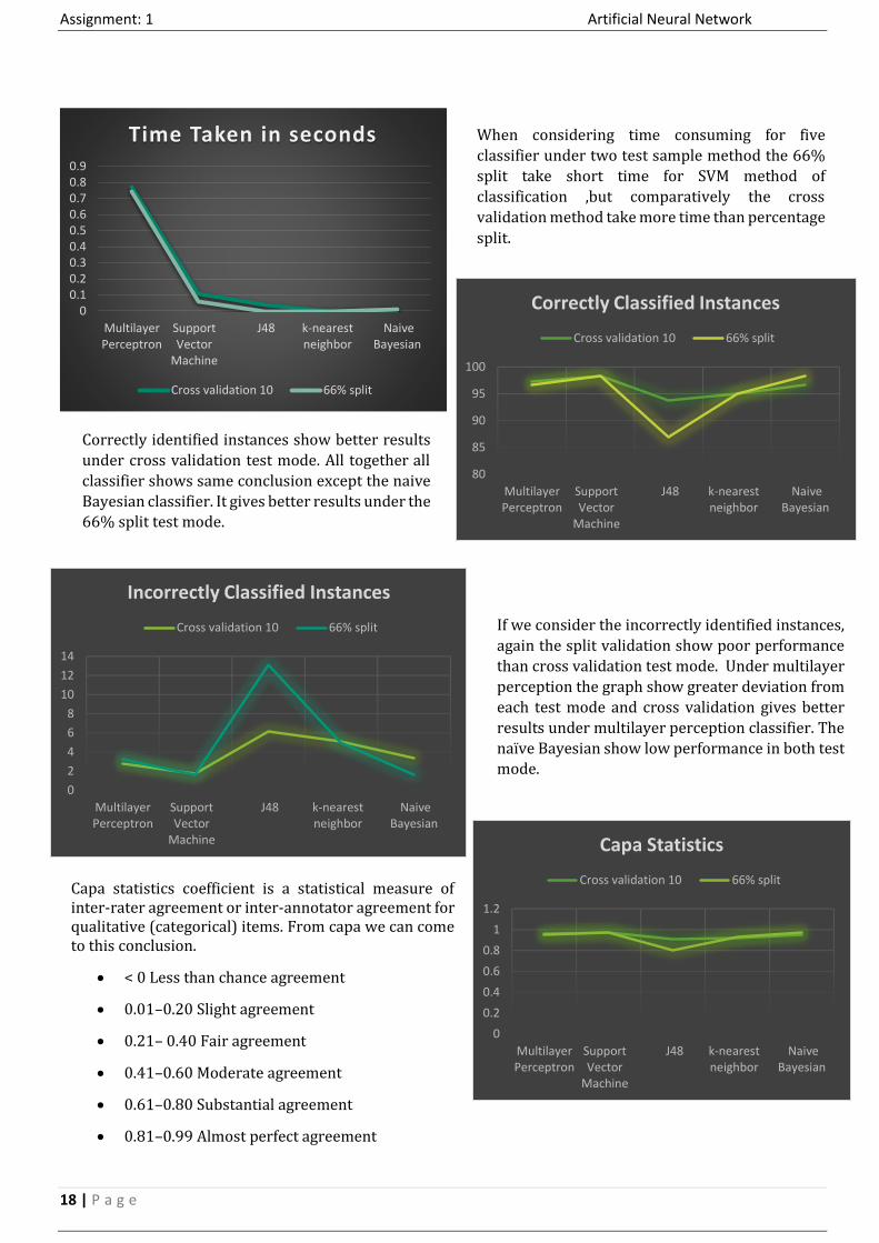
When considering time consuming for five
classifier under two test sample method the 66%
split take short time for SVM method of
classification ,but comparatively the cross
validation method take more time than percentage
split.
Correctly identified instances show better results
under cross validation test mode. All together all
classifier shows same conclusion except the naive
Bayesian classifier. It gives better results under the 66% split test mode.
0
2
4
6
8
10
12
14
MultilayerPerceptron
SupportVector
Machine
J48 k-nearestneighbor
NaiveBayesian
Incorrectly Classified Instances
Cross validation 10 66% split
0
0.2
0.4
0.6
0.8
1
1.2
MultilayerPerceptron
SupportVector
Machine
J48 k-nearestneighbor
NaiveBayesian
Capa Statistics
Cross validation 10 66% split
If we consider the incorrectly identified instances,
again the split validation show poor performance
than cross validation test mode. Under multilayer
perception the graph show greater deviation from
each test mode and cross validation gives better
results under multilayer perception classifier. The
naïve Bayesian show low performance in both test mode.
.
Capa statistics coefficient is a statistical measure of inter-rater agreement or inter-annotator agreement for qualitative (categorical) items. From capa we can come to this conclusion.
< 0 Less than chance agreement
0.01–0.20 Slight agreement
0.21– 0.40 Fair agreement
0.41–0.60 Moderate agreement
0.61–0.80 Substantial agreement
0.81–0.99 Almost perfect agreement

Assignment: 1 Artificial Neural Network
19 | P a g e
0
0.05
0.1
0.15
0.2
0.25
MultilayerPerceptron
SupportVector
Machine
J48 k-nearestneighbor
NaiveBayesian
Mean absolute error
Cross validation 10 66% split
0.1172 0.279 0.2019 0.1821 0.12945.6355
51.4678
11.0723 9.39734.9371
25.0058
59.5404
43.086538.8682
27.6176
0
10
20
30
40
50
60
70
MultilayerPerceptron
SupportVector
Machine
J48 k-nearestneighbor
NaiveBayesian
Root mean squared error /Relative absolute error /Root relative squared error for Cross validation
RMs RAE RRSE
0.128 0.2788 0.2957 0.1792 0.07135.6297
50.54
19.5639
9.63932.7794
25.5694
57.884461.3956
37.2046
14.8027
0
10
20
30
40
50
60
70
MultilayerPerceptron
SupportVector
Machine
J48 k-nearestneighbor
NaiveBayesian
Root mean squared error /Relative absolute error /Root relative squared error for 66% split
RMs RAE RRSE
The MAE measures the average magnitude of the errors in a set of five classes. If we consider the following graph the Support vector machine classifier shows high mean absolute error than other classifier. The multilayer perception shows relatively low absolute error from others and J48 shows average error rate. When considering the two train modes there is no big deviation from each other except the multilayer perception. Multilayer perception shows low absolute error under cross validation training mode.
Above two graphs are showing comparison of different error parameters, considerably the multilayer
perception classifier showing good results that means lower error rate. Except others, but Support vector Machine and J48 show high amount of error in determining the five classes.
Assignment: 1 Artificial Neural Network
20 | P a g e
0%
20%
40%
60%
80%
100%
Timetaken
seconds
CorrectlyClassified Instances
IncorrectlyClassifiedInstances
Kappastatistic
Meanabsolute
error
Root meansquared
error
Relativeabsolute
error
Root relativesquared
error
10-fold Cross-Validation
MultilayerPerceptron
SupportVectorMachine
J48 k-nearestneighbor
NaiveBayesian
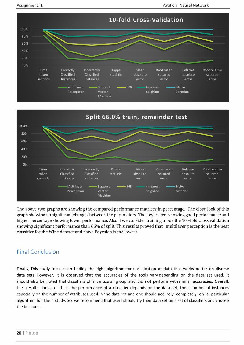
The above two graphs are showing the compared performance matrices in percentage. The close look of this
graph showing no significant changes between the parameters. The lower level showing good performance and
higher percentage showing lower performance. Also if we consider training mode the 10 –fold cross validation
showing significant performance than 66% of split. This results proved that multilayer perception is the best classifier for the Wine dataset and naïve Bayesian is the lowest.
Final Conclusion
Finally, This study focuses on finding the right algorithm for classification of data that works better on diverse
data sets. However, it is observed that the accuracies of the tools vary depending on the data set used. It
should also be noted that classifiers of a particular group also did not perform with similar accuracies. Overall,
the results indicate that the performance of a classifier depends on the data set, then number of instances
especially on the number of attributes used in the data set and one should not rely completely on a particular
algorithm for their study. So, we recommend that users should try their data set on a set of classifiers and choose
the best one.
0%
20%
40%
60%
80%
100%
Timetaken
seconds
CorrectlyClassified Instances
IncorrectlyClassifiedInstances
Kappastatistic
Meanabsolute
error
Root meansquared
error
Relativeabsolute
error
Root relativesquared
error
Split 66.0% train, remainder test
MultilayerPerceptron
SupportVectorMachine
J48 k-nearestneighbor
NaiveBayesian

Assignment: 1 Artificial Neural Network
21 | P a g e
References
1. Gopala Krishna, Bharath Kumar and Nagaraju Orsu “Performance Analysis and Evaluation of Different Data
Mining Algorithms used for Cancer Classification”, (IJARAI) International Journal of Advanced Research in
Artificial Intelligence, Vol. 2, No.5, 2013.
2. Mohd Fauzi bin Othman and Thomas Moh Shan Yau “Comparison of Different Classification Techniques
Using WEKA for Breast Cancer” IFMBE Proceedings Vol. 15.2007.
3. Rohit Arora and Suman “Comparative Analysis of Classification Algorithms onDifferent Datasets using
WEKA”, International Journal of Computer Applications (0975 – 8887),Volume 54– No.13, September 2012
4. Samrat Singh and Vikesh Kumar ” Performance Analysis of Engineering Students for Recruitment Using
Classification Data Mining Techniques” Samrat Singh et al , IJCSET , Vol 3, Issue 2, 31-37 ,February 2013 .


