
Working Paper Series No 66 / January 2018
How effective are sovereign bond-backed securities as a spillover prevention device? by David Cronin Peter G. Dunne

Abstract
Brunnermeier et al. (2017) propose the introduction of sovereign bond-backed securities
(SBBS) in the euro area. That and other papers assess how the securitisation would
insulate senior bond holders from actual default-related losses. This paper generalises
the assessment by using the VAR-based Diebold and Yilmaz (2012) spillover index
methodology to assess potential attenuation of the spillover of shocks in holding-period
returns across bond markets due to the introduction of SBBS. This is made possible by
employing SBBS yields estimated from historical euro area member state sovereign bond
yields using Monte Carlo methods, as described in Schonbucher (2003). A lower spillover
of shocks between SBBS securities compared to what arises between eleven member states’
bond markets is observed. Spillover values fall during the euro area sovereign bond crisis.
Gross and net spillovers are lower for a 70-30 tranching than for a 70-20-10 case but in
both cases the senior tranche becomes more insulated from shocks in the more junior
tranches during periods of financial stress.
Keywords: Safe Assets; Sovereign Bond Securitisation; Bank-Sovereign Diabolic Loop
JEL: C58, G11, G12, G17.

2
1. Introduction
Brunnermeier et al. (2016) and Brunnermeier et al. (2017) propose the issuance
of sovereign bond-backed securities (SBBS) in the euro area with tranches
that would be sequentially exposed to losses arising from any defaults on the
underlying individual sovereign securities. One of the principal motivations for
this proposal is to reduce the potential for spillovers across sovereign bond
markets owing to localised shocks. The authors argue that, in doing so, this
initiative also has the potential to reduce self-fulfilling crisis dynamics within
euro area sovereign bond markets as has been argued to have happened in the
earlier years of this decade by De Grauwe and Ji (2013).
By definition, any securitisation that allocates default losses to subordinated
tranches will tend to protect some investors and increase the exposures of others
in the event of actual defaults.1 However, actual default events are rare and it
is the changing expectations of such events that affects investment returns in
advance of, and even in the absence of, eventual defaults. The focus in this paper
is therefore on the extent to which securitisation in the euro area sovereign
bond markets could reduce the spillover of shocks from one asset market to
another. Spillover effects are important since they have endogenous knock-on
effects to risk taking and investment behaviour. If a large fraction of existing
1. Indeed, simulated default exercises by Brunnermeier et al. (2017) show that, interms of default loss exposures, senior bonds in sovereign bond securitisations are ex postfundamentally safer than any existing individual sovereign while the mezzanine and juniortranches should experience expected loss rates comparable to those of euro area sovereignswith intermediate and extreme credit risks respectively.
3
sovereign securities in the euro area were to be replaced with less interconnected
assets (i.e. SBBS) then this will likely have implications for market resilience
to localised shocks.2 The Diebold and Yilmaz (2012) spillover index approach
allows a comparison of the interconnectedness of SBBS tranches to be made
with that among national sovereign bond markets within the euro area. The
analytical output it provides complements and adds to that of Brunnermeier
et al. (2016) and Brunnermeier et al. (2017) where the attenuation of default
loss exposure as a result of SBBS is assessed.
Identifying ways of significantly reducing risk exposures and spillovers in
financial markets is attractive to issuers and investors alike as doing so can
avoid conditions that result in actual defaults, including by a direct self-
fulfilling causal connection between market-based losses and default losses.
This is particularly important in euro area sovereign bond markets given the
stress and associated inter-market-related effects experienced in the early years
of this decade. Market-based exposures and interdependencies are labeled as
endogenous risk by Danielsson and Shin (2003) and have been further explored
in the wake of the Great Financial Crisis by Danielsson et al. (2012) and
Ang and Longstaff (2013). The latter find that both U.S. and European
systemic sovereign risk have their roots in financial markets rather than in
macroeconomic fundamentals. An implication is that securitisation backed by
individual sovereign bonds may be beneficial, not simply in preventing default
2. Conefrey and Cronin (2015) have previously employed this methodology to examineinteractions among euro area national government bond markets during the financial crisis.

4
loss exposures for a subset of investors, but also in suppressing the spread of
endogenous risk.
To assess how securitisation affects interaction in sovereign bond markets
a first step is to estimate yields on SBBS tranches based on historical
national sovereign bond yields and then to compare spillover patterns in this
counterfactual case with those among the individual national sovereign bond
markets. This is the two-step approach taken in this paper. The SBBS yields are
estimated using a Monte Carlo estimation method, which is described in ESRB
High-Level Task Force on Safe Assets (2018) and follows the methodology
of Schonbucher (2003).3 These estimates have the advantage of retaining
the historical features of the time- (and, to some extent, the cross-sectional)
dependence among the underlying securities that back the securitisation. The
dynamics associated with endogeneous risk are therefore transmitted from
the historical behaviour of yield changes in the underlying bonds to those of
the estimated sovereign bond-backed security yields taking into account the
differing vulnerabilities to default and sizes of sovereign markets.
It should be noted that because the analysis that follows uses synthetic SBBS
yields estimating using historical sovereign bond yield data, it is only indicative
of how investors, and yield dynamics, would behave in practice if SBBS were
to be introduced. If the existence of SBBS were to reduce risks due to a
3. We thank colleagues on the ESRB Safe Asset Task Force, Martin Puhl and ThomasReininger, at the Oesterreichische Nationalbank for technical support in deriving SBBSyields.

5
weakened bank-sovereign negative feedback loop, the analysis could understate
the attenuation in spillovers that would actually occur. On the other hand,
under conditions of elevated default risk, even senior SBBS could lose their low
risk credentials. This could occur if investors were to lose faith in the integrity
of the securitisation process due to altered incentives for SBBS securitisers in
extreme situations. Our analysis does not address such possibilities.
In the second step, spillovers among the SBBS and among the national
sovereign bonds are measured using the aforementioned Diebold and Yilmaz
(2012) approach. It measures the extent of the spillover of shocks between
financial markets by quantifying the relative importance of own-market and
cross-market shocks in each market with the cross-market share capturing the
degree of interconnectedness among them. The econometric output renders
a total spillover index measure and its components. A higher spillover index
value in one period compared to another indicates a stronger influence of the
cross-market shocks at that time. Among the attractions of the Diebold-Yilmaz
approach are that one does not have to impose any a priori restriction on which
variable has the greater impact on the other, nor does one have to pre-specify
particular break points in the data, as can arise with other methodologies
aiming to describe financial markets behaviour over time.

6
2. Yield Estimation and Dataset
2.1. SBBS Yield Estimation
The spillover between SBBS securities can only be assessed if we observe
the yields of the SBBS securities. Since these securities did not exist in the
past, we rely on an estimate based on a simulation approach proposed by
Schonbucher (2003) which has been used in related work by the ESRB High-
Level Task Force on Safe Assets (2018). This method was designed to transform
market fluctuations in underlying assets into tranche-specific dynamics while
preventing contamination from the simulation/estimation process itself. The
time series properties and correlations between yields are embedded in the
estimated SBBS yields. It is important to understand that the estimated SBBS
yields in this case are not just some linear combination of the underlying
securities.
The SBBS yield estimation method relies on a simulated default-triggering
mechanism and a market-based indicator of default probability applied
to the underlying securities.4 The triggering device generates correlated
uniformly-distributed outcomes on the unit-interval. Whenever these unit-
interval outcomes exceed one minus the default probability indicator, losses
are calculated as though defaults have occurred in the cases triggered. For
4. These securities are the long term (10 year) bonds of 11 member states of the euro,namely: Austria (AT), Belgium (BE), Finland (FI), France (FR), Germany (DE), Greece(GR), Ireland (IE), Italy (IT), the Netherlands (NL), Portugal (PT), and Spain (ES).

7
each simulation from the default triggering device, the default losses are
calculated for all the underlying securities in which defaults were triggered
and are allocated sequentially to the SBBS securities according to their level
of subordination. The sum of the yield premiums of the national bonds, for the
day simulated, is then allocated to the yield premiums of the SBBS tranches
according to the distribution of simulated default losses.
In this way, probable daily yields on the SBBS components for two different
securitisation structures are generated over roughly a 17-year historical period
without the need for a structural modelling of the complex dependencies among
the underlying sovereigns (e.g. as in Lucas et al. (2017)). The first is a two-tier
70:30 structure involving a 70% senior bond and a 30% subordinated security
that we refer to as the junior bond. The second is a three-tier 70:20:10 structure
in which there is a division of the subordinated tranches into a 20% mezzanine
tranche and a 10% junior tranche. We retain the terminology ‘junior’ rather
than ‘equity’ for the most junior claim since this is not envisaged as being
held by the originating agent. These series allow an analysis of the return
dependencies among the tranches of the securitisation to be estimated and
compared with the return dependencies among the 11 individual national
sovereign bonds (or representative subsets) that were involved in simulating
the SBBS yields.

8
2.2. Data
Panels A and B of Figure 1, respectively, depict the time series behaviour
of yields on SBBS securities under the two alternative tranching assumptions
(70:30 and 70:20:10) while panel C shows yields of a selection of individual
sovereigns. The period of the European sovereign debt crisis is highlighted in
all graphs and extends from November 2009, when the Greece government
indicated its 2009 deficit projection was being revised upward from 5% to
12.7%, to August 2012, which concluded a six-month period when the ESM
treaty was signed (February 2012), the second Greece adjustment programme
was adopted (March 2012), and the remarks by ECB President Draghi in
London in late July 2012 which reassured financial markets.
It is immediately apparent that the 70:20:10 securitisation gives rise to a junior
tranche with a much more elevated yield during the sovereign debt crisis than
is the case under the 70:30 structure. This is a result of a greater concentration
of risks within the much smaller junior tranche in the 70:20:10 securitisation
and reflects how concentrated shocks are across the underlying securities. It
also reflects the securitisation having a GDP-based weighting and the largest
historical shocks being among the smallest sovereigns. Panel C shows that
Greece bonds had a very large yield premium during the crisis while the other
individual sovereigns shown in that panel have similar yield behaviours to one
of the SBBS tranches.
9
The Diebold-Yilmaz analysis relies on historical 10 year yields for 11 euro
area countries (namely; Austria (AT), Belgium (BE), Finland (FI), France
(FR), Germany (DE), Greece (GR), Ireland (IE), Italy (IT), the Netherlands
(NL), Portugal (PT), and Spain (ES)). The same 11 sovereign securities are
used in the construction of the SBBS yield estimates. The sample under
analysis extends from the 10th of January 2000 to the 31st October 2016. Two
securitsation structures are examined.
3. Diebold-Yilmaz Methodology and Results
3.1. Spillover Methodology
The Diebold-Yilmaz methodology is used to measure the extent of spillovers of
shocks across a portfolio of assets. This method relies on forecast error variance
decompositions provided by vector autoregression (VAR) estimations applied
to times series data. It utilises the generalised VAR framework of Koop et al.
(1996). The variance decomposition output is used to produce a total spillover
index and spillover components. The relative contributions of own-variable
shocks and cross-variable shocks to the variance of the forecast error for all
variables in the VAR are provided. These shares can be displayed in tabular or
graphical form.
The spillover index approach is applied, in turn, to the senior and junior
securities associated with the 70-30 tranching structure, and to the senior,

10
mezzanine and junior securities with the 70-20-10 tranching structure. The 10-
year yields for each tranche are used, at a weekly frequency (from Monday to
Monday of each successive week). The US ten-year bond yield is subtracted
from each tranche’s yield to provide a spread. First-differences of these spreads
are used (over the period 10 January 2000 to 31 October 2016) for the
econometric estimation. A VAR lag length of four is chosen based on Akaike-
information and Schwartz-Bayesian criteria. The forecast horizon is ten weeks,
and a window of 200 weeks is utilised for the rolling regressions.
The objective of the analysis below is to compare the spillovers of shocks to
returns for investors who invest in euro area bonds or sovereign bond-backed
securities. It is not to conduct a full counterfactual analysis but rather to use
the historical national bond yields to derive plausible estimates of spillovers
for SBBS tranches. A full couterfactual analysis would take into account a
number of other effects that could mitigate spillovers even more. Such effects
could include: a damping of price reactions to flights to liquidity and quality
(since low risk assets would be in more plentiful supply) and a reduction in
risk spillovers due to a more diversified portfolio of sovereign exposures among
banks. The historical experience can be regarded as indicative of what would
happen under similar levels of stress as prevailed, for example, in 2011 and
2012.

11
3.2. Full Sample Estimation of Spillover Index and
Components
Tables 1 and 2 provide the full sample (i.e. 10 January 2000 to 31 October
2016) estimates of the spillover index and its components for the 70-30 and
the 70-20-10 cases, respectively. Each row in a table provides the forecast error
variance decomposition for the variable in the first cell of that row, with the
decomposition shares adding to 100%. The sum of the off-diagonal entries (the
cross-variance shares) gives the gross spillover from other assets and is shown
in the column marked “From others”. The total spillover index (TSI) is the
average of the entries in that column and its value is shown in the bottom
row of the table. In calculating the average cross-variance share per variable,
it provides a summary indicator of spillover across the asset markets under
consideration, in this case among the two or three tranches.
The “Contribution to others” values in the third last row of each table are the
sum of the off-diagonal elements in each column for the variable indicated in
the first cell of the column and each entry indicates that asset’s gross spillover
to all other markets. The difference in value between an asset’s entry in the
“Contributions to others” row and its entry in the “From others” column gives
a measure of net spillover between it and other assets (shown in the final column
of the table). Finally, the individual off-diagonal elements indicate the spillover
from one asset to another, as opposed to the cumulative gross and net spillover
values provided in the right-hand-side and bottom rows of the table.

12
Table 1 indicates a low average spillover (a TSI value of 15.9%) among the
senior and junior tranches, with a 70-30 structure. In turn, in the “From Others”
column, the gross spillovers from the other asset are broadly similar in value
and close to the average indicated by the TSI. The net spillovers are less than
one half of one per cent.
The full sample spillover values among the senior, mezzanine and junior
tranches (the 70-20-10 structure) are shown in Table 2 . In this case, the
average spillover is much higher, with a TSI value of 39.7%. The values in
the “From other” columns are in a wider range than arises in Table 1, with
the senior tranche having the lowest spillover from others at 29.8%, followed
by the junior tranche at 40.5% and the mezzanine tranche at 48.8%. The same
ordering occurs in the “Contribution to others” row. The mezzanine security
then has the highest spillovers to- and from-other assets, while those of the
senior security are the lowest. In terms of net spillover, the senior security is a
net recipient from others (at 8%), while the mezzanine asset is a net transmitter
of spillover to the other two assets (of 12%). The junior tranche has a small
net spillover value (of 4%).
The lower total spillover values for the 70:30 structure likely reflects the absence
of a mezzanine asset which, in three-tier structures, has substantial interactions
with both the senior and junior tranches. The presence of an intermediate
tranche produces relatively stronger interaction between itself and the senior
and junior tranches than arises between the senior and junior assets in the
13
two-tier case. This is clear from the entries in Table 2 and in panels (A), (C)
and (E) of Figure 4 which are considered in the next sub-section.
3.3. Rolling Window Spillover Index and Components
Estimation
While the full-sample estimation of the spillover index and its components
is informative, a rolling-window estimation permits an examination of how
spillover, or interaction, among the assets develops over time. Figures 2, 3 and
4 use 200-week rolling windows, with the first window having an end-date of
3 November 2003 and the last window having 31 October 2016 as its final
observation. The number of windows estimated is 679.
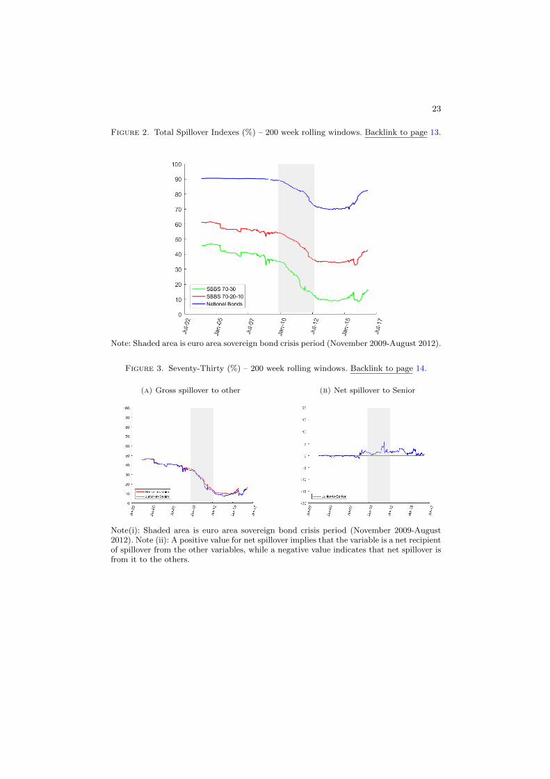
The TSI values over time for the 70-30 and 70-20-10 asset combinations are
shown in Figure 2. As per the full-sample tables, the two-asset case records
lower TSI values than the three-asset case over all windows. The gap between
the two widens during the crisis period and remains greater in the post-crisis
period than before the crisis. The third series in Figure 2 represents the rolling
total spillover index value for a VAR where the eleven variables in it are the first-
differences of the spreads of the aforementioned member state ten-year bond
yields over the US ten-year bond yield. The average spillover values among the
11 national sovereign bond markets are much higher in each estimation window
than when the yields from the 70-20 and 70-20-10 tranches are used.

14
Figure 3 shows the gross and net spillovers for the 70-30 tranche structure. As
with the entries for this pairing in Table 1, the gross spillovers to the senior
and junior securities in panel (A) are broadly in line with one another over
time. Both decline substantially during the crisis period from values of just
under 40% at its start to close to 10% by its end. An economic interpretation
of this development is that financial market stress leads to the senior and junior
securities being seen by investors as more distinct from one another. The gross
spillover values move in a narrow, low-value range after the crisis. Panel (B) of
Figure 3 indicates low net spillover values (usually no more than 3% in value)
between the senior and junior tranches in the 70-30 structure. Net spillover is
usually from the junior to the senior security.
Figure 4 covers the three-asset, 70-20-10 structure. The gross-spillover-from-
others values are shown in the panels on the left-hand-side of that figure. In
all three charts, the total gross spillover values have a downward trend over
time. This decline is strongest for the senior tranche (panel (A)). The other
two lines in that panel represent the spillover to the senior from the mezzanine
and from the junior tranches, as indicated in the panel’s labelling. There is a
larger spillover to the senior security from the mezzanine security than from
the junior security.
The declines in the total gross-spillover-from-others values over time are not as
strong in panels (C) and (E) of Figure 4, with most of those declines occurring
during the crisis period (as also occurs in panel (A)). There are differences in
how the components of these lines behave. In panel (C), the spillover from the
15
senior to the mezzanine security declines over time but that from the junior to
the mezzanine security rises. In a similar vein, the senior security’s spillover to
the junior security decreases (panel (E)) while that from the mezzanine to the
junior security increases. Looking across all three panels on the left-hand-side of
Figure 4, the gross spillovers to and from the senior security fall over time. The
bi-directional interaction between the mezzanine and the junior securities, as
measured by gross spillover values, is the largest amongst the variables during
the latter part of the crisis and after it. These developments can be interpreted
as the senior security becoming relatively detached from the other two securities
during the crisis and remaining so in its wake.
The net spillover values, shown in the panels on the right-hand-side column
of Figure 4, however, indicate the senior security, in general, being the largest
net recipient of spillover among the three, while the mezzanine security is the
largest net transmitter. The net spillover values for the junior tranche move
in a relatively narrow range around the origin over time. Among the three
assets, the mezzanine market then has the strongest net influence on the other
two.
4. Conclusion
Sovereign bond-backed securities (SBBS) have recently been espoused as
financial market instruments that could address safe asset shortages and
excessive bank-sovereign linkages in the euro area. The arguments for such

16
a securitisation and the form it could take have been outlined in Brunnermeier
et al. (2017). Their assessments of how effective the proposal would be in
generating safe assets merely address how the securitisation would insulate
senior bond holders from actual default-related losses. This paper generalises
the assessment by examining how the spillover of shocks within secondary
markets would be attenuated (i.e. how the spillovers among investment returns
on holdings of bonds/SBBS assets would be affected). Such an analysis is only
valid if plausible estimates of SBBS yields are available. We argue that the
approach of Schonbucher (2003) adequately addresses this need.
Given the aims of the SBBS proposal, the analysis presented here is reassuring.
The findings indicate that, in addition to the attenuation of default risk
exposures, the endogenous risks arising from secondary market spillovers would
be reduced under SBBS issuance. The spillover analysis applied to the senior-
junior yield series of the 70-30 structure and the senior-mezzanine-equity yields
of the 70-20-10 structure provides econometric output with a number of distinct
features. First, the tranching of sovereign bonds reduces spillover between
markets compared to a case where no tranching occurs. Secondly, comparing the
70-30 and 70-20-10 structures to one another reveals that average gross spillover
and net spillover values between markets are lower in the former case. Thirdly,
when a 70-20-10 structure is in place, the senior security market becomes
relatively more insulated from shocks in the two subordinated securities during
a period of financial stress.

17
The main caveat is that the historical bond data from which the SBBS yields are
derived can only be regarded as indicative of what would happen under similar
levels of stress in the future. How investors and securitisers would react in a
crisis when SBBS assets exist is not known and this could introduce risks that
are not part of the historical data upon which SBBS yields have been estimated.
Likewise, as argued by Brunnermeier et al. (2017), it may be that stress events
would be significantly less frequent and less severe in a scenario of actual SBBS
issuance. It is also possible that this analysis based on historical data (when
SBBS were absent) does not adequately reflect the beneficial effects that would
flow from SBBS investors being better able to match their risk preferences with
their ex ante risk exposures.
Being aware in advance of how losses would be allocated in the case of a
downturn, or period of stress, in bond markets is valuable to investors. Knowing
that the senior bond of the securitisation is protected from most losses -
regardless of where shocks are located - affords the investor the opportunity
to avoid such exposures at the outset. For investors willing to take higher risk
there is an opportunity to gain estimable exposures for an observable yield
premium when investing in the junior (and/or mezzanine) SBBS.
The challenges that remain are therefore mainly associated with the absence
of a true counterfactual for the behaviour of both individual sovereign bond
yield and yields on SBBS tranches. For example, with a larger supply of safe
assets (the senior SBBS) there is less likely to be a strong flight-to-safety effect
remaining in individual sovereign bond yield dynamics. Future research could

18
try to take these types of counterfactual realities into account when estimating
SBBS yields from historical data. This could be done by giving relatively more
weight to safer sovereigns in the SBBS estimation. This line of inquiry and other
extensions to address how actual defaults may interact with SBBS restructuring
and affect spillovers remain worthwhile avenues for future work.

19
References
Ang, A. and F. A. Longstaff (2013). Systemic sovereign credit risk: Lessons
from the U.S. and Europe. Journal of Monetary Economics 60 (5), 493–510.
Brunnermeier, M. K., L. Garicano, P. Lane, M. Pagano, R. Reis, T. Santos,
D. Thesmar, S. Van Nieuwerburgh, and D. Vayanos (2016, May). The
sovereign-bank diabolic loop and ESBies. American Economic Review Papers
and Proceedings 106 (5), 508–512.
Brunnermeier, M. K., S. Langfield, M. Pagano, R. Reis, S. van Nieuwerburgh,
and D. Vayanos (2017). ESBies: Safety in the tranches. Economic
Policy 32 (90), 175–219.
Conefrey, T. and D. Cronin (2015). Spillover in euro area sovereign bond
markets. The Economic and Social Review 46 (2), 197–231.
Danielsson, J. and H. S. Shin (2003). Endogenous Risk. in, “Modern Risk
Management: A History,” edited by Peter Field, 297–314. London: Risk
Books.
Danielsson, J., H. S. Shin, and J. Zigrand (2012). Endogenous and Systemic
Risk, chapter 2 in “Quantifying Systemic Risk” by Joseph G. Haubrich and
Andrew W. Lo, editors, University of Chicago Press.
De Grauwe, P. and Y. Ji (2013). Self fulfilling crises in the Eurozone: An
empirical test. Journal of International Money & Finance 34, 15–36.
20
Diebold, F. and K. Yilmaz (2012). Better to give than to receive: Predictive
directional measurement of volatility spillovers. International Journal of
Forecasting 28 (1), 57–66.
ESRB High-Level Task Force on Safe Assets (2018). Sovereign bond-backed
securities: A feasibility study. European Systemic Risk Board.
Koop, G., M. Pesaran, and S. Potter (1996). Impulse response analysis in
non-linear multivariate models. Journal of Econometrics 74 (1), 119–147.
Lucas, A., B. Schwaab, and X. Zhang (2017). Modelling financial sector tail
risk in the euro area. Journal of Applied Econometrics 32, 171–191.
Schonbucher, P. J. (2003). Credit Derivatives Pricing Models: Models, Pricing
and Implementation. London: Wiley.

21
Table 1. Seventy-Thirty tranche: full sample spillovers (%) (10 January2000 to 31 October 2016)Backlink to page 11, 12.
Senior Junior From others Net from othersSenior 83.9 16.1 16.1 0.4Junior 15.7 84.3 15.7 -0.4Contribution to others 15.7 16.1 31.8Contribution including own 100 100
TSI = 15.9
Note: A positive value for net spillover implies that the variable is a net recipient ofspillover from the other variable, while a negative value indicates that net spilloveris from that variable to the other.
Table 2. Seventy-Twenty-Ten tranche: full sample spillovers (%) (10 January 2000to 31 October 2016)Backlink to page 11, 12.
Senior Mezzanine Junior From others Net from othersSenior 70.2 24.5 5.3 29.8 8Mezzanine 17.6 51.1 31.2 48.8 -12Junior 4.2 36.3 59.5 40.5 4Contribution to others 21.8 60.8 36.5 119.1Contribution including own 92 111.9 96
TSI = 39.7
Note: A positive value for net spillover implies that the variable is a net recipient of spilloverfrom the other variables, while a negative value indicates that net spillover is from it to theothers.

22
Figure 1. Estimated Yields on SBBS Tranches & Selected Sovereigns (%).Backlink to page 8.
(a) 70:30 SBBS Yields
(b) 70:20:10 SBBS Yields
(c) Yields of DE, IT, GR & PT
Note: Shaded area is euro area sovereign bond crisis period (November 2009-August 2012).
23
Figure 2. Total Spillover Indexes (%) – 200 week rolling windows. Backlink to page 13.
Note: Shaded area is euro area sovereign bond crisis period (November 2009-August 2012).
Figure 3. Seventy-Thirty (%) – 200 week rolling windows. Backlink to page 14.
(a) Gross spillover to other (b) Net spillover to Senior
Note(i): Shaded area is euro area sovereign bond crisis period (November 2009-August2012). Note (ii): A positive value for net spillover implies that the variable is a net recipientof spillover from the other variables, while a negative value indicates that net spillover isfrom it to the others.

24
Figure 4. Seventy-Twenty-Ten (%) – 200 week rolling windows . Backlink to page 14,15.
(a) Gross spillover to Senior (b) Net spillover to Senior
(c) Gross spillover to Mezzanine (d) Net spillover to Mezzanine
(e) Gross spillover to Junior (f) Net spillover to Junior
Note(i): Shaded area is euro area sovereign bond crisis period (November 2009-August2012). Note (ii): A positive value for net spillover implies that the variable is a net recipientof spillover from the other variables, while a negative value indicates that net spillover isfrom it to the others.

We are grateful to Sam Langfield, Marco Pagano, Richard Portes, Philip Lane, Javier Suárez and members of the ESRB High-Level Task Force on Safe Assets for helpful comments.
David Cronin Central Bank of Ireland, Dublin, Ireland; email: [email protected]
Peter G. Dunne Central Bank of Ireland, Dublin, Ireland; email: [email protected]
Imprint and acknowledgements
© European Systemic Risk Board, 2018
Postal address 60640 Frankfurt am Main, Germany Telephone +49 69 1344 0 Website www.esrb.europa.eu
All rights reserved. Reproduction for educational and non-commercial purposes is permitted provided that the source is acknowledged.
Note: The views expressed in ESRB Working Papers are those of the authors and do not necessarily reflect the official stance of the ESRB, its member institutions, or the institutions to which the authors are affiliated.
ISSN 2467-0677 (pdf) ISBN 978-92-9472-018-4 (pdf) DOI 10.2849/6565 (pdf) EU catalogue No DT-AD-18-004-EN-N (pdf)


