downside risk optimization vs mean-variance optimization - bwg
TRANSCRIPT

Downside Risk Optimization vs Mean-VarianceOptimization
Andrea Rigamonti
Free University of Bozen-Bolzano
November 22, 2019

Introduction
Classical framework in modern portfolio theory:
• Investors care about mean and variance of the returns.
• Investors want to maximize the Sharpe ratio:
SR =R−Rf
σ. (1)
Most likely, real investors:
• Only consider downside deviation (variability below acertain benchmark) as risk.
• Care about mean and semivariance of the returns.
• Want to maximize the Sortino Ratio.

Introduction
Why is mean-variance optimization more popular?
• Mean-semivariance optimization requires the estimation ofa semicovariance matrix.
• “Traditional” obstacle: this matrix is endogenous.
• Additional issue: more parameter uncertainty.
• Other measures of downside risk, like CVaR, also performpoorly for the same reason.
Message of the paper: even if using downside risk is feasible,optimizing mean-variance remains preferable in most cases.

Background - Downside volatility
Minimizing variance is equivalent to minimizing downsidevolatility only if the return distribution is symmetric:
Symmetric distribution; risk = returns below mean
mean
downside volatility upside volatility
Skewed distribution; risk = returns below benchmark
mean benchmark
downside volatility upside volatility
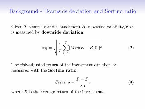
Background - Downside deviation and Sortino ratio
Given T returns r and a benchmark B, downside volatility/riskis measured by downside deviation:
σB =
√√√√ 1
T
T∑t=1
[Min(rt −B, 0)]2. (2)
The risk-adjusted return of the investment can then bemeasured with the Sortino ratio:
Sortino =R−BσB
, (3)
where R is the average return of the investment.
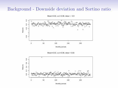
Background - Downside deviation and Sortino ratio
0 50 100 150 200
−0.
6−
0.2
0.0
0.2
Mean=0.02, s.d.=0.08, skew ≈ −3.9
Monthly periods
Ret
urns
0 50 100 150 200
0.0
0.2
0.4
0.6
0.8
Mean=0.02, s.d.=0.08, skew ≈ 5.83
Monthly periods
Ret
urns

Background - Downside deviation and Sortino ratio
The two series have exactly the same Sharpe Ratio.
With B = 0.005: for the negatively skewed one Sortino ratio =0.242; for the positively skewed one Sortino ratio = 0.491.
0 50 100 150 200 250
020
4060
80
Evolution of wealth (1 unit invested at period 0)
Monthly periods
Wea
lth
negative skew
positive skew
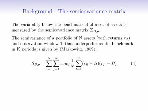
Background - The semicovariance matrix
The variability below the benchmark B of a set of assets ismeasured by the semicovariance matrix ΣB,p.
The semivariance of a portfolio of N assets (with returns rit)and observation window T that underperforms the benchmarkin K periods is given by (Markowitz, 1959):
SB,p =
N∑i=1
N∑j=1
wiwj1
N
K∑t=1
(rit −B)(rjt −B) (4)
Problem: using (4) to select the periods that underperform Byields an endogenous matrix. A change in the weights wi andwj changes K and therefore the elements of ΣB,p.
Optimization problems that use ΣB,p are intractable.

Background - Exogenous approximation of ΣB,p
Estrada (2008) solution: compute the elements of thesemicovariance matrix as:
ΣB,ij =1
T
T∑t=1
[Min(rit −B, 0) ·Min(rjt −B, 0)] (5)
• Equation (5) is based on whether individual assets (not theportfolio) underperform B → ΣB,ij is exogenous.
• ΣB,ij well approximates ΣB,p (and is symmetric).
Mean-semivariance optimization is now feasible!

How good is Estrada’s approximation?Cheremushkin (2009): approximation error is substantial unlessassets are positively correlated.
I compare the exact (numerical) and Estrada solution.
DownDev SortinoCorr. Skew Estrada Num. Estrada Num.
-0.013(-0.3,-0.3) 0.0371 0.0363 0.1894 0.2114(0.3,0.3) 0.0280 0.0268 0.2499 0.2932
0.003(-0.3,-0.3) 0.0323 0.0311 0.2779 0.2837(0.3,0.3) 0.0265 0.0245 0.3202 0.3371
0.300(-0.3,-0.3) 0.0328 0.0326 0.3391 0.3560(0.3,0.3) 0.0263 0.0261 0.4221 0.4467
0.743(-0.3,-0.3) 0.0566 0.0563 0.1388 0.1433(0.3,0.3) 0.0508 0.0506 0.1445 0.1481
Table 1: Downside deviation (min var/semivar portfolio) and Sortinoratio (mean-var/semivar portfolio) with skew normal returns and 240months rolling windows

Which strategy works better?
In-sample:
• Zero skew: optimizing mean-semivariance or mean-varianceis equivalent.
• Non-zero skew: each strategy is more efficient in terms ofits objective function.
But what happens out-of-sample?
• Equation (5) only uses a subset of the T observations.More parameter uncertainty in the semicovariancematrix.
• Zero skew: using variance is always preferable.
• Non-zero skew: using variance can still be superior even interms of downside risk/Sortino ratio.
Using the wrong objective function can be rational!

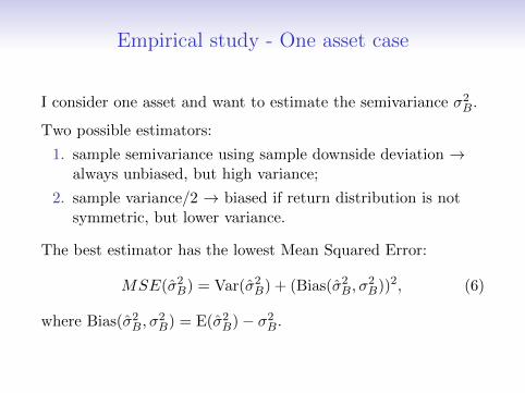
Empirical study - One asset case
I consider one asset and want to estimate the semivariance σ2B.
Two possible estimators:
1. sample semivariance using sample downside deviation →always unbiased, but high variance;
2. sample variance/2 → biased if return distribution is notsymmetric, but lower variance.
The best estimator has the lowest Mean Squared Error:
MSE(σ̂2B) = Var(σ̂2B) + (Bias(σ̂2B, σ2B))2, (6)
where Bias(σ̂2B, σ2B) = E(σ̂2B)− σ2B.
Empirical study - One asset case
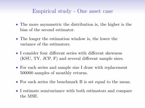
• The more asymmetric the distribution is, the higher is thebias of the second estimator.
• The longer the estimation window is, the lower thevariance of the estimators.
• I consider four different series with different skewness(KSU, TY, JCP, F) and several different sample sizes.
• For each series and sample size I draw with replacement500000 samples of monthly returns.
• For each series the benchmark B is set equal to the mean.
• I estimate semivariance with both estimators and comparethe MSE.

Empirical study - One asset case
200 400 600 800 1000 1200
5.0
e−
07
1.5
e−
06
Estimation window length
MS
E
TS: KSU; Skew = 0.0004; Kurt = 4.49
200 400 600 800 1000 1200
5.0
e−
08
1.0
e−
07
1.5
e−
07
Estimation window length
MS
E
TS: TY; Skew = −0.44; Kurt = 4.52
200 400 600 800 1000 1200
2.0
e−
07
6.0
e−
07
1.0
e−
06
1.4
e−
06
Estimation window length
MS
E
TS: JCP; Skew = 0.42; Kurtosis = 5.28
200 400 600 800 1000 12000.0
e+
00
4.0
e−
06
8.0
e−
06
1.2
e−
05
Estimation window length
MS
E
TS: F; Skew = 2.79; Kurtosis = 34.33
Sample semivariance Sample variance/2

Empirical study - Portfolio with two risky assets
Analogously to the case with one asset:
• For a given T, mean-semivariance should work better thanmean-variance if returns are sufficiently skewed.
• Given a non-zero skew, mean-semivariance should workbetter than mean-variance with a sufficiently high T.
Advantage of mean-variance: shrinkage estimators for thecovariance matrix (Ledoit & Wolf, 2004).
Does mean-semivariance optimization ever work well in realisticconditions?

Empirical study - Portfolio with two risky assets
• I consider four portfolios with two risky assets and oneriskless asset (risk-free rate from Fama-French).
• The pairs of assets have different degrees of skewness.
• I generate 500000 returns for each asset by drawing withreplacement from real empirical monthly returns series.
• I set the benchmark equal to the risk-free rate.
• Using the sample and shrunk covariance matrix, and theEstrada (2008) and numerical solution, I compute first theminimum variance/semivariance portfolios, and then themean-variance/semivariance portfolios.
• I use different rolling windows, and compare the downsidedeviation and Sortino ratio.

Minimum variance/semivariance portfolios
100 200 300 400 500 600 700 800
0.0
41
20
.04
16
0.0
42
00
.04
24
Estimation window length
Dow
nsid
e d
evia
tion
TS: KSU,GE; Skew = (0.0004,0.0006); Kurt = (4.49,4.25)
100 200 300 400 500 600 700 800
0.0
30
20
.03
06
0.0
31
00
.03
14
Estimation window length
Dow
nsid
e d
evia
tion
TS: EIX, TY; Skew = (−0.70,−0.44); Kurt = (7.69,4.52)
100 200 300 400 500 600 700 800
0.0
56
00
.05
64
0.0
56
8
Estimation window length
Dow
nsid
e d
evia
tion
TS: JCP, AJRD; Skew = (0.42,0.70); Kurt = (5.28,6.70)
100 200 300 400 500 600 700 800
0.0
46
50
.04
75
0.0
48
5
Estimation window length
Dow
nsid
e d
evia
tion
TS: ASH, F; Skew = (2.68,2.79); Kurt = (33.87,34.33)
Sample covariance Shrink covariance Semicovariance Num. semivariance
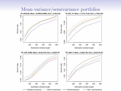
Mean-variance/semivariance portfolios
200 300 400 500 600
0.3
80
.42
0.4
60
.50
Estimation window length
Sort
ino r
atio
TS: KSU,GE; Skew = (0.0004,0.0006); Kurt = (4.49,4.25)
200 300 400 500 600
0.2
80
0.2
90
0.3
00
Estimation window length
Sort
ino r
atio
TS: EIX, TY; Skew = (−0.70,−0.44); Kurt = (7.69,4.52)
200 300 400 500 600
0.1
55
0.1
65
0.1
75
0.1
85
Estimation window length
Sort
ino r
atio
TS: JCP, AJRD; Skew = (0.42,0.70); Kurt = (5.28,6.70)
200 300 400 500 600
0.2
20
.24
0.2
60
.28
Estimation window length
Sort
ino r
atio
TS: ASH, F; Skew = (2.68,2.79); Kurt = (33.87,34.33)
Sample covariance Shrink covariance Semicovariance Num. semivariance

Results from two assets case
• Estrada (2008) never consistently outperforms thevariance-based portfolios.
• Minimizing the semivariance numerically is onlycompetitive with a positive skew and low kurtosis.
• High kurtosis seems to hurt semivariance-basedoptimization more than variance-based optimization.
Results might be better when the distribution is positivelyskewed because more observations fall below the benchmark.
I check if this holds with skew normal distributed returns withthe same mean and covariance but different skew.

Negative vs. positive skew
100 200 300 400 500 600 700 800
0.0
47
40
.04
78
0.0
48
2
Estimation window length
Dow
nsid
e d
evia
tion
Skew = (−0.5,−0.5)
100 200 300 400 500 600 700 800
0.0
35
60
.03
60
0.0
36
4
Estimation window length
Dow
nsid
e d
evia
tion
Skew = (0.5,0.5)
200 300 400 500 600
0.2
00
.22
0.2
40
.26
0.2
8
Estimation window length
Sort
ino r
atio
Skew = (−0.5,−0.5)
200 300 400 500 600
0.2
60
.28
0.3
00
.32
0.3
40
.36
Estimation window length
Sort
ino r
atio
Skew = (0.5,0.5)
Sample covariance Shrink covariance Semicovariance Num. semivariance

Alternative approach: minimizing CVaR
CVaR is a more popular measure of downside risk.
Lim et al. (2011) find that it suffers from similar problems.
I test 1/N, minimum variance (using Ledoit & Wolf, 2004),minimum semivariance (using Estrada, 2008) and minimumCVaR (95% CI) portfolios on real data:
• dataset: weekly DowJones returns (Feb 1990 - Apr 2016)from Bruni (2016);
• 5 and 10 years rolling window estimation;
• 843 out-of-sample returns;
• with and without short-selling (Jagannathan, 2003).

Alternative approach: minimizing CVaR
Strategy Dw. Dev. Sortino CVaR
1/N 0.0172 0.0791 -0.0555Min Var 0.0140 0.0552 -0.0449
Min Var Long 0.0139 0.0713 -0.0454Min Semivar 0.0163 0.0014 -0.0521
Min Semivar Long 0.0144 0.0485 -0.0459Min CVaR 0.0168 0.0047 -0.0539
Min CVaR Long 0.0148 0.0388 -0.0484
Table 2: 5 years rolling window estimation

Alternative approach: minimizing CVaR
Strategy Dw. Dev. Sortino CVaR
1/N 0.0172 0.0791 -0.0555Min Var 0.0138 0.0689 -0.0454
Min Var Long 0.0141 0.0795 -0.0465Min Semivar 0.0150 0.0132 -0.0483
Min Semivar Long 0.0145 0.0537 -0.0478Min CVaR 0.0148 0.0078 -0.0467
Min CVaR Long 0.0143 0.0546 -0.0469
Table 3: 10 years rolling window estimation

Conclusions
• Precise estimates of the semicovariance matrix are verydifficult to obtain.
• In a simulation study, minimizing the semivariance neverconsistently yields a lower downside deviation or higherSortino ratio than portfolios that minimize the variance.
• The CVaR has similar estimation issues.
• Both minimum semivariance and minimum CVaRportfolios fail to beat the minimum variance portfolio in anempirical application.
• Problem is in the concept of downside risk, not inthe way we measure it.
• The popularity of variance as a measure of risk is rationaland empirically justified.

Thank You!