Finance and Economics Discussion SeriesDivisions of Research & Statistics and Monetary Affairs

Federal Reserve Board, Washington, D.C.

Downside Variance Risk Premium

Bruno Feunou, Mohammad R. Jahan-Parvar and Cedric Okou

2015-020

Please cite this paper as:Bruno Feunou, Mohammad R. Jahan-Parvar and Cedric Okou (2015). “Downside VarianceRisk Premium,” Finance and Economics Discussion Series 2015-020. Washington: Board ofGovernors of the Federal Reserve System, http://dx.doi.org/10.17016/FEDS.2015.020.

NOTE: Staff working papers in the Finance and Economics Discussion Series (FEDS) are preliminarymaterials circulated to stimulate discussion and critical comment. The analysis and conclusions set forthare those of the authors and do not indicate concurrence by other members of the research staff or theBoard of Governors. References in publications to the Finance and Economics Discussion Series (other thanacknowledgement) should be cleared with the author(s) to protect the tentative character of these papers.

Downside Variance Risk Premium

Bruno Feunou∗ Mohammad R. Jahan-Parvar† Cedric Okou‡§

Bank of Canada Federal Reserve Board UQAM

March 2015

Abstract

We propose a new decomposition of the variance risk premium in terms of upside and downsidevariance risk premia. The difference between upside and downside variance risk premia is ameasure of skewness risk premium. We establish that the downside variance risk premium is themain component of the variance risk premium, and that the skewness risk premium is a pricedfactor with significant prediction power for aggregate excess returns. Our empirical investigationhighlights the positive and significant link between the downside variance risk premium and theequity premium, as well as a positive and significant relation between the skewness risk premiumand the equity premium. Finally, we document the fact that the skewness risk premium fills thetime gap between one quarter ahead predictability, delivered by the variance risk premium as ashort term predictor of excess returns and traditional long term predictors such as price-dividendor price-earning ratios. Our results are supported by a simple equilibrium consumption-basedasset pricing model.

Keywords: Risk-neutral volatility, Realized volatility, Downside and upside variance risk premium, Skew-

ness risk premium

JEL Classification: G12

∗Bank of Canada, 234 Wellington St., Ottawa, Ontario, Canada K1A 0G9. Email: feun@bankofcanada.ca.†Corresponding Author: Federal Reserve Board, 20th Street and Constitution Avenue NW, Washington, DC

20551 United States. E-mail: Mohammad.Jahan-Parvar@frb.gov‡Ecole des Sciences de la Gestion, University of Quebec at Montreal, 315 Sainte-Catherine Street East, Montreal,

Quebec, Canada H2X 3X2. Email: okou.cedric@uqam.ca§We thank seminar participants at the Federal Reserve Board, Johns Hopkins Carey Business School, Midwest

Econometric Group Meeting 2013, Manchester Business School, CFE 2013, and SNDE 2014. We are grateful forconversations with Diego Amaya, Sirio Aramonte, Federico Bandi, Nicola Fusari, Hening Liu, Olga Kolokolova,Bruce Mizrach, Maren Hansen, Yang-Ho Park, and Alex Taylor. We thank James Pinnington for research assistance.We also thank Bryan Kelly and Seth Pruitt for sharing their cross-sectional book-to-market index data. The viewsexpressed in this paper are those of the authors. No responsibility for them should be attributed to the Bank ofCanada or the Federal Reserve Board. Remaining errors are ours.

1 Introduction

In contrast to the traditional efficient-market hypothesis prediction that market returns are unpre-

dictable, current asset pricing research accepts that equity market returns are largely predictable

over long horizons. A number of recent studies have additionally argued that the variance risk

premium – the difference between option-implied and realized variance – yields superior forecasts

for stock market returns over shorter, within-year horizons (typically one quarter ahead). Exam-

ples of these studies include, among others, Bollerslev, Tauchen, and Zhou (2009); Drechsler and

Yaron (2011); and Kelly and Jiang (2014). Bollerslev, Tauchen, and Zhou (2009) (henceforth, BTZ)

show that the variance risk premium explains a nontrivial fraction of the time-series variation in

aggregate stock market returns, and that high (low) variance risk premia predict high (low) future

returns.

Drawing on the intuition that investors like good uncertainty – as it increases the potential of

substantial gains – but dislike bad uncertainty – as it increases the likelihood of severe losses – we

propose a new decomposition of the variance risk premium (VRP), expressed in terms of upside

and downside variance risk premia (V RPU and V RPD).1 We show that this decomposition a)

identifies the main sources of return predictability uncovered by BTZ and b) characterizes the role

of the skewness risk premium (SRP) – measured through the difference between V RPU and V RPD

– in predicting aggregate stock market returns. We find that on average, and similar to results

in Kozhan, Neuberger, and Schneider (2014), over 80% of the VRP is compensation for bearing

changes in downside risk. In addition, we show that a) the V RPD explains the empirical regularities

reported by BTZ (including the hump-shaped R2 and slope parameter patterns), b) the V RPU ’s

contribution to the results reported by BTZ is at best marginal, and c) there is a contribution of

the SRP to the predictability of returns which takes effect beyond the one-quarter-ahead window

documented by BTZ.

1We define the down(up)side variance as the realized variance of the stock market returns for negative (positive)returns, respectively. The down(up)side variance risk premium is the difference between option-implied and realizeddown(up)side variance. Decomposing variance in this way is pioneered by Barndorff-Nielsen, Kinnebrock, and Shep-hard (2010), and successfully used in empirical studies by Feunou, Jahan-Parvar, and Tedongap (2013, 2014), amongothers. In addition, we define the difference between upside and downside variances as the relative upside variance.Feunou, Jahan-Parvar, and Tedongap (2014) show that relative upside variance is a measure of skewness. Basedon their work, we use the difference between option-implied and realized relative upside variances as a measure ofskewness risk premium.

1

We show that the prediction power of V RPD and SRP increases over the term structure of

equity returns. In addition, through extensive robustness testing, we show that this result is robust

to the inclusion of a wide variety of common pricing factors. This leads to the conclusion that the

in-sample predictability of aggregate returns by downside risk and skewness measures introduced

here is independent from other common pricing ratios such as the price-dividend ratio, price-earning

ratio, or default spread. Based on revealed the in-sample predictive power of these measures, we

conduct out-of-sample forecast ability comparisons, and show that in comparison with V RPD and

SRP, other common predictors do not have a superior forecast ability. Finally, we study the link

between changes in downside variance risk and skewness risk premia and events or news related to

policy uncertainty, comparable to Amengual and Xiu (2014).

Theoretically, we support our findings by a simple endowment equilibrium asset pricing model,

where the representative agent is endowed with Epstein and Zin (1989) preferences, and where the

consumption growth process is affected by distinct upside and downside shocks. Our model shares

some features with Bansal and Yaron (2004), Bollerslev, Tauchen, and Zhou (2009), Segal, Shalias-

tovich, and Yaron (2015), among others. We show that under common distributional assumptions

for shocks to the economy, we can derive the equity risk premium, upside and downside variance risk

premium, and skewness risk premium in closed form. Our findings support the empirical findings

presented in the paper.

Similar to Colacito, Ghysels, and Meng (2014), our study is not an alternative to jump-tail risk

concerns – as studied in Bollerslev and Todorov (2011a,b) – or rare disaster models,in Nakamura,

Steinsson, Barro, and Ursua (2013). Our framework addresses asymmetries that are observed in

“normal times”. However, our model is well-suited and capable of addressing regularities that

emerge from a rare disaster happening, such as the Great Recession of 2007-2009. Essentially, our

approach provides simple yet insightful economic intuitions supporting the joint directional and

volatility jump risk of Bandi and Reno (2014). We show that our methodology is intuitive, easy to

implement, and generates robust predictions that close the horizon gap between short term models

such as BTZ and long-horizon predictive models such as Fama and French (1988), Campbell and

Shiller (1988), Cochrane (1991), and Lettau and Ludvigson (2001).

Our study is comprised of two natural and linked components. First, we study the role of

2

the V RPD as the main driver of the within-year predictability results documented by BTZ. In

this effort, we highlight the inherent asymmetry in responses of market participants to negative

and positive market outcomes. To accomplish this goal, we draw on the vast existing literature

on realized and risk-neutral volatility measures and their properties, to construct nonparametric

measures of up and downside realized and risk-neutral semi-variances. We then proceed to show

empirically how the stylized facts documented in the VRP literature are driven almost entirely

by the contribution of V RPD – the difference between realized and risk-neutral semi-variances

extracted from high frequency data. As in Chang, Christoffersen, and Jacobs (2013), our approach

avoids the traditional trade-off problem with estimates of higher moments from historical returns

data needing long windows to increase precision but short windows to obtain conditional instead of

unconditional estimates. Second, we show that using the relative upside variance of Feunou, Jahan-

Parvar, and Tedongap (2013, 2014), a nonparametric measure of skewness, we can enhance the

predictive power of the variance risk premium to horizons beyond one quarter ahead.2 Additionally,

we find and document the predictive power of a priced factor – the SRP – that fills the gap between

the variance risk premium and common long-term equity returns predictors.

Thus, we need reliable measures for realized and risk-neutral variance and skewness. A sizable

portion of empirical finance and financial econometrics literature is devoted to measures of volatility.

Canonical papers focused on properties and construction of realized volatility are Andersen, Boller-

slev, Diebold, and Ebens (2001a); Andersen, Bollerslev, Diebold, and Labys (2003); and Andersen,

Bollerslev, Diebold, and Labys (2001b), among others. The construction of realized downside and

upside volatilities (also known as realized semi-variances) is addressed in Barndorff-Nielsen, Kin-

nebrock, and Shephard (2010). We follow the consensus in the literature about construction of these

measures. Similarly, based on pioneering studies such as Carr and Madan (1998, 1999, 2001) and

Bakshi, Kapadia, and Madan (2003), we have a clear view on how to construct risk-neutral mea-

sures of volatility. The construction of option-implied downside and upside volatilities is addressed

in Andersen, Bondarenko, and Gonzalez-Perez (2014). Again, we follow the existing literature in

this respect.

On the other hand, traditional measures of skewness have well-documented empirical problems.

2The relative upside variance is the difference between the upside and downside variances.

3

Kim and White (2004) demonstrate the limitations of estimating the traditional third moment.

Harvey and Siddique (1999, 2000) explore time variation in conditional skewness by imposing au-

toregressive structures. More recently, Feunou, Jahan-Parvar, and Tedongap (2013) and Ghysels,

Plazzi, and Valkanov (2011) use Pearson and Bowley’s skewness measures, respectively. They over-

come many problems associated with the centered third moment, such as the excessive sensitivity

to outliers documented in Kim and White (2004), by using alternative and more robust measures.

Neuberger (2012) and Feunou, Jahan-Parvar, and Tedongap (2014) study the properties of real-

ized measures of skewness used in Amaya, Christoffersen, Jacobs, and Vasquez (2013) and Chang,

Christoffersen, and Jacobs (2013) in predicting the cross-section of returns at weekly frequency.

Building on results presented in Feunou, Jahan-Parvar, and Tedongap (2014, 2013), we first con-

firm that skewness – measured as the difference between upside and downside variances – is a priced

factor. We then provide new evidences that the SRP – measured as the difference between the risk

neutral and historical expectations of skewness – is both priced and has superior predictive power.

Our study is also related to the recent macro-finance literature which emphasizes the importance

of higher-order risk attitudes such as prudence – a precautionary behavior which characterizes the

aversion towards downside risk – in the determination of equilibrium asset prices. Among those

studies, Eeckhoudt and Schlesinger (2008) investigate necessary and sufficient conditions for an

increase in savings induced by changes in higher-order risk attitudes while Dionne, Li, and Okou

(2014) restate a standard consumption-based capital asset pricing model (using the concept of

expectation dependence) to show that consumption second-degree expectation dependence risk – a

proxy for downside risk which accounts for nearly 80% of the equity premium – is a fundamental

source of the macroeconomic risk driving asset prices.

Based on the work of Amengual and Xiu (2014), we document the links that macroeconomic

announcements and events share with the SRP and V RPD. Following Ludvigson and Ng (2009)

and Feunou, Fontaine, Taamouti, and Tedongap (2014), we survey in a robustness study the

correlations between VRP components and 124 macroeconomic and financial indicators. We find

a much lower correlation of the said macroeconomic and financial indicators with V RPD, as well

as with the SRP; the correlation is greater with the VRP, as well as with the V RPU .

We show through careful robustness exercises that the prediction power of V RPD and SRP

4

are independent from other common pricing variables. Additionally, in order to address data-

mining concerns raised by Goyal and Welch (2008), we conduct out-of-sample forecasting exercises

to establish that our predictive variables perform at least as well as other common pricing variables

in forecasting excess returns.

The rest of the paper proceeds as follows. In Section 2 we present our decomposition of the

VRP and the method for construction of risk-neutral and realized semi-variances, as well as the

relative upside variance – which is our measure of skewness. Section 3 details the data used in this

study and the empirical construction of predictive variables used in our analysis. We present and

discuss our main empirical results in Section 4. Specifically, we intuitively describe the components

of variance risk and skewness risk premia, link them to macroeconomic factors, to policy news,

discuss their predictive ability, and explore their robustness in Sections 4.1, 4.2, 4.3, 4.4, and 4.5,

respectively. In Sections 4.6 and 4.7, we investigate the out-of-sample forecasting performance of

our measures. In Section 5, we present a simple equilibrium consumption-based asset pricing model

that supports our empirical results. Section 6 concludes.

2 Decomposition of the Variance Risk Premium

In what follows, we decompose equity price changes into positive and negative returns with respect

to a suitably chosen threshold. In this study, we set this threshold to zero, but it can assume

other values, given the questions to be answered. We sequentially build measures for upside and

downside variances, and for skewness. When taken to data, these measures are constructed non-

parametrically.

We posit that stock prices or equity market indices such as the S&P 500, S, are defined over the

physical probability space characterized by (Ω,P,F), where Ft∞t=0 ∈ F are progressive filters on

F . The risk neutral probability measure Q is related to the physical measure P through Girsanov’s

change of measure relation dQdP |FT = ZT , T < ∞. At time t, we denote total equity returns as

Ret = (St +Dt − St−1)/St−1 where Dt is the dividend paid out in period [t− 1, t]. In high enough

sampling frequencies, Dt is effectively equal to zero. Then, we denote the log of prices by st = lnSt,

log-returns by rt = st − st−1 and excess log-returns by ret = rt − rft , where rft is the risk-free rate

observed at time t−1. We obtain cumulative excess returns by summing one-period excess returns,

5

ret→t+k =∑k

j=0 ret+j , where k is our prediction/forecast horizon.

2.1 Construction of the variance risk premium

We build the variance risk premium following the steps in BTZ as the difference between option-

implied and realized variances. Alternatively, these two components could be viewed as variances

under risk-neutral and physical measures, respectively. In our approach, this construction requires

four distinct steps: building the upside and downside variances under the physical measure, and

then doing the same under the risk neutral measure.

For a given trading day t, following Andersen et al. (2003, 2001a), we construct the realized

variance of returns as RVt =∑nt

j=1 r2j,t, where r2

j,t is the jth intraday log-return and nt is the number

of intraday returns observed on that day. We add the squared overnight log-return (the difference

in log price between when the market opens at t and when it closes at t − 1), and we scale the

RVt series to ensure that the sample average realized variance equals the sample variance of daily

log-returns. For a give threshold κ, we decompose the realized variance into upside and downside

realized variances following Barndorff-Nielsen, Kinnebrock, and Shephard (2010):

RV Ut (κ) =

nt∑j=1

r2j,tI[rj,t>κ], (1)

RV Dt (κ) =

nt∑j=1

r2j,tI[rj,t≤κ]. (2)

We add the squared overnight “positive” log-return (exceeding the threshold κ) to the upside

realized variance RV Ut , and the squared overnight “negative” log-return (falling below the threshold

κ) to the downside realized variance RV Dt . Because the daily realized variance sums the upside

and the downside realized variances, we apply the same scale to the two components of the realized

variance. Specifically, we multiply both components by the ratio of the sample variance of daily

log-returns over the sample average of the (pre-scaled) realized variance.

For a given horizon h, we obtain the cumulative realized quantities by summing the one-day

realized quantities over the h periods:

6

RV Ut,h(κ) =

h∑j=1

RV Ut+j(κ),

RV Dt,h(κ) =

h∑j=1

RV Dt+j(κ),

RVt,h =h∑j=1

RVt+j(κ). (3)

By construction, the cumulative realized variance adds up the cumulative realized upside and

downside variances:

RVt,h ≡ RV Ut,h(κ) +RV D

t,h(κ). (4)

Next, we characterize the V RP of BTZ through premia accrued to bearing upside and downside

variance risks, following these steps:

V RPt,h = EQt [RVt,h]− EP

t [RVt,h],

=(EQt [RV U

t,h(κ)]− EPt [RV U

t,h(κ)])

+(EQt [RV D

t,h(κ)]− EPt [RV D

t,h(κ)]),

V RPt,h ≡ V RPUt,h(κ) + V RPDt,h(κ). (5)

Eq. (5) represents the decomposition of the VRP of BTZ into upside and downside variance risk

premia – V RPUt,h(κ) and V RPDt,h(κ), respectively – that lies at the heart of our analysis.

2.1.1 Construction of P-expectation

The goal here is to evaluate EPt [RV U

t,h(κ)] and EPt [RV D

t,h(κ)]. To this end, we consider three

specifications:

• Random Walk

EPt [RV

U/Dt,h (κ)] = RV

U/Dt−h,h(κ),

where U/D stands for “U or D”; this is the model used in BTZ.

7

• U/D-HAR

EPt [RV

U/Dt+1 (κ)] = ωU/D + β

U/Dd RV

U/Dt (κ) + βU/Dw RV

U/Dt,5 (κ) + βU/Dm RV

U/Dt,20 (κ).

• M-HAR

EPt [MRVt+1(κ)] = ω + βdMRVt(κ) + βwMRVt,5(κ) + βmMRVt,20(κ),

where MRVt,h(κ) ≡ (RV Ut,h(κ), RV D

t,h(κ))′.

Both U/D-HAR and M-HAR specifications mimic Corsi (2009)’s HAR-RV model. To get gen-

uine expected values for realized measures that are not contaminated by forward bias or use of

contemporaneous data, we perform an out-of-sample forecasting exercise to predict the three real-

ized variances, at different horizons, corresponding to 1, 2, 3, 6, 9, 12, 18 and 24 months ahead. In

our subsequent analysis, we find that these alternative specifications provide similar results. Hence,

for simplicity and to save space, we only report the results based on the random walk model.

2.1.2 Construction of Q-expectation

To build the risk-neutral expectation of RVt,h, we follow the methodology of Andersen and

Bondarenko (2007):

EQt [RV U

t,h(κ)] ≈ EQt

[ ∫ t+h

tσ2uI[ln(Fu|Ft)>κ]du

],

= EQt

[ ∫ t+h

tσ2uI[Fu>Ft exp(κ)]du

].

Thus,

EQt [RV U

t,h(κ)] ≈ 2

∫ ∞Ft exp(κ)

M0(S)

S2 dS, (6)

M0(S) = min(Pt(S), Ct(S)),

where, Pt(S), Ct(S), and S are prices of European put and call options (with maturity h), and

the strike price of the underlying asset, respectively. Ft is the price of a future contract at time t,

8

defined as Ft = St exp(rft h). Similarly for EQt [RV D

t,h(κ)], we get:

EQt [RV D

t,h(κ)] ≈ 2

∫ Ft exp(κ)

−∞

M0(S)

S2 dS. (7)

We simplify our notation by renaming EQt [RV U

t,h(κ)] and EQt [RV D

t,h(κ)] as

IV Ut,h = EQ

t [RV Ut,h(κ)], (8)

IV Dt,h = EQ

t [RV Dt,h(κ)]. (9)

We refer to IVU/Dt,h as the “risk-neutral semi-variance” or “implied semi-variance” of returns. These

quantities are conditioned on the threshold value κ, which we suppress to simplify notation. As

evident in this section, our measures of realized and implied volatility are model-free.

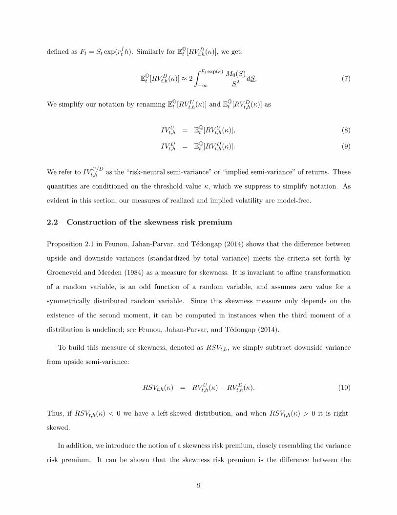
2.2 Construction of the skewness risk premium

Proposition 2.1 in Feunou, Jahan-Parvar, and Tedongap (2014) shows that the difference between

upside and downside variances (standardized by total variance) meets the criteria set forth by

Groeneveld and Meeden (1984) as a measure for skewness. It is invariant to affine transformation

of a random variable, is an odd function of a random variable, and assumes zero value for a

symmetrically distributed random variable. Since this skewness measure only depends on the

existence of the second moment, it can be computed in instances when the third moment of a

distribution is undefined; see Feunou, Jahan-Parvar, and Tedongap (2014).

To build this measure of skewness, denoted as RSVt,h, we simply subtract downside variance

from upside semi-variance:

RSVt,h(κ) = RV Ut,h(κ)−RV D

t,h(κ). (10)

Thus, if RSVt,h(κ) < 0 we have a left-skewed distribution, and when RSVt,h(κ) > 0 it is right-

skewed.

In addition, we introduce the notion of a skewness risk premium, closely resembling the variance

risk premium. It can be shown that the skewness risk premium is the difference between the

9

two components of the VRP and is defined as the difference between risk neutral and objective

expectations of the realized skewness. We denote skewness risk premium by SRPt,h, and construct

it as follows:

SRPt,h = EQ[RSVt,h]− EP[RSVt,h],

SRPt,h = V RPUt,h(κ)− V RPDt,h(κ). (11)

If RSVt,h < 0, we view SRPt,h as a skewness premium – the compensation for an agent who bears

downside risk. On the other hand, if RSVt,h > 0, we view SRPt,h as a skewness discount – the

amount that the agent is willing to pay to secure a positive return on an investment.

Since this measure of skewness risk premium is nonparametric and model-free, it is easier to

implement and interpret than competing parametric counterparts. Also, as mentioned earlier,

through a suitable choice of κ it can be used to investigate tail behavior of returns – if such an

exercise is desired. In this study, we are not interested in this application.

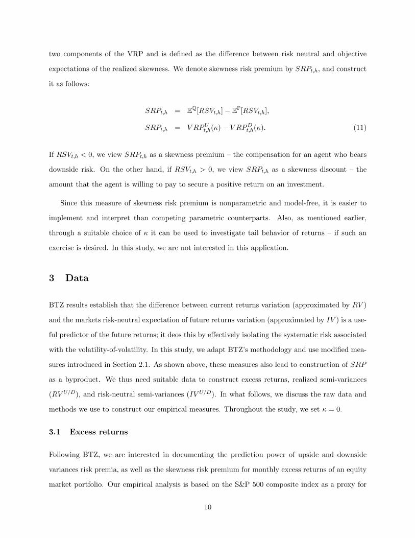
3 Data

BTZ results establish that the difference between current returns variation (approximated by RV )

and the markets risk-neutral expectation of future returns variation (approximated by IV ) is a use-

ful predictor of the future returns; it deos this by effectively isolating the systematic risk associated

with the volatility-of-volatility. In this study, we adapt BTZ’s methodology and use modified mea-

sures introduced in Section 2.1. As shown above, these measures also lead to construction of SRP

as a byproduct. We thus need suitable data to construct excess returns, realized semi-variances

(RV U/D), and risk-neutral semi-variances (IV U/D). In what follows, we discuss the raw data and

methods we use to construct our empirical measures. Throughout the study, we set κ = 0.

3.1 Excess returns

Following BTZ, we are interested in documenting the prediction power of upside and downside

variances risk premia, as well as the skewness risk premium for monthly excess returns of an equity

market portfolio. Our empirical analysis is based on the S&P 500 composite index as a proxy for

10

the aggregate market portfolio. Since our study requires reliable high-frequency data and option-

implied volatilities, our sample spans the September 1996 to December 2010 period. We construct

the excess returns by subtracting 3-month Treasury Bill rates from log-differences in the S&P 500

composite index, sampled at the end of each month.

We report the summary statistics of equity returns in Panel A of Table 1. We report annualized

mean, median, and standard deviations of returns in percentages. The table also reports monthly

skewness, excess kurtosis, and the first order autoregressive coefficient (AR(1)) for the S&P 500

monthly excess returns.

3.2 Options data and risk-neutral variances

Since our study hinges on decomposition of the variance process into upside and downside semi-

variances, we cannot follow BTZ by using VIX as a measure of risk-neutral volatility. As a result,

we construct our own measures of risk-neutral upside and downside variances (IV U/D). We use two

sources of data to construct upside and downside IV measures. First, we obtain from OptionMetrics

Ivy DB daily data of European-style put and call options on the S&P 500 index. We then match

these option data with return series on the underlying S&P 500 index and risk-free rates downloaded

from CRSP files.

For each day in the sample period, which begins in September 1996 and ends in December

2010, we sort call and put option data by maturity and strike price. We construct option prices by

averaging the bid and ask quotes for each contract. To obtain consistent risk-neutral moments, we

preprocess the data by applying the same filters as in Chang, Christoffersen, and Jacobs (2013).3 We

only consider out-of-the-money (OTM) contracts. Such contracts are the most traded, and thus, the

most liquid options. Thus, we discard call options with moneyness levels – the ratios of strike prices

to the underlying asset price – lower than 97% (S/S < 0.97). Similarly, we discard put options

with moneyness levels greater than 103% (S/S > 1.03). Raw option data contain discontinuous

strike prices. Therefore, on each day and for any given maturity, we interpolate implied volatilities

over a finely-discretized moneyness domain (S/S), using a cubic spline to obtain a dense set of

implied volatilities. We restrict the interpolation procedure to days that have at least two OTM

3That is, we discard options with zero bids, those with average quotes less than $3/8, and those whose quotesviolate common no-arbitrage restrictions.

11

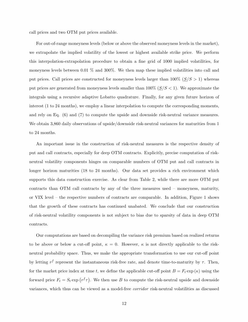
call prices and two OTM put prices available.

For out-of-range moneyness levels (below or above the observed moneyness levels in the market),

we extrapolate the implied volatility of the lowest or highest available strike price. We perform

this interpolation-extrapolation procedure to obtain a fine grid of 1000 implied volatilities, for

moneyness levels between 0.01 % and 300%. We then map these implied volatilities into call and

put prices. Call prices are constructed for moneyness levels larger than 100% (S/S > 1) whereas

put prices are generated from moneyness levels smaller than 100% (S/S < 1). We approximate the

integrals using a recursive adaptive Lobatto quadrature. Finally, for any given future horizon of

interest (1 to 24 months), we employ a linear interpolation to compute the corresponding moments,

and rely on Eq. (6) and (7) to compute the upside and downside risk-neutral variance measures.

We obtain 3,860 daily observations of upside/downside risk-neutral variances for maturities from 1

to 24 months.

An important issue in the construction of risk-neutral measures is the respective density of

put and call contracts, especially for deep OTM contracts. Explicitly, precise computation of risk-

neutral volatility components hinges on comparable numbers of OTM put and call contracts in

longer horizon maturities (18 to 24 months). Our data set provides a rich environment which

supports this data construction exercise. As clear from Table 2, while there are more OTM put

contracts than OTM call contracts by any of the three measures used – moneyness, maturity,

or VIX level – the respective numbers of contracts are comparable. In addition, Figure 1 shows

that the growth of these contracts has continued unabated. We conclude that our construction

of risk-neutral volatility components is not subject to bias due to sparsity of data in deep OTM

contracts.

Our computations are based on decompiling the variance risk premium based on realized returns

to be above or below a cut-off point, κ = 0. However, κ is not directly applicable to the risk-

neutral probability space. Thus, we make the appropriate transformation to use our cut-off point

by letting rf represent the instantaneous risk-free rate, and denote time-to-maturity by τ . Then,

for the market price index at time t, we define the applicable cut-off point B = Ft exp (κ) using the

forward price Ft = St exp(rfτ). We then use B to compute the risk-neutral upside and downside

variances, which thus can be viewed as a model-free corridor risk-neutral volatilities as discussed

12

in Andersen, Bondarenko, and Gonzalez-Perez (2014); Andersen and Bondarenko (2007) and Carr

and Madan (1999), among others.

Panel B of Table 1 reports the summary statistics of risk-neutral volatility measures. As ex-

pected, these series are persistent – AR(1) parameters are all above 0.95 – and demonstrate signif-

icant skewness and excess kurtosis. It is also clear that the main factor behind volatility behavior

is the downside variance.

Figure 2 provides a stark demonstration of this point. It is immediately obvious that the

contribution of upside variance to risk-neutral volatility is considerably less than that of downside

variance. In fact, for most maturities, the median upside variance is about 50 to 80% smaller

than the median downside variance. As time-to-maturity increases – a good measure for future

expectations – the size of the median IV U decreases. Notice that the size of this quantity is never

as large as the median IV D. On the other hand, the size of median IV D increases uniformly over

time-to-maturity, is close to median risk-neutral volatility values at each corresponding point in

time-to-maturity, and demonstrates the same pattern of median risk-neutral volatility.

Thus, compared to its upside counterpart, the downside risk-neutral variance is clearly the

main component of the risk-neutral volatility. We buttress this claim in the remainder of the paper

through empirical analysis.

3.3 High frequency data and realized variance components

We use daily close-to-close S&P 500 returns, realized variances data computed from 5-minute intra-

day S&P 500 prices and 3-Month Treasury Bill Rates for the period September 1996 to December

2010, which yields a total of 3,608 daily observations. The data is available through the Institute

of Financial Markets.

To construct the daily RV U/Ds series, we use intraday S&P 500 data. We sum the 5-minute

squared negative returns for the downside realized variance (RV D) and the 5-minute squared pos-

itive returns for the upside realized variance (RV U ). We nest add the daily squared overnight

negative returns to the downside semi-variance, and daily squared overnight positive returns to the

upside realized variance. The overnight returns are computed for 4:00 PM to 9:30 AM. The total

realized variance is obtained by adding the downside and the upside realized variance. For the

13

three series, we use a multiplicative scaling of the average total realized variance series to match

the unconditional variance of S&P 500 returns.4

4 Empirical Results

In this section, we provide economic intuition and empirical support for our proposed decomposition

of the variance risk premium. First, based on a sound financial rationale, we intuitively describe

the expected behavior of the components of variance risk premium and skewness risk premium.

We also present some empirical facts about the size and variability of these components. Since our

approach is non-parametric, these facts stand as challenges for realistic models (reduced-form and

general equilibrium). Second, we establish that decomposing the variance risk premium into upside

and downside variance risk premia reveals that while VRP components are positively correlated

with several macroeconomic and financial indicators, the level of spanning across these components

differ. Third, we study the reaction of variance risk premium components to macroeconomic and

financial announcements. In particular, we are interested in uncovering the relationship between

announcements that reduce or resolve uncertainty surrounding monetary or fiscal policy. Fourth,

we provide an extensive investigation of predictability of equity premia, based on variance premium

and its components as well as skewness risk premium. We empirically demonstrate the contribution

of downside risk and skewness risk premia and characterize the sources of VRP predictability doc-

umented by BTZ. Subsequently, we provide comprehensive robustness study. Finally, we conclude

with out-of-sample forecast ability properties of our proposed predictors – downside variance risk

and skewness risk premia.

4.1 Description of the variance risk premium components

The VRP can be interpreted as the premium a market participant is willing to pay to hedge against

variation in future realized volatilities. It is expected to be positive because of the intuition that

risk-averse investors dislike large swings in volatility, especially in “bad times”. This intuition is

rationalized within the general equilibrium model of BTZ, where it is shown that the variance risk

premium is in general positive and proportional to the volatility of volatility. We confirm these

4Hansen and Lunde (2006) discuss various approaches to adjusting open-to-close RV s.

14

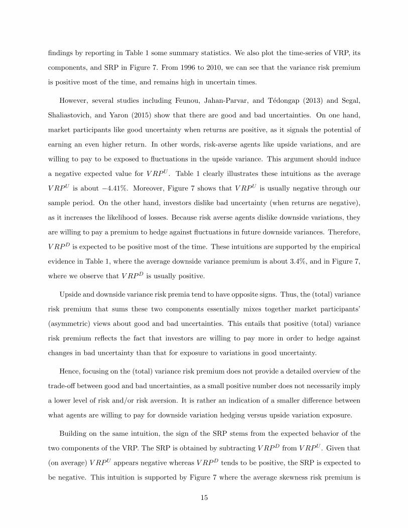
findings by reporting in Table 1 some summary statistics. We also plot the time-series of VRP, its

components, and SRP in Figure 7. From 1996 to 2010, we can see that the variance risk premium

is positive most of the time, and remains high in uncertain times.

However, several studies including Feunou, Jahan-Parvar, and Tedongap (2013) and Segal,

Shaliastovich, and Yaron (2015) show that there are good and bad uncertainties. On one hand,

market participants like good uncertainty when returns are positive, as it signals the potential of

earning an even higher return. In other words, risk-averse agents like upside variations, and are

willing to pay to be exposed to fluctuations in the upside variance. This argument should induce

a negative expected value for V RPU . Table 1 clearly illustrates these intuitions as the average

V RPU is about −4.41%. Moreover, Figure 7 shows that V RPU is usually negative through our

sample period. On the other hand, investors dislike bad uncertainty (when returns are negative),

as it increases the likelihood of losses. Because risk averse agents dislike downside variations, they

are willing to pay a premium to hedge against fluctuations in future downside variances. Therefore,

V RPD is expected to be positive most of the time. These intuitions are supported by the empirical

evidence in Table 1, where the average downside variance premium is about 3.4%, and in Figure 7,

where we observe that V RPD is usually positive.

Upside and downside variance risk premia tend to have opposite signs. Thus, the (total) variance

risk premium that sums these two components essentially mixes together market participants’

(asymmetric) views about good and bad uncertainties. This entails that positive (total) variance

risk premium reflects the fact that investors are willing to pay more in order to hedge against

changes in bad uncertainty than that for exposure to variations in good uncertainty.

Hence, focusing on the (total) variance risk premium does not provide a detailed overview of the

trade-off between good and bad uncertainties, as a small positive number does not necessarily imply

a lower level of risk and/or risk aversion. It is rather an indication of a smaller difference between

what agents are willing to pay for downside variation hedging versus upside variation exposure.

Building on the same intuition, the sign of the SRP stems from the expected behavior of the

two components of the VRP. The SRP is obtained by subtracting V RPD from V RPU . Given that

(on average) V RPU appears negative whereas V RPD tends to be positive, the SRP is expected to

be negative. This intuition is supported by Figure 7 where the average skewness risk premium is

15

−7.8%. Alternatively, this negative sign may be interpreted as follows: market participants prefer

higher skewness, and would like to be exposed to variations in future skewness.

Table 1 also reveals highly persistent, negatively-skewed, and fat-tailed distributions for (down/upside)

variance and skewness risk premia. Nonetheless, upside variance and skewness risk premia appear

more left-skewed and leptokurtic as compared to (total) variance and downside variance risk premia.

4.2 Links to macroeconomic and financial indicators

Following Ludvigson and Ng (2009) and Feunou et al. (2014), we survey the correlations of variance,

upside variance, downside variance, and skewness risk premia with 124 financial and economic

indicators. We carry out this exercise to document the contemporaneous correlation of variance

and skewness risk premia with well-known macroeconomic and financial variables. The VRP and its

components are predictors of risk in financial markets, that is, an increase in VRP or V RPD implies

expectations of elevated risk levels in the future and hence compensation for bearing that risk.

Fama and French (1989) document the counter-cyclical behavior of the equity premium: investors

demand a higher equity premium in bad times. It follows that VRP should be mildly pro-cyclical

and positively correlated with cyclical macroeconomic and financial variables. The relationship

between SRP and macroeconomic and financial factors is an empirically open issue that we address

in this study. Finally, we are interested in the spanning of VRP, its components, and SRP by

macroeconomic and financial factors. Briefly, low levels of spanning imply the information content

in the risk premium measures that is orthogonal to the information content of common financial

or economic quantities.

In our empirical investigation, we focus on contemporaneous correlations and adjusted R2s since,

given orthonormal factors, the regression coefficients depend on identification assumptions. The

analysis and results here are based on a contemporaneous univariate regression model, where the

dependent variable is one of the variance risk premium or skewness measures, and the independent

variable is one of the variables studied by Feunou et al. (2014).5

Table 3 reports the ten variables that yield the highest R2s for each (semi-)variance risk premium

component and their respective slope parameter Student-t statistics. The composition of the factors

5The complete list of these variables and supplementary results regarding our analysis are available in an onlineAppendix.

16

that explain the variation in variance, upside variance, downside variance, and skewness risk premia

and the size of the adjusted R2s above the 10% threshold wide-ranging. Clearly, variables listed

on this table all yield slope parameters statistically different from zero at conventional significance

levels, as evidenced by the high Student-t statistics.

Slope parameters for VRP and its components are all positive, and imply positive correlation

with the mainly pro-cyclical macroeconomic variables listed in the table. Overall, payroll measures

and industrial production indices are the most important predictors for VRP and its components,

accounting for virtually all top predictors for these quantities. Total payroll in the private sector

is the most powerful contemporaneous predictor for VRP and V RPU . It yields an adjusted R2 of

over 50% for V RPU and 40% for VRP. The level of explanatory power of this variable, measured

by the adjusted R2, drops to under 25% for V RPD.

Slope parameters for the regression model containing SRP as the predicted variable and macroe-

conomic and financial variables as predictors, imply a negative contemporaneous correlation. The

top variables with a significant correlation with SRP differ from those in the other three panels of

Table 3. For example, total payroll in the private sector does not have much explanatory power

for the SRP; it yields an adjusted R2 equal to 11.63% and is the 9th variable in the list. The

sources of predictability for the SRP – while much weaker – are diverse. Price indices and bond

yields have weak, contemporaneous prediction power for the SRP. Since payroll measures and bond

yields, especially those with shorter maturities such as 6-month Treasury Bills are pro-cyclical,

these findings imply counter-cyclical behavior for the SRP.

Together, the regularities discussed above lead us to conclude that the common financial and

macroeconomic indicators do not span well the VRP components or SRP, since none of them

explains more than 53% of the variation in these premia contemporaneously. Moreover, these

indicators seem to have the least success spanning downside variance and skewness risk premia.

This observation sheds further light on the success of these two factors in predicting equity premia

– their information content is largely uncorrelated with that of a large set of macroeconomic and

financial variables. Similarly, the relatively high correlation of V RPU with several macroeconomic

variables partially explains its poor predictive performance with respect to the equity premium –

it contains less unspanned information.

17

4.3 Reaction to announcements and events

Amengual and Xiu (2014) study the impact on decisions and announcements that reduce or resolve

uncertainty, especially regarding monetary and fiscal policies. We use the same set of events com-

piled by Amengual and Xiu (2014) to study the impact of events, such as FOMC announcements,

speeches by Federal Reserve officials and the Presidents of the United States, as well as economic

and political news that had significant impact on market returns or measures of market volatility.

The events are summarized in Table 4.

We report in Table 5 the changes in the variance, upside variance, downside variance, and

skewness risk premia as well as their end-of-the-day levels on event dates. The most striking outcome

from this exercise is the observation that across the board and for all variance risk components

and skewness risk premia, policy announcements that resolve financial or monetary uncertainty,

also reduce the premia. The impact on the SRP, however, is mixed: announcements can increase

or decrease the size of this premium. This observation, by construction, hinges on the size of the

reduction imputed by the announcement on V RPU and V RPD. That said, in 16 out of 22 events

studied, the impact of events on the SRP is negative.

In addition to matching the events recorded by Amengual and Xiu (2014) to changes in variance

risk premium components, we conducted an exercise to perform targeted searches for the largest

changes in variance risk premium components in suitably chosen date intervals that contain the

event date – in this case, a trading week before and after the event date – to identify the largest

changes in (semi-)variance risk premium components in that interval. The results are not funda-

mentally different from what is reported in Table 5. Most large movements are very close to the

event date. Thus they are not reported to save space, but are available upon request.

We may view these observations as evidence that resolution of policy uncertainty or reduction

of political tensions have a negative impact on premia demanded by the market participants to

bear variance or skewness risk.

4.4 Predictability of the equity premium

BTZ derive a theoretical model where the VRP emerges as the main driver of time variation in the

equity premium. They show both theoretically and empirically that a higher VRP predicts higher

18

future excess returns. Intuitively, the variance risk premium proxies the premium associated with

the volatility of volatility, which not only reflects how future random returns vary, but also assesses

fluctuations in the tail thickness of the future returns distribution.

Because the VRP sums downside and upside variance risk premia, BTZ’s framework entails

imposing the same coefficient on both (upside and downside) components of the VRP when they

are jointly included in a predictive regression of excess returns. However, such a constraint seems

very restrictive given the asymmetric views of investors on good uncertainty – proneness to upward

variability – versus bad uncertainty – aversion to downward variability. Sections 4.1, 4.2 and 4.3

document that both V RPD and V RPU have intrinsically different features.

Intuitively, risk-averse investors like variability in positive outcomes of returns, but dislike it

in negative outcomes. Hence in a joint regression, we expect coefficient of V RPD to be positive

and that of V RPU to be negative. These observations boil down to a simple intuition: risk-averse

investors ask for a premium to face risks they do not like while they are willing to pay for exposure

to favorable uncertainties – risks they like. Panel A in Table 9 reports results of joint regressions

of excess returns on both V RPD and V RPU . Our findings confirm our intuition at all horizons.

It is important to point out that by highlighting the disparities between upside and downside

variance risk premia, we do not intend to invalidate BTZ’s model. Their study is built to rationalize

the importance of variance risk premium in explaining the dynamics of the equity premium. Our

study pushes further, by documenting that the SRP is pivotal in disentangling the upside from the

downside premium related to future changes in variability. Thus, our goal is to build on BTZ’s

framework, showing that introducing asymmetry in the VRP analysis provides additional flexibility

to the trade-off between return first and second moment risk premia. Ultimately, our approach is

intended to strengthen the concept behind the variance risk premium of BTZ.

Our results are based on a simple linear regression of k-step-ahead cumulative S&P 500 excess

returns on values of a set of predictors that include the VRP, V RPU , V RPD, and SRP . Following

the results of Ang and Bekaert (2007), reported Student’s t-statistics are based on heteroscedasticity

and serial correlation consistent standard errors that explicitly take account of the overlap in the

regressions, as advocated by Hodrick (1992). The model used for our analysis is simply:

19

ret→t+k = β0 + β1xt(h) + εt→t+k, (12)

where rt→t+k is the cumulative excess returns between time t, t+ k, xt(h) is one of the predictors

discussed in Sections 2.1 and 2.2 at time t, h is the construction horizon of xt(h), and εt is a zero-

mean error term. We focus our discussion on the significance of the estimated slope coefficients

(β1s), determined by the robust Student-t statistics. We report the predictive ability of regressions,

measured by the corresponding adjusted R2s. For highly persistent predictor variables, the R2s for

the overlapping multi-period return regressions must be interpreted with caution, as noted by BTZ

and Jacquier and Okou (2014), among others.

Following our discussion of the observed mildly cyclical behavior of the VRP and those of

V RPU and V RPD in Section 4.2, and given the counter-cyclical behavior of the equity premium,

we expect to observe positive slope parameters in the regression model in equation (12), when xt(h)

is one of variance risk premia quantities.

We decompose the contribution of our predictors to show that: 1) predictability results doc-

umented by BTZ are driven by the downside variance risk premium, 2) predictability results are

mainly driven by risk-neutral expectations – thus, risk neutral measures contribute more than re-

alized measures, and 3) the contribution of the skewness risk premium increases as a function of

both the predictability horizon (k) and construction horizon (h).

Our empirical findings, presented in Tables 6 to 9, support all three claims made above. In Panel

A, Table 6, we show that the two main regularities uncovered by BTZ, hump-shaped increase in

robust Student-t statistics and adjusted R2s reaching their maximum at k = 3 (one quarter ahead),

are present in the data. Both regularities are visible in the upper-left-hand-side plots in Figures 4

and 5. These effects, however, weaken as the construction horizon (h) increases from one month to

three months or more: the predictability pattern weakens and then largely disappears for h > 6.

Panel B of Table 6 reports the predictability results based on using V RPD as the predictor.

A visual representation of these results is available in the upper-right-hand-side plots in Figures 4

and 5. It is immediately obvious that both regularities observed in the VRP predictive regressions

are preserved. We observe the hump-shaped pattern for Student’s t-statistics and the adjusted R2s

reaching their maximum between k = 3 or k = 6 months. Moreover, these results are more robust

20

to the construction horizon of the predictor. We notice that in contrast to the VRP results – where

predictability is only present for monthly or quarterly constructed risk premia – the V RPD results

are largely robust to construction horizons; the slope parameters are statistically different from

zero even for annually constructed downside variance risk premia (h = 12). Moreover, the V RPD

results yield higher adjusted R2s compared with the VRP regressions at similar prediction horizons,

an observation that we interpret as the superior ability of the V RPD to explain the variation in

aggregate excess returns. Last but not least, we notice a gradual shift in prediction results from

the familiar one-quarter-ahead peak of predictability documented by BTZ to 9-12-months-ahead

peaks, once we increase the construction horizon h. Based on these results, we infer that the the

V RPD is the likely candidate to explain the predictive power of VRP, documented by BTZ.

Our results for predictability based on the V RPU , reported in Panel C of Table 6 and the

two lower left-hand-side plots in Figures 4 and 5, are weak. The hump-shaped pattern in both

robust Student’s t-statistics and in adjusted R2s, while present, is significantly weaker than the

results reported by BTZ. Once we increase the construction horizon h, these results are lost. We

conclude that bearing upside variance risk does not appear to be an important contributor to the

equity premium, and hence, is not a good predictor of this quantity. In addition, we interpret these

findings as a low contribution of the V RPU to overall VRP.

We observe a set of interesting regularities, however, when we use the SRP as our predictor.

These results are reported in Panel D of Table 6 and the bottom-right-hand-side plots in Figures

4 and 5. It is immediately clear that this factor displays predictive power at longer horizons

than the VRP. For monthly excess returns, the SRP slope coefficient is statistically different from

zero at prediction horizons of 6-months-ahead or longer. At k = 6, the adjusted R2 of the SRP

is comparable in size with that of the VRP (2.30% against 3.65%, respectively) and is strictly

greater thereafter. At k = 6, the adjusted R2 for the monthly excess return regression based on

the SRP is smaller than that of the V RPD. However, their sizes are comparable at k = 9 and

k = 12 months ahead. Both trends strengthen as we consider higher aggregation levels for excess

returns. At the semi-annual construction level (h = 6), the SRP already has more predictive power

than both the VRP and V RPD at a quarter-ahead prediction horizon. The increase in adjusted

R2s of the SRP is not monotonic in the construction horizon level. We can detect a maximum

21

at a roughly three-quarters-ahead prediction window for semi-annual and annually constructed

SRPs. This observation implies that this factor is the intermediate link between one-quarter-ahead

predictability using the VRP uncovered by BTZ and the long-term predictors such as the price-

dividend ratio, dividend yield, or consumption-wealth ratio of Lettau and Ludvigson (2001). We

conclude that predictability of cumulative excess returns by the SRP increases in both prediction

horizon, k, and construction horizon, h, for the SRP.

At this point, it is natural to inquire about including both VRP components in a predictive

regression. We present the empirical evidence from this estimation in Panel A of Table 9. After

inclusion of the V RPU and V RPD in the same regression, the statistical significance of the V RPU ’s

slope parameters is broadly lost. We also notice a sign change in Student’s t-statistics associated

with the estimated slope parameters of the V RPU and V RPD. This observation, as documented in

Feunou, Jahan-Parvar, and Tedongap (2013), lends credibility to the role of the SRP as a predictor

of aggregated excess returns.6

We claim that the patterns discussed above, and hence the predictive power of the VRP, V RPD,

and SRP are rooted in expectations. That is, the driving force behind our results, as well as those

of BTZ, are expected risk-neutral measures of the volatility components. To show the empirical

findings supporting our claim, we run predictive regressions, using Equation (12). Instead of using

the “premia” employed so far, we use realized and risk-neutral measures of variances, up- and

downside variances, and skewness for xt, based on our discussions in Section 2, respectively.

Our empirical findings using risk-neutral volatility measures are available in Table 7. In Panel

A, we report the results of running a predictive regression when the predictor is the risk-neutral

variance obtained from direct application of the Andersen and Bondarenko (2007) method. It is

clear that the estimated slope parameters are statistically different from zero for k ≥ 3 at most

construction horizons, h. The reported adjusted R2s also imply that the predictive regressions have

explanatory power for aggregate excess return variations at k ≥ 3. The same patterns are discernible

for risk-neutral downside and upside variances (Panels B and C) and risk-neutral skewness (Panel

D). Adjusted R2s reported are lower than those reported in Table 6, and these measures of variation

6Briefly, based on arguments similar to those advanced by Feunou, Jahan-Parvar, and Tedongap (2013), we expectestimated parameters of the V RPU and V RPD to have opposite signs, and be statistically “close”. As such, theyimply that the SRP is the factor we should have included.

22

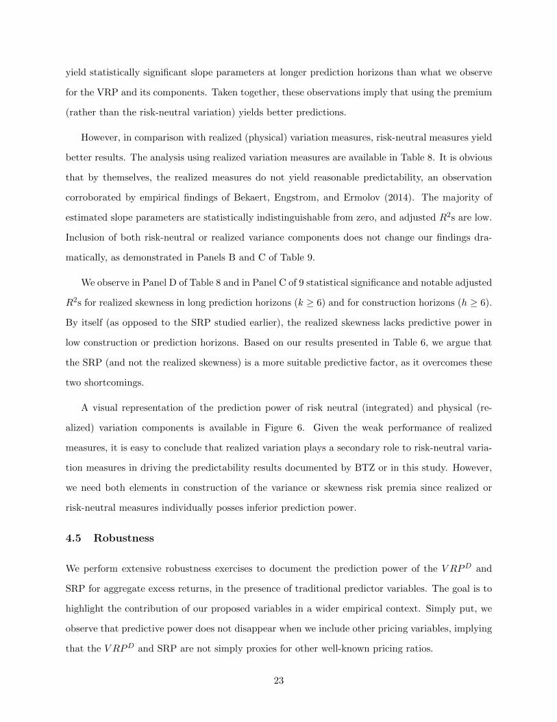
yield statistically significant slope parameters at longer prediction horizons than what we observe

for the VRP and its components. Taken together, these observations imply that using the premium

(rather than the risk-neutral variation) yields better predictions.

However, in comparison with realized (physical) variation measures, risk-neutral measures yield

better results. The analysis using realized variation measures are available in Table 8. It is obvious

that by themselves, the realized measures do not yield reasonable predictability, an observation

corroborated by empirical findings of Bekaert, Engstrom, and Ermolov (2014). The majority of

estimated slope parameters are statistically indistinguishable from zero, and adjusted R2s are low.

Inclusion of both risk-neutral or realized variance components does not change our findings dra-

matically, as demonstrated in Panels B and C of Table 9.

We observe in Panel D of Table 8 and in Panel C of 9 statistical significance and notable adjusted

R2s for realized skewness in long prediction horizons (k ≥ 6) and for construction horizons (h ≥ 6).

By itself (as opposed to the SRP studied earlier), the realized skewness lacks predictive power in

low construction or prediction horizons. Based on our results presented in Table 6, we argue that

the SRP (and not the realized skewness) is a more suitable predictive factor, as it overcomes these

two shortcomings.

A visual representation of the prediction power of risk neutral (integrated) and physical (re-

alized) variation components is available in Figure 6. Given the weak performance of realized

measures, it is easy to conclude that realized variation plays a secondary role to risk-neutral varia-

tion measures in driving the predictability results documented by BTZ or in this study. However,

we need both elements in construction of the variance or skewness risk premia since realized or

risk-neutral measures individually posses inferior prediction power.

4.5 Robustness

We perform extensive robustness exercises to document the prediction power of the V RPD and

SRP for aggregate excess returns, in the presence of traditional predictor variables. The goal is to

highlight the contribution of our proposed variables in a wider empirical context. Simply put, we

observe that predictive power does not disappear when we include other pricing variables, implying

that the V RPD and SRP are not simply proxies for other well-known pricing ratios.

23

Following BTZ and Feunou et al. (2014) among many others, we include equity pricing measures

such as log price-dividend ratio (log(pt/dt)), lagged log price-dividend ratio (log(pt−1/dt), and

log price-earning ratio (log(pt/et)); yield and spread measures such as term spread (tmst ) – the

difference between 10-year U.S. Treasury Bond yield and 3-month U.S. Treasury Bill yield –, default

spread (dfst) – the difference between BBB and AAA corporate bond yields –; CPI inflation (inflt),

and finally Kelly and Pruitt (2013) partial least squares-based, cross-sectional in-sample and out-

of-sample predictive factors (kpist and kpost, respectively).

We consider two periods for our analysis: our full sample – September 1996 to December 2010

– and a pre-Great Recession sample – September 1996 to December 2007. The latter ends at the

same point in time as the BTZ sample. We report our empirical findings in Tables 10 to 13. These

results are based on semi-annually aggregated excess returns and estimated for the one-month-

ahead prediction horizon.7 In this robustness study, we scale the cumulative excess returns; we use

ret→t+6/6 as the predicted value and regress it on a one-month lagged predictive variable.

Full-sample simple predictive regression results are available in Table 10. Among VRP com-

ponents, only the downside variance risk premium (dvrpt) and skewness risk premium (srpt) have

slope parameters that are statistically different from zero and have adjusted R2s comparable in

magnitude with other pricing variables. Once we use dvrpt along with other pricing variables, we

observe the following regularities in Table 11 which reports the following joint multi-variate regres-

sion results. First, the estimated slope parameter for dvrpt is statistically different from zero in all

cases, except when we include srpt. This result is not, however, surprising since srpt and dvrpt are

linearly dependent. Second, these regressions yield adjusted R2s which range between 3.10% (for

dvrpt and tmst, in line with findings of BTZ that report weak predictability for tmst) to 25.71%

(for dvrpt and inflt).8 The downside variance risk premium in conjuncture with the variance risk

premium or upside variance risk premium remains statistically significant and yields adjusted R2s

that are in the 7% neighborhood.

7A complete set of robustness checks, including monthly, quarterly, and annually aggregated excess returns results,are available in an online Appendix.

8The dynamics of inflation during the Great Recession period mimic the behavior of our variance risk premia.Gilchrist et al. (2014) meticulously study the behavior of this variable in the 2007-2009 period. According to theirstudy, both full and matched PPI inflation in their model display an aggregate drop in 2008-2009, while the reactionof financially sound and weak firms are asymmetric, with the former lowering prices and the latter raising prices inthis period. Thus, the predictive power of this variable, given the inherent asymmetric responses, is not surprising.

24

We obtain adjusted R2s that are decidedly lower than those reported by BTZ for quarterly and

annually aggregated multivariate regressions. These differences are driven by inclusion of the Great

Recession period data in our full sample. To illustrate this point, we repeat our estimation with

the data set ending in December 2007. Simple predictive regression results based on this data are

available in Table 12. We immediately observe that exclusion of the Great Recession period data

improves even the univariate predictive regression adjusted R2s across the board. The estimated

slope parameters are also closer to BTZ estimates and generally statistically significant.

In Table 13, we report multivariate regression results, based on 1996-2007 data. We notice that

once dvrpt is included in the regression model, the variance risk premium, upside variance risk

premium and skewness risk premium are no longer statistically significant. Other pricing variables,

except for term spread, default spread, and inflation, yield slope parameters that are statistically

significant. Thus, inflation seems to lack prediction power in this sub-sample. We do not observe

statistically insignificant slope parameters for the downside variance risk premium except when we

include vrpt. Across the board, adjusted R2s are high in this sub-sample.

4.6 Out-of-sample analysis

Our goal in this section is to compare the forecast ability of downside variance and skewness risk

premia with common financial and macroeconomic variables used in equity premium predictability

exercises.

To assess the ability of downside variance risk and skewness risk premia to forecast excess re-

turns, we follow the literature on predictive accuracy tests. We assume a benchmark model (B)

and a competitor model (C) in order to compare their predictive power for a given sample yTt=1.

To generate k-period out-of-sample predictions yt+k|t for yt+k, we split the total sample of T obser-

vations into in-sample and out-of-sample portions, where the first 1, . . . , tR in-sample observations

are used to obtain the initial set of regression estimates. The out-of-sample observations span the

last portion of the total sample t = tR + 1, . . . , T and are used for forecast evaluation. The models

are recursively estimated with the last in-sample observation ranging from t = tR to t = T − k,

at each t forecasting t + k. That is, we use time t data to forecast the k-step ahead value. In our

analysis, we use half of the total sample for the initial in-sample estimation, that is tR = bT2 c where

25

byc denotes the largest integer that is less than or equal to y. In order to generate subsequent sets

of forecasts, we employ a recursive scheme (expanding window), even though the in-sample period

can be fixed or rolling. The forecast errors from the two models are

eBt+k|t = yt+k − yBt+k|t,

eCt+k|t = yt+k − yCt+k|t,

where t = tR, . . . , T − k. Thus, we obtain two sets of t = T − tR − k + 1 recursive forecast errors.

The accuracy of each forecast is measured by a loss function L(•). Among the popular loss

functions are the squared error loss L(et+k|t) = (et+k|t)2 and the absolute error loss L(et+k|t) =

|et+k|t|. Let dBCt = L(et+k|t)B−L(et+k|t)

C be the error loss differential between the benchmark and

competitor models, and denote the expectation operator by E(•). To gauge if a model yields better

forecasts than an alternative specification, a two-sided test may be run, where the null hypothesis

is that the “two models have the same forecast accuracy” against the alternative hypothesis that

the “two models have different forecast accuracy”. Formally:

H0 : E(dBCt ) = 0 vs. HA : E(dBCt ) 6= 0.

Alternatively, a one-sided test may be considered, where the null hypothesis is that “model C does

not improve the forecast accuracy compared to model B” against the alternative hypothesis that

“model C improves the forecast accuracy compared to model B”. Formally:

H0 : E(dBCt ) ≤ 0 vs. HA : E(dBCt ) > 0.

In the context of our study, we apply forecast accuracy tests to non-nested models. The inno-

vation of our analysis is to introduce two new predictors, the V RPD and SRP. We compare the

benchmark model B, which includes our proposed predictors, and the competitor C, which con-

tains a traditional predictive variable such as the price-dividend ratio, dividend yield, price-earning

ratio, etc. Failure to reject the null leads us to conclude that the classical predictor does not yield

more accurate forecasts than our proposed predictor. Diebold and Mariano (1995) and West (1996)

26

provide further inference results on this class of forecast accuracy tests.

4.7 Out-of-sample empirical findings

Following the influential study of Inoue and Kilian (2004), we first investigate the in-sample fit of

the data by our proposed predictors – the V RPD and SRP – and traditional predictors studied in

the literature. Inoue and Kilian (2004) convincingly argue that to make dependable out-of-sample

inference, we need reasonable in-sample fit. The second column of Table 14 reports adjusted R2s

for monthly, quarterly, and semi-annually aggregated excess returns regressed on our proposed and

traditional predictors. These are in-sample results and no forecasting is performed. We notice

that, first, for all predictors, adjusted R2s improve with the prediction horizon. Second, we notice

that for all predictors except Kelly and Pruitt’s 2013 out-of-sample cross-sectional book-to-market

index, adjusted R2s are reasonably high. The Kelly-Pruitt index is by construction an out-of-sample

predictor. Thus, the seemingly poor in-sample performance is not a cause for concern for us.

Once we establish the in-sample prediction power, we move to investigate out-of-sample forecast

ability. Not surprisingly, out-of-sample adjusted R2s – reported in the third column of Table 14 –

are much smaller than their in-sample counterparts, with the exception of the Kelly-Pruitt index.

This observation may be due to inclusion of data from the 2007-2009 Great Recession period in the

out-of-sample exercise. As documented in Section 4.5, most predictors lose significant prediction

power once data from this period is included in the analysis.

Our task is to investigate the relative forecast performance of our proposed downside and

skewness risk premium measures against other well-known predictors. To this end, we implement

the Diebold and Mariano (1995) (henceforth, DM) tests of prediction accuracy. The results of

performing out-of-sample forecast accuracy tests are available in the fourth and the sixth column

of Table 14, where we report DM test statistics, and in the fifth and the seventh columns of the

same Table, where we report the associated p-values. We cannot reject the null of equal or superior

forecast accuracy when the benchmark is the downside variance (or skewness) risk premium and

the alternative model contains one of the traditional predictors, since p-values are greater than the

conventional 5% test size. We note the following important considerations. First, these results

are based on the DM forecast accuracy test for non-nested models. Our findings are robust for

27

all the horizons we consider in our analysis (1, 3 and 6 months). Second, the null hypothesis

states that the mean squared forecast error of the alternative model is larger than or equal to that

of the benchmark model. This is a one-sided test, and negative DM statistics indicate that the

alternative model performed worse than the benchmark model. Third, we interpret the p-values

cautiously, following Boyer, Jacquier, and van Norden (2012). They point out that p-values are

hard to interpret due to the Lindley-Smith paradox, and in addition, they need to be adjusted.

To be precise, we produce multiple p-values in this analysis. Using unadjusted p-values in such

an environment overstates the evidence against the null. Thus, following Boyer, Jacquier, and van

Norden (2012), we apply a Bonferroni adjustment to the generated p-values. Our reported findings

are, therefore, suitably conservative and reliable. Conventional competing variables such as the

variance risk premium, price-dividend ratio, and price-earning ratio, have lower forecast accuracy

than our proposed measures.

In a nutshell, the prediction power of the downside variance risk premium and skewness risk

premium are not a figment of good in-sample fit of the data. In comparison with other pricing

ratios and variables, our proposed measures have at least similar (and often superior) out-of-sample

accuracy.

5 A Simple Equilibrium Model

Our goal in this section is to show that our empirical findings are supported by a simple equilibrium

consumption-based asset pricing model. Our main objective is to highlight the roles that upside

and downside variance play in pricing a risky asset in an otherwise standard asset pricing model. In

particular, we show that under standard and mild assumptions, the weights and the signs attributed

to upside and downside variances are inline with our empirical findings. To save space, we only

report the main results. An online Appendix reports our derivations in great detail.

5.1 Preferences

We consider a endowment economy in discrete time. The representative agent’s preferences over

the future consumption stream are characterized by Kreps and Porteus (1978) intertemporal pref-

erences, as formulated by Epstein and Zin (1989) and Weil (1989):

28

Ut =

[(1− δ)C

1−γθ

t + δ(EtU1−γ

t+1

) 1θ

] θ1−γ

, (13)

where Ct is the consumption bundle at time t, δ is the subjective discount factor, γ is the coefficient

of risk aversion, and ψ is the elasticity of intertemporal substitution (IES). Parameter θ is defined

as θ ≡ 1−γ1− 1

ψ

. If θ = 1, then γ = 1/ψ and EZ preferences collapse to expected power utility, which

implies an agent who is indifferent to the timing of resolution of uncertainty of the consumption

path. With γ > 1/ψ, the agent prefers early resolution of uncertainty. For γ < 1/ψ, the agent

prefers late resolution of uncertainty. Epstein and Zin (1989) show that the logarithm of stochastic

discount factor (SDF) implied by these preferences is given by:

lnMt+1 = mt+1 = θ ln δ − θ

ψ∆ct+1 + (θ − 1)rc,t+1, (14)

where ∆ct+1 = ln(Ct+1

Ct

)is the log growth rate of aggregate consumption, and rc,t is the log return

of the asset that delivers aggregate consumption as dividends. This asset represents the returns on

a wealth portfolio. The Euler equation states that

Et [exp (mt+1 + ri,t+1)] = 1, (15)

where rc,t represents the log returns for the consumption generating asset (rc,t). The risk-free rate,

which represents the returns on an asset that delivers a unit of consumption in the next period

with certainty, is defined as:

rft = ln

[1

Et(Mt+1)

]. (16)

5.2 Consumption Dynamics under the Physical Measure

Our specification of consumption dynamics incorporates elements from Bansal and Yaron (2004),

Bekaert, Engstrom, and Ermolov (2014), and especially BTZ and Segal, Shaliastovich, and Yaron

(2015).

Fundamentally, we follow Bansal and Yaron (2004) in assuming that consumption growth has

a predictable component. We differ from Bansal and Yaron in assuming that the predictable

29

component is proportional to consumption growth’s upside and downside volatility components:9

∆ct+1 = µ0 + µ1Vu,t + µ2Vd,t + σc (εu,t+1 − εd,t+1) , (17)

where εu,t+1 and εd,t+1 are two mean-zero shocks that affect both the realized and expected con-

sumption growth.10 εu,t+1 represents upside shocks to consumption growth, and εd,t+1 stands for

downside shocks. Following Bekaert, Engstrom, and Ermolov (2014) and Segal, Shaliastovich, and

Yaron (2015), we assume that these shocks follow a demeaned Gamma distribution and model them

as

εi,t+1 = εi,t+1 − Vi,t i = u, d, (18)

where εi,t+1 ∼ Γ(Vi,t, 1). These distributional assumptions imply that volatilities of upside and

downside shocks are time-varying and driven by shape parameters Vu,t and Vd,t. In particular, we

have that

V art[εi,t+1] = Vi,t, i = u, d. (19)

Naturally, the total conditional variance of consumption growth when εu,t+1 and εd,t+1 are condi-

tionally independent, is simply σ2c (Vu,t + Vd,t).

As a result, sign and size of µ1 and µ2 matter in this context. With µ1 = µ2, we have a

stochastic volatility component in the conditional mean of consumption growth process, similar to

the classic GARCH-in-Mean structure for modeling risk-return trade-off in equity returns. With

both slope parameters equal to zero, the model yields the BTZ unpredictable consumption growth.11

If |µ1| = |µ2|, with µ1 > 0 and µ2 < 0, we have Skewness-in-Mean, similar in spirit to Feunou,

9Segal, Shaliastovich, and Yaron (2015) maintain this assumption in their definition of the long-run risk component.10This assumption is for the sake of brevity. Violating this assumption adds to algebraic complexity, but does not

affect our analytical findings.11It can be shown that assuming an unpredictable consumption growth process does not support the existence of

distinct upside and downside variance risk premia that are supported by empirical evidence, if we assume agentsendowed with Epstein and Zin (1989) preferences. In particular we have found that combining constant expectedconsumption growth with Epstein and Zin (1989) preferences will always yields positive upside variance risk-premium,which is in contradiction with our empirical findings. Using asymmetric preferences, such as smooth ambiguityaversion preferences of Klibanoff, Marinacci, and Mukerji (2009) or disappointment aversion of Gul (1991), it may bepossible to derive plausible upside and downside variance risk premia for an economy with unpredictable consumptiongrowth. The cost we pay is the loss of closed form analytical results. Miao, Wei, and Zhou (2012) use smooth ambiguityaversion preferences to motivate their study of variance risk premium, but assume time-variation in the conditionalmean of the consumption growth.

30

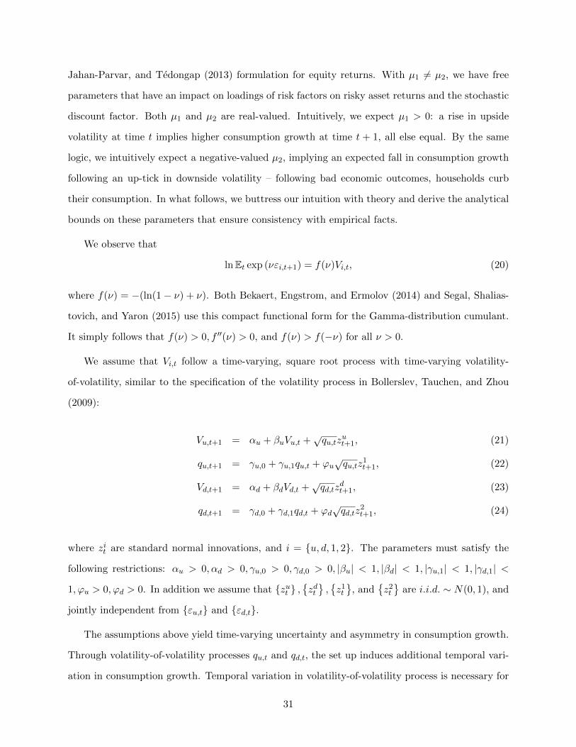
Jahan-Parvar, and Tedongap (2013) formulation for equity returns. With µ1 6= µ2, we have free

parameters that have an impact on loadings of risk factors on risky asset returns and the stochastic

discount factor. Both µ1 and µ2 are real-valued. Intuitively, we expect µ1 > 0: a rise in upside

volatility at time t implies higher consumption growth at time t + 1, all else equal. By the same

logic, we intuitively expect a negative-valued µ2, implying an expected fall in consumption growth

following an up-tick in downside volatility – following bad economic outcomes, households curb

their consumption. In what follows, we buttress our intuition with theory and derive the analytical

bounds on these parameters that ensure consistency with empirical facts.

We observe that

lnEt exp (νεi,t+1) = f(ν)Vi,t, (20)

where f(ν) = −(ln(1− ν) + ν). Both Bekaert, Engstrom, and Ermolov (2014) and Segal, Shalias-

tovich, and Yaron (2015) use this compact functional form for the Gamma-distribution cumulant.

It simply follows that f(ν) > 0, f ′′(ν) > 0, and f(ν) > f(−ν) for all ν > 0.

We assume that Vi,t follow a time-varying, square root process with time-varying volatility-

of-volatility, similar to the specification of the volatility process in Bollerslev, Tauchen, and Zhou

(2009):

Vu,t+1 = αu + βuVu,t +√qu,tz

ut+1, (21)

qu,t+1 = γu,0 + γu,1qu,t + ϕu√qu,tz

1t+1, (22)

Vd,t+1 = αd + βdVd,t +√qd,tz

dt+1, (23)

qd,t+1 = γd,0 + γd,1qd,t + ϕd√qd,tz

2t+1, (24)

where zit are standard normal innovations, and i = u, d, 1, 2. The parameters must satisfy the

following restrictions: αu > 0, αd > 0, γu,0 > 0, γd,0 > 0, |βu| < 1, |βd| < 1, |γu,1| < 1, |γd,1| <

1, ϕu > 0, ϕd > 0. In addition we assume that zut ,zdt,z1t

, and

z2t

are i.i.d. ∼ N(0, 1), and

jointly independent from εu,t and εd,t.

The assumptions above yield time-varying uncertainty and asymmetry in consumption growth.

Through volatility-of-volatility processes qu,t and qd,t, the set up induces additional temporal vari-

ation in consumption growth. Temporal variation in volatility-of-volatility process is necessary for

31

generating sizable variance risk premium. Asymmetry is needed to generate upside and downside

variance risk premia, as we show in what follows.

We solve the model following the same methodology proposed by Bansal and Yaron (2004),

Bollerslev, Tauchen, and Zhou (2009), Segal, Shaliastovich, and Yaron (2015), and many others.

We consider that the logarithm of wealth-consumption ratio wt or price-consumption ratio (pct =

ln(PtCt

)) for the asset that pays the consumption endowment Ct+i∞i=1, is affine with respect to

state variables Vi,t and qi,t.

We then posit that the consumption-generating returns are approximately linear with respect

to the log price-consumption ratio, as popularized by Campbell and Shiller (1988). That is:

rc,t+1 = κ0 + κ1wt+1 − wt + ∆ct+1,

wt = A0 +A1Vu,t +A2Vd,t +A3qu,t +A4qd,t,

where κ0 and κ1 are log-linearization coefficients and A0, A1, A2, A3 and A4 are factor loading

coefficients to be determined. We solve for the consumption-generating asset returns, rc,t, using

the Euler equation (15). Following standard arguments, we find the equilibrium values of coefficients

A0 to A4:

A1 = −f

[σc(1− γ)

]+ (1− γ)µ1

θ(κ1βu − 1), (25)

A2 = −f

[− σc(1− γ)

]+ (1− γ)µ2

θ(κ1βd − 1), (26)

A3 =(1− κ1γu,1)−

√(1− κ1γu,1)2 − θ2ϕ2

uκ41A

21

θκ21ϕ

2u

, (27)

A4 =(1− κ1γd,1)−

√(1− κ1γd,1)2 − θ2ϕ2

dκ41A

22

θκ21ϕ

2d

, (28)

A0 =ln δ +

(1− 1

ψ

)µ0 + κ0 + κ1

(αuA1 + αdA2 + γu,0A3 + γd,0A4

)1− κ1

. (29)

It is easy to see that while A3 and A4 are negative-valued, the signs of A1 and A2 depend

on signs and sizes of µ1 and µ2. We report the conditions that ensure A1 > 0 and A2 < 0 after

32

introducing the dynamics of the model under the risk-neutral measure.

Standard algebraic manipulations yield the following representations for conditional equity pre-

mium and innovations of conditional equity premium:

rc,t+1 = ln δ +µ0

ψ+

[µ1

ψ− f [σc(1− γ)]

θ

]Vu,t +

[µ2

ψ− f [−σc(1− γ)]

θ

]Vd,t

+σc(εu,t+1 − εd,t+1) + (κ1γu,1 − 1)A3qu,t + (κ1γd,1 − 1)A4qd,t (30)

+κ1

[(A1z

ut+1 + ϕuA3z

1t+1

)√qu,t +

(A2z

dt+1 + ϕdA4z

2t+1

)√qd,t

],

rc,t+1 − Et(rc,t+1) = σc(εu,t+1 − εd,t+1)

+κ1

[(A1z

ut+1 + ϕuA3z

1t+1

)√qu,t +

(A2z

dt+1 + ϕdA4z

2t+1

)√qd,t

]. (31)

It is immediately obvious that there is significant correspondence between our characterization

of risky returns and equation (10) of BTZ. The differences are driven by the different distribu-

tional assumptions regarding consumption growth shocks and the fact that we model upside and

downside uncertainty explicitly rather than targeting aggregate uncertainty as in BTZ. Notice that[−f [σc(1−γ)]

θ

]<[−f [−σc(1−γ)]

θ

]and both terms are positive-valued. Thus, the impact of Vu,t and

Vd,t on expected returns depend on µ1 and µ2. We provide a crisp characterization of the equity

premium to complete the analysis subsequently.

Due to differences in distributional assumptions, we do not follow BTZ or Bansal and Yaron

methods for deriving equity premium and various variance risk premia. The dynamics specified so

far are all under the physical measure (P). We need to compute the dynamics under the risk-neutral

measure (Q) to derive the formulae for upside and downside variance risk premia and skewness risk

premium.

5.3 Risk-Neutral Dynamics and the Premia

We derive the risk-neutral distribution of all the shocks, εu,t+1, εd,t+1, zut+1, zdt+1, z

1t+1, and z2

t+1.

Namely, we construct the characteristic functions of the shocks and exploit their salient properties

to derive the expectations under the risk-neutral measure. Thus, our computations yield exact

equity and risk premia measures, in contrast to approximate values reported by, for example, in

equation (15) of Bollerslev, Tauchen, and Zhou (2009) or in Drechsler and Yaron (2011). Details

33

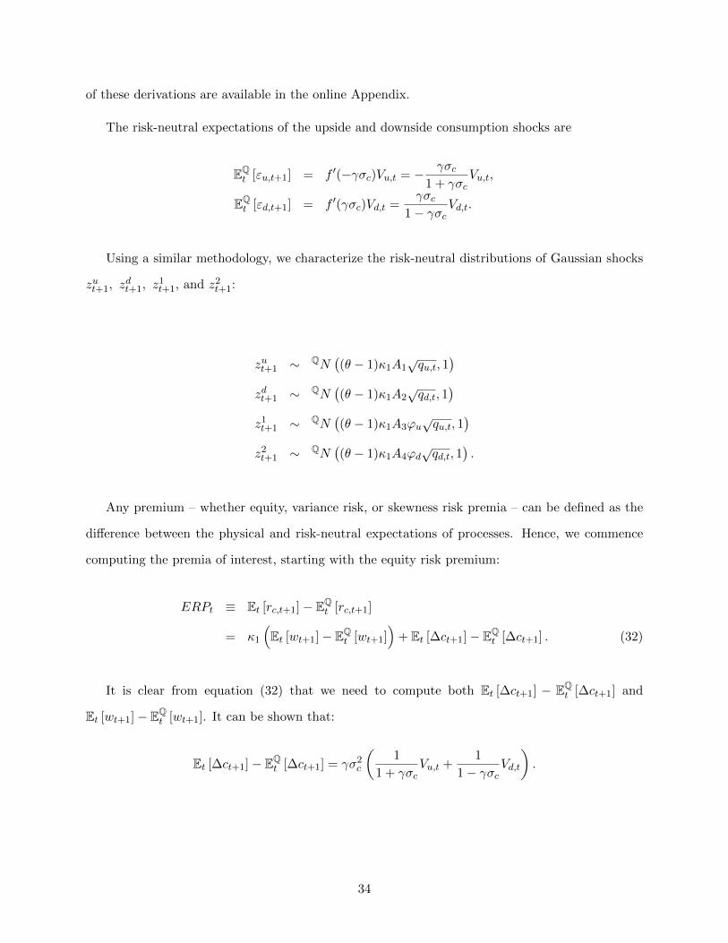
of these derivations are available in the online Appendix.

The risk-neutral expectations of the upside and downside consumption shocks are

EQt [εu,t+1] = f ′(−γσc)Vu,t = − γσc

1 + γσcVu,t,

EQt [εd,t+1] = f ′(γσc)Vd,t =

γσc1− γσc

Vd,t.

Using a similar methodology, we characterize the risk-neutral distributions of Gaussian shocks

zut+1, zdt+1, z

1t+1, and z2

t+1:

zut+1 ∼ QN((θ − 1)κ1A1

√qu,t, 1

)zdt+1 ∼ QN

((θ − 1)κ1A2

√qd,t, 1

)z1t+1 ∼ QN

((θ − 1)κ1A3ϕu

√qu,t, 1

)z2t+1 ∼ QN

((θ − 1)κ1A4ϕd

√qd,t, 1

).

Any premium – whether equity, variance risk, or skewness risk premia – can be defined as the

difference between the physical and risk-neutral expectations of processes. Hence, we commence

computing the premia of interest, starting with the equity risk premium:

ERPt ≡ Et [rc,t+1]− EQt [rc,t+1]

= κ1

(Et [wt+1]− EQ

t [wt+1])

+ Et [∆ct+1]− EQt [∆ct+1] . (32)

It is clear from equation (32) that we need to compute both Et [∆ct+1] − EQt [∆ct+1] and

Et [wt+1]− EQt [wt+1]. It can be shown that:

Et [∆ct+1]− EQt [∆ct+1] = γσ2

c

(1

1 + γσcVu,t +

1

1− γσcVd,t

).

34

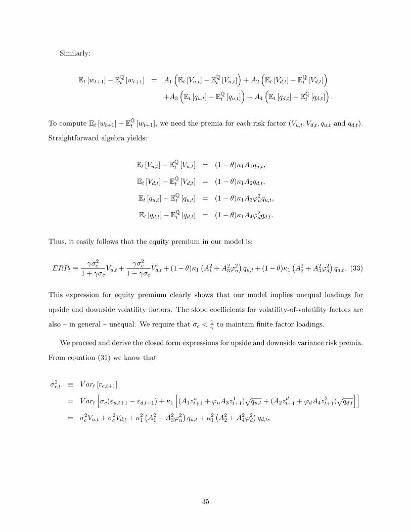
Similarly:

Et [wt+1]− EQt [wt+1] = A1

(Et [Vu,t]− EQ

t [Vu,t])

+A2

(Et [Vd,t]− EQ

t [Vd,t])

+A3

(Et [qu,t]− EQ

t [qu,t])

+A4

(Et [qd,t]− EQ

t [qd,t]).

To compute Et [wt+1]− EQt [wt+1], we need the premia for each risk factor (Vu,t, Vd,t, qu,t and qd,t).

Straightforward algebra yields:

Et [Vu,t]− EQt [Vu,t] = (1− θ)κ1A1qu,t,

Et [Vd,t]− EQt [Vd,t] = (1− θ)κ1A2qd,t,

Et [qu,t]− EQt [qu,t] = (1− θ)κ1A3ϕ

2uqu,t,

Et [qd,t]− EQt [qd,t] = (1− θ)κ1A4ϕ

2dqd,t.

Thus, it easily follows that the equity premium in our model is:

ERPt ≡γσ2

c

1 + γσcVu,t +

γσ2c

1− γσcVd,t + (1− θ)κ1

(A2

1 +A23ϕ

2u

)qu,t + (1− θ)κ1

(A2

2 +A24ϕ

2d

)qd,t. (33)

This expression for equity premium clearly shows that our model implies unequal loadings for

upside and downside volatility factors. The slope coefficients for volatility-of-volatility factors are

also – in general – unequal. We require that σc <1γ to maintain finite factor loadings.

We proceed and derive the closed form expressions for upside and downside variance risk premia.

From equation (31) we know that

σ2r,t ≡ V art [rc,t+1]

= V art

[σc(εu,t+1 − εd,t+1) + κ1

[(A1z

ut+1 + ϕuA3z

1t+1)√qu,t + (A2z

dt+1 + ϕdA4z

2t+1)√qd,t

]]= σ2

cVu,t + σ2cVd,t + κ2

1

(A2

1 +A23ϕ

2u

)qu,t + κ2

1

(A2

2 +A24ϕ

2d

)qd,t,

35

where upside and downside variances are defined as:

(σur,t)2

= σ2cVu,t + κ2

1

(A2

1 +A23ϕ

2u

)qu,t, (34)(

σdr,t

)2= σ2

cVd,t + κ21

(A2

2 +A24ϕ

2d

)qd,t. (35)

Using the definition of variance risk premium, we compute the upside variance risk premium as:

V RPUt ≡ EQt

[(σur,t+1

)2]− Et[(σur,t+1

)2],

= (θ − 1)(σ2cκ1A1 + κ3

1

(A2

1 +A23ϕ

2u

)A3ϕ

2u

)qu,t. (36)

Similarly, we derive the following expression for the downside variance risk premium:

V RPDt ≡ EQt

[(σdr,t+1

)2]− Et

[(σdr,t+1

)2]

= (θ − 1)(σ2cκ1A2 + κ3

1

(A2

2 +A24ϕ

2d

)A4ϕ

2d

)qd,t. (37)

Empirical evidences, presented in Section 4.4, imply V RPUt < 0 and V RPDt > 0, hence it

follows that

σ2cκ1A1 + κ3

1

(A2

1 +A23ϕ

2u

)A3ϕ

2u > 0, (38)

σ2cκ1A2 + κ3

1

(A2

2 +A24ϕ

2d

)A4ϕ

2d < 0. (39)

Since A4 < 0, A2 < 0 is a sufficient condition for σ2cκ1A2 + κ3

1

(A2

2 +A24ϕ

2d

)A4ϕ

2d < 0. Moreover,

A2 < 0⇔ µ2 <

f

[−σc(1−γ)

]γ−1 . In particular, µ2 ≤ 0⇒ A2 < 0⇒ V RP dt > 0. Since A3 < 0, A1 > 0

is a necessary condition for σ2cκ1A1 + κ3

1

(A2

1 +A23ϕ

2u

)A3ϕ

2u > 0. It is easily shown that

σ2cκ1A1 + κ3

1

(A2

1 +A23ϕ

2u

)A3ϕ

2u > 0⇔ AL1 < A1 < AU1

with

AL1 =−σ2

cκ1 +√σ4cκ

21 − 4

(κ3

1A3ϕ2u

)2A2

3ϕ2u

2κ31A3ϕ2

u

, AU1 =−σ2

cκ1 −√σ4cκ

21 − 4

(κ3

1A3ϕ2u

)2A2

3ϕ2u

2κ31A3ϕ2

u

.

36

Both AU1 and AL1 are positive. In addition, it is easy to see that

AL1 < A1 < AU1 ⇔ AL1 < −f

[σc(1− γ)

]+ (1− γ)µ1

θ(κ1βu − 1)< AU1 ,

AL1 < A1 < AU1 ⇔ µL1 < µ1 < µU1 ,

with

µL1 =

f

[σc(1− γ)

]+ θ(κ1βu − 1)AL1

γ − 1> 0,

µU1 =

f

[σc(1− γ)

]+ θ(κ1βu − 1)AU1

γ − 1> 0,

which implies

µ1 > 0.

Consequently, confirming our earlier intuition, we find that for upside variance risk-premium to

be negative, expected consumption growth must increases with the upside variance. Similarly, a

non-positive relation between expected consumption growth and downside variance is sufficient to

induce a positive downside variance risk-premium.

Next, we derive the closed form expression for the skewness risk premium. Following Feunou,

Jahan-Parvar, and Tedongap (2013, 2014), we define the skewness as

skr,t =(σur,t)2 − (σdr,t)2

.

As a result, we calculate the skewness risk premium as

SRPt ≡ V RP ut − V RP dt

=[EQt

[(σur,t+1

)2]− Et[(σur,t+1

)2]]− [EQt

[(σdr,t+1

)2]− Et

[(σdr,t+1

)2]],

= (θ − 1)[(σ2cκ1A1 + κ3

1

(A2

1 +A23ϕ

2u

)A3ϕ

2u

)qu,t −

(σ2cκ1A2 + κ3

1

(A2

2 +A24ϕ

2d

)A4ϕ

2d

)qd,t].(40)

Based on our theoretical findings so far, it is easy to see that given θ < 0 and conditions (38)

37

and (39) – which we just verified – skewness risk premium is negative-valued, in compliance with

our empirical findings in Section 4 and in Figure 7. Finally, since equation (33) implies that the

equity risk-premium load positively on both qu,t and qd,t, and because V RPUt < 0 is negatively

proportional to qu,t and V RPDt > 0 is positively proportional to qd,t, the equity risk-premium

load positively on the downside variance risk-premium and negatively on the upside variance risk-

premium, in compliance with our empirical findings in Section 4 and in Table 9. At this point, we

have fully characterized the equity risk premium, upside and downside variance risk premia, the

skewness risk premium, and by extension, risky asset returns.

In a nutshell, we show that first, our empirical findings are naturally aligned with a simple

consumption-based asset pricing model. Second, the assumptions needed to support our empirical

results are mild – we require distinct and time-varying upside and downside shocks to the consump-

tion growth process, a predictable component in conditional consumption growth proportional to

these up and down shocks variances, and an affine loading on risk factors. These are commonly

maintained assumptions in the variance risk premium literature. Given these assumptions, we show

that the upside variance risk premium is smaller in absolute term than the downside variance risk

premium, that both upside and downside variance risk premia have opposite signs, and that the

skewness risk premium is a negative-valued quantity.

6 Conclusion

In this study, we have decomposed the celebrated variance risk premium of Bollerslev, Tauchen, and

Zhou (2009) – arguably one of the most successful short-term predictors of excess equity returns

– to show that its prediction power stems from the downside variance risk premium embedded in

this measure. Market participants seem more concerned with market downturns and demand a

premium for bearing that risk. By contrast, they seem to like upward uncertainty in the market.

As a result, the downside variance risk premium – the difference between option-implied, risk-

neutral expectations of market downside volatility and historical, realized downside variances –

demonstrates significant prediction power (that is at least as powerful as the variance risk premium

and often stronger) for excess returns.

We also show that the difference between upside and downside variance risk premia – our

38

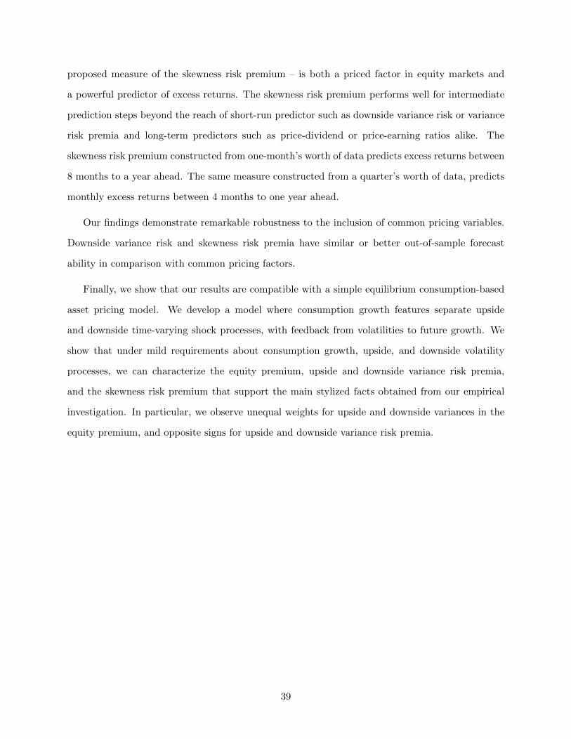
proposed measure of the skewness risk premium – is both a priced factor in equity markets and

a powerful predictor of excess returns. The skewness risk premium performs well for intermediate

prediction steps beyond the reach of short-run predictor such as downside variance risk or variance

risk premia and long-term predictors such as price-dividend or price-earning ratios alike. The

skewness risk premium constructed from one-month’s worth of data predicts excess returns between

8 months to a year ahead. The same measure constructed from a quarter’s worth of data, predicts

monthly excess returns between 4 months to one year ahead.

Our findings demonstrate remarkable robustness to the inclusion of common pricing variables.

Downside variance risk and skewness risk premia have similar or better out-of-sample forecast

ability in comparison with common pricing factors.

Finally, we show that our results are compatible with a simple equilibrium consumption-based

asset pricing model. We develop a model where consumption growth features separate upside

and downside time-varying shock processes, with feedback from volatilities to future growth. We

show that under mild requirements about consumption growth, upside, and downside volatility

processes, we can characterize the equity premium, upside and downside variance risk premia,

and the skewness risk premium that support the main stylized facts obtained from our empirical

investigation. In particular, we observe unequal weights for upside and downside variances in the

equity premium, and opposite signs for upside and downside variance risk premia.

39

References

Amaya, D., P. Christoffersen, K. Jacobs, and A. Vasquez. 2013. Does realized skewness predictthe cross-section of equity returns? Working Paper, UQAM, Rotman School of Management- University of Toronto, C.T. Bauer College of Business - University of Houston, and ITAMSchool of Business .

Amengual, D., and D. Xiu. 2014. Resoution of policy uncertainty and sudden declines in volatility.Working Paper, CEMFI and Chicago Booth .

Andersen, T. G., T. Bollerslev, F. X. Diebold, and H. Ebens. 2001a. The distribution of realizedstock return volatility. Journal of Financial Economics 61:43–76.

Andersen, T. G., T. Bollerslev, F. X. Diebold, and P. Labys. 2001b. The distribution of realizedexchange rate volatility. Journal of the American Statistical Association 96:42–55.

———. 2003. Modeling and forecasting realized volatility. Econometrica 71:579–625.

Andersen, T. G., and O. Bondarenko. 2007. Volatility as an asset class, chap. Construction andInterpretation of Model-Free Implied Volatility, 141–81. London, U.K.: Risk Books.

Andersen, T. G., O. Bondarenko, and M. T. Gonzalez-Perez. 2014. Exploring return dynamics viacorridor implied volatility. Working Paper .

Ang, A., and G. Bekaert. 2007. Stock return predictability: Is it there? Review of Financial Studies20:651–707.

Bakshi, G., N. Kapadia, and D. Madan. 2003. Stock return characteristics, skew laws and thedifferential pricing of individual equity options. Review of Financial Studies 16:101–43.

Bandi, F. M., and R. Reno. 2014. Price and volatility co-jumps. Journal of Financial Economics,forthcoming .

Bansal, R., and A. Yaron. 2004. Risks for the long run: A potential resolution of asset pricingpuzzles. Journal of Finance 59:1481–1509.

Barndorff-Nielsen, O. E., S. Kinnebrock, and N. Shephard. 2010. Volatility and time series econo-metrics: Essays in honor of robert f. engle, chap. Measuring downside risk: realised semivariance,117–36. Oxford University Press.

Bekaert, G., E. Engstrom, and A. Ermolov. 2014. Bad environments, good environments: A non-gaussian asymmetric volatility model. Journal of Econometrics, forthcoming .

Bollerslev, T., G. Tauchen, and H. Zhou. 2009. Expected stock returns and variance risk premia.Review of Financial Studies 22:4463–92.

Bollerslev, T., and V. Todorov. 2011a. Estimation of jump tails. Econometrica 79:1727–83.

———. 2011b. Tails, fears and risk premia. Journal of Finance 66:2165–211.

Boyer, M. M., E. Jacquier, and S. van Norden. 2012. Are underwriting cycles real and forecastable?The Journal of Risk and Insurance 79:995–1015.

Campbell, J. Y., and R. J. Shiller. 1988. The dividend-price ratio and expectations of futuredividends and discount factors. Review of Financial Studies 1:195–228.

40

Carr, P., and D. Madan. 1998. Volatility, chap. Towards a Theory of Volatility Trading, 417–27.Risk Publications.

———. 1999. Option valuation using the fast fourier transform. Journal of Computational Finance2:61–73.

———. 2001. Quantitative analysis of financial markets, vol. 2, chap. Determining Volatility Sur-faces and Option Values from an Implied Volatility Smile, 163–91. World Scientific Press.

Chang, B., P. Christoffersen, and K. Jacobs. 2013. Market skewness risk and the cross-section ofstock returns. Journal of Financial Economics 107:46–68.

Cochrane, J. H. 1991. Production-based asset pricing and the link between stock returns andeconomic fluctuations. Journal of Finance 46:209–37.

Colacito, R., E. Ghysels, and J. Meng. 2014. Skewness in expected macro fundamentals and thepredictability of equity returns: Evidence and theory. Working Paper, Kenan Flagler BusinessSchool, UNC Chapel Hill .

Corsi, F. 2009. A simple approximate long-memory model of realized volatility. Journal of FinancialEconometrics 7:174–96.

Diebold, F. X., and R. S. Mariano. 1995. Comapring predictive accuracy. Journal of Business andEconomic Statistics 13:253–63.

Dionne, G., J. Li, and C. Okou. 2014. An extension of the consumption-based CAPM model.Working Paper, HEC Montreal, Lingnan University, and UQAM .

Drechsler, I., and A. Yaron. 2011. Whats Vol got to do with it? Review of Financial Studies24:1–45.

Eeckhoudt, L., and H. Schlesinger. 2008. Changes in risk and the demand for saving. Journal ofMonetary Economics 55:1329 – 1336.

Epstein, L. G., and S. E. Zin. 1989. Substitution, risk aversion, and the temporal behavior ofconsumption and asset returns: A theoretical framework. Econometrica 57:937–69.

Fama, E. F., and K. R. French. 1988. Dividend yields and expected stock returns. Journal ofFinancial Economics 22:3–25.

———. 1989. Business conditions and expected returns on stocks and bonds. Journal of FinancialEconomics 25:23–49.

Feunou, B., J.-S. Fontaine, A. Taamouti, and R. Tedongap. 2014. Risk premium, variance premium,and the maturity structure of uncertainty. Review of Finance 18:219–69.

Feunou, B., M. R. Jahan-Parvar, and R. Tedongap. 2013. Modeling Market Downside Volatility.Review of Finance 17:443–81.

———. 2014. Which parametric model for conditional skewness? European Journal of Finance,forthcoming .

Ghysels, E., A. Plazzi, and R. Valkanov. 2011. Conditional Skewness of Stock Market Returnsin Developed and Emerging Markets and its Economic Fundamentals. Working Paper, Kenan-Flagler Business School-UNC, and Rady School of Business-UCSD .

41

Gilchrist, S., R. Schoenle, J. W. Sim, and E. Zakrajsek. 2014. Inflation dynamics during thefinancial crisis. Working Paper, Federal Reserve Board and Boston University .

Goyal, A., and I. Welch. 2008. A comprehensive look at the empirical performance of equitypremium prediction. Review of Financial Studies 21:1455–508.

Groeneveld, R., and G. Meeden. 1984. Measuring skewness and kurtosis. The Statistician 33:391–9.

Gul, F. 1991. A Teory of Disappointment Aversion. Econometrica 59:667–86.

Hansen, P. R., and A. Lunde. 2006. Realized variance and market microstructure noise. Journalof Business and Economic Statistics 24:127–61.

Harvey, C. R., and A. Siddique. 1999. Autoregressive Conditional Skewness. Journal of Financialand Quantitative Analysis 34:465–88.

———. 2000. Conditional Skewness in Asset Pricing Tests. Journal of Finance 55:1263–95.

Hodrick, R. J. 1992. Dividend yields and expected stock returns: Alternative procedures forinference and measurement. Review of Financial Studies 5:357–386.

Inoue, A., and L. Kilian. 2004. In-sample or out-of-sample tests of predictability: Which one shouldfwe use? Econometric Reviews 23:371–402.

Jacquier, E., and C. Okou. 2014. Disentangling continuous volatility from jumps in long-run risk-return relationships. Journal of Financial Econometrics 12:544–83.

Kelly, B. T., and H. Jiang. 2014. Tail risk and asset prices. Review of Financial Studies 27:2841–71.

Kelly, B. T., and S. Pruitt. 2013. Market expectations in the cross section of present values. Journalof Finance 68:1721–56.

Kim, T.-H., and H. White. 2004. On More Robust Estimation of Skewness and Kurtosis. FinanceResearch Letters 1:56–73.

Klibanoff, P., M. Marinacci, and S. Mukerji. 2009. Recursive smooth ambiguity preferences. Journalof Economic Theory 144:930–76.

Kozhan, R., A. Neuberger, and P. Schneider. 2014. The skew risk premium in the equity indexmarket. Review of Financial Studies 26:2174–203.

Kreps, D. M., and E. L. Porteus. 1978. Temporal Resolution of Uncertainty and Dynamic ChoiceTheory. Econometrica 46:185–200.

Lettau, M., and S. Ludvigson. 2001. Consumption, aggregate wealth, and expected stock returns.Journal of Finance 56:815–50.

Ludvigson, S. C., and S. Ng. 2009. Macro factors in bond risk premia. Review of Financial Studies22:5027–67.

Miao, J., B. Wei, and H. Zhou. 2012. Ambiguity aversion and variance premium. Working Paper,Federal Reserve Board and Boston University .

Nakamura, E., J. Steinsson, R. Barro, and J. Ursua. 2013. Crises and recoveries in an empiricalmodel of consumption disasters. American Economic Journal: Macroeconomics 5:35–74.

42

Neuberger, A. 2012. Realized skewness. Review of Financial Studies 25:3423–55.

Segal, G., I. Shaliastovich, and A. Yaron. 2015. Good and bad uncertainty: Macroeconomic andfinancial market implications. Journal of Financial Economics, forthcoming .

Weil, P. 1989. The equity premium puzzle and the risk-free rate puzzle. Journal of MonetaryEconomics 24:401–21.

West, K. D. 1996. Asymptotic inference about predictive ability. Econometrica 64:1067–84.

43

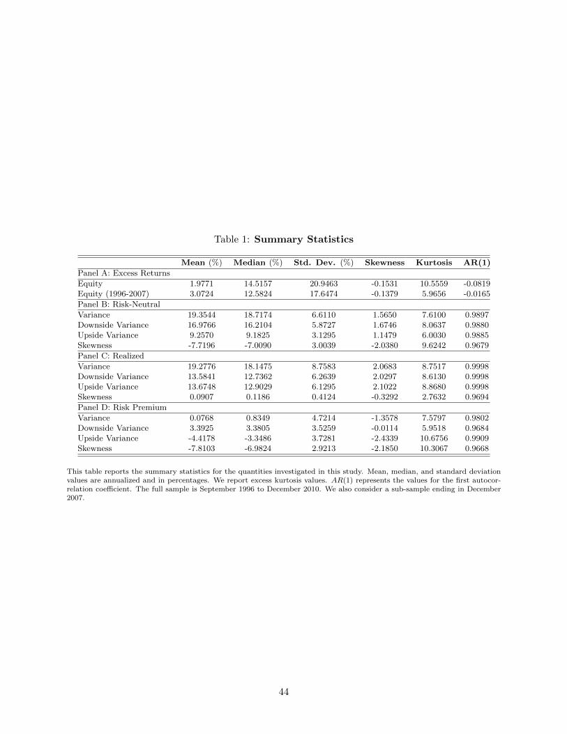
Table 1: Summary Statistics

Mean (%) Median (%) Std. Dev. (%) Skewness Kurtosis AR(1)

Panel A: Excess Returns

Equity 1.9771 14.5157 20.9463 -0.1531 10.5559 -0.0819Equity (1996-2007) 3.0724 12.5824 17.6474 -0.1379 5.9656 -0.0165

Panel B: Risk-Neutral

Variance 19.3544 18.7174 6.6110 1.5650 7.6100 0.9897Downside Variance 16.9766 16.2104 5.8727 1.6746 8.0637 0.9880Upside Variance 9.2570 9.1825 3.1295 1.1479 6.0030 0.9885Skewness -7.7196 -7.0090 3.0039 -2.0380 9.6242 0.9679

Panel C: Realized

Variance 19.2776 18.1475 8.7583 2.0683 8.7517 0.9998Downside Variance 13.5841 12.7362 6.2639 2.0297 8.6130 0.9998Upside Variance 13.6748 12.9029 6.1295 2.1022 8.8680 0.9998Skewness 0.0907 0.1186 0.4124 -0.3292 2.7632 0.9694

Panel D: Risk Premium

Variance 0.0768 0.8349 4.7214 -1.3578 7.5797 0.9802Downside Variance 3.3925 3.3805 3.5259 -0.0114 5.9518 0.9684Upside Variance -4.4178 -3.3486 3.7281 -2.4339 10.6756 0.9909Skewness -7.8103 -6.9824 2.9213 -2.1850 10.3067 0.9668

This table reports the summary statistics for the quantities investigated in this study. Mean, median, and standard deviationvalues are annualized and in percentages. We report excess kurtosis values. AR(1) represents the values for the first autocor-relation coefficient. The full sample is September 1996 to December 2010. We also consider a sub-sample ending in December2007.

44

Table 2: S&P 500 Index Option Data

OTM Put OTM Call

S/S<

0.9

7

0.9

7<

S/S<

0.9

9

0.9

9<

S/S<

1.0

1

1.0

1<

S/S<

1.0

3

1.0

3<

S/S<

1.0

5

S/S>

1.0

5

All

Panel A: By Moneyness

Number of contracts 223,579 57,188 71,879 57,522 26,154 100,121 536,443Average price 15.08 39.44 39.67 38.47 21.97 15.50 23.90Average implied volatility 25.68 17.05 15.88 15.58 14.30 16.31 20.06

DT

M<

30

30<

DT

M<

60

60<

DT

M<

90

90<

DT

M<

120

120<

DT

M<

150

DT

M>

150

All

Panel B: By Maturity

Number of contracts 115,392 140,080 83,937 36,163 22,302 138,569 536,443Average price 10.45 14.90 20.17 24.88 26.20 45.82 23.90Average implied volatility 19.40 20.20 20.06 21.11 20.48 20.13 20.06

VIX

<15

15<

VIX

<20

20<

VIX

<25

25<

VIX

<30

30<

VIX

<35

VIX

>35

All

Panel C: By VIX Level

Number of contracts 74,048 115,970 164,832 88,146 37,008 56,439 536,443Average price 17.90 20.70 24.89 26.84 26.80 28.93 23.90Average implied volatility 11.63 15.92 19.42 22.20 25.31 34.72 20.06

This table sorts S&P 500 index option data by moneyness, maturity, and VIX level. Out-of-the-money (OTM) call and putoptions from OptionMetrics from September 3, 1996 to December 30, 2010 are used. The moneyness is measured by the ratioof the strike price (S) to underlying asset price (S). DTM is the time to maturity in number of calendar days. The averageprice and the average implied volatility are expressed in dollars and percentages, respectively.

45

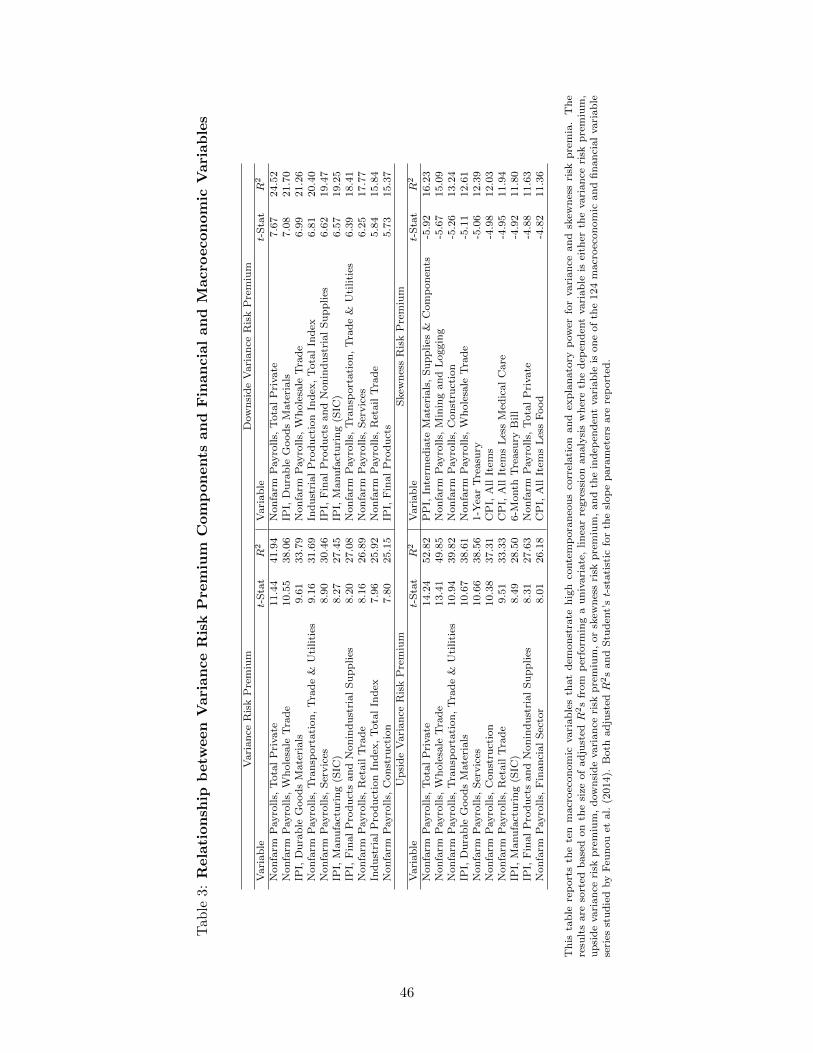
Tab

le3:

Rela

tion

ship

betw

een

Vari

an

ce

Ris

kP

rem

ium

Com

pon

ents

an

dF

inan

cia

lan

dM

acro

econom

icV

ari

ab

les

Vari

an

ceR

isk

Pre

miu

mD

ow

nsi

de

Vari

an

ceR

isk

Pre

miu

mV

ari

ab

let-

Sta

tR

2V

ari

ab

let-

Sta

tR

2

Non

farm

Payro

lls,

Tota

lP

rivate

11.4

441.9

4N

on

farm

Payro

lls,

Tota

lP

rivate

7.6

724.5

2N

on

farm

Payro

lls,

Wh

ole

sale

Tra

de

10.5

538.0

6IP

I,D

ura

ble

Good

sM

ate

rials

7.0

821.7

0IP

I,D

ura

ble

Good

sM

ate

rials

9.6

133.7

9N

on

farm

Payro

lls,

Wh

ole

sale

Tra

de

6.9

921.2

6N

on

farm

Payro

lls,

Tra

nsp

ort

ati

on

,T

rad

e&

Uti

liti

es9.1

631.6

9In

du

stri

al

Pro

du

ctio

nIn

dex

,T

ota

lIn

dex

6.8

120.4

0N

on

farm

Payro

lls,

Ser

vic

es8.9

030.4

6IP

I,F

inal

Pro

du

cts

an

dN

on

ind

ust

rial

Su

pp

lies

6.6

219.4

7IP

I,M

anu

fact

uri

ng

(SIC

)8.2

727.4

5IP

I,M

anu

fact

uri

ng

(SIC

)6.5

719.2

5IP

I,F

inal

Pro

du

cts

an

dN

on

ind

ust

rial

Su

pp

lies

8.2

027.0

8N

on

farm

Payro

lls,

Tra

nsp

ort

ati

on

,T

rad

e&

Uti

liti

es6.3

918.4

1N

on

farm

Payro

lls,

Ret

ail

Tra

de

8.1

626.8

9N

on

farm

Payro

lls,

Ser

vic

es6.2

517.7

7In

du

stri

al

Pro

du

ctio

nIn

dex

,T

ota

lIn

dex

7.9

625.9

2N

on

farm

Payro

lls,

Ret

ail

Tra

de

5.8

415.8

4N

on

farm

Payro

lls,

Con

stru

ctio

n7.8

025.1

5IP

I,F

inal

Pro

du

cts

5.7

315.3

7U

psi

de

Vari

an

ceR

isk

Pre

miu

mS

kew

nes

sR

isk

Pre

miu

mV

ari

ab

let-

Sta

tR

2V

ari

ab

let-

Sta

tR

2

Non

farm

Payro

lls,

Tota

lP

rivate

14.2

452.8

2P

PI,

Inte

rmed

iate

Mate

rials

,S

up

plies

&C

om

pon

ents

-5.9

216.2

3N

on

farm

Payro

lls,

Wh

ole

sale

Tra

de

13.4

149.8

5N

on

farm

Payro

lls,

Min

ing

an

dL

oggin

g-5

.67

15.0

9N

on

farm

Payro

lls,

Tra

nsp

ort

ati

on

,T

rad

e&

Uti

liti

es10.9

439.8

2N

on

farm

Payro

lls,

Con

stru

ctio

n-5

.26

13.2

4IP

I,D

ura

ble

Good

sM

ate

rials

10.6

738.6

1N

on

farm

Payro

lls,

Wh

ole

sale

Tra

de

-5.1

112.6

1N

on

farm

Payro

lls,

Ser

vic

es10.6

638.5

61-Y

ear

Tre

asu

ry-5

.06

12.3

9N

on

farm

Payro

lls,

Con

stru

ctio

n10.3

837.3

1C

PI,

All

Item

s-4

.98

12.0

3N

on

farm

Payro

lls,

Ret

ail

Tra

de

9.5

133.3

3C

PI,

All

Item

sL

ess

Med

ical

Care

-4.9

511.9

4IP

I,M

anu

fact

uri

ng

(SIC

)8.4

928.5

06-M

onth

Tre

asu

ryB

ill

-4.9

211.8

0IP

I,F

inal

Pro

du

cts

an

dN

on

ind

ust

rial

Su

pp

lies

8.3

127.6

3N

on

farm

Payro

lls,

Tota

lP

rivate

-4.8

811.6

3N

on

farm

Payro

lls,

Fin

an

cial

Sec

tor

8.0

126.1

8C

PI,

All

Item

sL

ess

Food

-4.8

211.3

6

Th

ista

ble

rep

ort

sth

ete

nm

acr

oec

on

om

icvari

ab

les

that

dem

on

stra

teh

igh

conte

mp

ora

neo

us

corr

elati

on

an

dex

pla

nato

ryp

ow

erfo

rvari

an

cean

dsk

ewn

ess

risk

pre

mia

.T

he

resu

lts

are

sort

edb

ase

don

the

size

of

ad

just

edR

2s

from

per

form

ing

au

niv

ari

ate

,lin

ear

regre

ssio

nan

aly

sis

wh

ere

the

dep

end

ent

vari

ab

leis

eith

erth

evari

an

ceri

skp

rem

ium

,u

psi

de

vari

an

ceri

skp

rem

ium

,d

ow

nsi

de

vari

an

ceri

skp

rem

ium

,or

skew

nes

sri

skpre

miu

m,

an

dth

ein

dep

end

ent

vari

ab

leis

on

eof

the

124

macr

oec

on

om

ican

dfi

nan

cial

vari

ab

lese

ries

stu

die

dby

Feu

nou

etal.

(2014).

Both

ad

just

edR

2s

an

dS

tud

ent’

st-

stati

stic

for

the

slop

ep

ara

met

ers

are

rep

ort

ed.

46

Tab

le4:

Poli

cy

New

sP

ote

nti

all

yA

ssocia

ted

wit

hV

ola

tili

tyC

han

ges–

Booth

Date

s

Date

∆V

ari

an

ce∆

Ret

urn

New

s

08/18/98

-0.3

73

(-0.3

65)

0.0

13

Pre

sid

ent

Cli

nto

nad

mit

sto

“w

ron

g”

rela

tion

ship

wit

hM

s.L

ewin

sky

an

dF

OM

C’s

dec

isio

nto

leav

ein

tere

stra

tes

un

chan

ged

09/01/98

-0.7

22

(-0.6

64)

0.0

35

Fed

ad

ds

mon

eyto

the

ban

kin

gsy

stem

wit

hR

epo.

09/08/98

-0.5

26

(-0.4

55)

0.0

21

Fed

Ch

air

man

Gre

ensp

an

’sst

ate

men

tth

at

ara

tecu

tm

ight

be

fort

hco

min

g.

09/14/98

-0.1

85

Pre

sid

ent

Cli

nto

nad

voca

ted

aco

ord

inate

dglo

bal

poli

cyfo

rec

on

om

icgro

wth

inN

YC

.09/23/98

-0.3

44

(-0.2

80)

0.0

27

Fed

Ch

air

man

Gre

ensp

an

test

imony

bef

ore

the

Com

mit

tee

on

the

Bu

dget

,U

.S.

Sen

ate

.10/20/98

-0.2

53

-0.0

07

3b

igU

Sb

an

ks

del

iver

edb

ette

r-th

an

-exp

ecte

dea

rnin

gs

an

db

ull

ish

mood

aft

erF

edra

tecu

tp

revio

us

wee

k.

08/11/99

-0.2

66

(-0.2

76)

0.0

08

Fed

Bei

ge

Book

rele

ase

show

sth

at

US

econ

om

icgro

wth

rem

ain

sst

ron

g.

01/07/00

-0.5

00

0.0

31

Un

emp

loym

ent

rep

ort

show

sth

elo

wes

tu

nem

plo

ym

ent

rate

inth

ep

ast

30

yea

rs.

03/16/00

-0.2

66

0.0

37

Rel

ease

of

Infl

ati

on

Rem

ain

sT

am

eE

nou

gh

toK

eep

the

Fed

eral

Res

erve

from

Tig

hte

nin

gC

red

it04/17/00

-0.3

73

(-0.2

96)

0.0

32

Tre

asu

ryS

ecre

tary

Law

ren

ceH

.S

um

mer

sS

tate

men

tth

at

Fu

nd

am

enta

lsof

Eco

nom

yare

inP

lace

10/19/00

-0.2

41

0.0

18

Fed

sG

reen

span

Giv

esK

eyn

ote

Sp

eech

at

Cato

Inst

itu

tean

dJob

less

Cla

imD

rop

by

7,0

00

inL

ate

stW

eek

01/03/01

-0.2

82

(-0.1

79)

0.0

52

Fed

’sA

nn

ou

nce

men

tof

aS

urp

rise

,In

ter-

Mee

tin

gR

ate

Cu

t05/17/05

-0.2

75

(-0.3

03)

0.0

1Joh

nS

now

Call

on

Ch

ina

toT

ake

An

Inte

rmed

iate

Ste

pin

Rev

alu

ing

its

Cu

rren

cy05/19/05

-0.2

97

Fed

Ch

air

man

A.

Gre

ensp

an

Ste

ps

up

Cri

tici

smof

Fan

nie

Mae

an

dF

red

die

Mac

06/15/06

-0.5

49

(-0.6

25)

0.0

17

Fed

Ch

air

man

B.

Ber

nan

kes

Sp

eech

on

Infl

ati

on

Exp

ecta

tion

sw

ith

inH

isto

rica

lR

an

ges

06/29/06

-0.2

95

(-0.3

25)

0.0

16

FO

MC

Sta

tem

ent

toR

ais

eIt

sT

arg

etfo

rth

eF

eder

al

Fu

nd

sR

ate

by

25

Basi

sP

oin

ts07/19/06

-0.2

72

Fed

Ch

air

man

B.

Ber

nan

ke

Warn

edth

at

the

Fed

Mu

stG

uard

Again

stR

isin

gP

rice

sT

akin

gH

old

02/28/07

-0.3

96

Fed

Ch

air

man

B.

Ber

nan

ke

Told

aH

ou

seP

an

elth

at

Mark

ets

See

med

Work

ing

Wel

l03/06/07

-0.2

17

Hen

ryP

au

lson

inT

okyo

Said

the

Glo

bal

Eco

nom

yw

as

As

Str

on

gA

sH

e’s

Ever

See

n06/27/07

-0.2

71

FO

MC

An

nou

nce

men

tG

ener

ate

dM

ark

etR

ebou

nd

the

Pre

vio

us

Date

08/21/07

-0.1

88

Sen

ato

rD

od

dsa

idth

eF

edto

Dea

lw

ith

the

Tu

rmoil

aft

erM

eeti

ng

wit

hP

au

lson

an

dB

ern

an

ke

09/18/07

-0.4

15

(-0.3

53)

0.0

24

FO

MC

Dec

ided

toL

ower

its

Targ

etfo

rth

eF

eder

al

Fu

nd

sR

ate

by

50

Basi

sP

oin

ts03/18/08

-0.2

16

Fed

Cu

tth

eF

edF

un

ds

Rate

by

Thre

e-Q

uart

ers

of

aP

erce

nta

ge

Poin

t10/14/08

-0.4

89

(-0.3

04)

-0.0

48

FO

MC

Dec

ided

toL

ower

its

Targ

etfo

rth

eF

eder

al

Fu

nd

sR

ate

by

50

Basi

sP

oin

ts10/20/08

-0.4

26

(-0.4

13)

0.0

33

Fed

Ch

air

man

B.

Ber

nan

ke

Tes

tim

ony

on

the

Bu

dget

,U

.S.

Hou

seof

Rep

rese

nta

tives

10/28/08

-0.3

13

(-0.2

30)

0.0

75

Fed

toC

ut

the

Rate

Foll

owin

gth

eT

wo-D

ayF

OM

CM

eeti

ng

isE

xp

ecte

dby

the

Mark

et11/13/08

-0.3

28

(-0.2

40)

0.0

62

Pre

sid

ent

Bu

sh’s

Sp

eech

on

Fin

an

cial

Cri

sis

12/19/08

-0.2

44

Pre

sid

ent

Bu

shD

ecla

red

that

TA

RP

Fu

nd

sto

be

Sp

ent

on

Pro

gra

ms

Pau

lson

Dee

med

Nec

essa

ry02/24/09

-0.2

61

Pre

sid

ent

Ob

am

a’s

Fir

stS

pee

chas

the

Pre

sid

ent

toJoin

tS

essi

on

of

U.S

.C

on

gre

ss05/10/10

-0.6

47

(-0.6

01)

0.0

03

Eu

rop

ean

Poli

cyM

aker

sU

nvei

led

An

Un

pre

ced

ente

dE

mer

gen

cyL

oan

Pla

n03/21/11

-0.2

77

Jap

an

ese

Nu

clea

rR

eact

ors

Coole

dD

own

an

dS

itu

ati

on

sin

Lib

ya

Tam

edby

Un

ilate

ral

Forc

es08/09/11

-0.4

33

(-0.3

70)

0.0

46

FO

MC

Sta

tem

ent

Exp

lici

tly

Sta

tin

gA

Du

rati

on

for

An

Exce

pti

on

all

yL

owT

arg

etR

ate

10/27/11

-0.2

45

(-0.2

05)

0.0

34

Eu

rop

ean

Un

ion

Lea

der

sM

ad

ea

Bon

dD

eal

toF

ixth

eG

reek

Deb

tC

risi

s01/02/13

-0.4

32

(-0.4

27)

0.0

25

Pre

sid

ent

Ob

am

aan

dS

enato

rM

cCon

nel

l’s

En

cou

ragin

gC

om

men

tson

the

“F

isca

lC

liff

”Is

sue

This

table

from

Am

engual

and

Xiu

(2014)

pre

sents

inth

ela

stcolu

mn

the

events

that

may

lead

toth

ela

rgest

vola

tility

dro

ps

insa

mple

.T

he

firs

tcolu

mn

isth

edate

of

the

event.

The

second

show

schanges

inest

imate

dsp

ot

vari

ance,

where

as

the

thir

dcolu

mn

isth

ere

turn

sof

the

index

on

the

corr

esp

ondin

gdays.

47

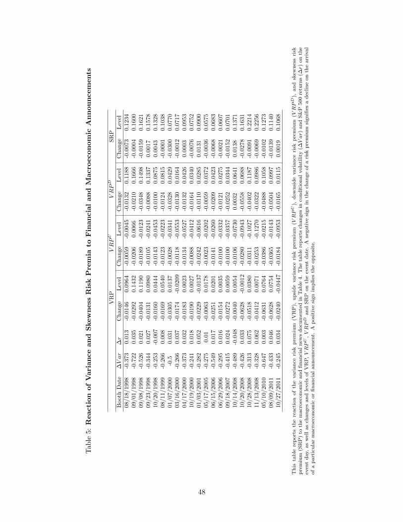
Tab

le5:

Reacti

on

of

Vari

an

ce

an

dS

kew

ness

Ris

kP

rem

iato

Fin

an

cia

lan

dM

acro

econ

om

icA

nn

ou

ncem

ents

VR

PVRPU

VRPD

SR

P

Booth

Date

∆Var

∆r

Change

Lev

elC

hange

Lev

elC

hange

Lev

elC

hange

Lev

el

08/18/1998

-0.3

73

0.0

13

-0.0

146

0.0

964

-0.0

059

-0.0

045

-0.0

132

0.1

188

-0.0

073

0.1

234

09/01/1998

-0.7

22

0.0

35

-0.0

292

0.1

432

-0.0

206

0.0

066

-0.0

210

0.1

666

-0.0

004

0.1

600

09/08/1998

-0.5

26

0.0

21

-0.0

404

0.1

190

-0.0

189

-0.0

123

-0.0

348

0.1

498

-0.0

159

0.1

621

09/23/1998

-0.3

44

0.0

27

-0.0

131

0.0

980

-0.0

105

-0.0

241

-0.0

088

0.1

337

0.0

017

0.1

578

10/20/1998

-0.2

53

-0.0

07

-0.0

160

0.0

444

-0.0

143

-0.0

453

-0.0

100

0.0

875

0.0

043

0.1

328

08/11/1999

-0.2

66

0.0

08

-0.0

169

0.0

540

-0.0

123

-0.0

223

-0.0

124

0.0

815

-0.0

001

0.1

038

01/07/2000

-0.5

0.0

31

-0.0

305

0.0

137

-0.0

028

-0.0

341

-0.0

328

0.0

429

-0.0

300

0.0

770

03/16/2000

-0.2

66

0.0

37

-0.0

174

-0.0

209

-0.0

118

-0.0

553

-0.0

130

0.0

164

-0.0

012

0.0

717

04/17/2000

-0.3

73

0.0

32

-0.0

183

0.0

023

-0.0

134

-0.0

527

-0.0

132

0.0

426

0.0

003

0.0

953

10/19/2000

-0.2

41

0.0

18

-0.0

190

0.0

027

-0.0

088

-0.0

412

-0.0

164

0.0

340

-0.0

076

0.0

752

01/03/2001

-0.2

82

0.0

52

-0.0

229

-0.0

137

-0.0

242

-0.0

616

-0.0

110

0.0

285

0.0

131

0.0

900

05/17/2005

-0.2

75

0.0

1-0

.0063

0.0

178

-0.0

023

-0.0

202

-0.0

059

0.0

372

-0.0

036

0.0

575

06/15/2006

-0.5

49

0.0

17

-0.0

251

0.0

201

-0.0

141

-0.0

260

-0.0

209

0.0

423

-0.0

068

0.0

683

06/29/2006

-0.2

95

0.0

16

-0.0

154

0.0

035

-0.0

100

-0.0

332

-0.0

121

0.0

275

-0.0

021

0.0

607

09/18/2007

-0.4

15

0.0

24

-0.0

272

0.0

059

-0.0

100

-0.0

357

-0.0

252

0.0

344

-0.0

152

0.0

701

10/14/2008

-0.4

89

-0.0

48

-0.0

040

0.0

054

-0.0

106

-0.0

730

0.0

032

0.0

641

0.0

138

0.1

371

10/20/2008

-0.4

26

0.0

33

-0.0

628

-0.0

012

-0.0

280

-0.0

943

-0.0

558

0.0

688

-0.0

278

0.1

631

10/28/2008

-0.3

13

0.0

75

-0.0

518

0.0

380

-0.0

311

-0.1

027

-0.0

402

0.1

187

-0.0

091

0.2

214

11/13/2008

-0.3

28

0.0

62

-0.0

412

0.0

071

-0.0

253

-0.1

270

-0.0

322

0.0

986

-0.0

069

0.2

256

05/10/2010

-0.6

47

0.0

03

-0.0

631

0.0

764

-0.0

386

-0.0

215

-0.0

488

0.1

058

-0.0

102

0.1

273

08/09/2011

-0.4

33

0.0

46

-0.0

628

0.0

754

-0.0

365

-0.0

143

-0.0

504

0.0

997

-0.0

139

0.1

140

10/27/2011

-0.2

45

0.0

34

-0.0

240

-0.0

447

-0.0

184

-0.0

953

-0.0

165

0.0

115

0.0

019

0.1

068

Th

ista

ble

rep

ort

sth

ere

act

ion

of

the

vari

an

ceri

skp

rem

ium

(VR

P),

up

sid

evari

an

ceri

skp

rem

ium

(VRPU

),d

ow

nsi

de

vari

an

ceri

skp

rem

ium

(VRPD

),an

dsk

ewn

ess

risk

pre

miu

m(S

RP

)to

the

macr

oec

on

om

ican

dfi

nan

cial

new

sd

ocu

men

ted

inT

ab

le4.

Th

eta

ble

rep

ort

sch

an

ges

inco

nd

itio

nal

vola

tility

(∆Var)

an

dS

&P

500

retu

rns

(∆r)

on

the

even

td

ay,

as

wel

las

chan

ges

an

dle

vel

sof

VR

P,VRPU

,VRPD

an

dS

RP

on

the

even

td

ate

.A

neg

ati

ve

sign

inth

ech

an

ge

of

ari

skp

rem

ium

sign

ifies

ad

eclin

eon

the

arr

ival

of

ap

art

icu

lar

macr

oec

on

om

icor

fin

an

cial

an

nou

nce

men

t.A

posi

tive

sign

imp

lies

the

op

posi

te.

48

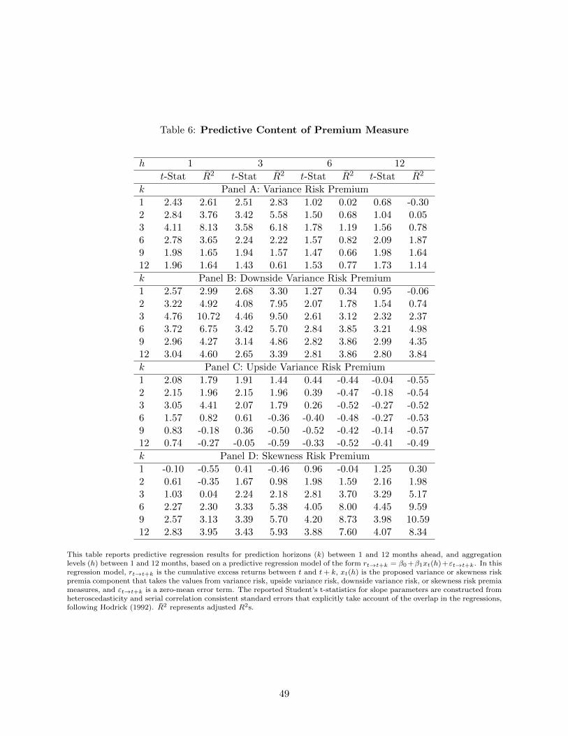
Table 6: Predictive Content of Premium Measure

h 1 3 6 12

t-Stat R2 t-Stat R2 t-Stat R2 t-Stat R2

k Panel A: Variance Risk Premium

1 2.43 2.61 2.51 2.83 1.02 0.02 0.68 -0.302 2.84 3.76 3.42 5.58 1.50 0.68 1.04 0.053 4.11 8.13 3.58 6.18 1.78 1.19 1.56 0.786 2.78 3.65 2.24 2.22 1.57 0.82 2.09 1.879 1.98 1.65 1.94 1.57 1.47 0.66 1.98 1.6412 1.96 1.64 1.43 0.61 1.53 0.77 1.73 1.14

k Panel B: Downside Variance Risk Premium

1 2.57 2.99 2.68 3.30 1.27 0.34 0.95 -0.062 3.22 4.92 4.08 7.95 2.07 1.78 1.54 0.743 4.76 10.72 4.46 9.50 2.61 3.12 2.32 2.376 3.72 6.75 3.42 5.70 2.84 3.85 3.21 4.989 2.96 4.27 3.14 4.86 2.82 3.86 2.99 4.3512 3.04 4.60 2.65 3.39 2.81 3.86 2.80 3.84

k Panel C: Upside Variance Risk Premium

1 2.08 1.79 1.91 1.44 0.44 -0.44 -0.04 -0.552 2.15 1.96 2.15 1.96 0.39 -0.47 -0.18 -0.543 3.05 4.41 2.07 1.79 0.26 -0.52 -0.27 -0.526 1.57 0.82 0.61 -0.36 -0.40 -0.48 -0.27 -0.539 0.83 -0.18 0.36 -0.50 -0.52 -0.42 -0.14 -0.5712 0.74 -0.27 -0.05 -0.59 -0.33 -0.52 -0.41 -0.49

k Panel D: Skewness Risk Premium

1 -0.10 -0.55 0.41 -0.46 0.96 -0.04 1.25 0.302 0.61 -0.35 1.67 0.98 1.98 1.59 2.16 1.983 1.03 0.04 2.24 2.18 2.81 3.70 3.29 5.176 2.27 2.30 3.33 5.38 4.05 8.00 4.45 9.599 2.57 3.13 3.39 5.70 4.20 8.73 3.98 10.5912 2.83 3.95 3.43 5.93 3.88 7.60 4.07 8.34

This table reports predictive regression results for prediction horizons (k) between 1 and 12 months ahead, and aggregationlevels (h) between 1 and 12 months, based on a predictive regression model of the form rt→t+k = β0 +β1xt(h)+εt→t+k. In thisregression model, rt→t+k is the cumulative excess returns between t and t+ k, xt(h) is the proposed variance or skewness riskpremia component that takes the values from variance risk, upside variance risk, downside variance risk, or skewness risk premiameasures, and εt→t+k is a zero-mean error term. The reported Student’s t-statistics for slope parameters are constructed fromheteroscedasticity and serial correlation consistent standard errors that explicitly take account of the overlap in the regressions,following Hodrick (1992). R2 represents adjusted R2s.

49

Table 7: Predictive Content of Risk-Neutral Measure

h 1 3 6 12

t-Stat R2 t-Stat R2 t-Stat R2 t-Stat R2

k Panel A: Risk-Neutral Variance

1 0.28 -0.51 0.50 -0.41 0.69 -0.29 0.75 -0.242 1.14 0.17 1.24 0.30 1.35 0.44 1.39 0.513 1.30 0.38 1.52 0.72 1.83 1.28 2.13 1.926 2.10 1.88 2.33 2.43 2.76 3.57 3.21 4.959 2.32 2.44 2.55 3.05 2.95 4.22 3.15 4.8512 2.21 2.20 2.45 2.82 2.89 4.11 3.30 5.45

k Panel B: Risk-Neutral Downside Variance

1 0.27 -0.51 0.57 -0.37 0.77 -0.23 0.87 -0.142 1.22 0.27 1.39 0.51 1.49 0.66 1.54 0.743 1.42 0.56 1.70 1.04 2.03 1.70 2.35 2.446 2.23 2.17 2.52 2.91 2.97 4.21 3.42 5.679 2.43 2.71 2.68 3.42 3.10 4.70 3.26 5.2212 2.32 2.48 2.55 3.09 2.99 4.42 3.42 5.84

k Panel C: Risk-Neutral Upside Variance

1 0.29 -0.50 0.27 -0.51 0.36 -0.48 0.20 -0.532 0.93 -0.07 0.76 -0.23 0.78 -0.21 0.60 -0.353 0.99 -0.02 0.94 -0.06 1.04 0.05 1.00 0.006 1.74 1.12 1.72 1.09 1.92 1.48 2.05 1.779 2.01 1.71 2.09 1.89 2.31 2.42 2.38 2.5912 1.90 1.49 2.09 1.92 2.45 2.83 2.57 3.17

k Panel D: Risk-Neutral Skewness

1 0.22 -0.52 0.87 -0.14 1.10 0.11 1.27 0.342 1.51 0.70 2.02 1.67 2.06 1.76 2.08 1.793 1.93 1.48 2.47 2.74 2.85 3.80 3.13 4.656 2.70 3.42 3.28 5.21 3.80 7.02 4.11 8.189 2.76 3.64 3.17 4.92 3.64 6.54 3.56 6.2612 2.67 3.44 2.88 4.07 3.27 5.35 3.66 6.73

This table reports predictive regression results for risk-neutral variance and skewness measures. The predictive regression model,prediction horizons, aggregation levels, and notation are the same as in the results reported in Table 6. The difference is in thedefinition of xt(h): instead of risk premia, we use risk-neutral measures for variance, upside variance, downside variance, andskewness.

50

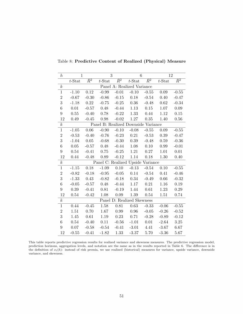
Table 8: Predictive Content of Realized (Physical) Measure

h 1 3 6 12

t-Stat R2 t-Stat R2 t-Stat R2 t-Stat R2

k Panel A: Realized Variance

1 -1.10 0.12 -0.99 -0.01 -0.10 -0.55 0.09 -0.552 -0.67 -0.30 -0.86 -0.15 0.18 -0.54 0.40 -0.473 -1.18 0.22 -0.75 -0.25 0.36 -0.48 0.62 -0.346 0.01 -0.57 0.48 -0.44 1.13 0.15 1.07 0.099 0.55 -0.40 0.78 -0.22 1.33 0.44 1.12 0.1512 0.49 -0.45 0.98 -0.02 1.27 0.35 1.40 0.56

k Panel B: Realized Downside Variance

1 -1.05 0.06 -0.90 -0.10 -0.08 -0.55 0.09 -0.552 -0.53 -0.40 -0.76 -0.23 0.21 -0.53 0.39 -0.473 -1.04 0.05 -0.68 -0.30 0.39 -0.48 0.59 -0.366 0.05 -0.57 0.48 -0.44 1.08 0.10 0.99 -0.019 0.54 -0.41 0.75 -0.25 1.21 0.27 1.01 0.0112 0.44 -0.48 0.89 -0.12 1.14 0.18 1.30 0.40

k Panel C: Realized Upside Variance

1 -1.15 0.18 -1.09 0.10 -0.13 -0.54 0.10 -0.552 -0.82 -0.18 -0.95 -0.05 0.14 -0.54 0.41 -0.463 -1.33 0.43 -0.82 -0.18 0.34 -0.49 0.66 -0.326 -0.05 -0.57 0.48 -0.44 1.17 0.21 1.16 0.199 0.39 -0.41 0.81 -0.19 1.44 0.61 1.23 0.2912 0.54 -0.42 1.08 0.09 1.39 0.54 1.51 0.74

k Panel D: Realized Skewness

1 0.44 -0.45 1.58 0.81 0.63 -0.33 -0.06 -0.552 1.51 0.70 1.67 0.99 0.96 -0.05 -0.26 -0.523 1.45 0.61 1.19 0.23 0.71 -0.28 -0.89 -0.126 0.54 -0.40 0.11 -0.56 -1.01 0.01 -2.64 3.259 0.07 -0.58 -0.54 -0.41 -3.01 4.41 -3.67 6.6712 -0.55 -0.41 -1.82 1.33 -3.37 5.70 -3.36 5.67

This table reports predictive regression results for realized variance and skewness measures. The predictive regression model,prediction horizons, aggregation levels, and notation are the same as in the results reported in Table 6. The difference is inthe definition of xt(h): instead of risk premia, we use realized (historical) measures for variance, upside variance, downsidevariance, and skewness.

51

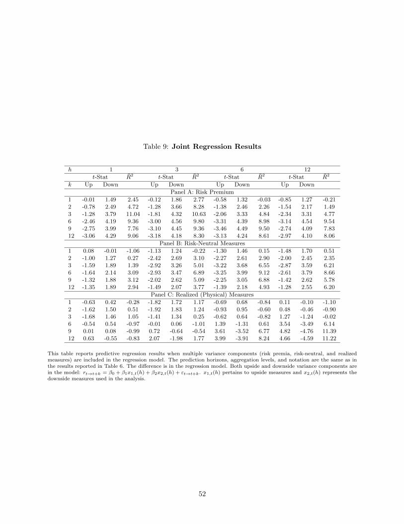
Table 9: Joint Regression Results

h 1 3 6 12

t-Stat R2 t-Stat R2 t-Stat R2 t-Stat R2

k Up Down Up Down Up Down Up Down

Panel A: Risk Premium

1 -0.01 1.49 2.45 -0.12 1.86 2.77 -0.58 1.32 -0.03 -0.85 1.27 -0.212 -0.78 2.49 4.72 -1.28 3.66 8.28 -1.38 2.46 2.26 -1.54 2.17 1.493 -1.28 3.79 11.04 -1.81 4.32 10.63 -2.06 3.33 4.84 -2.34 3.31 4.776 -2.46 4.19 9.36 -3.00 4.56 9.80 -3.31 4.39 8.98 -3.14 4.54 9.549 -2.75 3.99 7.76 -3.10 4.45 9.36 -3.46 4.49 9.50 -2.74 4.09 7.8312 -3.06 4.29 9.06 -3.18 4.18 8.30 -3.13 4.24 8.61 -2.97 4.10 8.06

Panel B: Risk-Neutral Measures

1 0.08 -0.01 -1.06 -1.13 1.24 -0.22 -1.30 1.46 0.15 -1.48 1.70 0.512 -1.00 1.27 0.27 -2.42 2.69 3.10 -2.27 2.61 2.90 -2.00 2.45 2.353 -1.59 1.89 1.39 -2.92 3.26 5.01 -3.22 3.68 6.55 -2.87 3.59 6.216 -1.64 2.14 3.09 -2.93 3.47 6.89 -3.25 3.99 9.12 -2.61 3.79 8.669 -1.32 1.88 3.12 -2.02 2.62 5.09 -2.25 3.05 6.88 -1.42 2.62 5.7812 -1.35 1.89 2.94 -1.49 2.07 3.77 -1.39 2.18 4.93 -1.28 2.55 6.20

Panel C: Realized (Physical) Measures

1 -0.63 0.42 -0.28 -1.82 1.72 1.17 -0.69 0.68 -0.84 0.11 -0.10 -1.102 -1.62 1.50 0.51 -1.92 1.83 1.24 -0.93 0.95 -0.60 0.48 -0.46 -0.903 -1.68 1.46 1.05 -1.41 1.34 0.25 -0.62 0.64 -0.82 1.27 -1.24 -0.026 -0.54 0.54 -0.97 -0.01 0.06 -1.01 1.39 -1.31 0.61 3.54 -3.49 6.149 0.01 0.08 -0.99 0.72 -0.64 -0.54 3.61 -3.52 6.77 4.82 -4.76 11.3912 0.63 -0.55 -0.83 2.07 -1.98 1.77 3.99 -3.91 8.24 4.66 -4.59 11.22

This table reports predictive regression results when multiple variance components (risk premia, risk-neutral, and realizedmeasures) are included in the regression model. The prediction horizons, aggregation levels, and notation are the same as inthe results reported in Table 6. The difference is in the regression model. Both upside and downside variance components arein the model: rt→t+k = β0 + β1x1,t(h) + β2x2,t(h) + εt→t+k. x1,t(h) pertains to upside measures and x2,t(h) represents thedownside measures used in the analysis.

52

Tab

le10:

Sem

i-an

nu

al

Sim

ple

Pre

dic

tive

Regre

ssio

ns,

Sep

.1996

toD

ec.

2010

Intercept

0.0

005

-0.0

026

-0.0

132

0.0

012

0.0

756

0.0

861

0.0

514

0.0

004

-0.0

000

0.0

210

-0.0

105

-0.0

093

(0.1

995)

(-1.1

632)

(-3.0

304)

(0.7

230)

(2.9

076)

(3.1

978)

(2.0

974)

(0.1

293)

(-0.0

067)

(6.3

627)

(-3.1

169)

(-2.0

903)

uvrpt

-0.0

179

(-0.3

917)

dvrpt

0.1

135

(2.5

900)

srpt

-0.1

838

(-3.6

007)

vrpt

0.0

516

(1.4

937)

log(pt/dt)

-0.0

419

(-2.8

630)

log(pt−

1/dt)

-0.0

478

(-3.1

550)

log(pt/e t

)-0

.0384

(-2.0

487)

tms t

0.7

181

(0.4

233)

dfs t

1.6

755

(0.3

885)

infl t

-0.8

052

(-6.7

137)

kpist

0.1

472

(4.0

170)

kpost

0.1

203

(2.5

798)

Adj.R

2(%

)-0

.5157

3.3

439

6.7

611

0.7

406

4.1

793

5.1

472

1.9

009

-0.5

000

-0.5

172

21.0

807

8.4

028

3.3

140

This

table

pre

sents

pre

dic

tive

regre

ssio

ns

of

the

sem

i-annually

(scale

d)

cum

ula

tive

excess

retu

rnre t→

t+

6/6

=∑ 6 j

=1re t+

j/6

on

each

one-p

eri

od

(1-m

onth

)la

gged

pre

dic

tor

from

Septe

mb

er

1996

to

Decem

ber

2010.

53

Tab

le11:

Sem

i-an

nu

al

Mu

ltip

leP

red

icti

ve

Regre

ssio

ns,

Sep

.1996

toD

ec.

2010

Intercept

-0.0

128

-0.0

128

-0.0

133

0.0

787

0.0

951

0.0

582

-0.0

045

-0.0

084

0.0

171

-0.0

137

-0.0

131

(-2.9

375)

(-2.9

375)

(-2.9

489)

(3.0

953)

(3.6

144)

(2.4

206)

(-1.3

553)

(-1.7

752)

(4.9

989)

(-3.8

625)

(-2.8

590)

uvrpt

-0.1

545

(-2.7

123)

dvrpt

0.2

100

0.0

555

0.4

321

0.1

272

0.1

392

0.1

309

0.1

178

0.1

359

0.1

289

0.1

048

0.1

129

(3.7

629)

(1.1

549)

(3.4

605)

(2.9

688)

(3.2

550)

(2.9

980)

(2.6

638)

(2.9

172)

(3.3

499)

(2.4

918)

(2.6

228)

srpt

-0.1

545

(-2.7

123)

vrpt

-0.2

640

(-2.7

177)

log(pt/dt)

-0.0

462

(-3.2

112)

log(pt−

1/dt)

-0.0

557

(-3.7

277)

log(pt/e t

)-0

.0471

(-2.5

413)

tms t

1.2

900

(0.7

681)

dfs t

6.2

346

(1.3

864)

infl t

-0.8

272

(-7.0

977)

kpist

0.1

425

(3.9

439)

kpost

0.1

197

(2.6

128)

Adj.R

2(%

)6.9

505

6.9

505

6.9

664

8.5

372

10.3

900

6.4

572

3.1

016

3.8

843

25.7

111

11.2

225

6.6

602

This

table

pre

sents

pre

dic

tive

regre

ssio

ns

of

the

sem

i-annually

(scale

d)

cum

ula

tive

excess

retu

rnre t→

t+

6/6

=∑ 6 j

=1re t+

j/6

on

one-p

eri

od

(1-m

onth

)la

gged

dow

nsi

de

vari

ance

risk

pre

miu

mdvrp

and

one

alt

ern

ati

ve

pre

dic

tor

intu

rnfr

om

Septe

mb

er

1996

toD

ecem

ber

2010.

54

Tab

le12:

Sem

i-an

nu

al

Sim

ple

Pre

dic

tive

Regre

ssio

ns,

Sep

.1996

toD

ec.

2007

Intercept

0.0

129

-0.0

070

-0.0

124

0.0

014

0.2

016

0.2

164

0.0

913

0.0

035

0.0

206

0.0

052

-0.0

059

-0.0

047

(5.1

388)

(-3.5

015)

(-2.6

470)

(1.0

794)

(6.6

115)

(7.0

123)

(3.9

851)

(1.5

568)

(3.4

844)

(1.0

608)

(-2.2

330)

(-1.3

202)

uvrpt

0.2

679

(4.5

558)

dvrpt

0.2

784

(6.6

863)

srpt

-0.2

156

(-3.5

176)

vrpt

0.2

300

(6.5

106)

log(pt/dt)

-0.1

092

(-6.5

085)

log(pt−

1/dt)

-0.1

176

(-6.9

106)

log(pt/e t

)-0

.0662

(-3.8

474)

tms t

-0.1

990

(-0.1

295)

dfs t

-25.6

836

(-3.0

118)

infl t

-0.0

735

(-0.4

029)

kpist

0.1

217

(4.0

782)

kpost

0.0

940

(2.4

679)

Adj.R

2(%

)13.2

802

25.3

069

8.1

025

24.2

902

24.2

781

26.6

030

9.6

656

-0.7

680

5.8

882

-0.6

536

10.8

080

3.7

964

This

table

pre

sents

pre

dic

tive

regre

ssio

ns

of

the

sem

i-annually

(scale

d)

cum

ula

tive

excess

retu

rnre t→

t+

6/6

=∑ 6 j

=1re t+

j/6

on

each

one-p

eri

od

(1-m

onth

)la

gged

pre

dic

tor

from

Septe

mb

er

1996

to

Decem

ber

2007.

55

Tab

le13:

Sem

i-an

nu

al

Mu

ltip

leP

red

icti

ve

Regre

ssio

ns,

Sep

.1996

toD

ec.

2007

Intercept

-0.0

045

-0.0

045

-0.0

049

0.1

736

0.1

954

0.1

053

-0.0

087

-0.0

033

-0.0

142

-0.0

155

-0.0

162

(-1.0

099)

(-1.0

099)

(-1.0

492)

(6.6

158)

(7.5

813)

(5.7

055)

(-3.2

688)

(-0.4

896)

(-2.8

139)

(-5.8

453)

(-4.7

195)

uvrpt

0.0

454

(0.6

200)

dvrpt

0.2

554

0.3

008

0.2

065

0.2

534

0.2

629

0.3

156

0.2

853

0.2

669

0.2

980

0.2

716

0.2

847

(4.5

711)

(5.4

521)

(1.4

127)

(7.0

696)

(7.6

580)

(8.4

728)

(6.7

545)

(5.7

833)

(6.8

848)

(6.9

931)

(7.0

767)

srpt

0.0

454

(0.6

200)

vrpt

0.0

632

(0.5

133)

log(pt/dt)

-0.0

990

(-6.8

974)

log(pt−

1/dt)

-0.1

113

(-7.8

692)

log(pt/e t

)-0

.0855

(-6.1

130)

tms t

1.3

106

(0.9

772)

dfs t

-4.9

164

(-0.5

838)

infl t

0.2

541

(1.5

553)

kpist

0.1

148

(4.5

066)

kpost

0.1

050

(3.2

382)

Adj.R

2(%

)24.9

460

24.9

460

24.8

746

45.2

343

49.3

937

41.8

336

25.2

805

24.9

203

26.1

258

35.0

975

30.4

605

This

table

pre

sents

pre

dic

tive

regre

ssio

ns

of

the

sem

i-annually

(scale

d)

cum

ula

tive

excess

retu

rnre t→

t+

6/6

=∑ 6 j

=1re t+

j/6

on

one-p

eri

od

(1-m

onth

)la

gged

dow

nsi

de

vari

ance

risk

pre

miu

mdvrp

and

one

alt

ern

ati

ve

pre

dic

tor

intu

rnfr

om

Septe

mb

er

1996

toD

ecem

ber

2007.

56

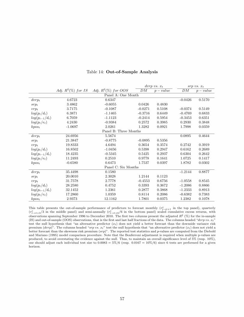
Table 14: Out-of-Sample Analysis

dvrp vs. xt srp vs. xtAdj. R2(%) for IS Adj. R2(%) for OOS DM p− value DM p− value

Panel A: One Month

dvrpt 4.6723 0.6347 -0.0426 0.5170srpt 3.4862 -0.6055 0.0426 0.4830vrpt 3.7175 -0.1087 -0.0271 0.5108 -0.0374 0.5149log(pt/dt) 6.3871 -1.1465 -0.3716 0.6449 -0.4769 0.6833log(pt−1/dt) 6.7059 -1.1123 -0.2414 0.5954 -0.3453 0.6351log(pt/et) 4.2430 -0.9384 0.2572 0.3985 0.2930 0.3848kpost -1.0697 2.0261 1.3282 0.0921 1.7998 0.0359

Panel B: Three Months

dvrpt 24.6956 5.5674 0.0895 0.4644srpt 21.3847 -0.8775 -0.0895 0.5356vrpt 19.8333 4.6494 0.3654 0.3574 0.2742 0.3919log(pt/dt) 16.8502 -1.0456 0.5398 0.2947 0.6162 0.2689log(pt−1/dt) 18.4235 -0.5345 0.5425 0.2937 0.6304 0.2642log(pt/et) 11.2493 0.2510 0.9778 0.1641 1.0725 0.1417kpost -0.6580 0.6473 1.7537 0.0397 1.8782 0.0302

Panel C: Six Months

dvrpt 35.4498 0.1580 -1.2144 0.8877srpt 20.0010 2.3028 1.2144 0.1123vrpt 31.7578 2.7778 -0.4553 0.6756 -1.0558 0.8545log(pt/dt) 28.2580 0.4752 0.3393 0.3672 -1.2086 0.8866log(pt−1/dt) 32.1452 1.2361 0.2877 0.3868 -1.2333 0.8913log(pt/et) 17.2860 1.0359 0.8114 0.2086 -0.6382 0.7383kpost 2.9373 12.1162 1.7801 0.0375 1.2382 0.1078

This table presents the out-of-sample performance of predictors to forecast monthly (ret→t+1 in the top panel), quarterly(ret→t+3/3 in the middle panel) and semi-annually (ret→t+6/6 in the bottom panel) scaled cumulative excess returns, with

observations spanning September 1996 to December 2010. The first two columns present the adjusted R2 (%) for the in-sample(IS) and out-of-sample (OOS) observations, that is the first and last half fractions of the data. The columns headed “dvrp vs. xt”test the null hypothesis that “an alternative predictor (xt) does not yield a better forecast than the downside variance riskpremium (dvrp)”. The columns headed “srp vs. xt” test the null hypothesis that “an alternative predictor (xt) does not yield abetter forecast than the skewness risk premium (srp)”. The reported test statistics and p-values are computed from the Dieboldand Mariano (1995) model comparison procedure. Note that the Bonferroni adjustment is required when multiple p-values areproduced, to avoid overstating the evidence against the null. Thus, to maintain an overall significance level of 5% (resp. 10%),one should adjust each individual test size to 0.0083 = 5%/6 (resp. 0.0167 = 10%/6) since 6 tests are performed for a givenhorizon.

57

Figure 1: S&P 500 Put and Call Contracts per Day

1996 1998 2000 2002 2004 2006 2008 20100

100

200

300

400

500

600

AllCallPut

This graph show the number of outstanding put and call contracts written on the S&P 500 index per day for the 1996-2010period. In addition, it plots the sum of put and call contract numbers. Source: OptionMetrics Ivy DB accessed via WRDS.

58

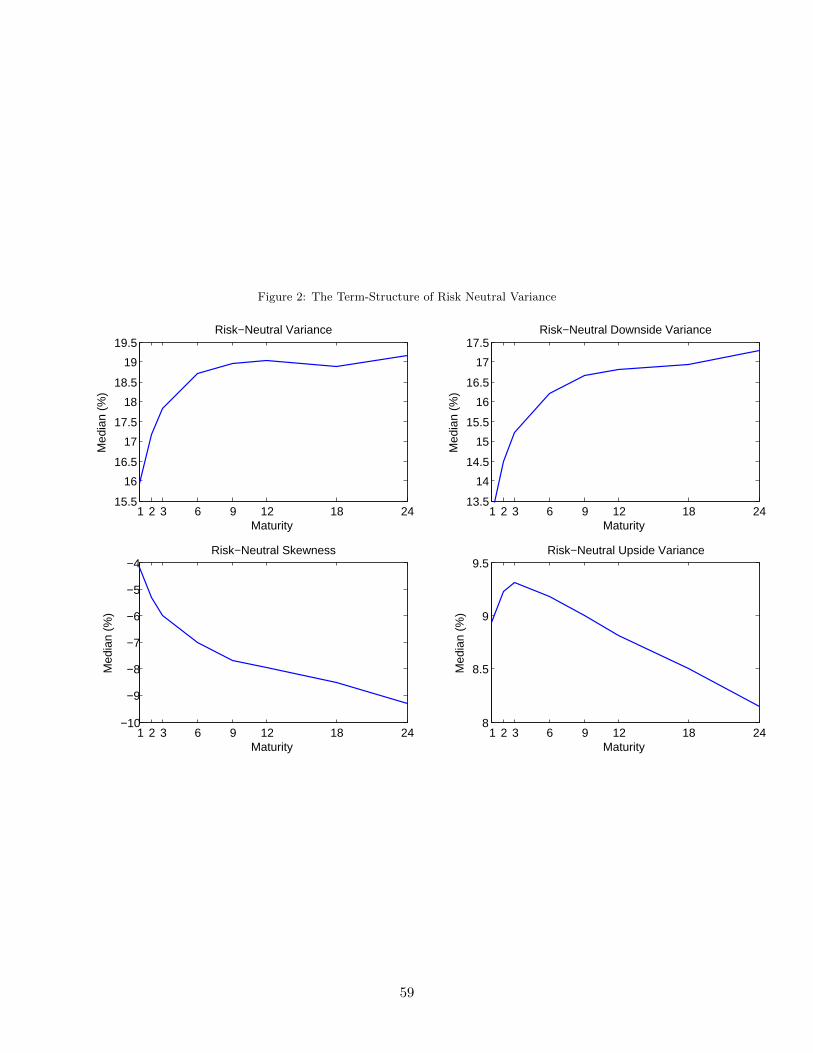
Figure 2: The Term-Structure of Risk Neutral Variance

1 2 3 6 9 12 18 2415.5

16

16.5

17

17.5

18

18.5

19

19.5

Maturity

Med

ian

(%)

Risk−Neutral Variance

1 2 3 6 9 12 18 2413.5

14

14.5

15

15.5

16

16.5

17

17.5

Maturity

Med

ian

(%)

Risk−Neutral Downside Variance

1 2 3 6 9 12 18 24−10

−9

−8

−7

−6

−5

−4

Maturity

Med

ian

(%)

Risk−Neutral Skewness

1 2 3 6 9 12 18 248

8.5

9

9.5

Maturity

Med

ian

(%)

Risk−Neutral Upside Variance

59

Figure 3: The Term-Structure of Realized Variance

1 2 3 6 9 12 18 2416

16.5

17

17.5

18

18.5

19

19.5

Maturity

Med

ian

(%)

Realized Variance

1 2 3 6 9 12 18 2411.5

12

12.5

13

13.5

14

14.5

Maturity

Med

ian

(%)

Realized Downside Variance

1 2 3 6 9 12 18 240.08

0.1

0.12

0.14

0.16

Maturity

Med

ian

(%)

Realized Skewness

1 2 3 6 9 12 18 2411.5

12

12.5

13

13.5

14

14.5

Maturity

Med

ian

(%)

Realized Upside Variance

60

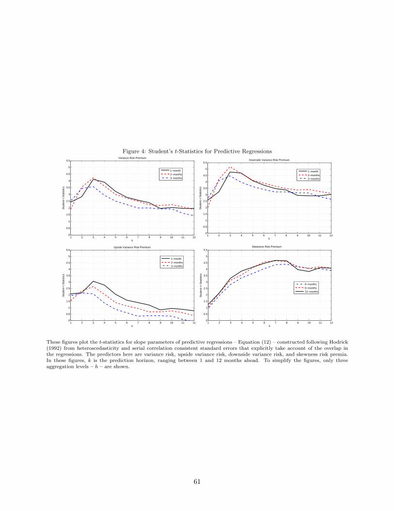
Figure 4: Student’s t-Statistics for Predictive Regressions

1 2 3 4 5 6 7 8 9 10 11 120

0.5

1

1.5

2

2.5

3

3.5

4

4.5

5

5.5

k

Stu

dent

−t S

tatis

tics

Variance Risk Premium

1−month2−months3−months

1 2 3 4 5 6 7 8 9 10 11 120

0.5

1

1.5

2

2.5

3

3.5

4

4.5

5

5.5

k

Stu

dent

−t S

tatis

tics

Downside Variance Risk Premium

1−month2−months3−months

1 2 3 4 5 6 7 8 9 10 11 120

0.5

1

1.5

2

2.5

3

3.5

4

4.5

5

5.5Upside Variance Risk Premium

k

Stu

dent

−t S

tatis

tics

1−month2−months3−months

1 2 3 4 5 6 7 8 9 10 11 120

0.5

1

1.5

2

2.5

3

3.5

4

4.5

5

5.5Skewness Risk Premium

Stu

dent

−t−

Sta

tistic

s

k

6−months9−months12−months

These figures plot the t-statistics for slope parameters of predictive regressions – Equation (12) – constructed following Hodrick(1992) from heteroscedasticity and serial correlation consistent standard errors that explicitly take account of the overlap inthe regressions. The predictors here are variance risk, upside variance risk, downside variance risk, and skewness risk premia.In these figures, k is the prediction horizon, ranging between 1 and 12 months ahead. To simplify the figures, only threeaggregation levels – h – are shown.

61

Figure 5: Adjusted R2 for Predictive Regressions

1 2 3 4 5 6 7 8 9 10 11 120

2

4

6

8

10

12

14

k

Adj

uste

d R

2

Variance Risk Premium

1−month2−months3−months

1 2 3 4 5 6 7 8 9 10 11 120

2

4

6

8

10

12

14

k

Adj

uste

d R

2

Downside Variance Risk Premium

1−month2−months3−months

1 2 3 4 5 6 7 8 9 10 11 120

2

4

6

8

10

12

14

k

Adj

uste

d R

2

Upside Variance Risk Premium

1−month2−months3−months

1 2 3 4 5 6 7 8 9 10 11 120

2

4

6

8

10

12

14

k

Adj

uste

d R

2

Skewness Risk Premium

6−months9−months12−months

These figures plot the adjusted R2s of predictive regressions – Equation (12). The predictors here are variance risk, upsidevariance risk, downside variance risk, and skewness risk premia. In these figures, k is the prediction horizon, ranging between1 and 12 months ahead. To simplify the figures, only three aggregation levels – h – are shown.

62

Figure 6: Comparison of Adjusted R2s for Risk-Neutral and Physical Variance Measures

1 2 3 4 5 6 7 8 9 10 11 12−1

0

1

2

3

4

5

6

7

8

9Risk−Neutral Variance

k

%

6−months9−months12−months

1 2 3 4 5 6 7 8 9 10 11 12

0

1

2

3

4

5

6

7

8

9Realized Variance

k

%

6−months9−months12−months

1 2 3 4 5 6 7 8 9 10 11 12−1

0

1

2

3

4

5

6

7

8

9Risk−Neutral Downside Variance

k

%

1 2 3 4 5 6 7 8 9 10 11 12

0

1

2

3

4

5

6

7

8

9Realized Downside Variance

%

k

1 2 3 4 5 6 7 8 9 10 11 12−1

0

1

2

3

4

5

6

7

8

9

k

%

Risk−Neutral Upside Variance

1 2 3 4 5 6 7 8 9 10 11 12

0

1

2

3

4

5

6

7

8

9

k

%

Realized Upside Variance

1 2 3 4 5 6 7 8 9 10 11 120

1

2

3

4

5

6

7

8

9

k

%

Risk−Neutral Skewness

1 2 3 4 5 6 7 8 9 10 11 12−1

0

1

2

3

4

5

6

7

8

9

k

%

Realized Skewness

These figures plot the adjusted R2s for predictive regressions – Equation (12). The predictors here are risk-neutral and realizedvariance, upside variance, downside variance, and skewness. In these figures, k is the prediction horizon, ranging between 1 and12 months ahead. To simplify the figures, only three aggregation levels – h – are shown.

63

Figure 7: Time-Series for Variance and Skewness Risk Premia

These figures plot the paths of annualized monthly values (×103) for the variance risk premium, upside variance risk premium,downside variance risk premium, and skewness risk premium, extracted from U.S. financial markets data for September 1996to December 2011. The shaded areas represent NBER recessions.

64