dpiw – surface water models rubicon river catchment
TRANSCRIPT
DPIW – SURFACE WATER MODELS
RUBICON RIVER CATCHMENT
Rubicon River Surface Water Model Hydro Tasmania Version No: 2.0
i
DOCUMENT INFORMATION
JOB/PROJECT TITLE Tascatch Variation 2 -Surface Water Models
CLIENT ORGANISATION Department of Primary Industries and Water
CLIENT CONTACT Bryce Graham
DOCUMENT ID NUMBER WR 2007/066
JOB/PROJECT MANAGER Mark Willis
JOB/PROJECT NUMBER E202869/P205357
Document History and Status
Revision Prepared
by
Reviewed
by
Approved
by
Date
approved
Revision
type
1.0 J Bennett M. Willis C. Smythe Dec 2007 FINAL
2.0 J. Bennett M. Willis C. Smythe April 2008 FINAL
Current Document Approval
PREPARED BY James Bennett
Water Resources Mngt Sign Date
REVIEWED BY Mark Willis
Water Resources Mngt Sign Date
APPROVED FOR
SUBMISSION
Crispin Smythe
Water Resources Mngt Sign Date
Current Document Distribution List
Organisation Date Issued To
DPIW April 2008 Bryce Graham
The concepts and information contained in this document are the property of Hydro Tasmania.
This document may only be used for the purposes of assessing our offer of services and for inclusion in
documentation for the engagement of Hydro Tasmania. Use or copying of this document in whole or in part for any
other purpose without the written permission of Hydro Tasmania constitutes an infringement of copyright.
Rubicon River Surface Water Model Hydro Tasmania Version No: 2.0
ii
EXECUTIVE SUMMARY
This report is part of a series of reports which present the methodologies and results
from the development and calibration of surface water hydrological models for 25
catchments (Tascatch – Variation 2) under both current and natural flow conditions. This
report describes the results of the hydrological model developed for the Rubicon River
catchment.
A model was developed for the Rubicon River catchment that facilitates the modelling of
flow data for three scenarios:
• Scenario 1 – No entitlements (Natural Flow);
• Scenario 2 – with Entitlements (with water entitlements extracted);
• Scenario 3 - Environmental Flows and Entitlements (Water entitlements
extracted, however low priority entitlements are limited by an environmental
flow threshold).
The results from the scenario modelling allow the calculation of indices of hydrological
disturbance. These indices include:
• Index of Mean Annual Flow
• Index of Flow Duration Curve Difference
• Index of Seasonal Amplitude
• Index of Seasonal Periodicity
• Hydrological Disturbance Index
The indices were calculated using the formulas stated in the Natural Resource
Management (NRM) Monitoring and Evaluation Framework developed by SKM for the
Murray-Darling Basin (MDBC 08/04).
A user interface is also provided that allows the user to run the model under varying
catchment demand scenarios. This allows the user to add further extractions to
catchments and see what effect these additional extractions have on the available water
in the catchment of concern. The interface provides sub-catchment summary of flow
statistics, duration curves, hydrological indices and water entitlements data. For
information on the use of the user interface refer to the Operating Manual for the NAP
Region Hydrological Models (Hydro Tasmania 2004).

Rubicon River Surface Water Model Hydro Tasmania Version No: 2.0
iii
CONTENTS
EXECUTIVE SUMMARY ii
1. INTRODUCTION 1
2. CATCHMENT CHARACTERISTICS 2
3. DATA COMPILATION 4
3.1 Climate data (Rainfall & Evaporation) 4
3.2 Advantages of using climate DRILL data 4
3.3 Transposition of climate DRILL data to local catchment 5
3.4 Comparison of Data Drill rainfall and site gauges 7
3.5 Streamflow data 8
3.6 Irrigation and water usage 9
3.6.1 Estimation of unlicensed (small) farm dams 16
3.7 Environmental flows 17
4. MODEL DEVELOPMENT 20
4.1 Sub-catchment delineation 20
4.2 Hydstra Model 20
4.3 AWBM Model 22
4.3.1 Channel Routing 24
4.4 Model Calibration 25
4.4.1 Factors affecting the reliability of the model calibration. 32
4.4.2 Model Accuracy - Model Fit Statistics 33
4.4.3 Model accuracy across the catchment 36
5. MODEL RESULTS 39
5.1.1 Indices of hydrological disturbance 39
6. FLOOD FREQUENCY ANALYSIS 42
7. REFERENCES 44
7.1 Personal Communications 45
8. GLOSSARY 46
APPENDIX A 48
Rubicon River Surface Water Model Hydro Tasmania Version No: 2.0
iv
LIST OF FIGURES
Figure 2-1 Sub-catchment boundaries 3
Figure 3-1 Climate Drill Site Locations 6
Figure 3-2 Rainfall and Data Drill Comparisons 8
Figure 3-3 WIMS Water Allocations 15
Figure 4-1 Hydstra Model Schematic 21
Figure 4-2 Two Tap Australian Water Balance Model Schematic 24
Figure 4-3 Monthly Variation of CapAve Parameter 28
Figure 4-4 Daily time series comparison (ML/d) – Rubicon River - Good fit. 29
Figure 4-5 Daily time series comparison (ML/d) – Rubicon River – Good fit. 29
Figure 4-6 Daily time series comparison (ML/d) – Rubicon River – Good fit. 30
Figure 4-7 Monthly time series comparison – volume (ML) 30
Figure 4-8 Long term average monthly, seasonal and annual comparison plot 31
Figure 4-9 Duration Curve – Daily flow percentage difference 35
Figure 4-10 Duration Curve – Monthly volume percentage difference 35
Figure 4-11 Time Series of Monthly Volumes- Site 17201 37
Figure 4-12 Time Series of Monthly Volumes- SubC1_c 38
Figure 5-1 Daily Duration Curve 39
Figure 6-1 Modelled and Observed Flood Frequency Plot – Rubicon at Tidal Limit 43
Figure A-1 Forth catchment – monthly volumes at secondary site. 50
Figure A-2 George catchment – monthly volumes at secondary site. 50
Figure A-3 Leven catchment – monthly volumes at secondary site. 51
Figure A-4 Swan catchment – monthly volumes at secondary site. 51
Figure A-5 Montagu catchment – monthly volumes at secondary site. 52
Rubicon River Surface Water Model Hydro Tasmania Version No: 2.0
v
LIST OF TABLES
Table 3.1 Data Drill Site Locations 7
Table 3.2 Potential calibration sites 9
Table 3.3 Assumed Surety of Unassigned Records 10
Table 3.4 Sub Catchment High and Low Priority Entitlements 11
Table 3.5 Average capacity for dams less than 20 ML by Neal et al (2002) 17
Table 3.6 Environmental Flows 18
Table 4.1 Boughton & Chiew, AWBM surface storage parameters 22
Table 4.2 Hydstra/TSM Modelling Parameter Bounds 25
Table 4.3 Adopted Calibration Parameters 27
Table 4.4 Long term average monthly, seasonal and annual comparisons 31
Table 4.5 Model Fit Statistics 33
Table 4.6 R2 Fit Description 34
Table 5.1 Hydrological Disturbance Indices 40
Table A-1 Model performance at secondary sites 53
Rubicon River Surface Water Model Hydro Tasmania Version No: 2.0
1
1. INTRODUCTION
This report forms part of a larger project commissioned by the Department of Primary
Industries and Water (DPIW) to provide hydrological models for 25 regional catchments
(Tascatch – Variation 2).
The main objectives for the individual catchments are:
• To compile relevant data required for the development and calibration of the hydrological model (Australian Water Balance Model, AWBM) for the Rubicon River catchment;
• To source over 100 years of daily time-step rainfall and streamflow data for input to the hydrologic model;
• To develop and calibrate each hydrologic model, to allow running of the model under varying catchment demand scenarios;
• To develop a User Interface for running the model under these various catchment demand scenarios;
• Prepare a report summarising the methodology adopted, assumptions made, results of calibration and validation and description relating to the use of the developed hydrologic model and associated software.
Rubicon River Surface Water Model Hydro Tasmania Version No: 2.0
2
2. CATCHMENT CHARACTERISTICS
The Rubicon catchment is located in central North Tasmania and discharges into the bay
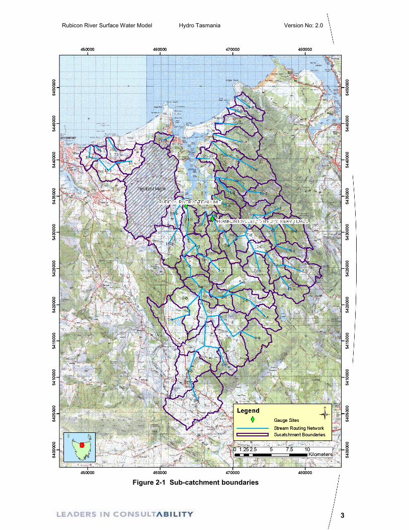
of Port Sorell. The Rubicon River has a catchment area of 263.2 km2, however the
Rubicon surface model covers a much larger area – 572.4 km2 - as it also simulates flow
in smaller catchments that adjoin (but do not flow into) the Rubicon (Figure 2-1). To
differentiate between the Rubicon river catchment area and the entire catchment area of
the model, the former will be called the ‘Rubicon catchment’ and the latter the ‘model
catchment’ henceforth. The larger streams (other than the Rubicon) covered by in the
model catchment area are Pardoe Creek, which discharges into Bass Strait, and Franklin
Rivulet, Branchs Creek and Browns Creek, which discharge into Port Sorrell. The
Panatana River (north-west of the Rubicon) is not accounted for in this model as a DPIW
surface water model of this catchment already exists (see Willis and Peterson 2007).
The headwaters of the Rubicon catchment start in the small, forested hills that rise to 500
m ASL in the south-east of the catchment. The eastern half of the model catchment area
is forested with both natural and plantation forests, while the western half of the model
catchment is mainly used for cropping and other agriculture. The Rubicon catchment is
unusual in that both the upper and lower parts of the catchment are heavily exploited for
agriculture, while the middle of the catchment is forested. (It is more usual that only the
lower part of a catchment, where streamflows are higher and richer alluvial soils occur, is
suitable for farming.) Large volumes of water are extracted from the Rubicon and
surrounding creeks for agriculture and these water extractions can result in significant
localised reductions in streamflow.
The model catchment is dry relative to many Tasmanian catchments, receiving 700 mm
in the north-east to 1000 mm in the hills in the South (Figure 2-1).
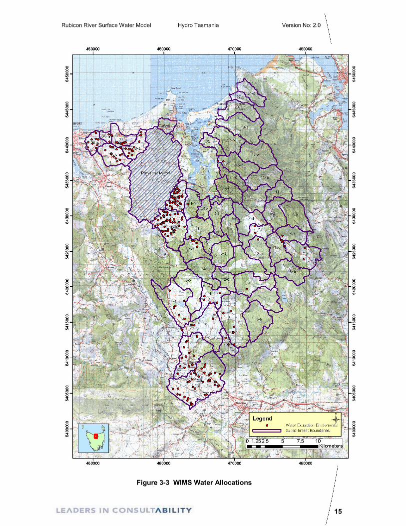
There are 291 registered (current) entitlements for water extraction registered on the
Water Information Management System (WIMS July 2007). Most of these extractions
are concentrated in only a few sub-catchments (Figure 3-3). Licenced extractions relate
mainly to agriculture. The largest extraction entitlement is 1860 ML for a large irrigation
dam in the South of the Rubicon Catchment.
For modelling purposes, the Rubicon River catchment was divided into 53 sub areas.
The delineation of these areas and the assumed stream routing network is shown in
Figure 2-1.
Rubicon River Surface Water Model Hydro Tasmania Version No: 2.0
3
Figure 2-1 Sub-catchment boundaries
Rubicon River Surface Water Model Hydro Tasmania Version No: 2.0
4
3. DATA COMPILATION
3.1 Climate data (Rainfall & Evaporation)
Daily time-step climate data was obtained from the Queensland Department of Natural
Resources & Mines (QDNRM).
The Department provides time series climate drill data from 0.05o x 0.05o (about 5 km x 5
km) interpolated gridded rainfall and evaporation data based on over 6000 rainfall and
evaporation stations in Australia (see www.nrm.qld.gov.au/silo) for further details of climate
drill data.
3.2 Advantages of using climate DRILL data
This data has a number of benefits over other sources of rainfall data including:
• Continuous data back to 1889 (however, further back there are less input sites
available and therefore quality is reduced. The makers of the data set state that
gauge numbers have been somewhat static since 1957, therefore back to 1957
distribution is considered “good” but prior to 1957 site availability may need to be
checked in the study area).
• Evaporation data (along with a number of other climatic variables) is also
included which can be used for the AWBM model. According to the QDNRM web
site, all Data Drill evaporation information combines a mixture of the following
data:
1. Observed data from the Commonwealth Bureau of Meteorology (BoM);
2. Interpolated daily climate surfaces from the on-line NR&M climate archive;
3. Observed pre-1957 climate data from the CLIMARC project (LWRRDC QPI-
43). NR&M was a major research collaborator on the CLIMARC project, and
these data have been integrated into the on-line NR&M climate archive;
4. Interpolated pre-1957 climate surfaces. This data set, derived mainly from the
CLIMARC project data, is available in the on-line NR&M climate archive;
5. Incorporation of Automatic Weather Station (AWS) data records. Typically, an
AWS is placed at a user's site to provide accurate local weather
measurements.
For the Rubicon model the evaporation data was examined and it was found that prior to
Rubicon River Surface Water Model Hydro Tasmania Version No: 2.0
5
1970 the evaporation information is based on the long term daily averages of the post
1970 data. In the absence of any reliable long term site data this is considered to be the
best available evaporation data set for this catchment.
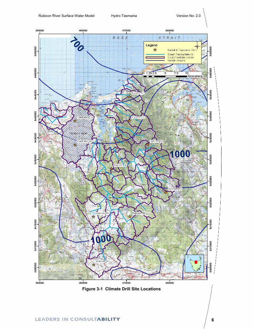
3.3 Transposition of climate DRILL data to local catchment
Ten climate Data Drill sites were selected to give good coverage of the model catchment.
Two of these sites correspond to the same location as Data Drill information sourced for
the Panatana River catchment model and another corresponds to the same location as a
site used in the Meander, Quamby and Liffey catchment model.
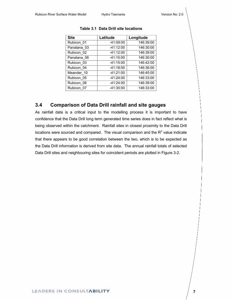
See the following Figure 3-1 for a map of the climate Data Drill sites and Table 3.1 for the
location information.
Rubicon River Surface Water Model Hydro Tasmania Version No: 2.0
6
Figure 3-1 Climate Drill Site Locations
Rubicon River Surface Water Model Hydro Tasmania Version No: 2.0
7
Table 3.1 Data Drill site locations
Site Latitude Longitude
Rubicon_01 -41:09:00 146:39:00
Panatana_03 -41:12:00 146:30:00
Rubicon_02 -41:12:00 146:39:00
Panatana_06 -41:15:00 146:30:00
Rubicon_03 -41:15:00 146:42:00
Rubicon_04 -41:18:00 146:36:00
Meander_10 -41:21:00 146:45:00
Rubicon_05 -41:24:00 146:33:00
Rubicon_06 -41:24:00 146:39:00
Rubicon_07 -41:30:00 146:33:00
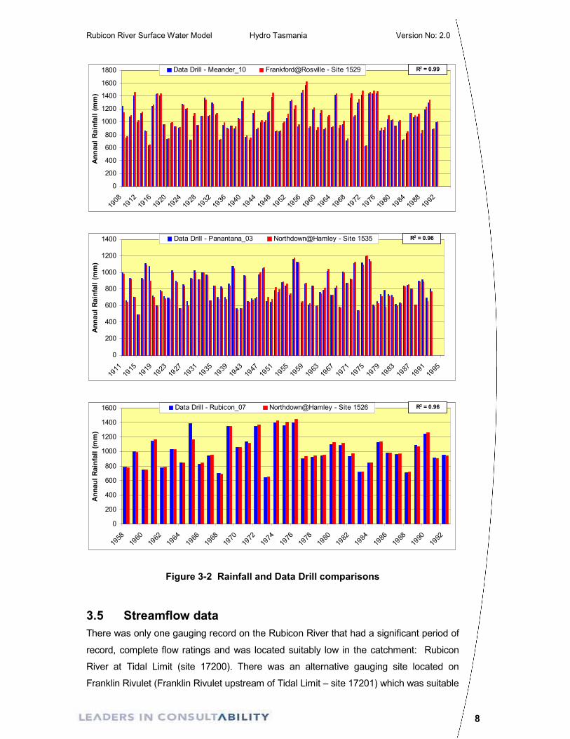
3.4 Comparison of Data Drill rainfall and site gauges
As rainfall data is a critical input to the modelling process it is important to have
confidence that the Data Drill long term generated time series does in fact reflect what is
being observed within the catchment. Rainfall sites in closest proximity to the Data Drill
locations were sourced and compared. The visual comparison and the R2 value indicate
that there appears to be good correlation between the two, which is to be expected as
the Data Drill information is derived from site data. The annual rainfall totals of selected
Data Drill sites and neighbouring sites for coincident periods are plotted in Figure 3-2.
Rubicon River Surface Water Model Hydro Tasmania Version No: 2.0
8
0
200
400
600
800
1000
1200
1400
1600
1800
1908
1912
1916
1920
1924
1928
1932
1936
1940
1944
1948
1952
1956
1960
1964
1968
1972
1976
1980
1984
1988
1992
Annaul R
ain
fall (m
m)
Data Drill - Meander_10 Frankford@Rosville - Site 1529 R2 = 0.99
0
200
400
600
800
1000
1200
1400
1911
1915
1919
1923
1927
1931
1935
1939
1943
1947
1951
1955
1959
1963
1967
1971
1975
1979
1983
1987
1991
1995
Annaul R
ain
fall (m
m)
Data Drill - Panantana_03 Northdown@Hamley - Site 1535 R2 = 0.96
0
200
400
600
800
1000
1200
1400
1600
1958
1960
1962
1964
1966
1968
1970
1972
1974
1976
1978
1980
1982
1984
1986
1988
1990
1992
Annaul R
ain
fall (m
m)
Data Drill - Rubicon_07 Northdown@Hamley - Site 1526 R2 = 0.96
Figure 3-2 Rainfall and Data Drill comparisons
3.5 Streamflow data
There was only one gauging record on the Rubicon River that had a significant period of
record, complete flow ratings and was located suitably low in the catchment: Rubicon
River at Tidal Limit (site 17200). There was an alternative gauging site located on
Franklin Rivulet (Franklin Rivulet upstream of Tidal Limit – site 17201) which was suitable

Rubicon River Surface Water Model Hydro Tasmania Version No: 2.0
9
as a comparison site to validate the model. The details of these sites are given in the
following table.
Table 3.2 Potential calibration sites
Site Name Site No.
Sub-catchment Location
Period of Record Easting Northing Comments
Rubicon River at Tidal Limit
17200 SC1_h 22/06/1967–Present 463580 5433600 Low in catchment, good record
Franklin Rivulet upstream of Tidal Limit
17201 SC7_f 01/01/1975 – 10/02/1994
467200 5431800 Smaller stream in model catchment
A continuous time series in ML/day was provided at the calibration site by DPIW and it is
therefore assumed that this represents the best available flow record. Hence no detailed
review or alteration of this data has been undertaken.
Investigations of the rating histories and qualities contained on the Hydro Tasmania’s
archives indicate that the record for Rubicon at Tidal Limit is based on a weir control
structure with 5 ratings covering the whole period of record and the data appears to be
reliable during the period of interest.
3.6 Irrigation and water usage
Information on the current water entitlement allocations in the catchment was obtained
from DPIW and is sourced from the Water Information Management System (WIMS July
2007). The WIMS extractions or licenses in the catchment are of a given Surety (from 1
to 8), with Surety 1-3 representing high priority extractions for modelling purposes and
Surety 4-8 representing the lowest priority. The data provided by DPIW contained a
number of sites which had a Surety of 0. DPIW staff advised that in these cases the
Surety should be determined by the extraction “Purpose” and assigned as follows:
Rubicon River Surface Water Model Hydro Tasmania Version No: 2.0
10
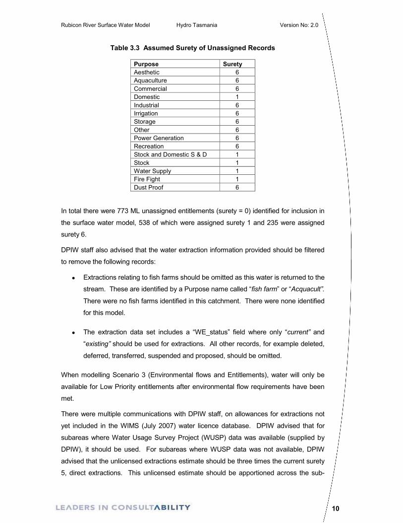
Table 3.3 Assumed Surety of Unassigned Records
Purpose Surety
Aesthetic 6
Aquaculture 6
Commercial 6
Domestic 1
Industrial 6
Irrigation 6
Storage 6
Other 6
Power Generation 6
Recreation 6
Stock and Domestic S & D 1
Stock 1
Water Supply 1
Fire Fight 1
Dust Proof 6
In total there were 773 ML unassigned entitlements (surety = 0) identified for inclusion in
the surface water model, 538 of which were assigned surety 1 and 235 were assigned
surety 6.
DPIW staff also advised that the water extraction information provided should be filtered
to remove the following records:
• Extractions relating to fish farms should be omitted as this water is returned to the
stream. These are identified by a Purpose name called “fish farm” or “Acquacult”.
There were no fish farms identified in this catchment. There were none identified
for this model.
• The extraction data set includes a “WE_status” field where only “current” and
“existing” should be used for extractions. All other records, for example deleted,
deferred, transferred, suspended and proposed, should be omitted.
When modelling Scenario 3 (Environmental flows and Entitlements), water will only be
available for Low Priority entitlements after environmental flow requirements have been
met.
There were multiple communications with DPIW staff, on allowances for extractions not
yet included in the WIMS (July 2007) water licence database. DPIW advised that for
subareas where Water Usage Survey Project (WUSP) data was available (supplied by
DPIW), it should be used. For subareas where WUSP data was not available, DPIW
advised that the unlicensed extractions estimate should be three times the current surety
5, direct extractions. This unlicensed estimate should be apportioned across the sub-
Rubicon River Surface Water Model Hydro Tasmania Version No: 2.0
11
catchments the same as the surety 5 extractions.
WUSP data was available for 1 subcatchment in the model: SC1_a. According to WUSP
SC1_a has 881 ML unlicenced extraction per year. For the remaining 52
subcatchments, there were 679 ML of direct surety 5 extractions (current) in the WIMS
database and accordingly an estimate of 2037 ML of unlicensed extractions was
apportioned across the catchment. In total there were 2918 ML unlicenced extractions
across all subcatchments. DPIW advised that these unlicensed extractions should be
assigned as surety 6 and be extracted during the months of October through to April.
In addition to the extractions detailed above, an estimate was a made for small farm dam
extractions currently not requiring a permit and hence not listed in the WIMS database.
Theses extractions are referred to in this report as unlicensed (small) farm dam
extractions and details of the extraction estimate is covered in Section 3.6.1.
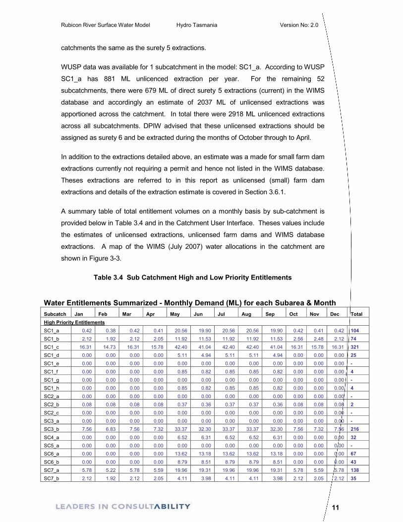
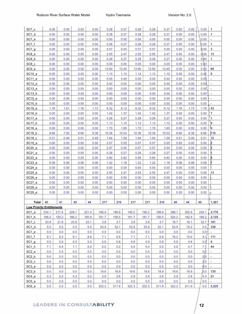
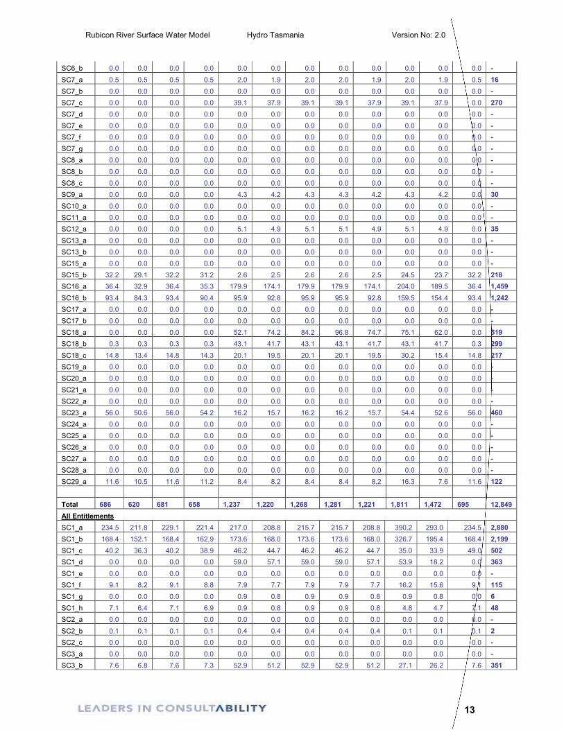
A summary table of total entitlement volumes on a monthly basis by sub-catchment is
provided below in Table 3.4 and in the Catchment User Interface. Theses values include
the estimates of unlicensed extractions, unlicensed farm dams and WIMS database
extractions. A map of the WIMS (July 2007) water allocations in the catchment are
shown in Figure 3-3.
Table 3.4 Sub Catchment High and Low Priority Entitlements
Water Entitlements Summarized - Monthly Demand (ML) for each Subarea & Month
Subcatch Jan Feb Mar Apr May Jun Jul Aug Sep Oct Nov Dec Total
High Priority Entitlements
SC1_a 0.42 0.38 0.42 0.41 20.56 19.90 20.56 20.56 19.90 0.42 0.41 0.42 104
SC1_b 2.12 1.92 2.12 2.05 11.92 11.53 11.92 11.92 11.53 2.56 2.48 2.12 74
SC1_c 16.31 14.73 16.31 15.78 42.40 41.04 42.40 42.40 41.04 16.31 15.78 16.31 321
SC1_d 0.00 0.00 0.00 0.00 5.11 4.94 5.11 5.11 4.94 0.00 0.00 0.00 25
SC1_e 0.00 0.00 0.00 0.00 0.00 0.00 0.00 0.00 0.00 0.00 0.00 0.00 -
SC1_f 0.00 0.00 0.00 0.00 0.85 0.82 0.85 0.85 0.82 0.00 0.00 0.00 4
SC1_g 0.00 0.00 0.00 0.00 0.00 0.00 0.00 0.00 0.00 0.00 0.00 0.00 -
SC1_h 0.00 0.00 0.00 0.00 0.85 0.82 0.85 0.85 0.82 0.00 0.00 0.00 4
SC2_a 0.00 0.00 0.00 0.00 0.00 0.00 0.00 0.00 0.00 0.00 0.00 0.00 -
SC2_b 0.08 0.08 0.08 0.08 0.37 0.36 0.37 0.37 0.36 0.08 0.08 0.08 2
SC2_c 0.00 0.00 0.00 0.00 0.00 0.00 0.00 0.00 0.00 0.00 0.00 0.00 -
SC3_a 0.00 0.00 0.00 0.00 0.00 0.00 0.00 0.00 0.00 0.00 0.00 0.00 -
SC3_b 7.56 6.83 7.56 7.32 33.37 32.30 33.37 33.37 32.30 7.56 7.32 7.56 216
SC4_a 0.00 0.00 0.00 0.00 6.52 6.31 6.52 6.52 6.31 0.00 0.00 0.00 32
SC5_a 0.00 0.00 0.00 0.00 0.00 0.00 0.00 0.00 0.00 0.00 0.00 0.00 -
SC6_a 0.00 0.00 0.00 0.00 13.62 13.18 13.62 13.62 13.18 0.00 0.00 0.00 67
SC6_b 0.00 0.00 0.00 0.00 8.79 8.51 8.79 8.79 8.51 0.00 0.00 0.00 43
SC7_a 5.78 5.22 5.78 5.59 19.96 19.31 19.96 19.96 19.31 5.78 5.59 5.78 138
SC7_b 2.12 1.92 2.12 2.05 4.11 3.98 4.11 4.11 3.98 2.12 2.05 2.12 35
Rubicon River Surface Water Model Hydro Tasmania Version No: 2.0
12
SC7_c 0.00 0.00 0.00 0.00 0.28 0.27 0.28 0.28 0.27 0.00 0.00 0.00 1
SC7_d 0.00 0.00 0.00 0.00 0.28 0.27 0.28 0.28 0.27 0.00 0.00 0.00 1
SC7_e 0.00 0.00 0.00 0.00 0.00 0.00 0.00 0.00 0.00 0.00 0.00 0.00 -
SC7_f 0.00 0.00 0.00 0.00 0.28 0.27 0.28 0.28 0.27 0.00 0.00 0.00 1
SC7_g 0.00 0.00 0.00 0.00 0.57 0.55 0.57 0.57 0.55 0.00 0.00 0.00 3
SC8_a 0.00 0.00 0.00 0.00 2.55 2.47 2.55 2.55 2.47 0.00 0.00 0.00 13
SC8_b 0.00 0.00 0.00 0.00 0.28 0.27 0.28 0.28 0.27 0.00 0.00 0.00 1
SC8_c 0.00 0.00 0.00 0.00 0.00 0.00 0.00 0.00 0.00 0.00 0.00 0.00 -
SC9_a 0.00 0.00 0.00 0.00 13.90 13.45 13.90 13.90 13.45 0.00 0.00 0.00 69
SC10_a 0.00 0.00 0.00 0.00 1.13 1.10 1.13 1.13 1.10 0.00 0.00 0.00 6
SC11_a 0.00 0.00 0.00 0.00 0.00 0.00 0.00 0.00 0.00 0.00 0.00 0.00 -
SC12_a 0.00 0.00 0.00 0.00 0.00 0.00 0.00 0.00 0.00 0.00 0.00 0.00 -
SC13_a 0.00 0.00 0.00 0.00 0.00 0.00 0.00 0.00 0.00 0.00 0.00 0.00 -
SC13_b 0.00 0.00 0.00 0.00 0.00 0.00 0.00 0.00 0.00 0.00 0.00 0.00 -
SC15_a 0.00 0.00 0.00 0.00 0.00 0.00 0.00 0.00 0.00 0.00 0.00 0.00 -
SC15_b 0.00 0.00 0.00 0.00 0.00 0.00 0.00 0.00 0.00 0.00 0.00 0.00 -
SC16_a 1.78 1.61 1.78 1.73 6.32 6.12 6.32 6.32 6.12 1.78 1.73 1.78 43
SC16_b 0.00 0.00 0.00 0.00 1.42 1.37 1.42 1.42 1.37 0.00 0.00 0.00 7
SC17_a 0.00 0.00 0.00 0.00 0.28 0.27 0.28 0.28 0.27 0.00 0.00 0.00 1
SC17_b 0.00 0.00 0.00 0.00 1.13 1.10 1.13 1.13 1.10 0.00 0.00 0.00 6
SC18_a 0.00 0.00 0.00 0.00 1.70 1.65 1.70 1.70 1.65 0.00 0.00 0.00 8
SC18_b 8.66 7.82 8.66 8.38 10.36 10.03 10.36 10.36 10.03 8.66 8.38 8.66 110
SC18_c 0.51 0.46 0.51 0.49 1.64 1.59 1.64 1.64 1.59 0.51 0.49 0.51 12
SC19_a 0.00 0.00 0.00 0.00 0.57 0.55 0.57 0.57 0.55 0.00 0.00 0.00 3
SC20_a 0.00 0.00 0.00 0.00 0.57 0.55 0.57 0.57 0.55 0.00 0.00 0.00 3
SC21_a 0.00 0.00 0.00 0.00 0.28 0.27 0.28 0.28 0.27 0.00 0.00 0.00 1
SC22_a 0.00 0.00 0.00 0.00 0.85 0.82 0.85 0.85 0.82 0.00 0.00 0.00 4
SC23_a 0.08 0.08 0.08 0.08 1.22 1.18 1.22 1.22 1.18 0.08 0.08 0.08 7
SC24_a 0.00 0.00 0.00 0.00 0.00 0.00 0.00 0.00 0.00 0.00 0.00 0.00 -
SC25_a 0.00 0.00 0.00 0.00 2.55 2.47 2.55 2.55 2.47 0.00 0.00 0.00 13
SC26_a 0.00 0.00 0.00 0.00 0.00 0.00 0.00 0.00 0.00 0.00 0.00 0.00 -
SC27_a 0.00 0.00 0.00 0.00 0.00 0.00 0.00 0.00 0.00 0.00 0.00 0.00 -
SC28_a 0.00 0.00 0.00 0.00 0.00 0.00 0.00 0.00 0.00 0.00 0.00 0.00 -
SC29_a 0.00 0.00 0.00 0.00 0.00 0.00 0.00 0.00 0.00 0.00 0.00 0.00 -
Total 45 41 45 44 217 210 217 217 210 46 44 45 1,381
Low Priority Entitlements
SC1_a 234.1 211.4 228.7 221.0 196.4 188.9 195.2 195.2 188.9 389.7 292.6 234.1 2,776
SC1_b 166.2 150.2 166.2 160.9 161.7 156.5 161.7 161.7 156.5 324.2 192.9 166.2 2,125
SC1_c 23.9 21.6 23.9 23.1 3.8 3.7 3.8 3.8 3.7 18.7 18.1 32.7 181
SC1_d 0.0 0.0 0.0 0.0 53.9 52.1 53.9 53.9 52.1 53.9 18.2 0.0 338
SC1_e 0.0 0.0 0.0 0.0 0.0 0.0 0.0 0.0 0.0 0.0 0.0 0.0 -
SC1_f 9.1 8.2 9.1 8.8 7.1 6.9 7.1 7.1 6.9 16.2 15.6 9.1 111
SC1_g 0.0 0.0 0.0 0.0 0.9 0.8 0.9 0.9 0.8 0.9 0.8 0.0 6
SC1_h 7.1 6.4 7.1 6.9 0.0 0.0 0.0 0.0 0.0 4.8 4.7 7.1 44
SC2_a 0.0 0.0 0.0 0.0 0.0 0.0 0.0 0.0 0.0 0.0 0.0 0.0 -
SC2_b 0.0 0.0 0.0 0.0 0.0 0.0 0.0 0.0 0.0 0.0 0.0 0.0 -
SC2_c 0.0 0.0 0.0 0.0 0.0 0.0 0.0 0.0 0.0 0.0 0.0 0.0 -
SC3_a 0.0 0.0 0.0 0.0 0.0 0.0 0.0 0.0 0.0 0.0 0.0 0.0 -
SC3_b 0.0 0.0 0.0 0.0 19.6 18.9 19.6 19.6 18.9 19.6 18.9 0.0 135
SC4_a 0.3 0.2 0.3 0.2 2.9 2.8 2.9 2.9 2.8 2.9 2.8 0.3 21
SC5_a 0.0 0.0 0.0 0.0 0.0 0.0 0.0 0.0 0.0 0.0 0.0 0.0 -
SC6_a 0.0 0.0 0.0 0.0 322.3 311.9 322.3 322.3 311.9 322.3 311.9 0.0 2,225
Rubicon River Surface Water Model Hydro Tasmania Version No: 2.0
13
SC6_b 0.0 0.0 0.0 0.0 0.0 0.0 0.0 0.0 0.0 0.0 0.0 0.0 -
SC7_a 0.5 0.5 0.5 0.5 2.0 1.9 2.0 2.0 1.9 2.0 1.9 0.5 16
SC7_b 0.0 0.0 0.0 0.0 0.0 0.0 0.0 0.0 0.0 0.0 0.0 0.0 -
SC7_c 0.0 0.0 0.0 0.0 39.1 37.9 39.1 39.1 37.9 39.1 37.9 0.0 270
SC7_d 0.0 0.0 0.0 0.0 0.0 0.0 0.0 0.0 0.0 0.0 0.0 0.0 -
SC7_e 0.0 0.0 0.0 0.0 0.0 0.0 0.0 0.0 0.0 0.0 0.0 0.0 -
SC7_f 0.0 0.0 0.0 0.0 0.0 0.0 0.0 0.0 0.0 0.0 0.0 0.0 -
SC7_g 0.0 0.0 0.0 0.0 0.0 0.0 0.0 0.0 0.0 0.0 0.0 0.0 -
SC8_a 0.0 0.0 0.0 0.0 0.0 0.0 0.0 0.0 0.0 0.0 0.0 0.0 -
SC8_b 0.0 0.0 0.0 0.0 0.0 0.0 0.0 0.0 0.0 0.0 0.0 0.0 -
SC8_c 0.0 0.0 0.0 0.0 0.0 0.0 0.0 0.0 0.0 0.0 0.0 0.0 -
SC9_a 0.0 0.0 0.0 0.0 4.3 4.2 4.3 4.3 4.2 4.3 4.2 0.0 30
SC10_a 0.0 0.0 0.0 0.0 0.0 0.0 0.0 0.0 0.0 0.0 0.0 0.0 -
SC11_a 0.0 0.0 0.0 0.0 0.0 0.0 0.0 0.0 0.0 0.0 0.0 0.0 -
SC12_a 0.0 0.0 0.0 0.0 5.1 4.9 5.1 5.1 4.9 5.1 4.9 0.0 35
SC13_a 0.0 0.0 0.0 0.0 0.0 0.0 0.0 0.0 0.0 0.0 0.0 0.0 -
SC13_b 0.0 0.0 0.0 0.0 0.0 0.0 0.0 0.0 0.0 0.0 0.0 0.0 -
SC15_a 0.0 0.0 0.0 0.0 0.0 0.0 0.0 0.0 0.0 0.0 0.0 0.0 -
SC15_b 32.2 29.1 32.2 31.2 2.6 2.5 2.6 2.6 2.5 24.5 23.7 32.2 218
SC16_a 36.4 32.9 36.4 35.3 179.9 174.1 179.9 179.9 174.1 204.0 189.5 36.4 1,459
SC16_b 93.4 84.3 93.4 90.4 95.9 92.8 95.9 95.9 92.8 159.5 154.4 93.4 1,242
SC17_a 0.0 0.0 0.0 0.0 0.0 0.0 0.0 0.0 0.0 0.0 0.0 0.0 -
SC17_b 0.0 0.0 0.0 0.0 0.0 0.0 0.0 0.0 0.0 0.0 0.0 0.0 -
SC18_a 0.0 0.0 0.0 0.0 52.1 74.2 84.2 96.8 74.7 75.1 62.0 0.0 519
SC18_b 0.3 0.3 0.3 0.3 43.1 41.7 43.1 43.1 41.7 43.1 41.7 0.3 299
SC18_c 14.8 13.4 14.8 14.3 20.1 19.5 20.1 20.1 19.5 30.2 15.4 14.8 217
SC19_a 0.0 0.0 0.0 0.0 0.0 0.0 0.0 0.0 0.0 0.0 0.0 0.0 -
SC20_a 0.0 0.0 0.0 0.0 0.0 0.0 0.0 0.0 0.0 0.0 0.0 0.0 -
SC21_a 0.0 0.0 0.0 0.0 0.0 0.0 0.0 0.0 0.0 0.0 0.0 0.0 -
SC22_a 0.0 0.0 0.0 0.0 0.0 0.0 0.0 0.0 0.0 0.0 0.0 0.0 -
SC23_a 56.0 50.6 56.0 54.2 16.2 15.7 16.2 16.2 15.7 54.4 52.6 56.0 460
SC24_a 0.0 0.0 0.0 0.0 0.0 0.0 0.0 0.0 0.0 0.0 0.0 0.0 -
SC25_a 0.0 0.0 0.0 0.0 0.0 0.0 0.0 0.0 0.0 0.0 0.0 0.0 -
SC26_a 0.0 0.0 0.0 0.0 0.0 0.0 0.0 0.0 0.0 0.0 0.0 0.0 -
SC27_a 0.0 0.0 0.0 0.0 0.0 0.0 0.0 0.0 0.0 0.0 0.0 0.0 -
SC28_a 0.0 0.0 0.0 0.0 0.0 0.0 0.0 0.0 0.0 0.0 0.0 0.0 -
SC29_a 11.6 10.5 11.6 11.2 8.4 8.2 8.4 8.4 8.2 16.3 7.6 11.6 122
Total 686 620 681 658 1,237 1,220 1,268 1,281 1,221 1,811 1,472 695 12,849
All Entitlements
SC1_a 234.5 211.8 229.1 221.4 217.0 208.8 215.7 215.7 208.8 390.2 293.0 234.5 2,880
SC1_b 168.4 152.1 168.4 162.9 173.6 168.0 173.6 173.6 168.0 326.7 195.4 168.4 2,199
SC1_c 40.2 36.3 40.2 38.9 46.2 44.7 46.2 46.2 44.7 35.0 33.9 49.0 502
SC1_d 0.0 0.0 0.0 0.0 59.0 57.1 59.0 59.0 57.1 53.9 18.2 0.0 363
SC1_e 0.0 0.0 0.0 0.0 0.0 0.0 0.0 0.0 0.0 0.0 0.0 0.0 -
SC1_f 9.1 8.2 9.1 8.8 7.9 7.7 7.9 7.9 7.7 16.2 15.6 9.1 115
SC1_g 0.0 0.0 0.0 0.0 0.9 0.8 0.9 0.9 0.8 0.9 0.8 0.0 6
SC1_h 7.1 6.4 7.1 6.9 0.9 0.8 0.9 0.9 0.8 4.8 4.7 7.1 48
SC2_a 0.0 0.0 0.0 0.0 0.0 0.0 0.0 0.0 0.0 0.0 0.0 0.0 -
SC2_b 0.1 0.1 0.1 0.1 0.4 0.4 0.4 0.4 0.4 0.1 0.1 0.1 2
SC2_c 0.0 0.0 0.0 0.0 0.0 0.0 0.0 0.0 0.0 0.0 0.0 0.0 -
SC3_a 0.0 0.0 0.0 0.0 0.0 0.0 0.0 0.0 0.0 0.0 0.0 0.0 -
SC3_b 7.6 6.8 7.6 7.3 52.9 51.2 52.9 52.9 51.2 27.1 26.2 7.6 351

Rubicon River Surface Water Model Hydro Tasmania Version No: 2.0
14
SC4_a 0.3 0.2 0.3 0.2 9.4 9.1 9.4 9.4 9.1 2.9 2.8 0.3 53
SC5_a 0.0 0.0 0.0 0.0 0.0 0.0 0.0 0.0 0.0 0.0 0.0 0.0 -
SC6_a 0.0 0.0 0.0 0.0 335.9 325.1 335.9 335.9 325.1 322.3 311.9 0.0 2,292
SC6_b 0.0 0.0 0.0 0.0 8.8 8.5 8.8 8.8 8.5 0.0 0.0 0.0 43
SC7_a 6.3 5.7 6.3 6.1 21.9 21.2 21.9 21.9 21.2 7.7 7.5 6.3 154
SC7_b 2.1 1.9 2.1 2.1 4.1 4.0 4.1 4.1 4.0 2.1 2.1 2.1 35
SC7_c 0.0 0.0 0.0 0.0 39.4 38.1 39.4 39.4 38.1 39.1 37.9 0.0 271
SC7_d 0.0 0.0 0.0 0.0 0.3 0.3 0.3 0.3 0.3 0.0 0.0 0.0 1
SC7_e 0.0 0.0 0.0 0.0 0.0 0.0 0.0 0.0 0.0 0.0 0.0 0.0 -
SC7_f 0.0 0.0 0.0 0.0 0.3 0.3 0.3 0.3 0.3 0.0 0.0 0.0 1
SC7_g 0.0 0.0 0.0 0.0 0.6 0.5 0.6 0.6 0.5 0.0 0.0 0.0 3
SC8_a 0.0 0.0 0.0 0.0 2.6 2.5 2.6 2.6 2.5 0.0 0.0 0.0 13
SC8_b 0.0 0.0 0.0 0.0 0.3 0.3 0.3 0.3 0.3 0.0 0.0 0.0 1
SC8_c 0.0 0.0 0.0 0.0 0.0 0.0 0.0 0.0 0.0 0.0 0.0 0.0 -
SC9_a 0.0 0.0 0.0 0.0 18.2 17.7 18.2 18.2 17.7 4.3 4.2 0.0 99
SC10_a 0.0 0.0 0.0 0.0 1.1 1.1 1.1 1.1 1.1 0.0 0.0 0.0 6
SC11_a 0.0 0.0 0.0 0.0 0.0 0.0 0.0 0.0 0.0 0.0 0.0 0.0 -
SC12_a 0.0 0.0 0.0 0.0 5.1 4.9 5.1 5.1 4.9 5.1 4.9 0.0 35
SC13_a 0.0 0.0 0.0 0.0 0.0 0.0 0.0 0.0 0.0 0.0 0.0 0.0 -
SC13_b 0.0 0.0 0.0 0.0 0.0 0.0 0.0 0.0 0.0 0.0 0.0 0.0 -
SC15_a 0.0 0.0 0.0 0.0 0.0 0.0 0.0 0.0 0.0 0.0 0.0 0.0 -
SC15_b 32.2 29.1 32.2 31.2 2.6 2.5 2.6 2.6 2.5 24.5 23.7 32.2 218
SC16_a 38.2 34.5 38.2 37.0 186.2 180.2 186.2 186.2 180.2 205.8 191.2 38.2 1,502
SC16_b 93.4 84.3 93.4 90.4 97.3 94.2 97.3 97.3 94.2 159.5 154.4 93.4 1,249
SC17_a 0.0 0.0 0.0 0.0 0.3 0.3 0.3 0.3 0.3 0.0 0.0 0.0 1
SC17_b 0.0 0.0 0.0 0.0 1.1 1.1 1.1 1.1 1.1 0.0 0.0 0.0 6
SC18_a 0.0 0.0 0.0 0.0 53.8 75.9 85.9 98.5 76.3 75.1 62.0 0.0 527
SC18_b 9.0 8.1 9.0 8.7 53.4 51.7 53.4 53.4 51.7 51.7 50.1 9.0 409
SC18_c 15.3 13.8 15.3 14.8 21.8 21.1 21.8 21.8 21.1 30.7 15.9 15.3 229
SC19_a 0.0 0.0 0.0 0.0 0.6 0.5 0.6 0.6 0.5 0.0 0.0 0.0 3
SC20_a 0.0 0.0 0.0 0.0 0.6 0.5 0.6 0.6 0.5 0.0 0.0 0.0 3
SC21_a 0.0 0.0 0.0 0.0 0.3 0.3 0.3 0.3 0.3 0.0 0.0 0.0 1
SC22_a 0.0 0.0 0.0 0.0 0.9 0.8 0.9 0.9 0.8 0.0 0.0 0.0 4
SC23_a 56.1 50.7 56.1 54.3 17.4 16.9 17.4 17.4 16.9 54.5 52.7 56.1 467
SC24_a 0.0 0.0 0.0 0.0 0.0 0.0 0.0 0.0 0.0 0.0 0.0 0.0 -
SC25_a 0.0 0.0 0.0 0.0 2.6 2.5 2.6 2.6 2.5 0.0 0.0 0.0 13
SC26_a 0.0 0.0 0.0 0.0 0.0 0.0 0.0 0.0 0.0 0.0 0.0 0.0 -
SC27_a 0.0 0.0 0.0 0.0 0.0 0.0 0.0 0.0 0.0 0.0 0.0 0.0 -
SC28_a 0.0 0.0 0.0 0.0 0.0 0.0 0.0 0.0 0.0 0.0 0.0 0.0 -
SC29_a 11.6 10.5 11.6 11.2 8.4 8.2 8.4 8.4 8.2 16.3 7.6 11.6 122
Total 731 661 726 702 1,454 1,430 1,485 1,497 1,430 1,857 1,517 740 14,230
Rubicon River Surface Water Model Hydro Tasmania Version No: 2.0
15
Figure 3-3 WIMS Water Allocations

Rubicon River Surface Water Model Hydro Tasmania Version No: 2.0
16
3.6.1 Estimation of unlicensed (small) farm dams
Under current Tasmanian law, a dam permit is not required for a dam if it is not on a
watercourse and holds less than 1ML of water storages (prior to 2000 it was 2.5 ML),
and only used for stock and domestic purposes. Therefore there are no records for
these storages. The storage volume attributed to unlicensed dams was estimated by
analysis of aerial photographs and the methodology adopted follows:
• Aerial photographs were analysed. There was reasonable coverage of this
catchment with high resolution photography. GoogleEarth had the best
photographs, which covered the majority of areas of interest: The dates of
these maps varied between 2002 and 2007. The only subcatchments not
covered by the photographs were SC18_a, SC18_b, SC18_c, SC23_a,
SC28_a and SC_29_a, all located in the North-west of the model
catchment. The number of dams of any size were counted in the remaining
47 sub-catchments were counted by eye. Generally there was a high
number of unlicensed dams identified during the physical count. The
number of licenced dams in each subcatchment was calculated from the
WIMS (July 2007) data set. In instances where there was more than one
extraction licence for a given dam, all but the first licence were omitted.
The total number of unlicenced dams was calculated by subtracting the
number of licenced dams from the number of dams counted in each
subcatchment. 586 unlicenced dams were counted in the 47
subcatchments covered by aerial photographs.
• All the subcatchments for which no photographs were available were
located to the north of the Panatana catchment. The ratio of
unlicenced:licenced dams had been determined for the Panatana
catchment for the Panatana River Surface Water model to be 0.41 (Willis
and Peterson 2007). This ratio was used to calculate of the number of
unlicenced dams in the remaining six subcatchments to be 16 dams. When
this estimate is combined with the counted number of unlicenced dams, the
model catchment contains an estimated total of 602 unlicenced dams.
• It was assumed most of these dams would be legally unlicensed dams
(less than 1 ML and not situated on a water course) however, it was
assumed that there would be a proportion of illegal unlicensed dams up to
20ML in capacity. Some of these were visible on the aerial photographs.
Rubicon River Surface Water Model Hydro Tasmania Version No: 2.0
17
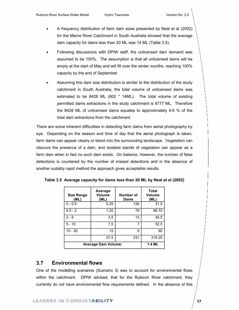
• A frequency distribution of farm dam sizes presented by Neal et al (2002)
for the Marne River Catchment in South Australia showed that the average
dam capacity for dams less than 20 ML was 14 ML (Table 3.5).
• Following discussions with DPIW staff, the unlicensed dam demand was
assumed to be 100%. The assumption is that all unlicensed dams will be
empty at the start of May and will fill over the winter months, reaching 100%
capacity by the end of September.
• Assuming this dam size distribution is similar to the distribution of the study
catchment in South Australia, the total volume of unlicensed dams was
estimated to be 8428 ML (602 * 14ML). The total volume of existing
permitted dams extractions in the study catchment is 8777 ML. Therefore
the 8428 ML of unlicensed dams equates to approximately 9.6 % of the
total dam extractions from the catchment.
There are some inherent difficulties in detecting farm dams from aerial photography by
eye. Depending on the season and time of day that the aerial photograph is taken,
farm dams can appear clearly or blend into the surrounding landscape. Vegetation can
obscure the presence of a dam, and isolated stands of vegetation can appear as a
farm dam when in fact no such dam exists. On balance, however, the number of false
detections is countered by the number of missed detections and in the absence of
another suitably rapid method the approach gives acceptable results.
Table 3.5 Average capacity for dams less than 20 ML by Neal et al (2002)
Size Range (ML)
Average Volume
(ML) Number of
Dams
Total Volume
(ML)
0 - 0.5 0.25 126 31.5
0.5 - 2 1.25 79 98.75
2 - 5 3.5 13 45.5
5 - 10 7.5 7 52.5
10 - 20 15 6 90
27.5 231 318.25
Average Dam Volume: 1.4 ML
3.7 Environmental flows
One of the modelling scenarios (Scenario 3) was to account for environmental flows
within the catchment. DPIW advised, that for the Rubicon River catchment, they
currently do not have environmental flow requirements defined. In the absence of this

Rubicon River Surface Water Model Hydro Tasmania Version No: 2.0
18
information it was agreed that the calibrated catchment model would be run in the
Modelled – No entitlements (Natural) scenario and the environmental flow would be
assumed to be:
• The 20th percentile for each sub-catchment during the winter period (01May to
31st Oct).
• The 30th percentile for each sub-catchment during the summer period (01 Nov –
30 April).
The Modelled – No entitlements (Natural) flow scenario was run from 01/01/1970 to
01/01/2007.
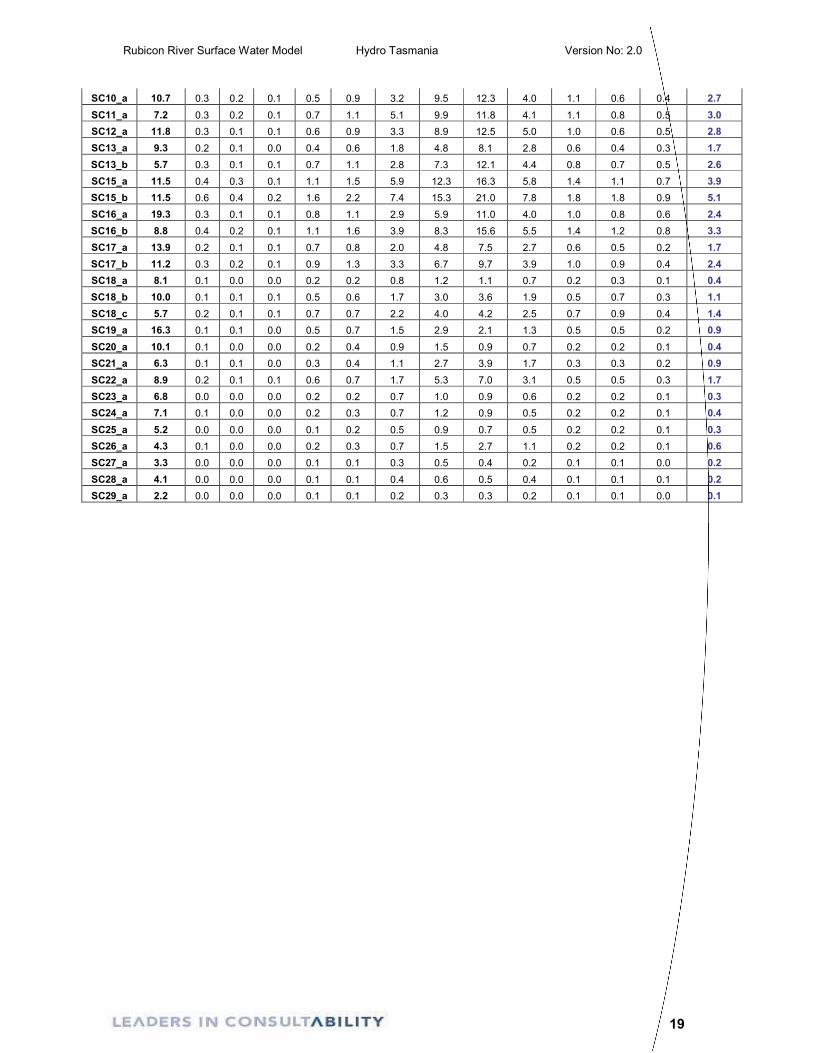
A summary table of the environmental flows on a monthly breakdown by sub-catchment
is provided in the following table and in the Catchment User Interface.
Table 3.6 Environmental Flows
Sub-Catchment Area (km2)
Environmental Flow (ML/d) Per Month at each sub-Catchment
Jan Feb Mar Apr May Jun Jul Aug Sep Oct Nov Dec Average
SC1_a 34.8 0.9 0.4 0.3 2.0 2.3 8.8 21.1 38.2 21.8 4.0 2.3 1.6 8.6
SC1_b 19.6 1.3 0.7 0.4 2.8 3.3 13.4 32.3 58.1 33.8 5.8 3.3 2.4 13.1
SC1_c 19.2 1.9 1.0 0.5 3.5 4.5 18.3 45.6 82.2 47.4 8.2 4.3 3.4 18.4
SC1_d 11.2 3.0 1.4 1.1 5.8 7.0 31.0 71.4 128.6 65.5 11.8 6.0 6.0 28.2
SC1_e 11.0 5.1 2.3 1.7 9.5 11.5 52.5 115.9 216.7 93.1 17.0 10.1 8.8 45.4
SC1_f 9.6 5.3 2.4 1.8 9.8 12.1 53.8 118.7 225.8 94.2 17.5 10.6 9.4 46.8
SC1_g 10.2 5.9 2.7 2.1 10.8 13.4 57.5 128.2 248.9 97.5 18.2 11.7 11.1 50.7
SC1_h 8.0 6.2 2.9 2.2 11.0 13.9 57.6 131.1 255.9 98.1 18.7 12.3 11.6 51.8
SC2_a 10.4 0.2 0.1 0.0 0.4 0.6 2.4 5.9 10.1 3.1 0.7 0.5 0.3 2.0
SC2_b 12.7 0.5 0.2 0.1 0.9 1.4 5.3 12.8 22.5 6.7 1.6 1.0 0.7 4.5
SC2_c 6.6 0.9 0.5 0.2 1.9 2.7 10.2 26.2 44.2 14.0 3.1 2.0 1.6 9.0
SC3_a 14.1 0.3 0.1 0.0 0.6 0.9 3.2 7.4 13.1 4.4 1.0 0.6 0.4 2.7
SC3_b 25.2 0.8 0.3 0.1 1.6 2.4 8.5 19.3 36.2 12.3 2.7 1.7 1.1 7.2
SC4_a 6.1 0.1 0.1 0.0 0.3 0.4 1.3 3.1 6.0 2.7 0.5 0.3 0.2 1.2
SC5_a 15.3 0.3 0.2 0.1 0.7 1.0 3.6 9.6 15.1 5.6 1.1 0.7 0.6 3.2
SC6_a 19.9 0.4 0.2 0.1 1.0 1.1 3.2 9.4 18.5 6.7 1.2 1.1 0.8 3.6
SC6_b 14.1 0.7 0.3 0.1 1.7 1.7 5.5 15.9 30.9 10.8 2.1 1.8 1.4 6.1
SC7_a 13.9 0.3 0.2 0.1 0.7 1.2 4.2 12.6 16.2 5.2 1.4 0.8 0.5 3.6
SC7_b 9.6 0.9 0.6 0.3 1.6 3.0 10.4 30.7 40.3 13.4 3.3 1.9 1.5 9.0
SC7_c 8.1 1.4 0.8 0.4 2.9 4.7 16.5 44.9 61.7 23.0 4.9 3.0 2.4 13.9
SC7_d 11.7 3.5 2.1 1.1 8.2 12.2 48.0 108.1 144.0 63.4 11.1 10.0 6.4 34.8
SC7_e 8.6 3.7 2.2 1.1 9.2 12.8 49.2 111.3 150.5 67.3 11.8 10.5 6.9 36.4
SC7_f 10.0 4.0 2.3 1.2 10.4 13.6 50.5 115.0 157.9 71.8 12.6 11.1 7.4 38.2
SC7_g 1.5 3.9 2.3 1.3 10.5 13.7 50.3 115.3 158.7 72.7 12.7 11.3 7.5 38.4
SC8_a 12.1 0.4 0.3 0.1 1.0 1.5 6.4 12.9 17.1 6.4 1.3 1.2 0.7 4.1
SC8_b 10.7 1.0 0.7 0.3 2.5 3.8 16.1 32.5 43.2 16.9 3.4 3.1 1.8 10.4
SC8_c 10.9 1.7 1.1 0.6 4.2 6.3 26.9 53.3 70.0 27.0 6.0 5.0 3.0 17.1
SC9_a 7.9 0.2 0.1 0.1 0.5 0.8 3.4 7.9 10.1 4.1 0.8 0.6 0.4 2.4
Rubicon River Surface Water Model Hydro Tasmania Version No: 2.0
19
SC10_a 10.7 0.3 0.2 0.1 0.5 0.9 3.2 9.5 12.3 4.0 1.1 0.6 0.4 2.7
SC11_a 7.2 0.3 0.2 0.1 0.7 1.1 5.1 9.9 11.8 4.1 1.1 0.8 0.5 3.0
SC12_a 11.8 0.3 0.1 0.1 0.6 0.9 3.3 8.9 12.5 5.0 1.0 0.6 0.5 2.8
SC13_a 9.3 0.2 0.1 0.0 0.4 0.6 1.8 4.8 8.1 2.8 0.6 0.4 0.3 1.7
SC13_b 5.7 0.3 0.1 0.1 0.7 1.1 2.8 7.3 12.1 4.4 0.8 0.7 0.5 2.6
SC15_a 11.5 0.4 0.3 0.1 1.1 1.5 5.9 12.3 16.3 5.8 1.4 1.1 0.7 3.9
SC15_b 11.5 0.6 0.4 0.2 1.6 2.2 7.4 15.3 21.0 7.8 1.8 1.8 0.9 5.1
SC16_a 19.3 0.3 0.1 0.1 0.8 1.1 2.9 5.9 11.0 4.0 1.0 0.8 0.6 2.4
SC16_b 8.8 0.4 0.2 0.1 1.1 1.6 3.9 8.3 15.6 5.5 1.4 1.2 0.8 3.3
SC17_a 13.9 0.2 0.1 0.1 0.7 0.8 2.0 4.8 7.5 2.7 0.6 0.5 0.2 1.7
SC17_b 11.2 0.3 0.2 0.1 0.9 1.3 3.3 6.7 9.7 3.9 1.0 0.9 0.4 2.4
SC18_a 8.1 0.1 0.0 0.0 0.2 0.2 0.8 1.2 1.1 0.7 0.2 0.3 0.1 0.4
SC18_b 10.0 0.1 0.1 0.1 0.5 0.6 1.7 3.0 3.6 1.9 0.5 0.7 0.3 1.1
SC18_c 5.7 0.2 0.1 0.1 0.7 0.7 2.2 4.0 4.2 2.5 0.7 0.9 0.4 1.4
SC19_a 16.3 0.1 0.1 0.0 0.5 0.7 1.5 2.9 2.1 1.3 0.5 0.5 0.2 0.9
SC20_a 10.1 0.1 0.0 0.0 0.2 0.4 0.9 1.5 0.9 0.7 0.2 0.2 0.1 0.4
SC21_a 6.3 0.1 0.1 0.0 0.3 0.4 1.1 2.7 3.9 1.7 0.3 0.3 0.2 0.9
SC22_a 8.9 0.2 0.1 0.1 0.6 0.7 1.7 5.3 7.0 3.1 0.5 0.5 0.3 1.7
SC23_a 6.8 0.0 0.0 0.0 0.2 0.2 0.7 1.0 0.9 0.6 0.2 0.2 0.1 0.3
SC24_a 7.1 0.1 0.0 0.0 0.2 0.3 0.7 1.2 0.9 0.5 0.2 0.2 0.1 0.4
SC25_a 5.2 0.0 0.0 0.0 0.1 0.2 0.5 0.9 0.7 0.5 0.2 0.2 0.1 0.3
SC26_a 4.3 0.1 0.0 0.0 0.2 0.3 0.7 1.5 2.7 1.1 0.2 0.2 0.1 0.6
SC27_a 3.3 0.0 0.0 0.0 0.1 0.1 0.3 0.5 0.4 0.2 0.1 0.1 0.0 0.2
SC28_a 4.1 0.0 0.0 0.0 0.1 0.1 0.4 0.6 0.5 0.4 0.1 0.1 0.1 0.2
SC29_a 2.2 0.0 0.0 0.0 0.1 0.1 0.2 0.3 0.3 0.2 0.1 0.1 0.0 0.1
Rubicon River Surface Water Model Hydro Tasmania Version No: 2.0
20
4. MODEL DEVELOPMENT
4.1 Sub-catchment delineation
Sub-catchment delineation was performed using CatchmentSIM GIS software.
CatchmentSIM is a 3D-GIS topographic parameterisation and hydrologic analysis model.
The model automatically delineates watershed and sub-catchment boundaries,
generalises geophysical parameters and provides in-depth analysis tools to examine and
compare the hydrologic properties of sub-catchments. The model also includes a flexible
result export macro language to allow users to fully couple CatchmentSIM with any
hydrologic modelling package that is based on sub-catchment networks.
For the purpose of this project, CatchmentSIM was used to delineate the catchment,
break it up into numerous sub-catchments, determine their areas and provide routing
lengths between them.
These outputs were manually checked to ensure they accurately represented the
catchment. If any minor modifications were required these were made manually to the
resulting model.
For more detailed information on CatchmentSIM see the CatchmentSIM Homepage
www.toolkit.net.au/catchsim/
4.2 Hydstra Model
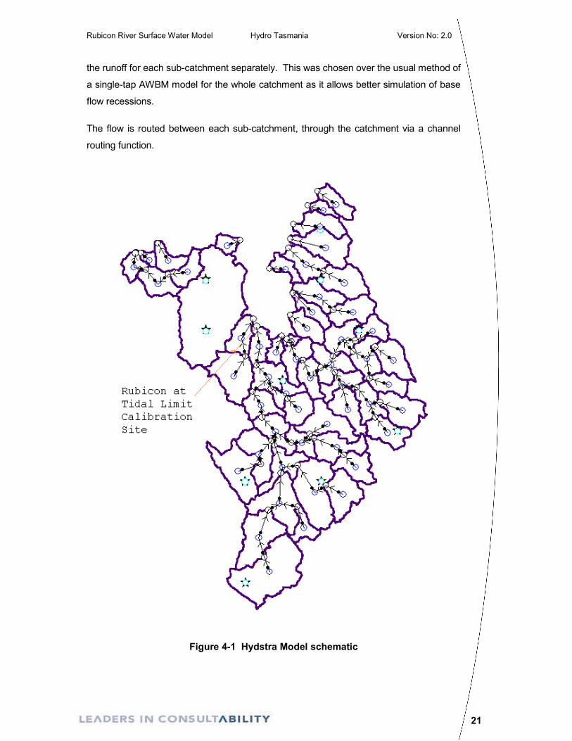
A computer simulation model was developed using Hydstra Modelling. The sub-
catchments, described in Figure 2-1, were represented by model “nodes” and
connected together by “links”. A schematic of this model is displayed in Figure 4-1.
The flow is routed between each sub-catchment, through the catchment via a channel
routing function.
The rainfall and evaporation is calculated for each sub-catchment using inverse-
distance gauge weighting. The gauge weights were automatically calculated at the
start of each model run. The weighting is computed for the centroid of the sub-
catchment. A quadrant system is drawn, centred on the centroid. A weight for the
closest gauge in each quadrant is computed as the inverse, squared, distance between
the gauge and centroid. For each time step and each node, the gauge weights are
applied to the incoming rainfall and evaporation data.
The AWBM Two Tap rainfall/runoff model (Parkyn & Wilson 1997) was used to calculate
Rubicon River Surface Water Model Hydro Tasmania Version No: 2.0
21
the runoff for each sub-catchment separately. This was chosen over the usual method of
a single-tap AWBM model for the whole catchment as it allows better simulation of base
flow recessions.
The flow is routed between each sub-catchment, through the catchment via a channel
routing function.
Figure 4-1 Hydstra Model schematic
Rubicon River Surface Water Model Hydro Tasmania Version No: 2.0
22
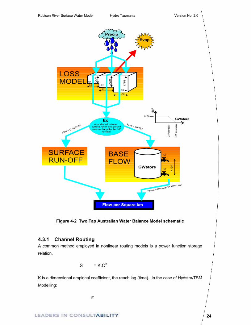
4.3 AWBM Model
The AWBM Two Tap model (Parkyn & Wilson 1997) is a relatively simple water balance
model with the following characteristics:
• it has few parameters to fit,
• the model representation is easily understood in terms of the actual outflow
hydrograph,
• the parameters of the model can largely be determined by analysis of the
outflow hydrograph,
• the model accounts for partial area rainfall-run-off effects,
• runoff volume is relatively insensitive to the model parameters.
For these reasons parameters can more easily be transferred to ungauged catchments.
The AWBM routine used in this study is the Boughton Revised AWBM model (Boughton,
2003), which reduces the three partial areas and three surface storage capacities to
relationships based on an average surface storage capacity.
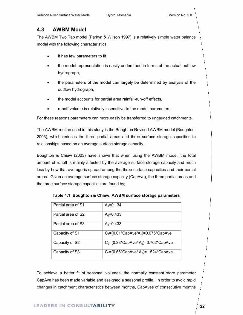
Boughton & Chiew (2003) have shown that when using the AWBM model, the total
amount of runoff is mainly affected by the average surface storage capacity and much
less by how that average is spread among the three surface capacities and their partial
areas. Given an average surface storage capacity (CapAve), the three partial areas and
the three surface storage capacities are found by;
Table 4.1 Boughton & Chiew, AWBM surface storage parameters
Partial area of S1 A1=0.134
Partial area of S2 A2=0.433
Partial area of S3 A3=0.433
Capacity of S1 C1=(0.01*CapAve/A1)=0.075*CapAve
Capacity of S2 C2=(0.33*CapAve/ A2)=0.762*CapAve
Capacity of S3 C3=(0.66*CapAve/ A3)=1.524*CapAve
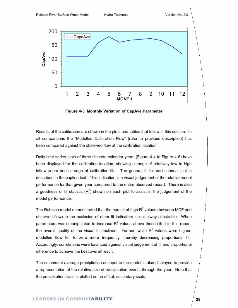
To achieve a better fit of seasonal volumes, the normally constant store parameter
CapAve has been made variable and assigned a seasonal profile. In order to avoid rapid
changes in catchment characteristics between months, CapAves of consecutive months
Rubicon River Surface Water Model Hydro Tasmania Version No: 2.0
23
were smoothed. A CapAve of a given month was assumed to occur on the middle day of
that month. It was assumed that daily CapAves occurring between consecutive monthly
CapAves would fit to a straight line, and a CapAve for each day was calculated on this
basis. The annual profile of CapAves for the catchment is shown in Figure 4-3.
The AWBM routine produces two outputs; direct run-off and base-flow. Direct run-off is
produced after the content of any of the soil stores is exceeded; it can be applied to the
stream network directly or by catchment routing across each subcatchment. Base-flow is
usually supplied unrouted directly to the stream network, at a rate proportional to the
water depth in the ground water store. The ground water store is recharged from a
proportion of excess rainfall from the three surface soil storages.
Whilst the AWBM methodology incorporates an account of base-flow, it is not intended
that the baseflow prediction from the AWBM model be adopted as an accurate estimate
of the baseflow contribution. The base flow in the AWBM routine is based on a simple
model and does not specifically account for attributes that affect baseflow such as
geology and inter-catchment ground water transfers. During the model calibration the
baseflow infiltration and recession parameters are used to ensure a reasonable fit with
the observed surface water information.
The AWBM processes are shown in the following Figure 4-2;
Rubicon River Surface Water Model Hydro Tasmania Version No: 2.0
24
Figure 4-2 Two Tap Australian Water Balance Model schematic
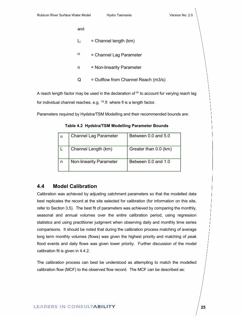
4.3.1 Channel Routing
A common method employed in nonlinear routing models is a power function storage
relation.
S = K.Qn
K is a dimensional empirical coefficient, the reach lag (time). In the case of Hydstra/TSM
Modelling:
α
Rubicon River Surface Water Model Hydro Tasmania Version No: 2.0
25
and
Li = Channel length (km)
α = Channel Lag Parameter
n = Non-linearity Parameter
Q = Outflow from Channel Reach (m3/s)
A reach length factor may be used in the declaration of α to account for varying reach lag
for individual channel reaches. e.g. α.fl where fl is a length factor.
Parameters required by Hydstra/TSM Modelling and their recommended bounds are:
Table 4.2 Hydstra/TSM Modelling Parameter Bounds
α Channel Lag Parameter Between 0.0 and 5.0
L Channel Length (km) Greater than 0.0 (km)
n Non-linearity Parameter Between 0.0 and 1.0
4.4 Model Calibration
Calibration was achieved by adjusting catchment parameters so that the modelled data
best replicates the record at the site selected for calibration (for information on this site,
refer to Section 3.5). The best fit of parameters was achieved by comparing the monthly,
seasonal and annual volumes over the entire calibration period, using regression
statistics and using practitioner judgment when observing daily and monthly time series
comparisons. It should be noted that during the calibration process matching of average
long term monthly volumes (flows) was given the highest priority and matching of peak
flood events and daily flows was given lower priority. Further discussion of the model
calibration fit is given in 4.4.2.
The calibration process can best be understood as attempting to match the modelled
calibration flow (MCF) to the observed flow record. The MCF can be described as:
Rubicon River Surface Water Model Hydro Tasmania Version No: 2.0
26
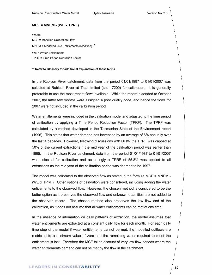
MCF = MNEM - (WE x TPRF)
Where:
MCF = Modelled Calibration Flow
MNEM = Modelled - No Entitlements (Modified). *
WE = Water Entitlements
TPRF = Time Period Reduction Factor
* Refer to Glossary for additional explanation of these terms
In the Rubicon River catchment, data from the period 01/01/1987 to 01/01/2007 was
selected at Rubicon River at Tidal limited (site 17200) for calibration. It is generally
preferable to use the most recent flows available. While the record extended to October
2007, the latter few months were assigned a poor quality code, and hence the flows for
2007 were not included in the calibration period.
Water entitlements were included in the calibration model and adjusted to the time period
of calibration by applying a Time Period Reduction Factor (TPRF). The TPRF was
calculated by a method developed in the Tasmanian State of the Environment report
(1996). This states that water demand has increased by an average of 6% annually over
the last 4 decades. However, following discussions with DPIW the TPRF was capped at
50% of the current extractions if the mid year of the calibration period was earlier than
1995. In the Rubicon River catchment, data from the period 01/01/1987 to 01/01/2007
was selected for calibration and accordingly a TPRF of 55.8% was applied to all
extractions as the mid year of the calibration period was deemed to be 1997.
The model was calibrated to the observed flow as stated in the formula MCF = MNEM -
(WE x TPRF). Other options of calibration were considered, including adding the water
entitlements to the observed flow. However, the chosen method is considered to be the
better option as it preserves the observed flow and unknown quantities are not added to
the observed record. The chosen method also preserves the low flow end of the
calibration, as it does not assume that all water entitlements can be met at any time.
In the absence of information on daily patterns of extraction, the model assumes that
water entitlements are extracted at a constant daily flow for each month. For each daily
time step of the model if water entitlements cannot be met, the modelled outflows are
restricted to a minimum value of zero and the remaining water required to meet the
entitlement is lost. Therefore the MCF takes account of very low flow periods where the
water entitlements demand can not be met by the flow in the catchment.
Rubicon River Surface Water Model Hydro Tasmania Version No: 2.0
27
Table 4.4 shows the monthly water entitlements (demand) used in the model calibration
upstream of the calibration site.
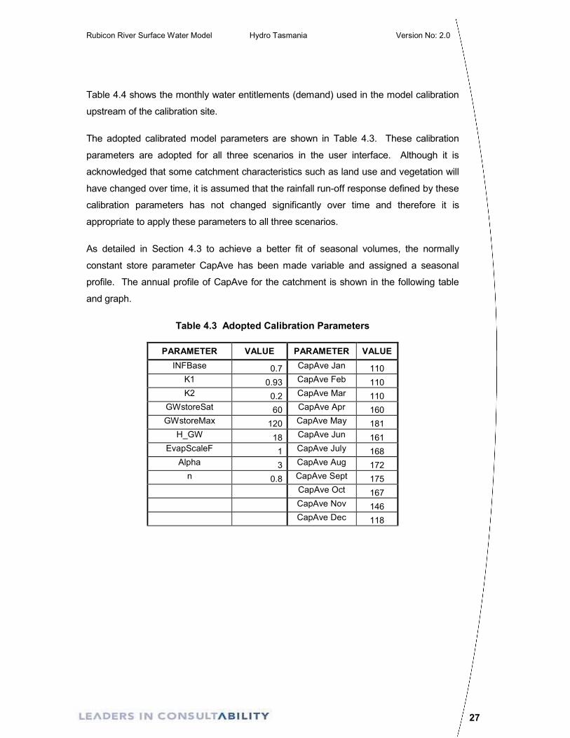
The adopted calibrated model parameters are shown in Table 4.3. These calibration
parameters are adopted for all three scenarios in the user interface. Although it is
acknowledged that some catchment characteristics such as land use and vegetation will
have changed over time, it is assumed that the rainfall run-off response defined by these
calibration parameters has not changed significantly over time and therefore it is
appropriate to apply these parameters to all three scenarios.
As detailed in Section 4.3 to achieve a better fit of seasonal volumes, the normally
constant store parameter CapAve has been made variable and assigned a seasonal
profile. The annual profile of CapAve for the catchment is shown in the following table
and graph.
Table 4.3 Adopted Calibration Parameters
PARAMETER VALUE PARAMETER VALUE
INFBase 0.7 CapAve Jan 110
K1 0.93 CapAve Feb 110
K2 0.2 CapAve Mar 110
GWstoreSat 60 CapAve Apr 160
GWstoreMax 120 CapAve May 181
H_GW 18 CapAve Jun 161
EvapScaleF 1 CapAve July 168
Alpha 3 CapAve Aug 172
n 0.8 CapAve Sept 175
CapAve Oct 167
CapAve Nov 146
CapAve Dec 118
Rubicon River Surface Water Model Hydro Tasmania Version No: 2.0
28
0
50
100
150
200
1 2 3 4 5 6 7 8 9 10 11 12MONTH
CapA
ve
CapeAve
Figure 4-3 Monthly Variation of CapAve Parameter
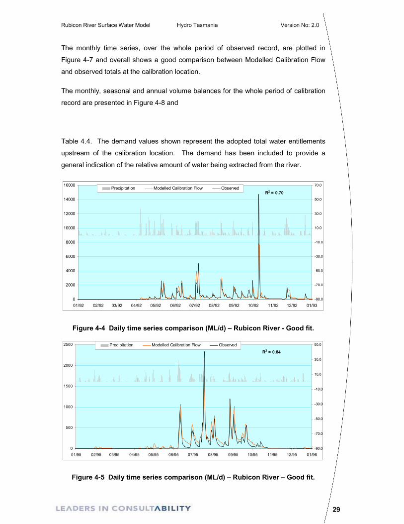
Results of the calibration are shown in the plots and tables that follow in this section. In
all comparisons the “Modelled Calibration Flow” (refer to previous description) has
been compared against the observed flow at the calibration location.
Daily time series plots of three discrete calendar years (Figure 4-4 to Figure 4-6) have
been displayed for the calibration location, showing a range of relatively low to high
inflow years and a range of calibration fits. The general fit for each annual plot is
described in the caption text. This indication is a visual judgement of the relative model
performance for that given year compared to the entire observed record. There is also
a goodness of fit statistic (R2) shown on each plot to assist in the judgement of the
model performance.
The Rubicon model demonstrated that the pursuit of high R2 values (between MCF and
observed flow) to the exclusion of other fit indicators is not always desirable. When
parameters were manipulated to increase R2 values above those cited in this report,
the overall quality of the visual fit declined. Further, while R2 values were higher,
modelled flow fell to zero more frequently, thereby decreasing proportional fit.
Accordingly, correlations were balanced against visual judgement of fit and proportional
difference to achieve the best overall result.
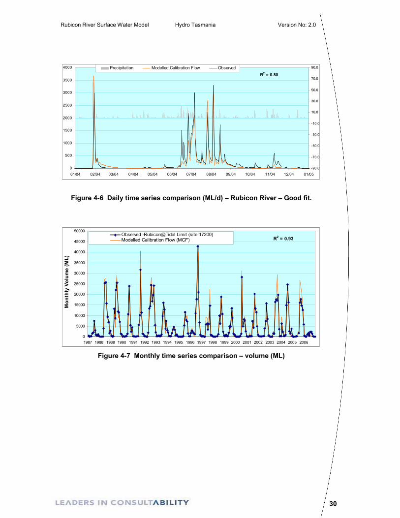
The catchment average precipitation as input to the model is also displayed to provide
a representation of the relative size of precipitation events through the year. Note that
the precipitation trace is plotted on an offset, secondary scale.
Rubicon River Surface Water Model Hydro Tasmania Version No: 2.0
29
The monthly time series, over the whole period of observed record, are plotted in
Figure 4-7 and overall shows a good comparison between Modelled Calibration Flow
and observed totals at the calibration location.
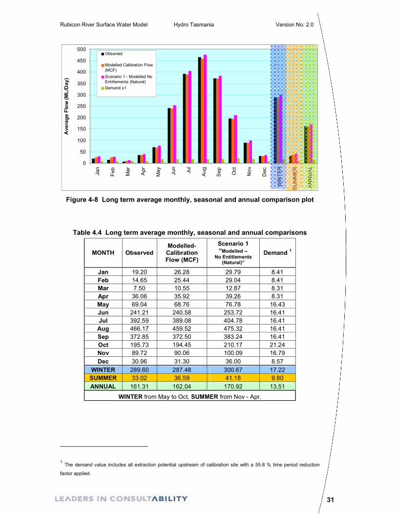
The monthly, seasonal and annual volume balances for the whole period of calibration
record are presented in Figure 4-8 and
Table 4.4. The demand values shown represent the adopted total water entitlements
upstream of the calibration location. The demand has been included to provide a
general indication of the relative amount of water being extracted from the river.
0
2000
4000
6000
8000
10000
12000
14000
16000
01/92 02/92 03/92 04/92 05/92 06/92 07/92 08/92 09/92 10/92 11/92 12/92 01/93
-90.0
-70.0
-50.0
-30.0
-10.0
10.0
30.0
50.0
70.0Precipitation Modelled Calibration Flow Observed
R2 = 0.70
Figure 4-4 Daily time series comparison (ML/d) – Rubicon River - Good fit.
0
500
1000
1500
2000
2500
01/95 02/95 03/95 04/95 05/95 06/95 07/95 08/95 09/95 10/95 11/95 12/95 01/96
-90.0
-70.0
-50.0
-30.0
-10.0
10.0
30.0
50.0Precipitation Modelled Calibration Flow Observed
R2 = 0.84
Figure 4-5 Daily time series comparison (ML/d) – Rubicon River – Good fit.
Rubicon River Surface Water Model Hydro Tasmania Version No: 2.0
30
0
500
1000
1500
2000
2500
3000
3500
4000
01/04 02/04 03/04 04/04 05/04 06/04 07/04 08/04 09/04 10/04 11/04 12/04 01/05
-90.0
-70.0
-50.0
-30.0
-10.0
10.0
30.0
50.0
70.0
90.0Precipitation Modelled Calibration Flow Observed
R2 = 0.80
Figure 4-6 Daily time series comparison (ML/d) – Rubicon River – Good fit.
0
5000
10000
15000
20000
25000
30000
35000
40000
45000
50000
1987 1988 1988 1990 1991 1992 1993 1994 1995 1996 1997 1998 1999 2000 2001 2002 2003 2004 2005 2006
Month
ly V
olu
me (M
L)
Observed -Rubicon@Tidal Limit (site 17200)Modelled Calibration Flow (MCF) R2 = 0.93
Figure 4-7 Monthly time series comparison – volume (ML)
Rubicon River Surface Water Model Hydro Tasmania Version No: 2.0
31
0
50
100
150
200
250
300
350
400
450
500
Jan
Feb
Mar
Apr
May
Jun
Jul
Aug
Sep
Oct
Nov
Dec
WINTER
SUMMER
ANNUAL
Avera
ge F
low
(M
L/D
ay)
Observed
Modelled Calibration Flow
(MCF)
Scenario 1 - Modelled No
Entitlements (Natural)
Demand x1
Figure 4-8 Long term average monthly, seasonal and annual comparison plot
Table 4.4 Long term average monthly, seasonal and annual comparisons
MONTH Observed Modelled- Calibration Flow (MCF)
Scenario 1 “Modelled --
No Entitlements (Natural)”
Demand 1
Jan 19.20 26.28 29.79 8.41
Feb 14.65 25.44 29.04 8.41
Mar 7.50 10.55 12.87 8.31
Apr 36.06 35.92 39.26 8.31
May 69.04 68.76 76.78 16.43
Jun 241.21 240.58 253.72 16.41
Jul 392.59 389.08 404.78 16.41
Aug 466.17 459.52 475.32 16.41
Sep 372.85 372.50 383.24 16.41
Oct 195.73 194.45 210.17 21.24
Nov 89.72 90.06 100.09 16.79
Dec 30.96 31.30 36.00 8.57
WINTER 289.60 287.48 300.67 17.22
SUMMER 33.02 36.59 41.18 9.80
ANNUAL 161.31 162.04 170.92 13.51
WINTER from May to Oct, SUMMER from Nov - Apr.
1 The demand value includes all extraction potential upstream of calibration site with a 55.8 % time period reduction
factor applied.
Rubicon River Surface Water Model Hydro Tasmania Version No: 2.0
32
4.4.1 Factors affecting the reliability of the model calibration.
Regardless of the effort undertaken to prepare and calibrate a model, there are always
factors which will limit the accuracy of the output. In preparation of this model the most
significant limitations that affect the accuracy of the calibration are:
1. The assumption that water entitlements are taken as a constant rate for each
month. Historically the actual extraction from the river would be much more
variable than this and possess too many levels of complexity to be accurately
represented in a model.
2. The current quantity of water extracted from the catchment is unknown. Although
DPIW have provided water licence information (WIMS July 2007) and estimates of
extractions in excess of these licences, these may not represent the true quantity of
water extracted. No comprehensive continuous water use data is currently
available.
3. The quality of the observed flow data (ratings and water level readings) used in the
calibration may not be reliable for all periods. Even for sites where reliable data
and ratings has been established the actual flow may still be significantly different
to the observed (recorded) data, due to the inherent difficulties in recording
accurate height data and rating it to flow. These errors typically increase in periods
of low and high flows.
4. Misrepresentation of the catchment precipitation. This is due to insufficient rainfall
gauge information in and around the catchment. Despite the Data DRILL’s good
coverage of grid locations, the development of this grid information would still rely
considerably on the availability of measured rainfall information in the region. This
would also be the case with the evaporation data, which will have a smaller impact
on the calibration.
5. The daily average timestep of the model may smooth out rainfall temporal patterns
and have an effect on the peak flows. For example, intense rainfall events falling in
a few hours will be represented as a daily average rainfall, accordingly reducing the
peak flow.
6. The model does not explicitly account for changes in vegetation and terrain within
individual sub-catchments. Effects due to vegetation and terrain are accounted for
on catchment average basis, using the global AWBM fit parameters. Therefore
individual sub-catchment run-off may not be accurately represented by the model’s
Rubicon River Surface Water Model Hydro Tasmania Version No: 2.0
33
global fit parameters. To account for this a much more detailed and complex model
would be required.
4.4.2 Model Accuracy - Model Fit Statistics
The following section is an additional assessment of how reliably the model predicts
flow at the calibration site.
One of the most common measures of comparison between two sets of data is the
coefficient of determination (R2). If two data sets are defined as x and y, R2 is the
variance in y attributable to the variance in x. A high R2 value indicates that x and y
vary together – that is, the two data sets have a good correlation. In this case x and y
are observed flow and modelled calibration flow. So for the catchment model, R2
indicates how much the modelled calibration flow changes as observed flow changes.
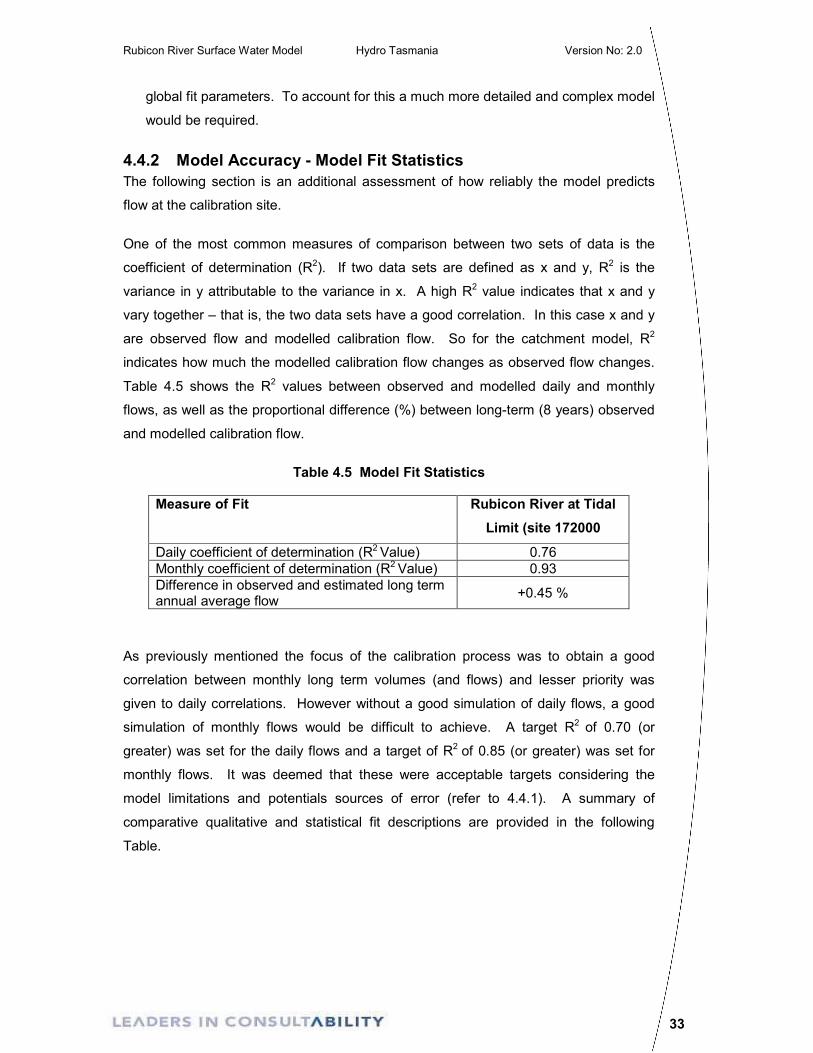
Table 4.5 shows the R2 values between observed and modelled daily and monthly
flows, as well as the proportional difference (%) between long-term (8 years) observed
and modelled calibration flow.
Table 4.5 Model Fit Statistics
Measure of Fit Rubicon River at Tidal
Limit (site 172000
Daily coefficient of determination (R2 Value) 0.76
Monthly coefficient of determination (R2 Value) 0.93
Difference in observed and estimated long term annual average flow
+0.45 %
As previously mentioned the focus of the calibration process was to obtain a good
correlation between monthly long term volumes (and flows) and lesser priority was
given to daily correlations. However without a good simulation of daily flows, a good
simulation of monthly flows would be difficult to achieve. A target R2 of 0.70 (or
greater) was set for the daily flows and a target of R2 of 0.85 (or greater) was set for
monthly flows. It was deemed that these were acceptable targets considering the
model limitations and potentials sources of error (refer to 4.4.1). A summary of
comparative qualitative and statistical fit descriptions are provided in the following
Table.
Rubicon River Surface Water Model Hydro Tasmania Version No: 2.0
34
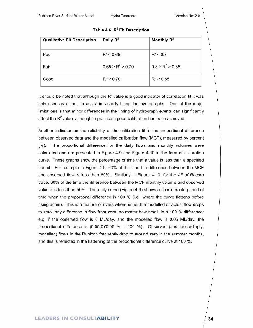
Table 4.6 R2 Fit Description
Qualitative Fit Description Daily R2 Monthly R2
Poor R2 < 0.65 R2 < 0.8
Fair 0.65 ≥ R2 > 0.70 0.8 ≥ R2 > 0.85
Good R2 ≥ 0.70 R2 ≥ 0.85
It should be noted that although the R2 value is a good indicator of correlation fit it was
only used as a tool, to assist in visually fitting the hydrographs. One of the major
limitations is that minor differences in the timing of hydrograph events can significantly
affect the R2 value, although in practice a good calibration has been achieved.
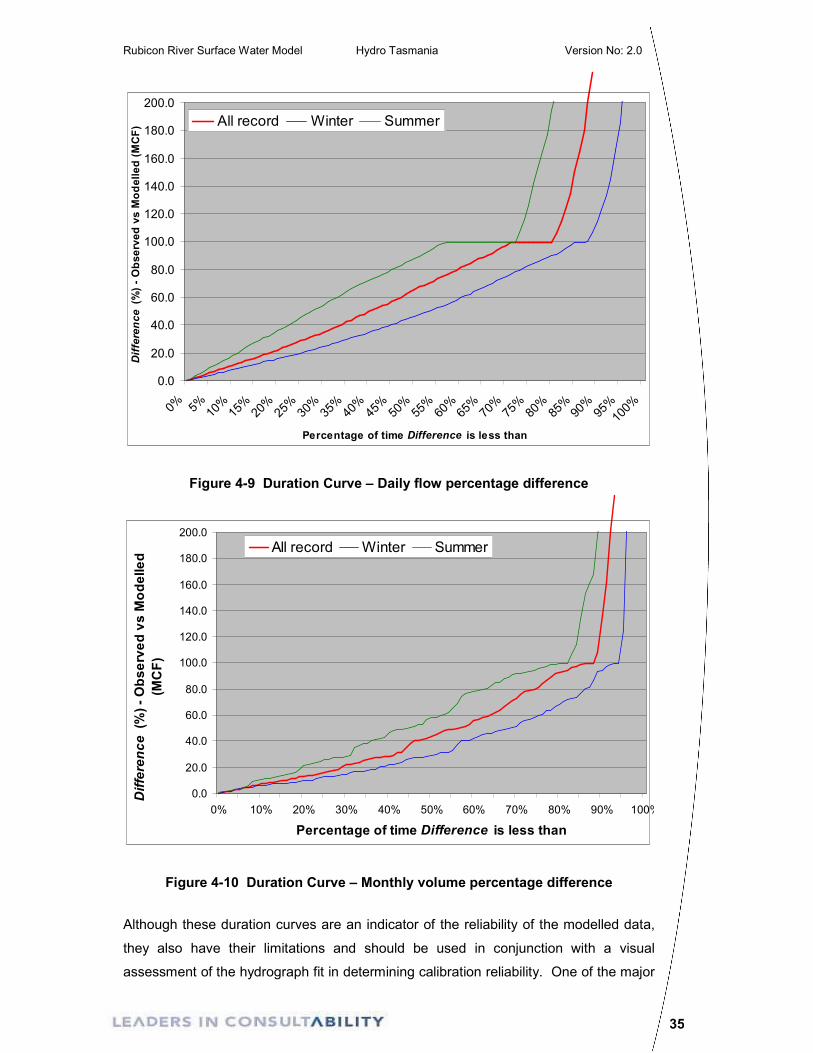
Another indicator on the reliability of the calibration fit is the proportional difference
between observed data and the modelled calibration flow (MCF), measured by percent
(%). The proportional difference for the daily flows and monthly volumes were
calculated and are presented in Figure 4-9 and Figure 4-10 in the form of a duration
curve. These graphs show the percentage of time that a value is less than a specified
bound. For example in Figure 4-9, 60% of the time the difference between the MCF
and observed flow is less than 80%. Similarly in Figure 4-10, for the All of Record
trace, 60% of the time the difference between the MCF monthly volume and observed
volume is less than 50%. The daily curve (Figure 4-9) shows a considerable period of
time when the proportional difference is 100 % (i.e., where the curve flattens before
rising again). This is a feature of rivers where either the modelled or actual flow drops
to zero (any difference in flow from zero, no matter how small, is a 100 % difference:
e.g. if the observed flow is 0 ML/day, and the modelled flow is 0.05 ML/day, the
proportional difference is (0.05-0)/0.05 % = 100 %). Observed (and, accordingly,
modelled) flows in the Rubicon frequently drop to around zero in the summer months,
and this is reflected in the flattening of the proportional difference curve at 100 %.
Rubicon River Surface Water Model Hydro Tasmania Version No: 2.0
35
0.0
20.0
40.0
60.0
80.0
100.0
120.0
140.0
160.0
180.0
200.0
0% 5% 10%15%20%25%30%35%40%45%50%55%60%65%70%75%80%85%90%95%100%
Percentage of time Difference is less than
Difference
(%
) - O
bserv
ed v
s M
odelled (M
CF) All record Winter Summer
Figure 4-9 Duration Curve – Daily flow percentage difference
0.0
20.0
40.0
60.0
80.0
100.0
120.0
140.0
160.0
180.0
200.0
0% 10% 20% 30% 40% 50% 60% 70% 80% 90% 100%
Percentage of time Difference is less than
Difference
(%
) - O
bserv
ed v
s M
odelled
(MC
F)
All record Winter Summer
Figure 4-10 Duration Curve – Monthly volume percentage difference
Although these duration curves are an indicator of the reliability of the modelled data,
they also have their limitations and should be used in conjunction with a visual
assessment of the hydrograph fit in determining calibration reliability. One of the major
Rubicon River Surface Water Model Hydro Tasmania Version No: 2.0
36
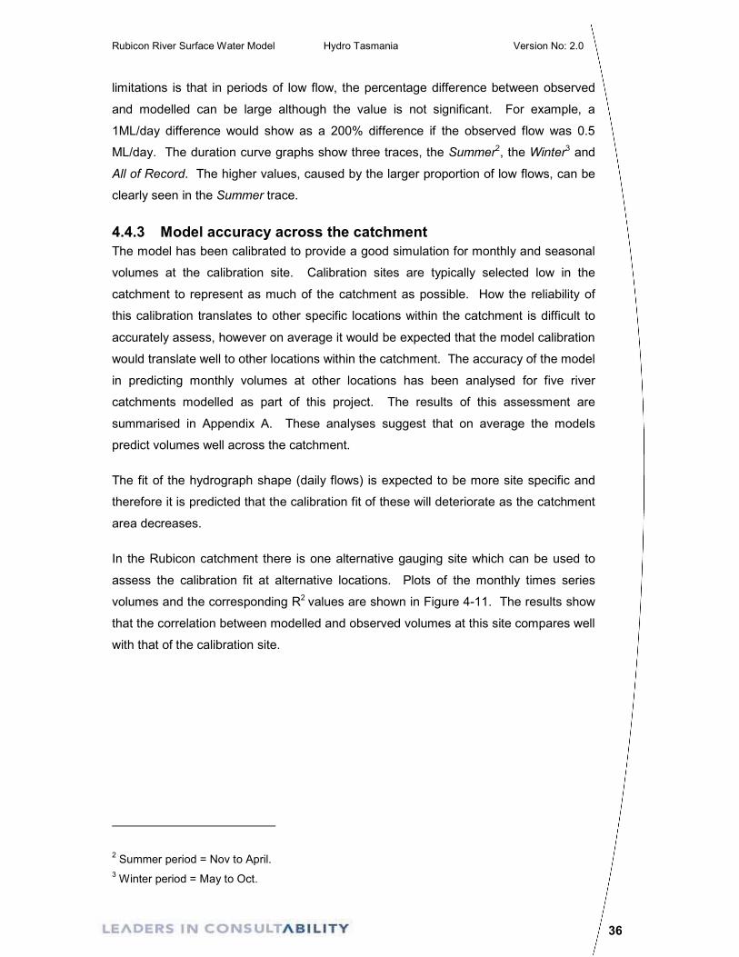
limitations is that in periods of low flow, the percentage difference between observed
and modelled can be large although the value is not significant. For example, a
1ML/day difference would show as a 200% difference if the observed flow was 0.5
ML/day. The duration curve graphs show three traces, the Summer2, the Winter3 and
All of Record. The higher values, caused by the larger proportion of low flows, can be
clearly seen in the Summer trace.
4.4.3 Model accuracy across the catchment
The model has been calibrated to provide a good simulation for monthly and seasonal
volumes at the calibration site. Calibration sites are typically selected low in the
catchment to represent as much of the catchment as possible. How the reliability of
this calibration translates to other specific locations within the catchment is difficult to
accurately assess, however on average it would be expected that the model calibration
would translate well to other locations within the catchment. The accuracy of the model
in predicting monthly volumes at other locations has been analysed for five river
catchments modelled as part of this project. The results of this assessment are
summarised in Appendix A. These analyses suggest that on average the models
predict volumes well across the catchment.
The fit of the hydrograph shape (daily flows) is expected to be more site specific and
therefore it is predicted that the calibration fit of these will deteriorate as the catchment
area decreases.
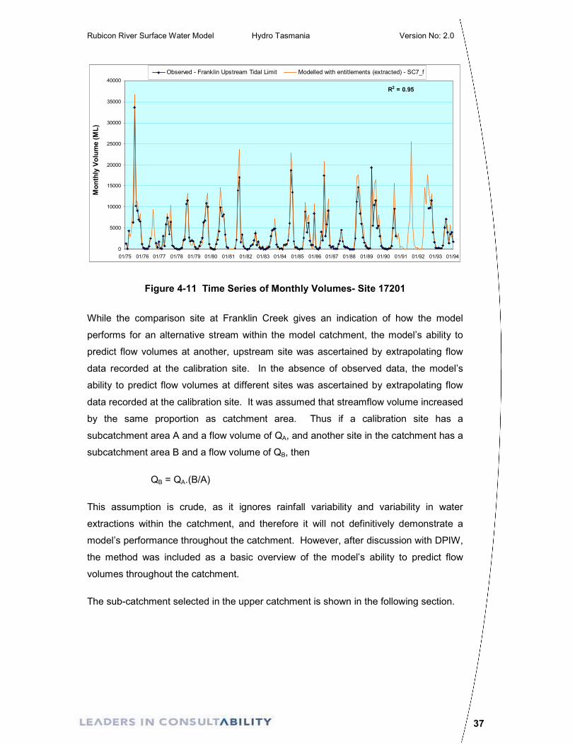
In the Rubicon catchment there is one alternative gauging site which can be used to
assess the calibration fit at alternative locations. Plots of the monthly times series
volumes and the corresponding R2 values are shown in Figure 4-11. The results show
that the correlation between modelled and observed volumes at this site compares well
with that of the calibration site.
2 Summer period = Nov to April.
3 Winter period = May to Oct.
Rubicon River Surface Water Model Hydro Tasmania Version No: 2.0
37
0
5000
10000
15000
20000
25000
30000
35000
40000
01/75 01/76 01/77 01/78 01/79 01/80 01/81 01/82 01/83 01/84 01/85 01/86 01/87 01/88 01/89 01/90 01/91 01/92 01/93 01/94
Month
ly V
olu
me (M
L)
Observed - Franklin Upstream Tidal Limit Modelled with entitlements (extracted) - SC7_f
R2 = 0.95
Figure 4-11 Time Series of Monthly Volumes- Site 17201
While the comparison site at Franklin Creek gives an indication of how the model
performs for an alternative stream within the model catchment, the model’s ability to
predict flow volumes at another, upstream site was ascertained by extrapolating flow
data recorded at the calibration site. In the absence of observed data, the model’s
ability to predict flow volumes at different sites was ascertained by extrapolating flow
data recorded at the calibration site. It was assumed that streamflow volume increased
by the same proportion as catchment area. Thus if a calibration site has a
subcatchment area A and a flow volume of QA, and another site in the catchment has a
subcatchment area B and a flow volume of QB, then
QB = QA.(B/A)
This assumption is crude, as it ignores rainfall variability and variability in water
extractions within the catchment, and therefore it will not definitively demonstrate a
model’s performance throughout the catchment. However, after discussion with DPIW,
the method was included as a basic overview of the model’s ability to predict flow
volumes throughout the catchment.
The sub-catchment selected in the upper catchment is shown in the following section.
Rubicon River Surface Water Model Hydro Tasmania Version No: 2.0
38
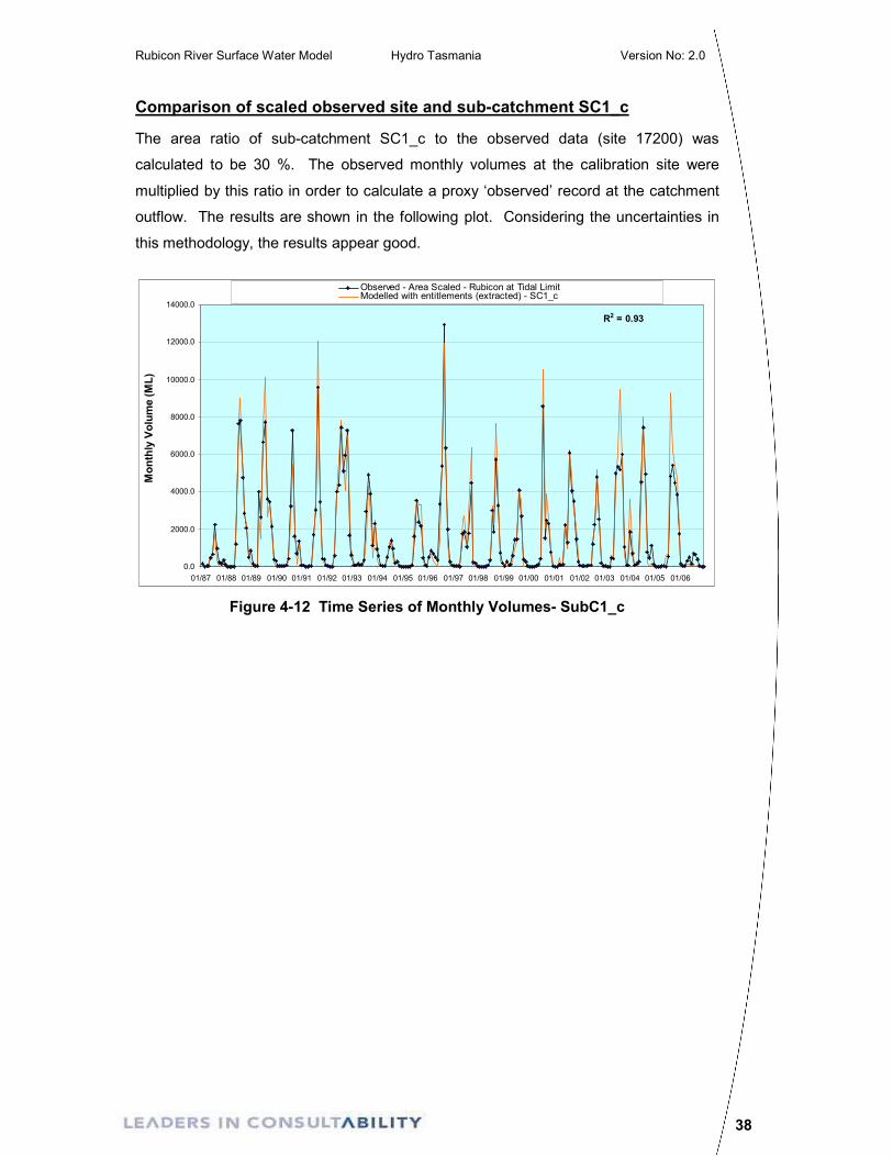
Comparison of scaled observed site and sub-catchment SC1_c
The area ratio of sub-catchment SC1_c to the observed data (site 17200) was
calculated to be 30 %. The observed monthly volumes at the calibration site were
multiplied by this ratio in order to calculate a proxy ‘observed’ record at the catchment
outflow. The results are shown in the following plot. Considering the uncertainties in
this methodology, the results appear good.
0.0
2000.0
4000.0
6000.0
8000.0
10000.0
12000.0
14000.0
01/87 01/88 01/89 01/90 01/91 01/92 01/93 01/94 01/95 01/96 01/97 01/98 01/99 01/00 01/01 01/02 01/03 01/04 01/05 01/06
Month
ly V
olu
me (M
L)
Observed - Area Scaled - Rubicon at Tidal LimitModelled with entitlements (extracted) - SC1_c
R2 = 0.93
Figure 4-12 Time Series of Monthly Volumes- SubC1_c
Rubicon River Surface Water Model Hydro Tasmania Version No: 2.0
39
5. MODEL RESULTS
The completed model and user interface allows data for three catchment demand
scenarios to be generated;
• Scenario 1 – No entitlements (Natural Flow)
• Scenario 2 – with Entitlements (with water entitlements extracted)
• Scenario 3 - Environmental Flows and Entitlements (Water entitlements
extracted, however low priority entitlements are limited by an environmental
flow threshold).
For each of the three scenarios, daily flow sequence, daily flow duration curves, and
indices of hydrological disturbance can be produced at any sub-catchment location.
For information on the use of the user interface refer to the Operating Manual for the
NAP Region Hydrological Models (Hydro Tasmania 2004).
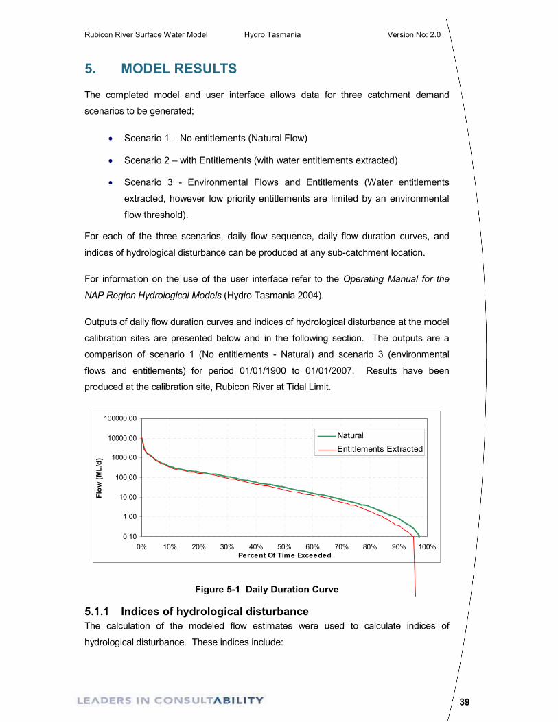
Outputs of daily flow duration curves and indices of hydrological disturbance at the model
calibration sites are presented below and in the following section. The outputs are a
comparison of scenario 1 (No entitlements - Natural) and scenario 3 (environmental
flows and entitlements) for period 01/01/1900 to 01/01/2007. Results have been
produced at the calibration site, Rubicon River at Tidal Limit.
0.10
1.00
10.00
100.00
1000.00
10000.00
100000.00
0% 10% 20% 30% 40% 50% 60% 70% 80% 90% 100%
Percent Of Time Exceeded
Flo
w (M
L/d
)
Natural
Entitlements Extracted
Figure 5-1 Daily Duration Curve
5.1.1 Indices of hydrological disturbance
The calculation of the modeled flow estimates were used to calculate indices of
hydrological disturbance. These indices include:
Rubicon River Surface Water Model Hydro Tasmania Version No: 2.0
40
• Index of Mean Annual Flow
• Index of Flow Duration Curve Difference
• Index of Seasonal Amplitude
• Index of Seasonal Periodicity
• Hydrological Disturbance Index
The indices were calculated using the formulas stated in the Natural Resource
Management (NRM) Monitoring and Evaluation Framework developed by SKM for the
Murray-Darling Basin (MDBC 08/04).
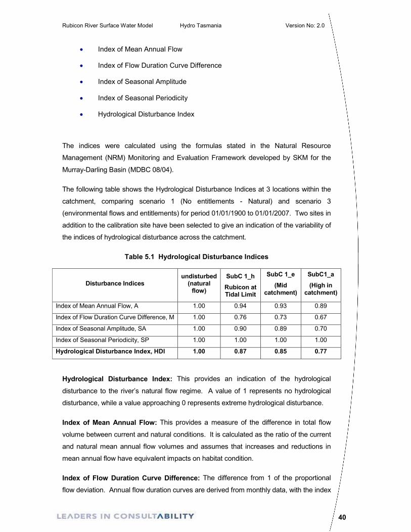
The following table shows the Hydrological Disturbance Indices at 3 locations within the
catchment, comparing scenario 1 (No entitlements - Natural) and scenario 3
(environmental flows and entitlements) for period 01/01/1900 to 01/01/2007. Two sites in
addition to the calibration site have been selected to give an indication of the variability of
the indices of hydrological disturbance across the catchment.
Table 5.1 Hydrological Disturbance Indices
Disturbance Indices undisturbed
(natural flow)
SubC 1_h
Rubicon at Tidal Limit
SubC 1_e
(Mid catchment)
SubC1_a
(High in catchment)
Index of Mean Annual Flow, A 1.00 0.94 0.93 0.89
Index of Flow Duration Curve Difference, M 1.00 0.76 0.73 0.67
Index of Seasonal Amplitude, SA 1.00 0.90 0.89 0.70
Index of Seasonal Periodicity, SP 1.00 1.00 1.00 1.00
Hydrological Disturbance Index, HDI 1.00 0.87 0.85 0.77
Hydrological Disturbance Index: This provides an indication of the hydrological
disturbance to the river’s natural flow regime. A value of 1 represents no hydrological
disturbance, while a value approaching 0 represents extreme hydrological disturbance.
Index of Mean Annual Flow: This provides a measure of the difference in total flow
volume between current and natural conditions. It is calculated as the ratio of the current
and natural mean annual flow volumes and assumes that increases and reductions in
mean annual flow have equivalent impacts on habitat condition.
Index of Flow Duration Curve Difference: The difference from 1 of the proportional
flow deviation. Annual flow duration curves are derived from monthly data, with the index
Rubicon River Surface Water Model Hydro Tasmania Version No: 2.0
41
being calculated over 100 percentile points. A measure of the overall difference between
current and natural monthly flow duration curves. All flow diverted would give a score of
0.
Index of Seasonal Amplitude: This index compares the difference in magnitude
between the yearly high and low flow events under current and natural conditions. It is
defined as the average of two current to natural ratios. Firstly, that of the highest monthly
flows, and secondly, that of the lowest monthly flows based on calendar month means.
Index of Seasonal Periodicity: This is a measure of the shift in the maximum flow
month and the minimum flow month between natural and current conditions. The
numerical value of the month with the highest mean monthly flow and the numerical
value of the month with the lowest mean monthly flow are calculated for both current and
natural conditions. Then the absolute difference between the maximum flow months and
the minimum flow months are calculated. The sum of these two values is then divided by
the number of months in a year to get a percentage of a year. This percentage is then
subtracted from 1 to give a value range between 0 and 1. For example a shift of 12
months would have an index of zero, a shift of 6 months would have an index of 0.5 and
no shift would have an index of 1.
Rubicon River Surface Water Model Hydro Tasmania Version No: 2.0
42
6. FLOOD FREQUENCY ANALYSIS
A flood frequency plot has been developed at the Rubicon at Tidal Limit (site 17200).
The plot shown below in Figure 6-1 consists of three traces:
1. Observed data. The annual maxima for this trace have been developed from
continuous measured data at the site giving a better representation of the flood
peak than the modelled daily average maxima. At the Rubicon at Tidal limit site
in total 39 annual maxima values were available for this flood frequency
analysis. The confidence limits on the plots represent the level of certainty of
this observed dataset.
2. Modelled data (Scenario 3 - Environmental Flows & Entitlements) – same
period as observed data. Note that the modelled annual maxima have been
determined from a daily average flow dataset and accordingly do not represent
the instantaneous flood maximum.
3. Modelled data (Scenario 3 - Environmental Flows & Entitlements) – whole
period of record. Note that the modelled annual maxima have been determined
from a daily average flow dataset and the period of record analysed is from
1900 to 2007.
The difference between flood peak frequency derived from recorded continuous flow
data and flood peak frequency derived from modelled daily average flow can be
obtained by comparing the first two traces as these relate to the same time period.
However, it should be noted that during the calibration process the highest priority was
to achieve the best volume match between modelled and observed. As a result, the
matching of flood peaks during calibration was of a lesser priority. Also the modelled
flood peaks are based on daily (total) rainfall and accordingly these lack the temporal
refinement to produce peaky outputs. That is, flood events are usually based on high
intensity rainfall and this is not accurately captured using models and rainfall run on a
daily time step.
These two factors do affect the accuracy of the modelled flood peaks used in the
development of this flood frequency curve.
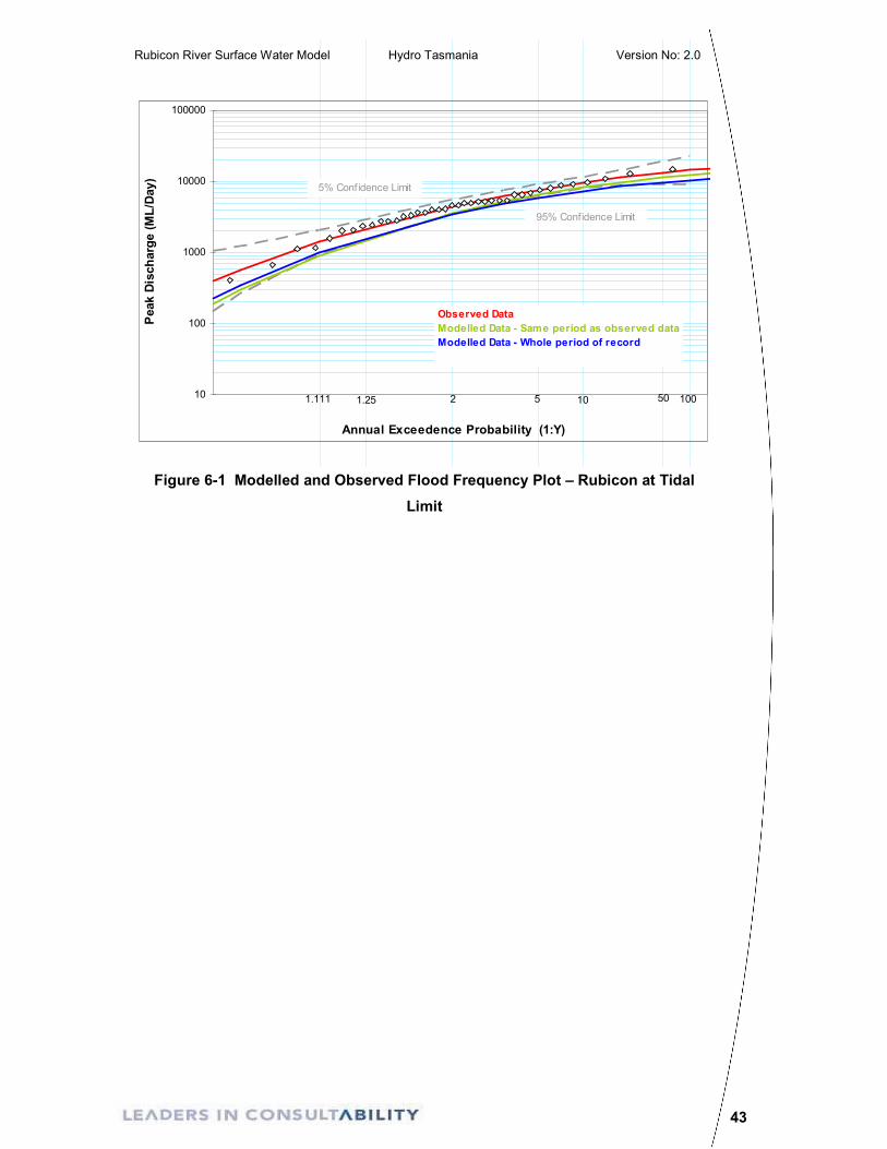
Rubicon River Surface Water Model Hydro Tasmania Version No: 2.0
43
21.25 5 5010 1001.11110
100
1000
10000
100000
Annual Exceedence Probability (1:Y)
Peak D
ischarg
e (M
L/D
ay)
95% Confidence Limit
5% Confidence Limit
Observed Data
Modelled Data - Same period as observed data
Modelled Data - Whole period of record
Figure 6-1 Modelled and Observed Flood Frequency Plot – Rubicon at Tidal
Limit
Rubicon River Surface Water Model Hydro Tasmania Version No: 2.0
44
7. REFERENCES
Boughton, W.C. and Chiew, F. (2003) Calibrations of the AWBM for use on Ungauged
Catchments
CatchmentSIM Homepage www.toolkit.net.au/catchsim/ , December 2006
QNRM Silo (Drill Data) Homepage www.nrm.qld.gov.au/silo , January 2005
SKM (2003) Estimating Available Water in Catchments in Catchments Using Sustainable
Diversion Limits. Farm Dam Surface Area and Volume relationship, report to DSE, Draft
B October 2003
Hydrology Theme Summary of Pilot Audit Technical Report – Sustainable Rivers Audit.
MDBC Publication 08/04.
National Land and Water Resources Audit (NLWRA) www.audit.ea.gov.au/anra/water/;
January 2005.
Hydro Tasmania internal report, (2004) South Esk River Catchment Above Macquarie
River, Impact of Water Entitlements on Water and Hydro Power Yield.
Hydro Tasmania, (2005), NAP Region Hydrological Model, North Esk Catchment.
Hydro Tasmania (2004). Operating Manual for the NAP region Hydrological Models.
Hydro Report 118783 – Report -015, 17 September 2004.
Neal B, Nathan RJ, Schreider S, & Jakeman AJ. 2002, Identifying the separate impact of
farm dams and land use changes on catchment yield. Aust J of Water Resources,
IEAust,; 5(2):165-176.
Parkyn R & Wilson D, (1997): Real-Time Modelling of the Tributary Inflows to ECNZ's
Waikato Storages. 24th Hydrology & Water Resources Symposium Proceedings
IEAust, Auckland NZ 1997.
State of the Environment Report, Tasmania, Volume 1 Conditions & Trends 1996. State
of Environment Unit, Lands Information Services, DELM.
SKM (2005) Development and Application of a Flow Stress Ranking Procedure, report
to Department of Sustainability and Environment, Victoria.
Rubicon River Surface Water Model Hydro Tasmania Version No: 2.0
45
Willis, M and Peterson, J. (2007) DPIW Surface Water Models - Leven & Gawler
catchment V2. Hydro Tasmania Consulting Report, Document no. WR 2007/001.
7.1 Personal Communications
Graham, B. Section Head, Ecohydrology, Water Assessment, DPIW. Oct 2007.
Rubicon River Surface Water Model Hydro Tasmania Version No: 2.0
46
8. GLOSSARY
Coefficient of determination (R2): One of the most common measures of comparison
between two sets of data is the coefficient of determination (R2). If two data sets are
defined as x and y, R2 is the variance in y attributable to the variance in x. A high R2
value indicates that x and y vary together – that is, the two data sets have a good
correlation
High priority entitlements: Water entitlements with an assigned Surety 1 to 3.
Low priority entitlements: Water entitlements with an assigned Surety 4 to 8.
Modelled – No entitlements (Natural): The TimeStudio surface water model run in a
natural state. That is, all references to water entitlements have been set to zero.
Additionally any man made structures such as dams, power stations and diversions
have been omitted and the modelled flow is routed, uncontrolled through the
catchment. This is also referred to as Scenario 1.
Modelled – No entitlements (Modified): The TimeStudio surface water model run
with no water entitlements extracted. That is, all references to water entitlements have
been set to zero. Where human structures are identified that significantly affect the flow
regime, such as large dams, power stations and diversions, the TimeStudio model
contains custom code to estimate the flow effect on the downstream subareas. This
custom code takes effect from the completion date of the structure. Where there are no
significant human structures in the catchment or the model is run before the completion
of these structures this model will produce the same output as “Modelled – No
entitlements (Natural)”. This option is not available within the user interface and is one
of several inputs used to derive a modelled flow specifically for calibration purposes. It
is also referred to as MNEM in Section 4.4.
Modelled – with entitlements (extracted): The TimeStudio surface water model with
water entitlements removed from the catchment flow. Where human structures are
identified within a catchment that significantly affect the flow regime, such as large
dams, power stations and diversions, the TimeStudio model contains custom code to
estimate the flow effect on the downstream sub-catchments. This custom code takes
effect from the completion date of the structure. This is also referred to as Scenario 2.
Rubicon River Surface Water Model Hydro Tasmania Version No: 2.0
47
Modelled – environmental flows and entitlements (extracted): The
TimeStudiosurface water model with water entitlements removed. However, low priority
entitlements are only removed when sub-catchment flow exceeds a specified
environmental threshold. Where man made structures are identified within a
catchment, such as dams, power stations and diversions the TimeStudio model
contains code to estimate the flow effect on the downstream subcatchments,
commencing on the completion date of the structure. This is also referred to as
Scenario 3.
Time Period Reduction Factor (TPRF): A reduction factor applied to current levels of
water extracted from a catchment. The TPRF was applied to satisfy the assumption
that the amount of water extracted from Tasmanian catchments (e.g. for agriculture)
has increased over time. The TPRF was calculated by a method developed in the
Tasmanian State of the Environment report. This states that water demand has
increased by an average of 6% annually over the last 4 decades. This factor is applied
to current water entitlements to provide a simple estimate of water entitlements
historically. However, following discussions with DPIW the TPRF was capped at 50%
of the current extractions if the mid year of the calibration period was earlier than 1995.
Water entitlements: This refers generally to the potential water extraction from the
catchment. Included are licensed extractions documented in WIMS (July 2007)
estimates of additional unlicensed extractions and estimates of unlicensed farm dams.
Unless specified otherwise, Hydro Tasmania dams and diversions are not included.
WIMS (July 2007): The Department Primary Industries and Water, Water Information
Management System, updated to July 2007.
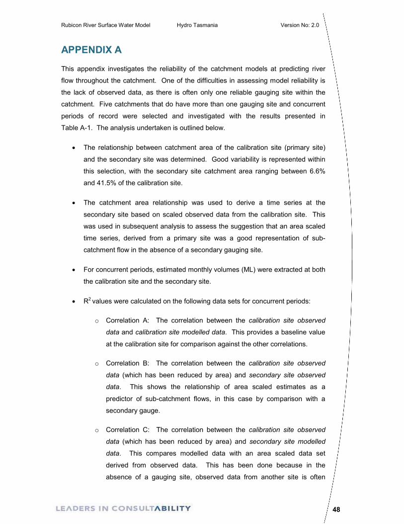
Rubicon River Surface Water Model Hydro Tasmania Version No: 2.0
48
APPENDIX A
This appendix investigates the reliability of the catchment models at predicting river
flow throughout the catchment. One of the difficulties in assessing model reliability is
the lack of observed data, as there is often only one reliable gauging site within the
catchment. Five catchments that do have more than one gauging site and concurrent
periods of record were selected and investigated with the results presented in
Table A-1. The analysis undertaken is outlined below.
• The relationship between catchment area of the calibration site (primary site)
and the secondary site was determined. Good variability is represented within
this selection, with the secondary site catchment area ranging between 6.6%
and 41.5% of the calibration site.
• The catchment area relationship was used to derive a time series at the
secondary site based on scaled observed data from the calibration site. This
was used in subsequent analysis to assess the suggestion that an area scaled
time series, derived from a primary site was a good representation of sub-
catchment flow in the absence of a secondary gauging site.
• For concurrent periods, estimated monthly volumes (ML) were extracted at both
the calibration site and the secondary site.
• R2 values were calculated on the following data sets for concurrent periods:
o Correlation A: The correlation between the calibration site observed
data and calibration site modelled data. This provides a baseline value
at the calibration site for comparison against the other correlations.
o Correlation B: The correlation between the calibration site observed
data (which has been reduced by area) and secondary site observed
data. This shows the relationship of area scaled estimates as a
predictor of sub-catchment flows, in this case by comparison with a
secondary gauge.
o Correlation C: The correlation between the calibration site observed
data (which has been reduced by area) and secondary site modelled
data. This compares modelled data with an area scaled data set
derived from observed data. This has been done because in the
absence of a gauging site, observed data from another site is often
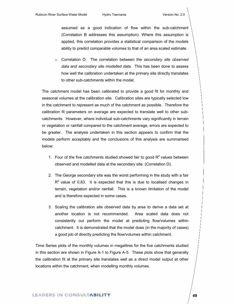
Rubicon River Surface Water Model Hydro Tasmania Version No: 2.0
49
assumed as a good indication of flow within the sub-catchment
(Correlation B addresses this assumption). Where this assumption is
applied, this correlation provides a statistical comparison of the models
ability to predict comparable volumes to that of an area scaled estimate.
o Correlation D: The correlation between the secondary site observed
data and secondary site modelled data. This has been done to assess
how well the calibration undertaken at the primary site directly translates
to other sub-catchments within the model.
The catchment model has been calibrated to provide a good fit for monthly and
seasonal volumes at the calibration site. Calibration sites are typically selected low
in the catchment to represent as much of the catchment as possible. Therefore the
calibration fit parameters on average are expected to translate well to other sub-
catchments. However, where individual sub-catchments vary significantly in terrain
or vegetation or rainfall compared to the catchment average, errors are expected to
be greater. The analysis undertaken in this section appears to confirm that the
models perform acceptably and the conclusions of this analysis are summarised
below:
1. Four of the five catchments studied showed fair to good R2 values between
observed and modelled data at the secondary site. (Correlation D).
2. The George secondary site was the worst performing in the study with a fair
R2 value of 0.83. It is expected that this is due to localised changes in
terrain, vegetation and/or rainfall. This is a known limitation of the model
and is therefore expected in some cases.
3. Scaling the calibration site observed data by area to derive a data set at
another location is not recommended. Area scaled data does not
consistently out perform the model at predicting flow/volumes within
catchment. It is demonstrated that the model does (in the majority of cases)
a good job of directly predicting the flow/volumes within catchment.
Time Series plots of the monthly volumes in megalitres for the five catchments studied
in this section are shown in Figure A-1 to Figure A-5. These plots show that generally
the calibration fit at the primary site translates well as a direct model output at other
locations within the catchment, when modelling monthly volumes.
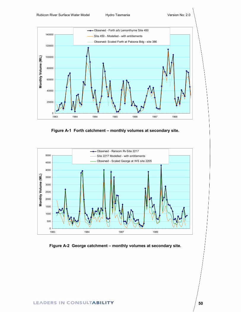
Rubicon River Surface Water Model Hydro Tasmania Version No: 2.0
50
0
20000
40000
60000
80000
100000
120000
140000
1963 1964 1964 1965 1966 1967 1968
Month
ly V
olu
me (M
L)
Observed - Forth a/b Lemonthyme Site 450
Site 450 - Modelled - with entitlements
Observed- Scaled Forth at Paloona Bdg - site 386
Figure A-1 Forth catchment – monthly volumes at secondary site.
0
500
1000
1500
2000
2500
3000
3500
4000
4500
5000
1983 1984 1987 1989
Month
ly V
olu
me (M
L)
Observed - Ransom Rv Site 2217
Site 2217 Modelled - with entitlements
Observed - Scaled George at WS site 2205
Figure A-2 George catchment – monthly volumes at secondary site.
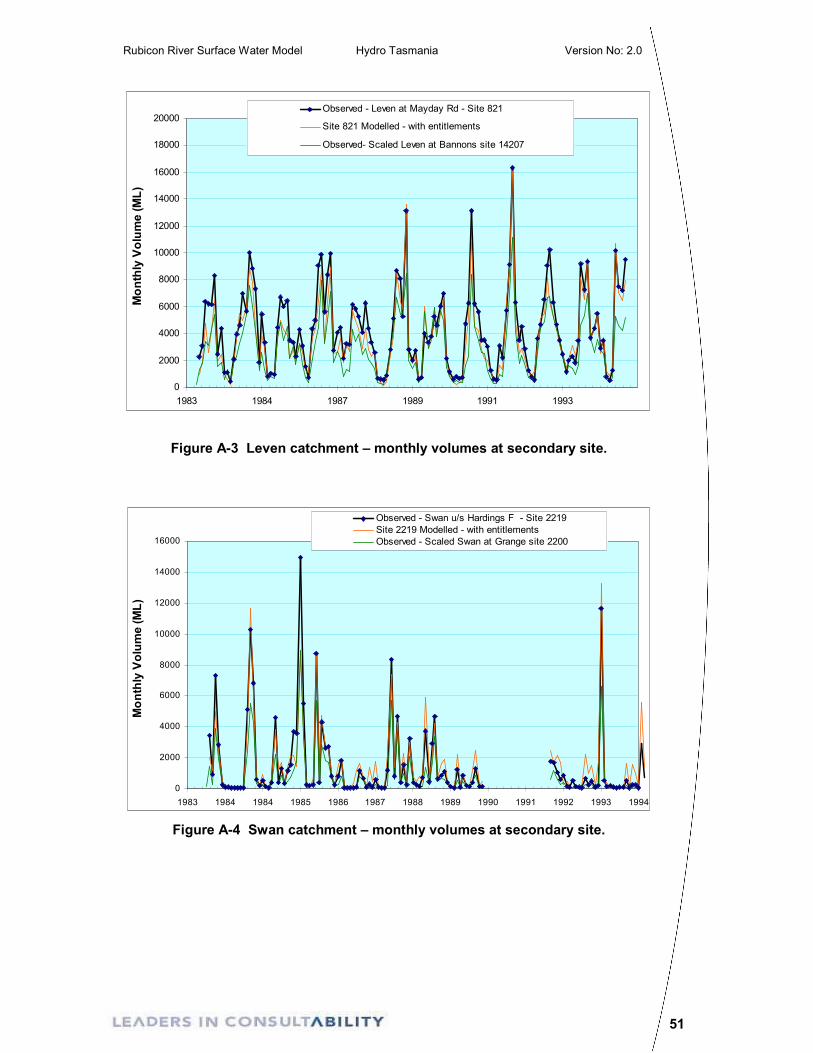
Rubicon River Surface Water Model Hydro Tasmania Version No: 2.0
51
0
2000
4000
6000
8000
10000
12000
14000
16000
18000
20000
1983 1984 1987 1989 1991 1993
Month
ly V
olu
me (M
L)
Observed - Leven at Mayday Rd - Site 821
Site 821 Modelled - with entitlements
Observed- Scaled Leven at Bannons site 14207
Figure A-3 Leven catchment – monthly volumes at secondary site.
0
2000
4000
6000
8000
10000
12000
14000
16000
1983 1984 1984 1985 1986 1987 1988 1989 1990 1991 1992 1993 1994
Month
ly V
olu
me (M
L)
Observed - Swan u/s Hardings F - Site 2219
Site 2219 Modelled - with entitlements
Observed - Scaled Swan at Grange site 2200
Figure A-4 Swan catchment – monthly volumes at secondary site.
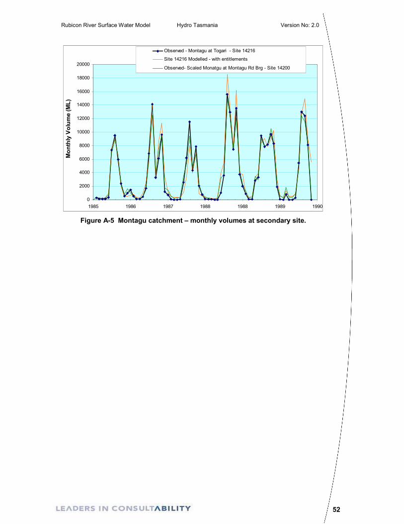
Rubicon River Surface Water Model Hydro Tasmania Version No: 2.0
52
0
2000
4000
6000
8000
10000
12000
14000
16000
18000
20000
1985 1986 1987 1988 1988 1989 1990
Month
ly V
olu
me (M
L)
Observed - Montagu at Togari - Site 14216
Site 14216 Modelled - with entitlements
Observed- Scaled Monatgu at Montagu Rd Brg - Site 14200
Figure A-5 Montagu catchment – monthly volumes at secondary site.
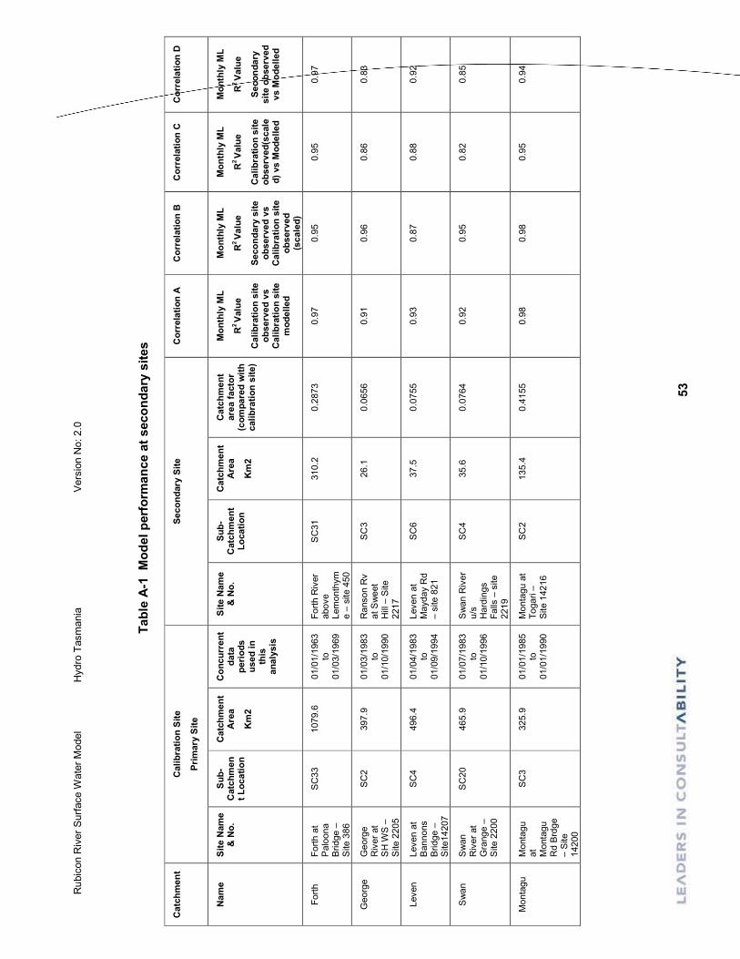
Rubicon River Surface Water Model Hydro Tasmania
Version No: 2.0
53
Table
A-1
M
odel perf
orm
ance a
t secondary
sites
Catc
hm
ent
Calibra
tion S
ite
Prim
ary
Site
Secondary
Site
Corr
ela
tion A
C
orr
ela
tion B
C
orr
ela
tion C
C
orr
ela
tion D
Nam
e
Site N
am
e
& N
o.
Sub-
Catc
hm
en
t Location
Catc
hm
ent
Are
a
Km
2
Concurr
ent
data
peri
ods
used in
this
analy
sis
Site N
am
e
& N
o.
Sub-
Catc
hm
ent
Location
Catc
hm
ent
Are
a
Km
2
Catc
hm
ent
are
a facto
r (c
om
pare
d w
ith
calibra
tion s
ite)
Month
ly M
L
R2 V
alu
e
Calibra
tion s
ite
observ
ed v
s
Calibra
tion s
ite
modelled
Month
ly M
L
R2 V
alu
e
Secondary
site
observ
ed v
s
Calibra
tion s
ite
observ
ed
(scale
d)
Month
ly M
L
R2 V
alu
e
Calibra
tion s
ite
observ
ed(s
cale
d) vs M
odelled
Month
ly M
L
R2 V
alu
e
Secondary
site o
bserv
ed
vs M
odelled
Forth
Forth at
Paloona
Bridge –
Site 386
SC33
1079.6
01/01/1963
to
01/03/1969
Forth River
above
Lemonthym
e – site 450
SC31
310.2
0.2873
0.97
0.95
0.95
0.97
George
George
River at
SH WS –
Site 2205
SC2
397.9
01/03/1983
to
01/10/1990
Ranson Rv
at Sweet
Hill – Site
2217
SC3
26.1
0.0656
0.91
0.96
0.86
0.83
Leven
Leven at
Bannons
Bridge –
Site14207
SC4
496.4
01/04/1983
to
01/09/1994
Leven at
Mayday Rd
– site 821
SC6
37.5
0.0755
0.93
0.87
0.88
0.92
Swan
Swan
River at
Grange –
Site 2200
SC20
465.9
01/07/1983
to
01/10/1996
Swan River
u/s
Hardings
Falls – site
2219
SC4
35.6
0.0764
0.92
0.95
0.82
0.85
Montagu
Montagu
at Montagu
Rd Brdge
– Site
14200
SC3
325.9
01/01/1985
to
01/01/1990
Montagu at
Togari –
Site 14216
SC2
135.4
0.4155
0.98
0.98
0.95
0.94