Dr Martin Hendry,School of Physics and AstronomyUniversity of Glasgow, UK

Astronomical Data

Analysis I

11 lectures, beginning autumn 2010

5. Fourier Methods

As we remarked in Section 1, a lot of astronomical data is

collected or processed as Fourier components.

In this section we briefly discuss the mathematics of Fourier

series and Fourier transforms. Some of these methods will be

applied to astronomical problems in ADA II.

5.1 Fourier Series

Any ‘well-behaved’ function can be

expanded in terms of an infinite sum of sines

and cosines. The expansion takes the form:

Joseph Fourier(1768-1830)

)(xf

1 1

021 sincos)(

n nnn nxbnxaaxf (5.1)

The Fourier coefficients are given by the formulae:

These formulae follow from the orthogonality properties of sin and cos:

dxxfa )(

10 (5.2)

nxdxxfan cos)(

1

nxdxxfbn sin)(

1

(5.3)

(5.4)

mnnxdxmx

sinsin mnnxdxmx

coscos

0cossin nxdxmx

Some examples from Mathworld, approximating functions with a finite number of Fourier series terms

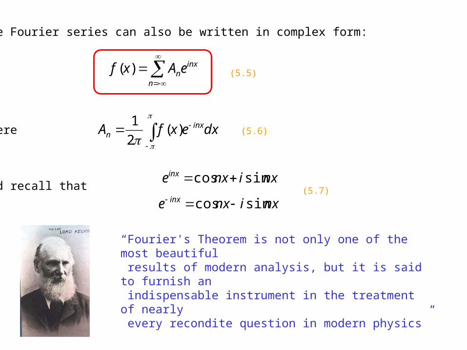
“Fourier's Theorem is not only one of the most beautiful results of modern analysis, but it is said to furnish an indispensable instrument in the treatment of nearly every recondite question in modern physics”

The Fourier series can also be written in complex form:

where

and recall that

n

inxneAxf )( (5.5)

dxexfA inx

n )(2

1(5.6)

nxinxeinx sincos

nxinxe inx sincos (5.7)

The Fourier transform can be thought of simply as extending the

idea of a Fourier series from an infinite sum over discrete, integer

Fourier modes to an infinite integral over continuous Fourier modes.

Consider, for example, a physical process that is varying in the time

domain,

i.e. it is described by some function of time .

Alternatively we can describe the physical process in the frequency

domain by defining the Fourier Transform function .

It is useful to think of and as two different

representations of the same function; the information they convey

about the underlying physical process should be equivalent.

)(th

5.2 Fourier Transform: Basic Definition

)( fH

)(th )( fH

We define the Fourier transform as

and the corresponding inverse Fourier transform as

If time is measured in seconds then frequency is measured in cycles

per second, or Hertz.

dtethfH tif2)()( (5.8)

dfefHth tif2)()( (5.9)

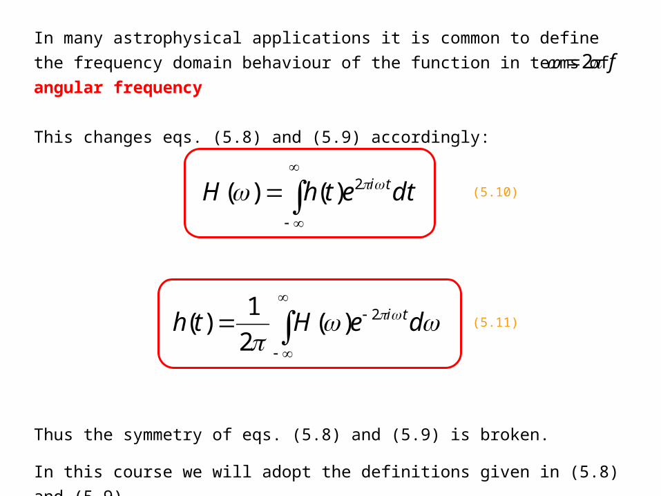
In many astrophysical applications it is common to define the

frequency domain behaviour of the function in terms of angular

frequency

This changes eqs. (5.8) and (5.9) accordingly:

Thus the symmetry of eqs. (5.8) and (5.9) is broken.

In this course we will adopt the definitions given in (5.8) and (5.9)

f 2

dtethH ti 2)()( (5.10)

deHth ti2)(2

1)( (5.11)

5.3 Fourier Transform: Further properties

The FT is a linear operation:

(1) the FT of the sum of two functions is equal to the sum of their FTs

(2) the FT of a constant times a function is equal to the constant times

the FT of the function.

If the time domain function is a real function, then its FT is

complex.

However, more generally we can consider the case where is also

a

complex function – i.e. we can write

may also possess certain symmetries: even function

odd function

)(th

)(th

)()()( tihthth IR (5.12)

Real partImaginary part

)(th )()( thth

)()( thth

The following properties then hold:

Note that in the above table a star (*) denotes the complex

conjugate, i.e. if z = x + i y then z* = x − i y

See Numerical Recipes, Section 12.0

For convenience we will denote the FT pair by

It is then straightforward to show that

)()( fHth

)(1

)( afHa

ath (5.13) “time scaling”

)()(1

fbHbthb

(5.14) “frequency scaling”

020 )()( tfiefHtth (5.15)

“frequency scaling”

“time shifting”

(5.16))()( 02 0 ffHeth tfi

Suppose we have two functions and

Their convolution is defined as

We can prove the Convolution Theorem

i.e. the FT of the convolution of the two functions is equal to the product of their individual FTs.

Also their correlation, which is also a function of t , is defined as

)(tg )(th

dssthsgthg )()()( (5.17)

)()()( fHfGthg (5.18)

dsshtsghg )()(),(Corr (5.19)

Known as the lag

We can prove the Correlation Theorem

i.e. the FT of the first time domain function, multiplied by the complex conjugate of the FT of the second time domain function, is equal to the FT of their correlation.

The correlation of a function with itself is called the auto-correlation

In this case

The function is known as the power spectral density,

or (more loosely) as the power spectrum.

Hence, the power spectrum is equal to the Fourier Transform of the

auto-correlation function for the time domain function

)()(),(Corr fHfGhg

(5.21)

(5.20)

2)(),(Corr fGgg

2)( fG

)(tg

5.4 The power spectral density

The power spectral density is analogous to the pdf we defined in

previous sections.

In order to know how much power is contained in a given interval of

frequency, we need to integrate the power spectral density over

that interval.

The total power in a signal is the same, regardless of whether we

measure it in the time domain or the frequency domain:

- -

22PowerTotal dfH(f)dth(t) (5.22)

Parseval’s Theorem

We can, therefore, think of moving between the time and frequency domain as analogous to the change of variables we employed for pdfs in Section 4

Often we will want to know how much power is contained in a

frequency interval without distinguishing between positive and

negative values.

In this case we define the one-sided power spectral density:

And

When is a real function

With the proper normalisation, the total power (i.e. the integrated

area under the relevant curve) is the same regardless of whether

we are working with the time domain signal, the power spectral

density or the one-sided power spectral density.

ffHfHfPh 0)()()(22

(5.23)

0

)(PowerTotal dffPh (5.24)

)(th 2)(2)( fHfPh (5.25)

From Numerical Recipes,Chapter 12.0

Time domain

One-sided PSD

Two-sided PSD

const.)( th

t

)(th

)0()( DfH

f

)( fH

0 0

Dirac Delta function

tfieth 02)(

t

)(th

0

Imaginary partReal part

)()( 0D fffH

f

)( fH

0

(1)

(2)

5.5 Examples

xy sinc

x

1y

xatzero1stxatzero1st

otherwise0

for1)( 2

121 t

th

t

)(th

0

(3)

)(sinc)( ffH

f

)( fH

0

Imaginary part = 0

The sinc function occurs frequently in many areas of astrophysics

The function has a maximum at and the zeros occur at

for positive integer m

x

xx

sinsinc

0xmx

1/2 t0

1

-1/2

(4) )()( tth

f0

1

)(sinc)( 2 ffH

(5)

Real part

Imaginary part

ateth )(

2222

2

222

2

4

2)(Im

4)( Re

fa

fafH

fa

afH

)( fH

)( fH

t

222

2

4)( Re

fa

afH

This function is a Lorentzian

and is commonly modelled as the

shape of spectral line profiles in

astronomy.

One can also show that the

Power Spectrum corresponding

to this FT is also a Lorentzian.

(See examples).

)( fH

f

i.e. the FT of a Gaussian function in the time domain is also a

Gaussian in the frequency domain.

The broader the Gaussian is in the time domain, then the narrower

the Gaussian FT in the frequency domain, and vice versa.

(6) 2exp)( atth

t0

f0

222 /exp)( affH

Although we have discussed FTs so far in the context of a

continuous, analytic function, , in many practical situations we

must work instead with observational data which are sampled at a

discrete set of times.

Suppose that we sample in total times at evenly

spaced time intervals , i.e. (for even)

[ If is non-zero over only a finite interval of time, then we

suppose that the sampled points contain this interval. Or if

has an infinite range, then we at least suppose that the

sampled points cover a sufficient range to be representative of the

behaviour of ].

5.6 Discrete Fourier Transforms

)(th

)(th

(5.26)2,...,0,...,2, NNkktk )( kk thh where

1N

)(th

1N )(th

)(th

N

We therefore approximate eq. (5.8) as

Since we are sampling at discrete timesteps, in view of

the symmetry of the FT and inverse FT it makes sense also to

compute

only at a set of discrete frequencies:

(The frequency is known as the Nyquist (critical)

frequency and it is a very important value. We discuss its

significance in Section 6).

2

2

22)()(Nk

Nk

tifk

tif kehdtethfH (5.27)

)(th 1N)( fH

1N

2,...,0,...,2, NNnN

nfn

(5.28)

21cf

Then

Note that

Hence, in eq. (5.29) there are only independent values.

Also, note that

So we can re-define eq. (5.29) as:

n

N

k

Nnkikn HehfH

1

0

/2)(

nini ee (5.30)

N

NkNniNnkiniNnki eee /)(2/22/2

(5.31)

2

2

/22

2

2)(Nk

Nk

Nnkik

Nk

Nk

tifkn ehehfH kn

(5.29)

Discrete Fourier Transform of the kh

The discrete inverse FT, which recovers the set of from the

set of

is

Parseval’s theorem for discrete FTs takes the form

There are also discrete analogues to the convolution and correlation

theorems.

s'khs'nH

1

0

/21 N

k

Nnkink eH

Nh

(5.32)

1

0

21

0

2 1 N

nn

N

kk H

Nh (5.33)

Consider again the formula for the discrete FT. We can write it as

This is a matrix equation: we compute the vector of

by multiplying the matrix by the vector of

.

In general, this requires of order multiplications (and the

may be complex numbers).

e.g. suppose . Even if a computer can

perform (say) 1 billion multiplications per second, it would still

require more than 115 days to calculate the FT.

5.7 Fast Fourier Transforms

(5.34)

1

0

1

0

/2N

kk

nkN

kk

Nnkin hWheH

s'kh)1( N s'nH

)( NN nkW )1( N

2N s'kh

1628 1010 NN

Fortunately, there is a way around this problem.

Suppose (as we assumed before) is an even number. Then we can

write

where

So we have turned an FT with points into the weighted sum of two

FTs with points. This would reduce our computing time by a

factor of two.

N

12/

012

/)12(212/

02

/)2(21

0

/2N

jj

NnjiN

jj

NnjiN

kk

Nnkin heheheH

(5.35)

Even values of k Odd values of k

1

012

/21

02

/2M

jj

MnjinM

jj

Mnji heWhe

2/NM

N2/N

(5.36)

Why stop there, however?...

If is also even, we can repeat the process and re-write the FTs of

length as the weighted sum of two FTs of length .

If is a power of two (e.g. 1024, 2048, 1048576 etc) then we

can repeat iteratively the process of splitting each longer FT into two

FTs half as long.

The final step in this iteration consists of computing FTs of length unity:

i.e. the FT of each discretely sampled data value is just the data value

itself.

MM 2/M

……

N

00

020 hheH

kk

ki

(5.37)

This iterative process converts multiplications into

operations.

So our operations are reduced to about

operations.

Instead of 100 days of CPU time, we can perform the

FT in less than 3 seconds.

The Fast Fourier Transform (FFT) has revolutionised our ability to tackle

problems in Fourier analysis on a desktop PC which would otherwise be

impractical, even on the largest supercomputers.

)( 2NO)log( 2 NNO

This notation means ‘of the order of’

16109107.2