draft: analysis and modelling of entropy modes in a realistic aeronautical gas...

Proceedings of ASME Turbo Expo 2013GT2013

June 3-7, 2013, San Antonio, Texas, USA

GT2013-94224

DRAFT: ANALYSIS AND MODELLING OF ENTROPY MODES IN A REALISTICAERONAUTICAL GAS TURBINE

Emmanuel Motheau ∗

Safran Snecma and CERFACS42 av. Gaspard Coriolis

31057 Toulouse - FranceEmail: [email protected]

Franck NicoudCNRS UMR 5149

University Montpellier II34095 Montpellier - France

Email : [email protected]

Yoann MerySafran Snecma

Rond Point Rene Ravaud77550 Moissy Cramayel - FranceEmail : [email protected]

Thierry PoinsotCNRS - Institut de mecanique des fluides

1 Allee du Professeur Camille Soula31000 Toulouse - France

Email : [email protected]

ABSTRACTA combustion instability in a combustor typical of aero-

engines is analyzed and modeled thanks to a low order Helmholtzsolver. A Dynamic Mode Decomposition (DMD) is first appliedto the Large Eddy Simulation (LES) database. The mode withthe highest amplitude shares the same frequency of oscillationas the experiment (approx. 350 Hz) and it shows the presenceof large entropy spots generated within the combustion cham-ber and convected down to the exit nozzle. The lowest purelyacoustic mode being in the range 650-700 Hz, it is postulatedthat the instability observed around 350 Hz stems from a mixedentropy/acoustic mode where the acoustic generation associatedwith the entropy spots being convected throughout the chokednozzle plays a key role. A Delayed Entropy Coupled BoundaryCondition is then derived in order to account for this interactionin the framework of a Helmholtz solver where the baseline flowis assumed at rest. When fed with appropriate transfer functionsto model the entropy generation and convection from the flameto the exit, the Helmholtz solver proves able to predict the pres-ence of an unstable mode around 350 Hz, in agreement with boththe LES and the experiments. This finding supports the idea that

∗Address all correspondence to this author.

the instability observed in the combustor is indeed driven by theentropy/acoustic coupling.

NOMENCLATUREp Static pressurec Sound speedω Angular frequencyγ Ratio of the specific heatsq Heat release rate per unit volumeg fluctuating part of quantity gLES Large Eddy SimulationsLEE Linearized Euler EquationsDMD Dynamic Mode DecompositionDECBC Delayed Entropy Coupled Boundary ConditionTres Flow-through timeρ DensityJ Total stagnation enthalpym Mass-flow rateu Fluid velocityM Mach numberk Wave number

1 Copyright c© 2013 by ASME

g0 Subscript for mean quantity of gs EntropyCp Heat capacity per mass unit at fixed pressureτ Convection time delaynre f Unitary reference vectorure f Velocity at reference pointG Gain of the transfer functionZ ImpedanceZp,u Impedance defined with state variables p and uZJ,m Impedance defined with state variables J and mZ0 Impedance imposed at the edge of the zero Mach number

domainZM Impedance computed at the edge of the LEE domain

IntroductionIt has been long known that combustion instabilities in in-

dustrial systems can lead to high amplitude oscillations of allphysical quantities (pressure, velocities, temperature, etc.). Aclassical mechanism for combustion instability is a construc-tive coupling between acoustic waves and the unsteady com-bustion that arises when pressure and heat release fluctuationsare in phase [1, 2]. Another mechanism that may also supportself-sustained instabilities relies on the acoustic perturbationsinduced by entropy spots (temperature and/or mixture hetero-geneities say) being generated in the flame region and evacuatedthrough the downstream nozzle [3, 4]. This latter mechanismis particularly relevant to (high speed) reacting flows where theflow through time is small and turbulent mixing cannot signifi-cantly reduce the amplitude of the entropy spots being convectedfrom the flame region to combustor exit.

Several recent studies have shown that the Large Eddy Simu-lation (LES) approach is a powerful tool for studying the dynam-ics of turbulent flames and their interactions with the acousticwaves [5, 6]. However, these simulations are very CPU demand-ing and faster tools are required in the design process of newburners. A natural approach is to characterize the stable/unstablemodes in the frequency domain. An approximate linear waveequation for the amplitude p(~x) of the pressure perturbationsp(~x, t) = p(~x)exp(− jωt) in reacting flows may be derived fromthe Navier-Stokes equations [7] and reads:

∇ ·(c2

0∇ p)+ω

2 p = jω(γ −1)q (1)

where q(~x) is the amplitude of the unsteady heat release q(~x, t) =q(~x)exp(− jωt), c0 is the speed of sound, and ω is the complexangular frequency. In order to close the problem, the flame is of-ten modeled as a purely acoustic element thanks to a n− τ typeof model [8] which essentially relates the unsteady heat releaseto acoustic quantities at reference locations; Eq. (1) then corre-sponds to a non-linear eigenvalue problem which can be solvedby using appropriate algorithms [9].

Eq. (1) relies on the so-called zero Mach number assump-tion stating that the mean velocity is very small compared tothe speed of sound. A recent study suggests that the domainof validity of the zero mean flow assumption might be rathersmall [10]. One reason for this is that Eq. (1) does not supportentropy waves. Thus the acoustic generation due to the entropyspot being accelerated in the nozzle/turbine located downstreamof the combustion chamber is not accounted for. Since the pro-duction of sound by acceleration of entropy fluctuations is a keyphenomenon when dealing with combustion noise [11, 12], ne-glecting this acoustic source when studying thermoacoustic in-stabilities is highly questionable. Note also that mixed modesmay exist that rely on a convective path and acoustic feedbackwhen the baseline flow is not at rest [3], and that cannot be cap-tured when using Eq. (1).

Nevertheless, this somewhat restrictive assumption is neces-sary to derive a wave equation for the thermoacoustic perturba-tions superimposed to a non isentropic baseline flow, the alterna-tive being to use the complete set of Linearized Euler Equations(LEE) [10]. Unfortunately, this would make the computationaleffort needed to compute the thermoacoustic modes significantlylarger (five coupled equations being solved for) than what is re-quired when dealing with Eq. (1). Being able to partly accountfor the non zero Mach number effects without relying on theLEEs is therefore highly desirable. The objectives of this paperare then as follows:

• analyze fully nonlinear large-eddy simulation data to test forthe presence of mixed modes in a realistic combustion cham-ber;

• develop and validate a methodology to mimic the mean floweffects within the zero Mach number framework (Eq. 1);

• apply the method to a 3D industrial combustor whereentropy-acoustic coupling is included in the Helmholtzsolver framework.

First, the industrial configuration and associated instabil-ity are presented in Section 1; a Dynamic Mode Decomposi-tion (DMD) is applied to the LES results in order to investigatethe presence of an entropy-acoustic coupling. A proper formal-ism is then introduced in Section 2 in order to account for theentropy-acoustic coupling within the zero Mach number frame-work. The underlying Delayed Entropy Coupled Boundary Con-dition (DECBC) is also validated in this section by consideringan academic quasi-1D combustor mounted on a nozzle. Finally,results from a zero Mach number Helmholtz solver with andwithout the DECBC approach are presented in Section 3 to il-lustrate the benefit of the method.


FIGURE 1. Description of the configuration of interest. One sectorof the azimuthal SAFRAN combustor is represented.

1 Description of the combustor and analysis1.1 Geometry

The case considered in this study is a combustor developedby the SAFRAN Group for aero-engine applications. The mainparts are displayed in Figure 1 which shows the combustionchamber and the casing with primary and dilution holes. Theair inlet connected to the upstream compressor is also displayed.Note that the downstream high pressure distributor which con-nects the combustor to the turbine is modelled by a chocked noz-zle with equivalent cross section area. For chocked conditions,this ensures that the chamber sees an acoustic environment closeto the actual one. The fuel line is also visible, as well as a cutof the swirled injector used to mix fuel and air and to generatethe recirculation zone which stabilizes the flame. In the actualsituation, several injectors are mounted all around the azimuthalcombustion chamber although only one sector with one injec-tor is displayed in the figure. For confidentiality concerns, someparts of the geometry are not displayed in Figures 1, 2, 3 and 6.

1.2 DMD analysis of the LES dataExperiments were performed by SAFRAN on the configu-

ration described in section 1.1. Under certain operating condi-tions, the configuration becomes unstable at approximately 350Hz. To analyze this instability, large eddy simulations (LES)were performed at CERFACS and SAFRAN. For this purpose,the general AVBP [13] code developed at CERFACS and IFPEnergies Nouvelles was used. It is based on a cell-vertex formu-lation and embeds a set of finite element / finite volume schemesfor unstructured meshes. In the present study an implementa-tion of the Lax-Wendroff scheme (2nd order in time and space)was retained. Two regimes were computed by LES, correspond-ing to the two operating conditions investigated experimentallyat SAFRAN: one which contains an instability at 350 Hz andone which shows no instability. Although not discussed in thispaper, the LES was able to distinguish these two regimes verynicely, displaying a stable turbulent flame for the latter regime

FIGURE 2. Typical snapshot from the LES of the SAFRAN combus-tor and time evolution of pressure within the chamber.

and an unstable mode close to 330 Hz for the former. Theseflows were computed over a 4.5 million elements mesh withthe static Smagorinsky subgrid scale model whereas turbulentcombustion was represented with the Dynamic Thickened FlameModel [14]. A simple two-step kinetic scheme was used to repre-sent the kerosene-air flame in the combustor [15]. The boundaryconditions are imposed through the NSCBC formulation [16] soas to prevent spurious acoustic reflections. Note that as the noz-zle is chocked, the physics inside the combustion chamber de-pends only upon the sonic throat which imposes the effectiveoutlet state. Figure 2 displays a typical snapshot of the LESwhere the complex 3D flame structure can be seen on top of thetemperature field. A pressure signal at a probe within the com-bustion chamber demonstrates the presence of a thermoacousticinstability at approx. 350 Hz. The amplitude of the limit cycle isquite large and may be explained by the fact that some acousticdampers such as perforated liners were not included in the com-putations. However, this result is in the range of pressure fluctu-ations amplitudes measured in the experiments (∼ 8.104 Pa peakto peak). Note also the the amplitude was found robust to theshape of the nozzle used to mimic the high pressure distributor.

Dynamic Mode Decomposition (DMD) was applied to theLES data in order to better understand the nature of the insta-


FIGURE 3. Fluctuating pressure (left) and temperature (right) from the DMD mode at 331 Hz. From top to bottom, the four rows correspond tophases 0, π/2, π and 3π/2.

bility illustrated in Figure 2. For this purpose, 250 snapshotswere recorded over a time range corresponding to approx. 13cycles characteristics of the instability phenomena, thus leadingto a sampling of 20 snapshots by period. This amount of datais sufficient for the DMD to breakdown the reactive turbulentflow into dynamically relevant structures with periodic evolution

over time [17]. Note that the input vectors for the DMD algo-rithm were built from the nodal values of pressure, static tem-perature and reaction rate at each grid point of the mesh usedfor the LES. The fluctuating pressure and temperature fields re-constructed from the DMD mode with the highest amplitude aredisplayed in Figure 3. Note that this mode oscillates at 331 Hz,


in good agreement with the experimental data. The four phasesdisplayed in Figure 3 support the idea that the unstable mode ofinterest relies, at least partly, on an entropy-acoustic coupling. Atphase 0, the pressure is low everywhere within the combustionchamber and a pocket of cold gas is present downstream of theprimary reaction zone, roughly at the middle of the combustionchamber. At phase π/2, this pocket is convected downstreamand the unsteady pressure in the chamber is approximately zero.At phase π , this cold pocket interacts with the exit nozzle and anew pocket of hot gas is generated downstream of the primaryzone, while the fluctuating pressure within the chamber is nowpositive. At phase 3π/2, the pocket of hot gas is convected bythe mean flow and the pressure within the chamber decreases.Note that each interaction between hot or cold pocket of gas andthe nozzle generates acoustics [11] which may propagate down-stream (generating what is known as indirect noise) or upstream(generating another perturbation of the flame region and promot-ing the creation of a new entropy spot).

The idea that the unstable mode close to 350 Hz involves acoupling between entropy and acoustics is further supported bythe numerical Helmholtz analysis of the combustor, which showsthat the smallest thermoacoustic frequency mode is close to 670Hz, very far from the observed 350 Hz (see Section 3 for a longerdiscussion). Although not shown in this paper, the DMD analysisalso capture a weaker mode at 680 Hz which only exhibit smallpressure fluctuations (∼ 1.103 Pa) and no significant tempera-ture fluctuations (∼ 60 K), suggesting that this mode is purelyof acoustic nature, which is consistent with the Helmholtz anal-ysis. In the next two sections, we introduce an acoustic-entropycoupling strategy into the Helmholtz framework to investigatewhether such a coupling can predict the 350 Hz mode.

2 Introducing entropy-acoustic coupling in theHelmholtz frameworkSince Eq. (1) assumes no mean flow, it is necessary to re-

strict the study of thermo-acoustic instabilities to only the com-bustion chamber (where the Mach number is always small). It isthen crucial to take into account the proper acoustic environmentof the combustor, as for example the presence of a compressor ora turbine; this is illustrated in Figure 4 where Z0

up stands for theproper acoustic impedances that must be imposed at the edges ofthe Helmholtz domain in order to account for the acoustic wavestransmission/reflection due to the compressor and turbine.

2.1 Acoustic boundary conditionsThe acoustic impedance of a non zero Mach number flow

element can be assessed analytically under the compact assump-tion [11]. This acoustic impedance gives rise to a relationshipbetween the inlet acoustic velocity entering the element and the

FIGURE 4. Schematic view of the modeling strategy: Instead of solv-ing for the LEEs over the whole domain, the Helmholtz equation issolved over the combustion chamber only, the acoustic environmentfrom compressor and turbine being accounted for by imposing properimpedances which take into account the mean flow.

acoustic pressure as follows:

ρ0c0ZMupu− p = 0 or alternatively

c0

ρ0ZM

mJm− J = 0 (2)

where m and J are the (complex amplitude of the) mass flowrate and total enthalpy respectively and ZM

up and ZMmJ are the

impedances associated with variables (u, p) and (m, J) respec-tively. Moreover, the superscript M denotes the fact that theimpedances in Eqs. (2) are relevant to acoustic elements wherethe mean flow is not at rest (as in a compressor or turbine, seeFigure 4). Of course, the impedances ZM

up and ZMmJ are two dif-

ferent complex valued numbers although they represent the samephysical element (compressor or turbine). For example, a perfecttube end where the acoustic pressure p is zero would correspondto ZM

up = 0 but ZMmJ = M = u0/c0 because J = p/ρ0 + u0u and

m = ρ0u+u0 p/c20. More generally, these impedances are related

by the following relation:

ZMmJ = (M+ZM

up)/(1+MZMup) (3)

Now, since the Helmholtz equation is solved for in the com-bustion chamber where the mean flow is assumed at rest, aboundary impedance Z0

up should be imposed in order to accountfor the effects of the compressor/turbine on the acoustics. Evenif p is the primary variable (see Eq. (1)) in the combustion cham-ber, the proper impedance to impose at the edge of the chamber isnot necessarily ZM

up. The reason is that the Mach number is zeroin the chamber but not when computing ZM

up. A careful analysisof the acoustic flux through the interface between the combus-tion chamber and the outer acoustic elements [18] shows thata proper choice for Z0

up is ZMmJ instead of ZM

up. For example, if achoked feeding line is located upstream of the combustion cham-ber, the mass flux is constant (m = 0, ZM

mJ = ∞) and the properboundary condition for the Helmholtz domain is simply Z0

up =∞.


Similarly, if the feeding line imposes the velocity instead of themass flux (u = 0, ZM

mJ = 1/M, ZMup = ∞), the proper boundary

impedance is Z0up = 1/M and not ∞.

When the LEEs are solved for everywhere (including thecombustion chamber and surrounding elements), entropy fluctu-ations can be convected to the exit nozzle or turbine where themean flow is accelerated. These accelerated entropy spots mayinteract with the acoustics so that the complete boundary condi-tion describing the nozzle or turbine may involve s, u and p. Forexample, the relationship derived by [11] for a compact chokednozzle reads:

uc0

−(

γ −12

)M

pγ p0

− 12

Ms

Cp= 0 (4)

or, using the (m, J) variables:

(c0 +(γ −1)Mu0/2

1−M2

)m −

(ρ0M+(γ −1)Mρ0/2

1−M2

)J

−ρ0c2

0M2Cp

s = 0 (5)

The third term is usually neglected when assuming zero Machnumber in the combustion chamber (because no entropy spot canreach the exit if the convection by the mean flow is neglected) andEq. (5) allows calculating the impedance ZM

mJ of a choked com-pact nozzle. This quantity can then be used as a proper acousticboundary condition at the edge of the Helmholtz domain; oneobtains

Z0up =

1M

1+(γ −1)M2/21+(γ −1)/2

(6)

which is different from the classical nozzle impedanceZM

up = 2/(γ −1)M derived from Eq. (4).

2.2 Delayed entropy coupled boundary conditionsImposing the acoustic impedance, Eq. (6), means neglect-

ing the entropy-acoustics coupling and the subsequent soundbeing generated by the entropy spots flowing through the exitnozzle or turbine. This coupling is contained in the boundarycondition Eq. (4) or (5). Note however that s is not availablein the Helmholtz domain. Thus the entropy fluctuation at theedge of the combustion chamber must be modeled before Eq. (4)or (5) can be applied. Assuming that the entropy fluctuationsflowing through the exit have first been generated in the flameregion before being convected by the mean flow, one obtainss = s f exp( jωτc) where s f is the amount of entropy generated

by the flame and τc is the convection time from the flame to theexit. Consistently with the Helmholtz framework, it is then use-ful to relate the generated entropy s to some acoustic quantity. Itis done here in a way similar to the n− τ model [8] for unsteadyheat release, connecting the entropy fluctuation to the acousticvelocity taken at a reference point located upstream of the flameregion :

s f = Gus e jωτus uref (7)

where Gus and τus are, respectively, the gain and the time delay ofthe entropy generation from an acoustic perturbation uref. Thesequantities can be assessed analytically in the simple case of a 1Dpremixed flame [18, 19] and read:

Gus =−ρu(γ −1)(Tb −Tu)C2

p

ρbubc2b

; τus = 0 (8)

where the subscripts u and b denote the unburnt and burnt gasrespectively. Note that τus = 0 because the referential velocity isconsidered at the flame location. Eventually, for the simple caseof a 1D premixed flame in a duct, the proper boundary conditionat the downstream edge of the Helmholtz domain is (assumingthat burnt gas are present at this boundary and Cp is constant):

cbZ0upu− p/ρb −Guse jωτc

c2b(1−M2

b)

Cp(γ +1)uref = 0 (9)

Note that (ρbu, p/ρb) replace (m, J) in Eq. (5) as appropriatein a zero Mach number flow domain. Note also that under thezero Mach number assumption, the momentum equation for thefluctuations reduces to jρω u = d p/dx so that Eq. (9) is indeeda boundary condition for the acoustic pressure that can be usedwhen solving the Helmholtz equation.

As a validation case, the Delayed Entropy Coupled Bound-ary Condition (DECBC) for 1D compact flames, Eq. (9), wasused together with the Helmholtz equation to analyze an aca-demic 1D combustor mounted on a compact nozzle (see [18] forthe details of the geometry and physical parameters). As illus-trated in Figure 5, the proposed coupled boundary condition pro-vides a good prediction of the first acoustic mode in the com-bustor over the entire range of Mach numbers considered. Thefirst low frequency mode is an entropic mode, also referred to asrumble, which involves the convection of entropy spots from theflame to the exit nozzle; consistently, its frequency of oscillationincreases linearly with the Mach number, in contrast to the firstacoustic mode whose frequency is virtually constant. Interest-ingly enough, this low frequency mode is also recovered by the


FIGURE 5. Frequency of oscillation (upper graph) and growth rate(bottom graph) corresponding to a 1D combustor mounted on a compactchoked nozzle. Solid line ( ): analytical result at finite Mach number[19]. Symbols: Helmholtz equation at zero Mach number and Eq. (9) asboundary condition, without (+ , Gus = 0) or with (×, Gus from Eq. (8))entropy coupling.

zero Mach number approach completed by the DECBC, demon-strating that the proposed approach properly accounts for theentropy-acoustic coupling in thermoacoustic systems. Of course,when the Helmholtz equation is solved with Eq. (6) as a bound-ary condition, the entropic mode is not found. Furthermore, thefirst acoustic mode is not captured as accurately as when the en-tropy coupling is modeled at the exit boundary. Even if the com-parison is not as good regarding the growth rate of the differentmodes, the DECBC approach allows a significant improvementof the results from the Helmholtz equation.

3 Helmholtz analysis of the SAFRAN combustorIn this section, Helmholtz analysis of the industrial combus-

tor described in Section 1 is performed. Recall that this configu-ration exhibits a low frequency mode of oscillation at a frequencysignificantly smaller than any acoustic mode; it is thus natural toinvestigate whether the DECBC approach described in Section 2recovers this low frequency mode.

Contrary to the simple case considered in Section 2.2, theflame in the SAFRAN combustor is neither 1D nor premixed.Thus, the simple analytical model Eq. (8), used to derived theboundary condition Eq. (9), is not relevant for the 3D case of in-terest. Instead, the transfer function between the acoustic veloc-ity upstream of the flame and the entropy generated downstreamof the primary zone was assessed by post-processing the LES.More precisely, this entropy transfer function was defined as

GLESus e jωτLES

us =< s f >

uref ·nref(10)

where nref is a unitary vector of reference aligned with the mainaxis of the combustor, uref is the acoustic velocity at the referencepoint depicted in Figure 6 and < s f > is the entropy fluctuationaveraged over a small volume located downstream of the primarycombustion zone, in agreement with the mode structure observedfrom the DMD analysis of Section 1.2 (see also Figure 3). Ob-taining the acoustic velocity fluctuations uref is a difficulty be-cause the reference point is located inside the swirler where hy-drodynamics fluctuations occurs. However, as the present studyfocuses on a low-frequency instability, the hydrodynamic com-ponent is considered negligible. Note that this transfer functionis similar to but different from the classical flame transfer func-tion which relates the upstream acoustic velocity to the unsteadyheat release thanks to a n− τ type of model [8, 9]. Followingthe rationale developed in section 2.2, the LES data were alsoused to measure the convection time τLES

c from the flame regionto the end of the combustion chamber (see Figure 6). Note thatbecause the entropy spots decay during their convection throughthe chamber exit (because of the turbulent mixing and dissipa-tion), the time delay τLES

c must be completed by a gain GLESc

(smaller than unity) to relate the entropy in the flame region tothe entropy at the exit :

s = GLESc e jωτLES

c < s f > (11)

Finally, the entropy fluctuations in Eq. (5) can be modeled as :

s = GLESus GLES

c e jω(τLESus +τLES

c )uref ·nref (12)


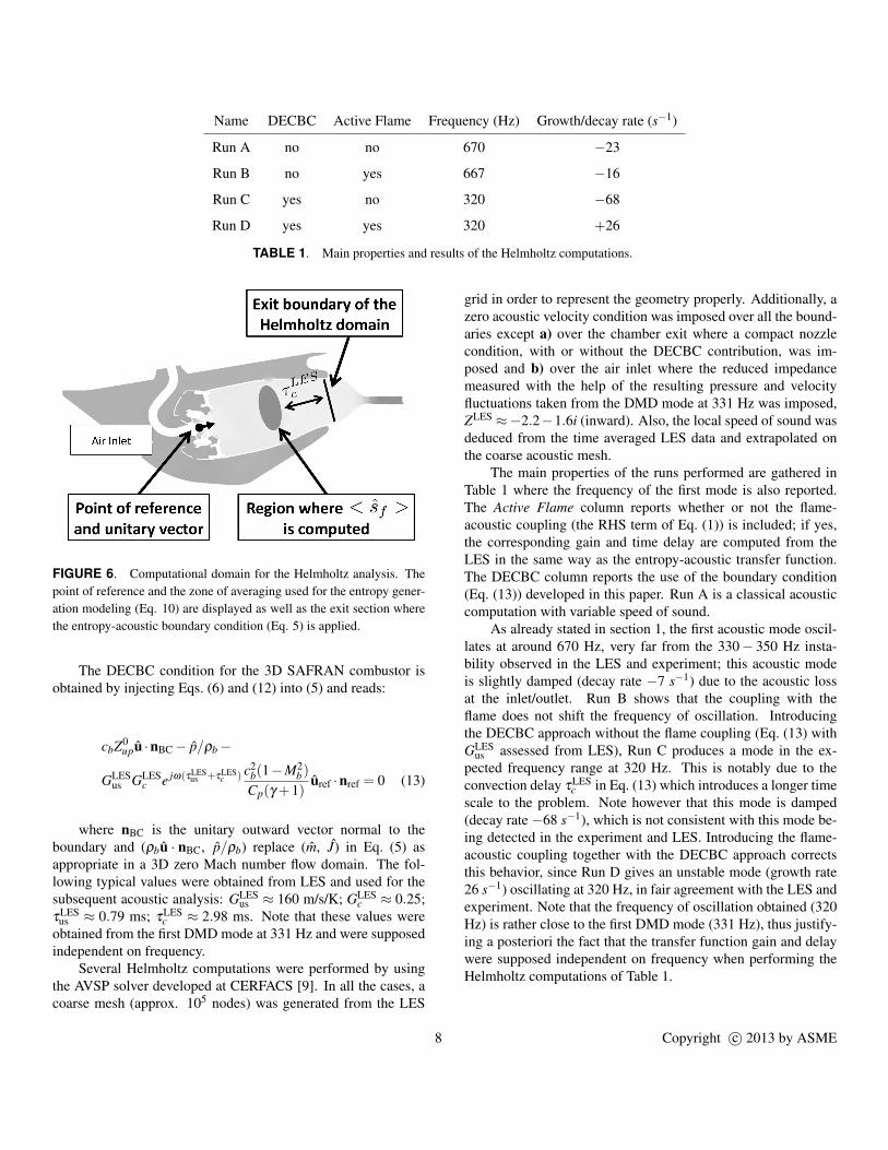
Name DECBC Active Flame Frequency (Hz) Growth/decay rate (s−1)

Run A no no 670 −23

Run B no yes 667 −16

Run C yes no 320 −68

Run D yes yes 320 +26

TABLE 1. Main properties and results of the Helmholtz computations.

FIGURE 6. Computational domain for the Helmholtz analysis. Thepoint of reference and the zone of averaging used for the entropy gener-ation modeling (Eq. 10) are displayed as well as the exit section wherethe entropy-acoustic boundary condition (Eq. 5) is applied.

The DECBC condition for the 3D SAFRAN combustor isobtained by injecting Eqs. (6) and (12) into (5) and reads:

cbZ0upu ·nBC − p/ρb −

GLESus GLES

c e jω(τLESus +τLES

c ) c2b(1−M2

b)

Cp(γ +1)uref ·nref = 0 (13)

where nBC is the unitary outward vector normal to theboundary and (ρbu · nBC, p/ρb) replace (m, J) in Eq. (5) asappropriate in a 3D zero Mach number flow domain. The fol-lowing typical values were obtained from LES and used for thesubsequent acoustic analysis: GLES

us ≈ 160 m/s/K; GLESc ≈ 0.25;

τLESus ≈ 0.79 ms; τLES

c ≈ 2.98 ms. Note that these values wereobtained from the first DMD mode at 331 Hz and were supposedindependent on frequency.

Several Helmholtz computations were performed by usingthe AVSP solver developed at CERFACS [9]. In all the cases, acoarse mesh (approx. 105 nodes) was generated from the LES

grid in order to represent the geometry properly. Additionally, azero acoustic velocity condition was imposed over all the bound-aries except a) over the chamber exit where a compact nozzlecondition, with or without the DECBC contribution, was im-posed and b) over the air inlet where the reduced impedancemeasured with the help of the resulting pressure and velocityfluctuations taken from the DMD mode at 331 Hz was imposed,ZLES ≈−2.2−1.6i (inward). Also, the local speed of sound wasdeduced from the time averaged LES data and extrapolated onthe coarse acoustic mesh.

The main properties of the runs performed are gathered inTable 1 where the frequency of the first mode is also reported.The Active Flame column reports whether or not the flame-acoustic coupling (the RHS term of Eq. (1)) is included; if yes,the corresponding gain and time delay are computed from theLES in the same way as the entropy-acoustic transfer function.The DECBC column reports the use of the boundary condition(Eq. (13)) developed in this paper. Run A is a classical acousticcomputation with variable speed of sound.

As already stated in section 1, the first acoustic mode oscil-lates at around 670 Hz, very far from the 330− 350 Hz insta-bility observed in the LES and experiment; this acoustic modeis slightly damped (decay rate −7 s−1) due to the acoustic lossat the inlet/outlet. Run B shows that the coupling with theflame does not shift the frequency of oscillation. Introducingthe DECBC approach without the flame coupling (Eq. (13) withGLES

us assessed from LES), Run C produces a mode in the ex-pected frequency range at 320 Hz. This is notably due to theconvection delay τLES

c in Eq. (13) which introduces a longer timescale to the problem. Note however that this mode is damped(decay rate −68 s−1), which is not consistent with this mode be-ing detected in the experiment and LES. Introducing the flame-acoustic coupling together with the DECBC approach correctsthis behavior, since Run D gives an unstable mode (growth rate26 s−1) oscillating at 320 Hz, in fair agreement with the LES andexperiment. Note that the frequency of oscillation obtained (320Hz) is rather close to the first DMD mode (331 Hz), thus justify-ing a posteriori the fact that the transfer function gain and delaywere supposed independent on frequency when performing theHelmholtz computations of Table 1.


A limitation of the proposed approach is that theHelmholtz/DECBC solver must be fed by data coming from LESresults. This may appear as a strong limitation since the costof a LES must be paid before the DECBC methodology canbe applied. Still, the Helmholtz/DECBC approach remains use-ful in situations where the same upstream velocity-exit entropytransfer function can be reused for multiple test conditions. An-other potential field of application is the study of annular com-bustors; in this case, one can imagine that a simple one sectorLES (containing only one burner) could be performed to feed aHelmholtz/DECBC computation of the whole annular combustorwith several identical burners, thus avoiding the extremely CPUdemanding LES of the full combustor. This strategy is justifiedif the flames behave independently and was already used for ac-counting for the flame response in annular combustors [20, 21].

4 ConclusionA Delayed Entropy Coupled Boundary Condition was devel-

oped as a means to recover some of the convective effects whenrepresenting a thermo-acoustic system under the zero Mach num-ber formalism. In this view, a simple model was first used inorder to assess the entropy fluctuations at the exit of the combus-tion chamber. This modeling consists of two steps, one for theentropy generation in the flame region, a second one for the con-vection/dissipation of the entropy spots through the combustionchamber. This results in a transfer function which relates a refer-ence acoustic velocity in the burner and entropy at the exit of thechamber and which was assessed by post-processing LES data.The acoustics generated by the convection of the entropy spotsthrough the exit nozzle are then treated by applying a properboundary condition which couples entropy and acoustic quanti-ties. The latter was deduced from the theory of compact nozzlesin the present paper. The computation of a SAFRAN combus-tor which exhibits a low frequency instability demonstrates thepotential of the method.

AcknowledgmentsE. Motheau gratefully acknowledges support from

SNECMA. The authors also thank T. Jaravel and J. Richard(CERFACS) for their technical support for the DMD analysis aswell as Y. Mery (SNECMA) for providing the data. Part of thisstudy has been performed during the Summer Program 2012 ofthe Center for Turbulence Research, Stanford University.

REFERENCES[1] Rayleigh, L., 1878. “The explanation of certain acoustic

phenomena”. Nature, July 18, pp. 319–321.[2] Lieuwen, T., and Yang, V., 2005. “Combustion instabilities

in gas turbine engines. operational experience, fundamental

mechanisms and modeling”. In AIAA Prog. in Astronau-tics and Aeronautics , Vol. 210.

[3] Culick, F. E. C., and Kuentzmann, P., 2006. UnsteadyMotions in Combustion Chambers for Propulsion Systems.NATO Research and Technology Organization.

[4] Hield, P., Brear, M., and Jin, S., 2009. “Thermoacousticlimit cycles in a premixed laboratory combustor with openand choked exits”. Combust. Flame , 156(9), pp. 1683–1697.

[5] Huang, Y., and Yang, V., 2004. “Bifurcation of flame struc-ture in a lean premixed swirl-stabilized combustor: Transi-tion from stable to unstable flame”. Combust. Flame , 136,pp. 383–389.

[6] Schmitt, P., Poinsot, T., Schuermans, B., and Geigle, K. P.,2007. “Large-eddy simulation and experimental study ofheat transfer, nitric oxide emissions and combustion insta-bility in a swirled turbulent high-pressure burner”. J. FluidMech. , 570, pp. 17–46.

[7] Poinsot, T., and Veynante, D., 2005. Theoretical and Nu-merical Combustion. R.T. Edwards, 2nd edition.

[8] Crocco, L., 1952. “Aspects of combustion instability in liq-uid propellant rocket motors. part II.”. J. American RocketSociety , 22, pp. 7–16.

[9] Nicoud, F., Benoit, L., Sensiau, C., and Poinsot, T., 2007.“Acoustic modes in combustors with complex impedancesand multidimensional active flames”. AIAA Journal , 45,pp. 426–441.

[10] Nicoud, F., and Wieczorek, K., 2009. “About the zero machnumber assumption in the calculation of thermoacoustic in-stabilities”. Int. J. Spray and Combustion Dynamic, 1,pp. 67–112.

[11] Marble, F. E., and Candel, S., 1977. “Acoustic distur-bances from gas nonuniformities convected through a noz-zle”. J. Sound Vib. , 55, pp. 225–243.

[12] Leyko, M., Nicoud, F., and Poinsot, T., 2009. “Comparisonof direct and indirect combustion noise mechanisms in amodel combustor”. AIAA Journal , 47(11), pp. 2709–2716.

[13] CERFACS, 2009. AVBP Handbook - http://cerfacs.fr/∼avbp/AVBP V5.X/HANDBOOK. CERFACS.

[14] Colin, O., Ducros, F., Veynante, D., and Poinsot, T., 2000.“A thickened flame model for large eddy simulations ofturbulent premixed combustion”. Phys. Fluids , 12(7),pp. 1843–1863.

[15] Franzelli, B., Riber, E., Sanjose, M., and Poinsot, T.,2010. “A two-step chemical scheme for Large-Eddy Simu-lation of kerosene-air flames”. Combust. Flame , 157(7),pp. 1364–1373.

[16] Poinsot, T., and Lele, S., 1992. “Boundary conditions fordirect simulations of compressible viscous flows”. J. Com-put. Phys. , 101(1), pp. 104–129.

[17] Schmid, P. J., 2010. “Dynamic mode decomposition of nu-


merical and experimental data”. J. Fluid Mech. , 656,pp. 5–28.

[18] Motheau, E., Nicoud, F., and Poinsot, T., 2012. “Usingboundary conditions to account for mean flow effects in azero mach number acoustic solver”. J. Eng. Gas Turb. andPower , 134(11), p. 111502.

[19] Dowling, A. P., 1995. “The calculation of thermoacousticoscillations”. J. Sound Vib. , 180(4), pp. 557–581.

[20] Wolf, P., Staffelbach, G., Gicquel, L. Y., Muller, J.-D., andPoinsot, T., 2012. “Acoustic and large eddy simulationstudies of azimuthal modes in annular combustion cham-bers”. Combust. Flame , 159(11), pp. 3398 – 3413.

[21] Sensiau, C., Nicoud, F., and Poinsot, T., 2009. “A tool tostudy azimuthal and spinning modes in annular combus-tors”. Int. Journal Aeroacoustics, 8(1), pp. 57–68.


draft: analysis and modelling of entropy modes in a realistic aeronautical gas...

Documents